Technical note: Testing the effect of different pumping rates on pore-water sampling for ions, stable isotopes, and gas concentrations in the hyporheic zone

The hyporheic zone (HZ) is of major importance for carbon and nutrient cycling as well as for the ecological health of stream ecosystems, but it is also a hot spot of greenhouse gas production. Biogeochemical observations in this ecotone are complicated by a very high spatial heterogeneity and temporal dynamics. It is especially difficult to monitor changes in gas concentrations over time because this requires pore-water extraction, which may negatively affect the quality of gas analyses through gas losses or other sampling artifacts. In this field study, we wanted to test the effect of different pumping rates on gas measurements and installed Rhizon samplers for repeated pore-water extraction in the HZ of a small stream. Pore-water sampling at different pumping rates was combined with an optical sensor unit for in situ measurements of dissolved oxygen and a depth-resolved temperature monitoring system. While Rhizon samplers were found to be highly suitable for pore-water sampling of dissolved solutes, measured gas concentrations, here CH₄, showed a strong dependency of the pumping rate during sample extraction, and an isotopic shift in gas samples became evident. This was presumably caused by a different behavior of water and gas phase in the pore space. The manufactured oxygen sensor could locate the oxic–anoxic interface with very high precision. This is ecologically important and allows us to distinguish between aerobic and anaerobic processes. Temperature data could not only be used to estimate vertical hyporheic exchange but also depicted sedimentation and erosion processes. Overall, the combined approach was found to be a promising and effective tool to acquire time-resolved data for the quantification of biogeochemical processes in the HZ with high spatial resolution.

1 Introduction

The hyporheic zone (HZ) is the interstitial habitat below streams and rivers, adjacent to and influenced by the stream water above and the groundwater below (Peralta-Maraver et al., 2018). The importance of this zone for stream ecosystems has long been recognized (Boulton et al., 1998) and is emphasized until today (Lewandowski et al., 2019). Ecosystem functions of the HZ include rapid carbon and nutrient recycling (Findlay, 1995; Sophocleous, 2002); physical, chemical, and biological filtration of stream water (Hancock et al., 2005); and flood wave retention (Boulton et al., 1998). The HZ also serves as a habitat for microbiota and macro-zoobenthos (Hendricks, 1993; Robertson and Wood, 2010), provides spawning grounds for fish (Malcolm et al., 2005; Sternecker and Geist, 2010; Smialek et al., 2021), and is important as a juvenile habitat for endangered freshwater mussels (Auerswald and Geist, 2018; Denic and Geist, 2015). On the other hand, as a result of the high microbial activity, greenhouse gas (GHG) production can be substantial in the HZ (Trimmer et al., 2012; Stanley et al., 2016), making many rivers net methane (CH₄), nitrous oxide (N₂O), and carbon dioxide (CO₂) emitters (Romeijn et al., 2019; Saunois et al., 2020).

Therefore, a deep understanding of the processes in the HZ is essential in many disciplines (Krause et al., 2011). High spatiotemporal heterogeneity is making data acquisition for model development and calibration a challenge (Braun et al., 2012). The HZ is a complex system, influenced by many interrelated factors, and more observations are needed to better describe the hydrological, geochemical, and ecological functioning of this dynamic zone.

Well-known approaches to investigating HZ biogeochemistry are direct sediment sampling or pore-water sampling from sediment cores. Water samples can be extracted from cores by centrifugation (Emerson et al., 1980), squeezing (Bender et al., 1987) or pressurization (Jahnke, 1988). However, coring, transportation, and water extraction may disturb the sample and significantly deteriorate sample quality. Sediment sampling also disturbs the sampling site, limits spatial resolution, and can change geochemical gradients through the introduction of bypass flow along boreholes and sampling devices. These issues are critical in the HZ, where geochemical gradients are often steep. Pore-water equilibrium dialysis samplers (peepers), as first described by Hesslein (1976), can be used to obtain pore-water concentration profiles without coring at a high vertical resolution (e.g., Michaelis et al., 2022). A disadvantage is that samples represent an average over the sampling period of (usually) several weeks, making it impossible to observe short-term temporal dynamics typical of the HZ (Boano et al., 2014). Further, both sampling from sediment cores or peepers is not suitable for long-term observations due to perturbation during sampling and the necessity to sample at slightly different positions.

For in situ measurements, microsensors have been developed which can be driven into the sediment to record dissolved O₂ or HS⁻ concentrations, pH, and redox potential with a vertical resolution in the millimeter range (Boetius and Wenzhöfer, 2009). These sensors have been employed at the sea floor (e.g., Vonnahme et al., 2020), but they are not suitable for rivers or streams with high flow velocities or coarse-grained sediments due to their high fragility. In addition, sensors and additional instrumentation for precise handling are very expensive.

Several methods have been developed and applied for direct pore-water extraction from the HZ. The USGS MINIPOINT sampler consists of several steel drive points with different lengths for the extraction of pore water from several depths (Duff et al., 1998). In a similar way, depth-resolved hyporheic pore-water sampling has been realized with multi-level piezometers, a set of tubes with different types of screens at the tips (Rivett et al., 2008; Schaper et al., 2018; Krause et al., 2012), or with fixed PVC or silicon tubes attached to syringes (Geist and Auerswald, 2007; Casas‐Mulet et al., 2021). Rhizon samplers (microfilter tubes), typically applied for soil moisture measurements in the unsaturated zone, have also occasionally been used for pore-water extraction: Rhizon samplers were used for pore-water extraction from sediment cores by Shotbolt (2010), in combination with an in situ chamber in the Wadden sea by Seeberg‐Elverfeldt et al. (2005), and to sample pore water from lake sediment microcosms by Song et al. (2003). From each of these systems, samples can either be extracted with syringes or peristaltic pumps (Seeberg‐Elverfeldt et al., 2005; Knapp et al., 2017).

However, these methods have rarely been used for gas analyses in hyporheic pore water. A vacuum can lead to outgassing, and, therefore, when pulling out the samples, gas contents may be affected. Suitable pumping rates for pore-water extraction have been evaluated from chloride gradients, and rates < 4.0 mL min⁻¹ were found to be acceptable (Duff et al., 1998). But the effect of pumping rates on gas concentrations has never been tested. Especially in fine-grained bed substrates, where the pressure in the extraction system to maintain these flow rates has to be much lower than ambient pressure, degassing effects are no longer negligible. Gas concentrations will reflect the low pressure in the extraction system, which is very hard to measure. In this study, we wanted to test this hypothesis and installed a monitoring station at a site with fine-grained deposits close to the riverbank where high CH₄ concentrations were to be expected. Fifteen Rhizon samplers were installed with a 3 cm vertical distance for repeated pore-water sampling. Three different pumping rates for pore-water sampling were tested and the results were compared to geochemical profiles observed with a peeper that was installed very close to the Rhizon samplers.

The sampling station was amended with a custom-coated fiber-optic oxygen sensor unit based on the description of Brandt et al. (2017) for a precise allocation of the oxic–anoxic interface. Air contamination during sample extraction from sediment cores, peeper chambers, or other types of in situ samplers is likely and problematic for studying anoxic processes. An in situ sensor was therefore essential for the assessment of CH₄ in the HZ. As a third component, temperature monitoring at 14 different depths was used for an estimation of hyporheic exchange. Flux rates were calculated with analytical models introduced by Hatch et al. (2006) and Keery et al. (2007) using the software package VFLUX (Gordon et al., 2012). The temperature data were also needed for evaluating raw data of the O₂ sensor.

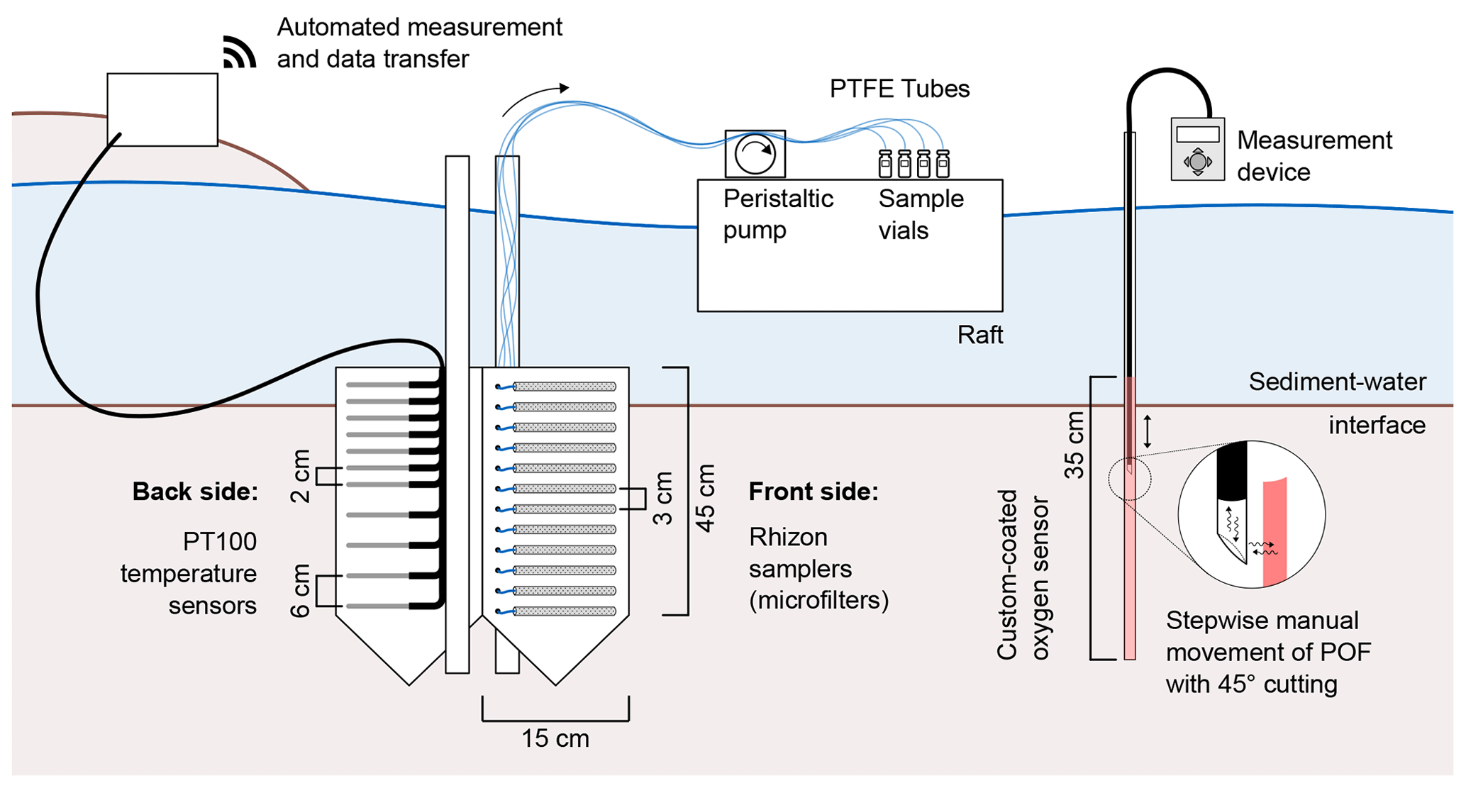
Figure 1 Design of the monitoring station at the Moosach River, Freising, Germany. For reasons of clarity, the schematic figure does not show all sensors.

2 Methods

2.1 Study site and station design

The study was conducted at the Moosach River in southern Germany, close to the city of Freising. The river has a catchment area of 175 km² and is characterized by a low gradient and a high fraction of fines in the streambed (Auerswald and Geist, 2018). The Moosach River is characterized by very uniform flow conditions due to regulations of the water level by weirs. This lack of dynamics is also considered one of the reasons for its stable streambed material with high rates of fine sediment deposition (Auerswald and Geist, 2018). The area where the sampling site was situated lies upstream of a weir that keeps the headwater level nearly constant at almost all discharge conditions. The sampling station was installed on the right bank of the river in a low-flow zone with fine, organic-rich deposits. The grain size distribution of the deposits consisted of 3 % gravel, 27 % sand, and 70 % silt with a porosity of 81.5 % (Sect. S1 in the Supplement). The organic matter content was 21 %. High CH₄ production was expected due to the high content of fines and organic matter (Bodmer et al., 2020). Water depth at the site was approximately 0.6 m.

The monitoring station was installed on 15 March 2021. For installation, a protective casing was manually pushed into the streambed, the interior of the casing was cleared of sediment to allow the sampler to be inserted without damaging the filter tubes or temperature sensors, and finally the protective casing was removed and the sampler left to settle in. After installation, we observed heavy sedimentation and during the summer months, mainly between July and September, major macrophyte growth. The first sampling campaign was done 2 weeks after installation, when disturbances caused by the installation were wearing off. Ten more sampling campaigns were performed in 2021 and three in 2022 (Sect. S1, Table S1 in the Supplement).

The sampling station comprised 15 Rhizon samplers for depth-resolved pore-water sampling (Sect. 2.2), a self-manufactured oxygen sensor (Sect. 2.5), and 14 temperature sensors (Sect. 2.6). Figure 1 shows all components of the sampling station. Rhizon samplers and temperature sensors were fixed horizontally on opposite sides of a Plexiglas (PMMA) panel. The panel was inserted longitudinally to the flow direction in order to keep disturbances to river flow and horizontal hyporheic fluxes to a minimum. Rhizon samplers faced towards the main channel, while temperature sensors faced towards the riverbank. A swimming raft allowed access to the tubes connected to the Rhizon samplers to guarantee sampling without sediment disruption. Temperature sensors were connected to data loggers installed on land next to the river. A fiber-optic measurement system for O₂ concentration was placed right next to the sampling station. With the custom-made optical sensor, an oxygen meter, and an optical fiber, O₂ saturation could be measured with a depth resolution of 1 cm.

Clogging of the Rhizon samplers with a pore size of 0.12–0.18 µm occurred only once shortly after initial installation at three samplers above the sediment–water interface due to biofilm growth. After replacing the top three samplers, this problem did not reoccur. No problems with clogging occurred at the samplers within the sediment. To avoid potential clogging, 2 mL of pore water still in the sampling tubes after each sampling campaign was backwashed.

2.1.1 Pore-water sampling with Rhizon samplers

Our sampling station was equipped with 15 Rhizon samplers with a pore diameter of 0.12–0.18 µm and a filter length of 5 cm (Rhizosphere, Wageningen, The Netherlands). The samplers were fixed horizontally with 3 cm distances. Polytetrafluorethylene (PTFE) tubes with a 1.32 mm inner diameter (Cole-Parmer, St. Neots, UK) were connected to the samplers to lead pore-water samples to the water surface. The material was chosen for its low gas permeability.

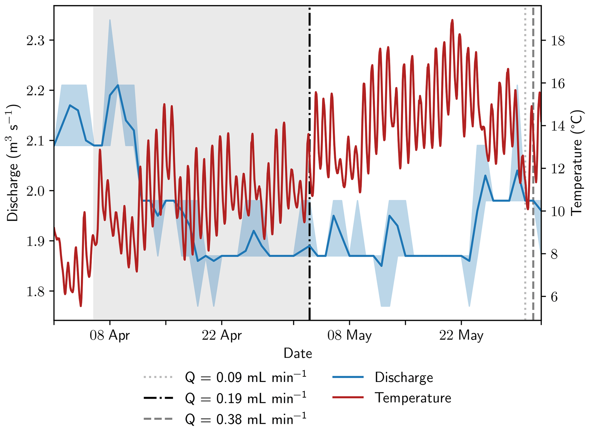
Figure 2 Discharge and stream temperatures during the sampling period. Discharge data from a monitoring station approximately 5 km downstream was retrieved from the Bavarian State Office of the Environment (2023). The span between minimum and maximum discharge is shaded in light blue; average stream discharge is shown as a blue line. The equilibration period of the peeper is highlighted with gray background color. Vertical lines show sampling dates at the monitoring station and are coded to the sampling rates.

Samples were extracted simultaneously from all 15 Rhizon samplers with two ISM 1089 Ismatec Ecoline peristaltic pumps (VWR International, Darmstadt, Germany) with eight cassettes each and gastight Viton peristaltic tubing with an inner diameter of 0.51 mm (Cole-Parmer GmbH, Wertheim, Germany). Three pumping rates were tested in 2022: 0.09 mL min⁻¹ on 30 May, 0.19 mL min⁻¹ on 3 May, and 0.38 mL min⁻¹ on 31 May. Prior to sampling, 4 mL of pore water was taken for pre-rinsing to exchange at least the tube volume of 3.8 mL without increasing the sampling volume too much. Stream temperature conditions were similar on all sampling days; discharge was 0.09 m³ s⁻¹ (4.8 %) higher at the end of May compared to the beginning of the month (Fig. 2). It should be mentioned that the application of a vacuum results in degassing. As the actual pressure conditions cannot be measured, this change in the sample cannot be fully quantified. Calculations indicate that the effect is more pronounced at higher gas concentrations and affects not only the gases but also the pH value and the concentration of bicarbonate.

Samples for stable water isotopes and anion and cation analyses were collected in 1.5 mL glass vials without headspace. For gas analyses, 10 mL glass vials were crimped gastight with butyl rubber stoppers and flushed with synthetic air (O₂, N₂). Right before sampling, 3 mL synthetic air was removed from the enclosed vials. Rubber stoppers were then pierced with needles connected to the peristaltic tubing and 3 mL of sample were pumped directly into the vial, providing a completely gastight, pressure-compensated sampling technique. Samples for gas analyses were fixated with 20 µL 10 M NaOH (Carl Roth, Karlsruhe, Germany). For sulfide measurements, 15 mL Falcon tubes were prepared with 1 mL 1 M zinc acetate (Carl Roth, Karlsruhe, Germany). A sample of 4 mL was injected slowly from below to allow precipitation of ZnS before air contact. All samples were transported in a cooler and stored refrigerated prior to analysis.

2.1.2 Pore-water sampling with a peeper

As a second pore-water sampling method, a pore-water dialysis sampler (peeper) was used. The body of the peeper was equipped with two columns of 38 chambers, each being filled with deionized water and covered with a semipermeable membrane (pore diameter 0.2 µm) (Pall Corporation, Dreieich, Germany). Over a period of 1 month, between 3 April and 3 May, an equilibrium between the water in the chambers and the surrounding pore water was obtained. Immediately after removing the peeper from the sediment, the water from the chambers was extracted with syringes and injected into vials. Due to the low amount of available sample volume (on average 3 mL per chamber), pore-water analysis was restricted to anion, cation, and CH₄ concentrations along with the stable carbon isotope ratio (δ¹³C) of CH₄. Samples for anion and cation analysis were stored in 1.5 mL glass vials. Samples were fixated with 10 µL 0.5 M NaOH (anions) and 10 µL 1 M HCl (cations) to cope with long analysis times due to the large number of samples. Vial preparation for gas analyses, including fixation, flushing, and sealing, was similar to the sampling method described in Sect. 2.1.1. During sample injection, two syringes were used: one for the sample and one to allow pressure exchange. Both needles were removed directly after sampling.

Dissolved O₂ concentrations were measured in the field immediately after retrieval of the peeper from the sediment and its cleaning with deionized water. A Clark-type microsensor (Unisense, Aarhus, Denmark) was pierced through the membrane for the measurements (Revsbech, 1989). A time constraint on this technique is contamination with atmospheric O₂, which can diffuse quickly through the membrane under air contact. Thus, O₂ measurements had to be conducted as rapidly as possible and only selected chambers were tested to avoid artifacts.

2.2 Analytical methods for pore-water analysis

Anion and cation concentrations were measured with a system of two ICS-1100 ion chromatographs (Thermo Fisher Scientific) equipped with Dionex IonPacTM AS9-HC and CS12A columns, respectively. All results represent an average of triplicate measurements and were evaluated based on seven calibration standards (Merck, Darmstadt, Germany) reaching an analytical uncertainty of <10 %. Detection limits were 0.039 mmol L⁻¹ for Ca²⁺, 0.032 mmol L⁻¹ for Mg²⁺, 0.020 mmol L⁻¹ for Cl⁻, 0.012 mmol L⁻¹ for NO${}_{\mathrm{3}}^{-}$, 0.007 mmol L⁻¹ for NO${}_{\mathrm{2}}^{-}$, and 0.008 mmol L⁻¹ for SO${}_{\mathrm{4}}^{\mathrm{2}-}$.

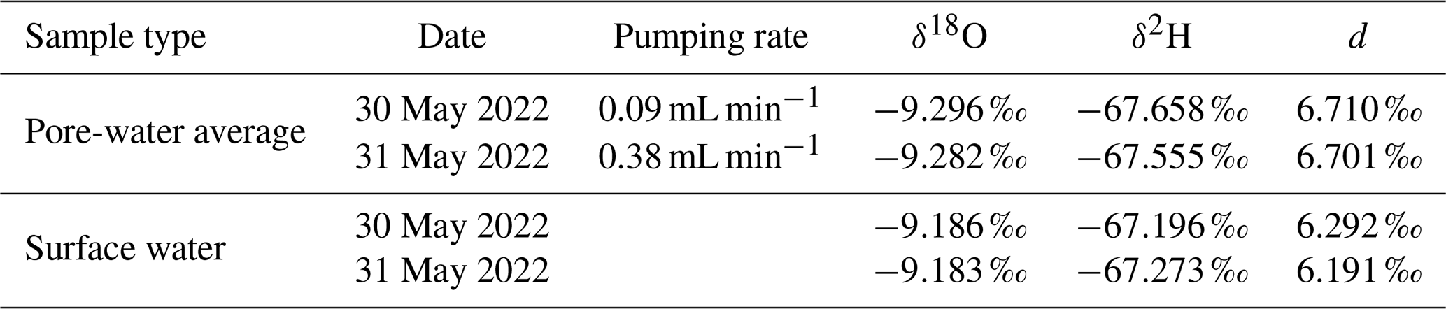
Stable water isotopes were measured in the same vials which had been used for cation analysis or in completely filled 1.5 mL glass vials that had been sampled separately. Only samples without acid or a base addition for fixation could be used. Fixation was necessary for peeper samples and Rhizon samples for the median pumping rate of 0.19 mL min⁻¹ (same sampling date) due to the high number of samples and long expected analysis times. Samples were analyzed with the IWA-45EP isotopic water analyzer (Los Gatos Research, San Jose, USA) calibrated with three standards (USGS Reston Stable Isotope Laboratory, Reston, USA) with an analytical error of <0.1 ‰ for δ¹⁸O and <1 ‰ for δ²H. Results are expressed in the δ notation relative to the V-SMOW standard. Deuterium excess was calculated as $d={\mathit{\delta }}^{\mathrm{2}}\mathrm{H}-\mathrm{8}\cdot {\mathit{\delta }}^{\mathrm{18}}\mathrm{O}$ (Dansgaard, 1964).

Methane concentrations were measured according to a procedure introduced by the US Environmental Protection Agency (EPA, 2001) adapted for small sample volumes. Before analysis, vials were left for equilibration at 30 ^∘C for at least 2 h. Headspace CH₄ concentrations were measured with a Trace 1300 gas chromatograph (GC) (Thermo Fisher Scientific, Dreieich, Germany) with a TG-5MS column and flame-ionization detector (FID), calibrated with three concentration standards (Rießner Gase, Lichtenfels, Germany). Samples were measured in triplicates of 250 µL manual headspace gas injection. Calculations of total concentrations before equilibration with the headspace were based on Henry's law as previously described (Kampbell and Vandegrift, 1998; EPA, 2001).

The vials for CH₄ concentration measurements were also used for isotopic analyses with a G2201-i gas analyzer (Picarro, Santa Clara, USA) for ${}^{\mathrm{12}}\mathrm{C}/{}^{\mathrm{13}}\mathrm{C}$ ratios in CH₄ with an analytical uncertainty of <0.16 ‰. Headspace vials were directly connected to the Small Sample Introduction Module (SSIM) with needles. Dilution of the samples with synthetic air and re-pressurization of the glass vials was necessary for repeated measurements due to the small sample and headspace volume. Reliable results could not be obtained at headspace CH₄ concentrations of <30 ppm (Michaelis et al., 2022). Results are represented in the δ notation relative to the V-PDB standard.

Sulfide samples were reactivated in the laboratory by adding 50 µL 49 % H₂SO₄ to dissolve the ZnS precipitate directly before analysis with the 1.14779.001 Spectroquant sulfide test for the Spectroquant Prove 100 photometer (Merck, Darmstadt, Germany). Sulfide concentrations were found to be below the detection limit of 0.02 mg L⁻¹ during several sampling campaigns and were therefore excluded from subsequent sampling and analyses. This may be indicative of very low sulfide concentrations in the HZ, but an issue with sampling or analytical methods cannot be ruled out.

2.3 Statistical analyses

CH₄ concentration, δ¹³C-CH₄, δ¹⁸O-H₂O, δ²H-H₂O, Ca²⁺, Mg²⁺, and Cl⁻ concentration data from peeper and Rhizon measurements at different pumping rates were tested for statistically significant differences. First, data sets were checked for normal distribution with the Shapiro–Wilk test and a visual inspection of box plots. Levene's test was used for assessing the homogeneity of variance. Since the requirements for t tests and the one-directional ANOVA test (normal distribution of all data sets and, for ANOVA, homogeneity of variances) were not met for all data sets, nonparametric tests were chosen. The Mann–Whitney U test was applied for pairwise comparisons and the Kruskal–Wallis H test for assessing differences in more than two data sets, comparing all sampling techniques for each parameter. Independent t tests were used for pairwise comparisons where both data sets were normally distributed. All assessments were implemented in Python (version 3.8.3) using the scipy.stats package (version 1.5.1).

2.4 Dissolved oxygen profiling

Measuring O₂ concentrations in extracted samples had two major disadvantages: sample contamination with atmospheric O₂ during extraction could not be securely excluded and the vertical resolution of 3 cm between the Rhizon samplers was too low to depict the steep O₂ gradient. Therefore, a system for in situ oxygen profiling was constructed and installed.

Following the example of Brandt et al. (2017), an optode for optical O₂ measurements was manufactured by coating a Plexiglas tube with an oxygen-sensitive dye. To produce the sensing element, a sensor cocktail was prepared by dissolving 20 mg of platinum tetrakis(pentafluorophenyl)porphyrin (PtTFPP) (Porphyrin Systems, Lübeck, Germany) and 2 g polystyrene in 10 mL toluene. The sensor cocktail was filled into a glass tube with a punched Viton septum (diameter 4.5 mm) at the lower end where the PMMA tube with an outer diameter of 5 mm (inner diameter of 3 mm) fits tightly. The PMMA tube was then pulled through the sensor solution with a stepper motor at 0.25 cm s⁻¹ and left to dry for at least 12 h yielding a thin oxygen-sensitive coating on the outside of the tube. Measurements were performed with the Fibox 4 trace oxygen meter (PreSens, Regensburg, Germany) connected to a polymeric optical fiber (POF) with an outer diameter of 2.7 mm. The tip of the POF was equipped with a 45^∘ cutting to allow signal transfer orthogonal to the fiber (see Fig. 1).

In contrast to the work of Brandt et al. (2017), the sensor was not connected to an automated motor unit for data recording due to the low stability of the long Plexiglas tube (>75 cm above the sediment–water interface at a water depth of 60 cm) and the risk of water-level changes at high flow. Instead, measurements were performed manually by pulling up the POF in 1 cm steps as marked on the cable. At each depth, at least three measurements were done at a rate of 1 Hz. For each depth, mean and standard deviation of repeated measurements were calculated.

For calibration, distilled water with seven different O₂ concentrations was prepared by stripping with N₂ or He gas for different amounts of time. Each sensor was installed in a flow-through cell which was flushed with the deoxygenated water. Dissolved O₂ concentration in the flow-through cell was in parallel measured with a microsensor (Unisense, Aarhus, Denmark). For temperature control, the flow-through cell was placed in a column connected to a WCR-P22 thermo-controlled water bath (Witeg, Wertheim, Germany). Calibration was conducted at 20 ^∘C. For each sensor, temperature dependence at 0 % and 100 % air saturation (a. s.) was evaluated with five and four temperatures between 5 and 30 ^∘C, respectively. Details on calibration results and the calculation of dissolved O₂ concentrations from measured phase angles can be found in Sect. S3.

2.5 Vertical hyporheic exchange estimation using temperature measurements

Temperature was measured in 14 different depths to trace hyporheic exchange fluxes at the sampling site. The four-wire PT100 sensors (Omega Engineering, Norwalk, USA) with an accuracy of ±0.03 ^∘C were calibrated in a WCR-P22 water bath (Witeg, Wertheim, Germany) with an accuracy of ±0.1 ^∘C at seven different temperatures between 0 and 30 ^∘C before installation in the field. During calibration, sensor recordings were compared to the average temperature considering all sensors yielding a constant correction factor for each sensor.

On site, the sensors were installed with a 2 cm depth resolution for the first 15 and a 6 cm resolution below. Another sensor was placed approximately 20 cm below the water surface in the water column. The sensors were fixed on the back side (facing the riverbank) of the panel holding the Rhizon samplers. The 14 sensors were connected to four PT104A loggers (Omega Engineering, Deckenpfronn, Germany) and a Raspberry Pi-based control unit for automated data acquisition every 5 min.

Due to the long installation time, four out of 14 sensors stopped functioning properly, two additional sensors were excluded from analysis due to data gaps of >24 h. Data processing included the removal of outliers < 0 or >30 ^∘C, interpolation over data gaps < 24 h, and resampling to equally spaced 5 min intervals.

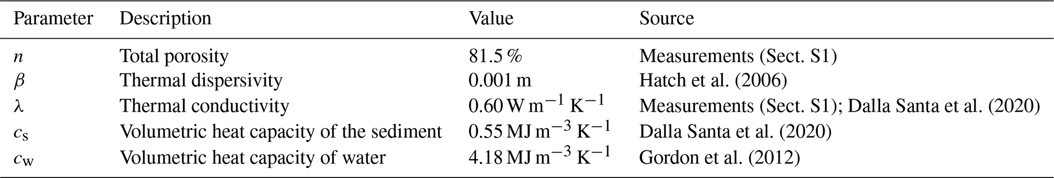
Vertical hyporheic exchange rates were estimated using the software package VFLUX (Gordon et al., 2012). The software implements analytical solutions (Hatch et al., 2006; Keery et al., 2007) to the one-dimensional heat transfer equation for steady fluid flow through a homogeneous porous medium (Stallman, 1965). These solutions use amplitude and phase change in the sinusoidal diurnal signal of a pair of two temperature sensors in different depths for the calculation of the advective flow component. VFLUX first obtains the diurnal oscillation signal by filtering the data using dynamic harmonic regression (DHR) (Young et al., 1999). Then, differences in amplitude and phase are extracted for each periodic cycle. The software calculates vertical flux rates for each specified sensor pair in meters per second based on both amplitude and phase change for each of the methods described by Hatch et al. (2006) and Keery et al. (2007). Sediment-specific input parameters for the calculations are summarized in Table 1.

Hatch et al. (2006)Dalla Santa et al. (2020)Dalla Santa et al. (2020)Gordon et al. (2012)

Table 1 Parameters for vertical hyporheic exchange estimation using the software package VFLUX.

3 Results

3.1 Comparison of pore-water sampling techniques

Geochemical profiles measured in pore-water samples from peeper and Rhizon samplers showed high agreement, especially for stable water isotopes and ions. Figure 3 shows depth profiles measured with a peeper and the Rhizon samplers at three different pumping rates. Rhizon sampling at different pumping rates was conducted in May. NO${}_{\mathrm{3}}^{-}$ and SO${}_{\mathrm{4}}^{\mathrm{2}-}$ concentrations were very similar for all profiles showing steep gradients in close proximity to the sediment–water interface. The low number of samples above the detection limit, together with the steep geochemical gradients, was not sufficient for statistical evaluation. Ca²⁺, Mg²⁺, and Cl⁻ concentrations were on average 5–7 % lower in the peeper data compared to Rhizon samples, but different pumping rates did not have an effect on average concentrations (Sect. S4, Fig. S6).

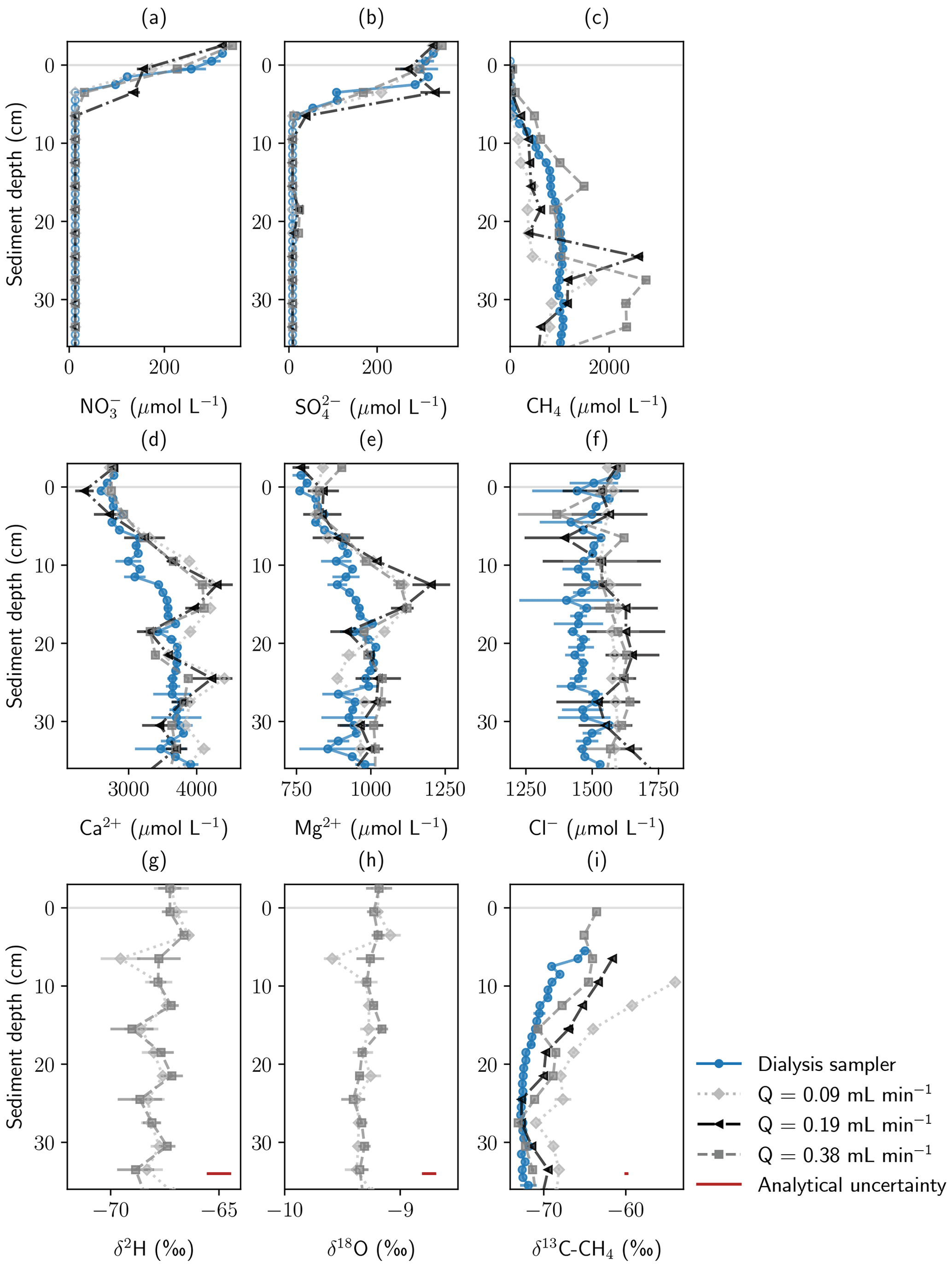
Figure 3 Concentration and stable isotope profiles measured with a pore-water dialysis sampler and Rhizon samplers from the monitoring station at three different pumping rates. All samples were extracted in May 2022. Panels show (a) NO${}_{\mathrm{3}}^{-}$, (b) SO${}_{\mathrm{4}}^{\mathrm{2}-}$, (c) CH₄, (d) Ca²⁺, (e) Mg²⁺, and (f) Cl⁻ concentrations; (g, h) stable water isotopes; and (i) stable carbon isotopes in CH₄. Error bars show standard deviation of repeated measurements. In addition, analytical uncertainty of the measurement devices is shown for isotope data.

Table 2 Stable water isotopes (δ²H and δ¹⁸O) and deuterium excess d in pore water and surface water.

Average CH₄ concentrations in Rhizon samples deviated by −30 % (lowest pumping rate) to +100 % (highest pumping rate) from peeper samples. While the CH₄ concentration profiles recorded with the peeper showed a smooth gradient, profiles from Rhizon measurements showed large concentration differences in consecutive depths. Average measured concentrations were significantly different not only between peeper and Rhizon samples but also for different pumping rates (Fig. S5).

To analyze if isotope fractionation processes influence the measurements of dissolved solutes and gases, stable water isotopes (δ¹⁸O and δ²H) were measured in water samples and stable carbon isotopes (δ¹³C) in methane. Water isotopes were only measured at the highest and lowest pumping rate. Results were found to be similar with no significant differences based on the t test (Sect. S4). Table 2 shows water isotopes from pore-water samples and surface water samples. Deuterium excess in the sediment was 0.5 ‰ higher in pore water compared to surface water samples. This is below the analytical precision for δ²H measurements of 1 ‰.

With an average of −71.2 ‰ CH₄ had a significantly lighter isotopic composition in peeper samples compared to samples extracted with Rhizon samplers (averages between −65.9 ‰ and −69.2 ‰). The stable carbon isotopic composition of CH₄ was with −65.9 ‰ the heaviest at the lowest pumping rate. Homogeneity of variances was neither given in CH₄ concentration nor stable isotope data. Standard deviation of CH₄ concentrations increased with increasing pumping rate (420 µmol L⁻¹ at the lowest pumping rate, 678 µmol L⁻¹ at the medium pumping rate, and 1119 µmol L⁻¹ at the highest pumping rate) but was more similar for isotopic data. When comparing all four data sets with the Kruskal–Wallis H test, differences were significant for both CH₄ concentrations (p=0.01) and stable isotopes (p=0.0003).

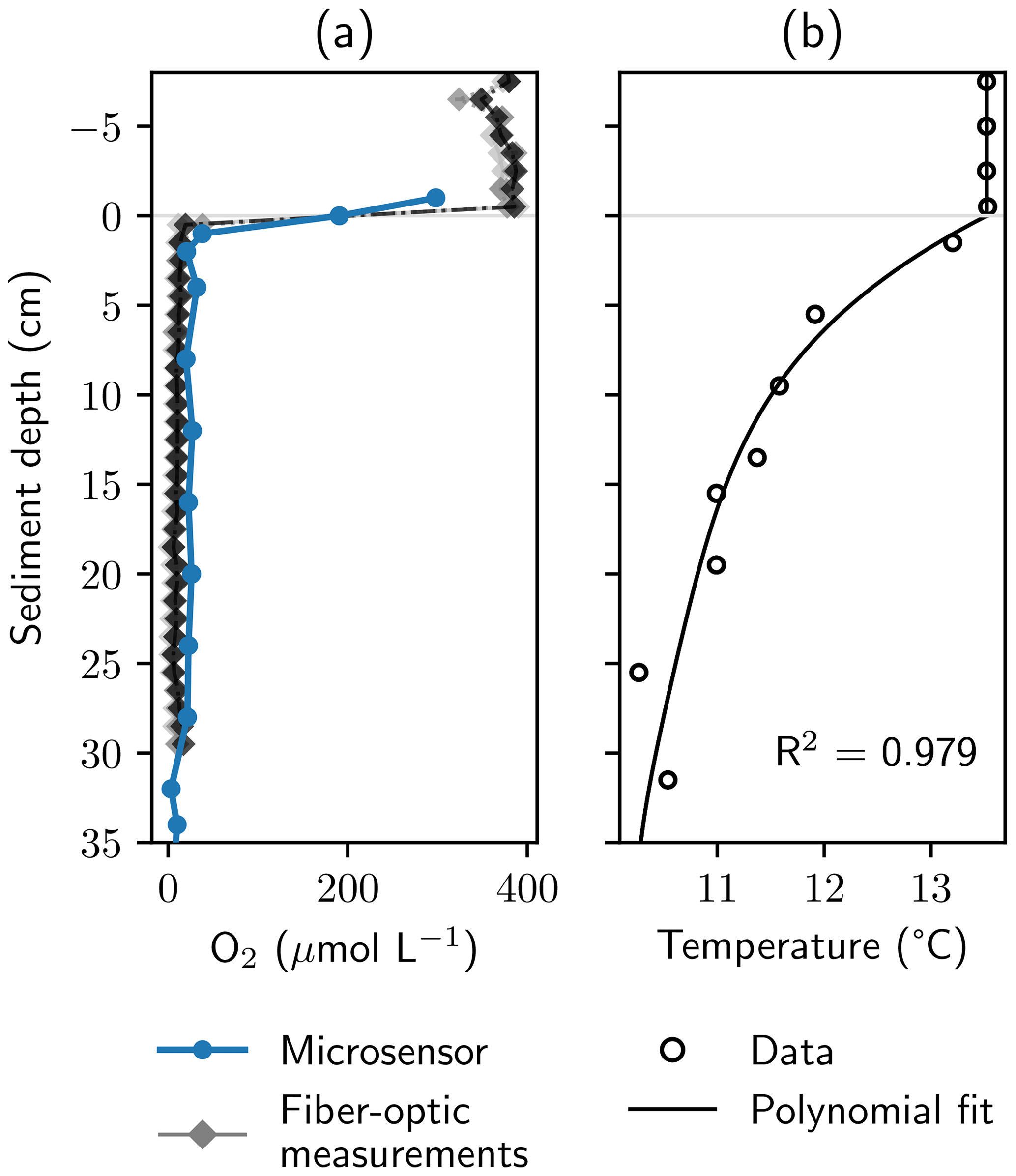
Figure 4 Oxygen and temperature gradients at the study site. Panel (a) shows dissolved O₂ profiles measured with a microsensor in the chambers of a peeper and with a manufactured in situ fiber-optic sensor. Saturated values measured with the fiber-optic system were normalized to avoid unrealistically high values. Panel (b) shows temperature measurements and a fourth-order polynomial fit, which was used to calculate O₂ concentrations from measured phase angles.

In addition, the hyporheic geochemistry of the study site was described in detail with 11 sampling campaigns between April and September 2021 (Sect. S2). Geochemical gradients were found to be very steep, with oxygen reduction and denitrification zones in close proximity or even partly overlapping. A substantial amount of CH₄ was produced in the deep anoxic layers of the HZ. Ion and gas concentrations were stable over time with only gradual changes between spring and summer. The most pronounced changes were sedimentation events which moved the location of the sediment–water interface upwards. The anoxic, reduced conditions in deeper layers stayed unchanged throughout the sampling period in 2021. CH₄ concentration profiles measured with a peeper in September 2021 and in May 2022 showed almost exactly the same gradients.

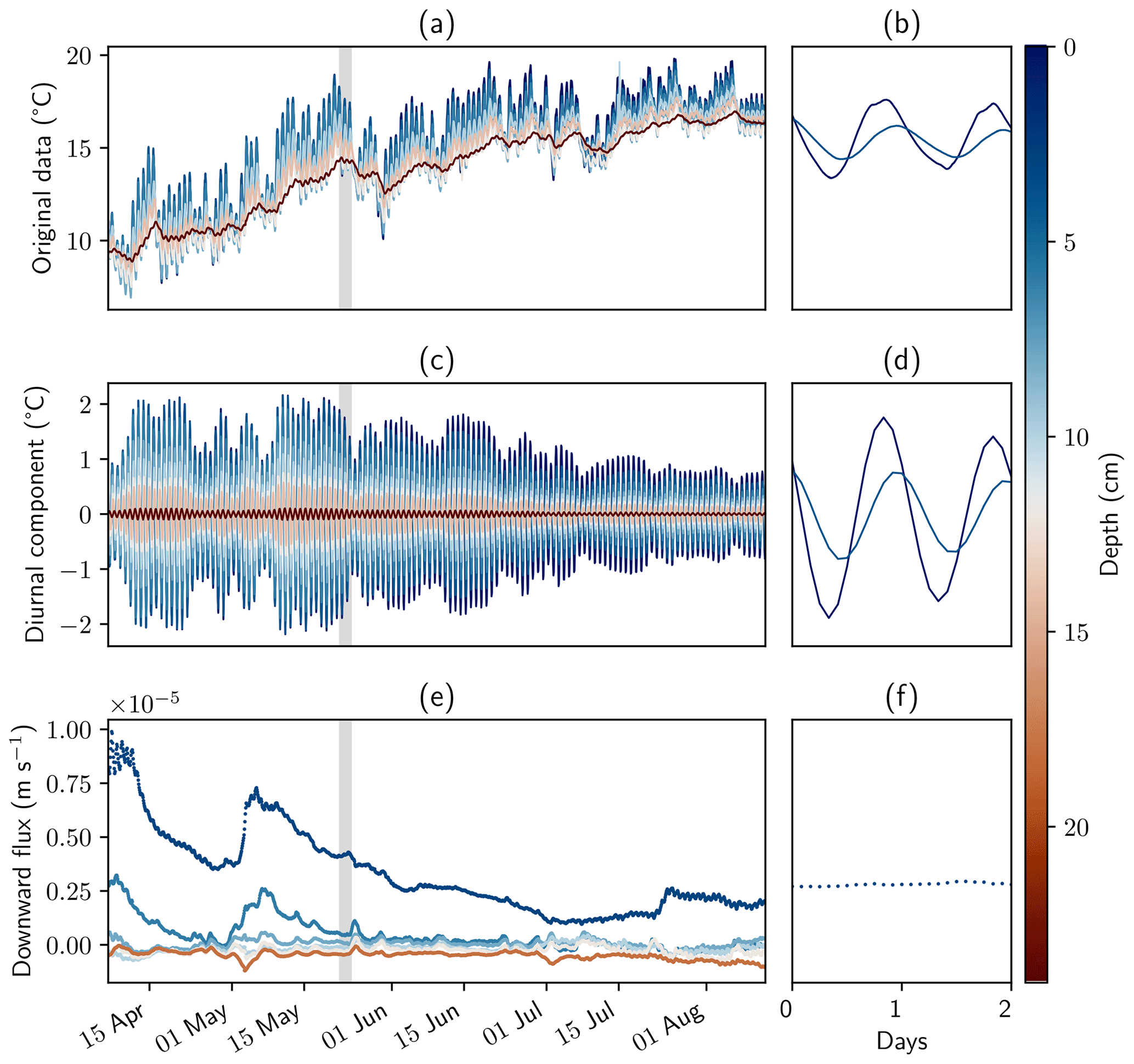
Figure 5 Temperature measurements, filtered data, and calculated fluxes. Panels (a), (c), and (e) show the complete measurement period and all sensors. Panels (b), (d), and (f) show sensors in the surface water and at 10 cm depth for a time window of 2 d. Panels (a) and (b) show original data. Filtered data and fluxes were calculated with the software package VFLUX and the amplitude method described by Hatch et al. (2006) using the parameters from Table 1.

3.2 Locating the oxic–anoxic interface

The fiber-optic sensor unit based on the description of Brandt et al. (2017) was tested against a microsensor in the chambers of the peeper (Fig. 4). The fiber-optic system was able to locate the oxic–anoxic interface precisely. All three repeated measurements showed good agreement at a high resolution of 1 cm. However, the lowest O₂ concentration (20 µmol L⁻¹) measured with the microsensor was higher than dissolved O₂ concentrations observed with the fiber-optic system below the oxic–anoxic interface. In O₂ saturated conditions, absolute values for calculated O₂ concentrations from the fiber-optic system showed high variance. Due to the flat shape of the calibration model in near-saturated conditions (see Sect. S3, Fig. S4), signal noise led to larger errors than in the anoxic zone. Oversaturated values were normalized to avoid unrealistically high values (Eq. S4).

3.3 Assessing vertical hyporheic exchange

Temperature data were continuously recorded between April and August 2022. Pronounced amplitude dampening and time lag of the diurnal signal could be extracted with DHR and subsequently used for flux calculations (Fig. 5). Six sensors had to be excluded from the data set due to low data quality or larger data gaps, leaving a total of eight sensors for the evaluation. Neighboring sensors were not chosen as pairs for sensor flux calculation; instead every other sensor formed a pair, for example sensors 1 and 3, sensors 2 and 4, and sensors 3 and 5. Here, results based on the amplitude method described by Hatch et al. (2006) with the parameters from Table 1 are shown. Fluxes simulated with the phase method and with analytical solutions derived by Keery et al. (2007) are discussed in Sect. S5.

Flux rates calculated with the upper three sensors showed peaks of a downward flux of up to $\mathrm{1}\times {\mathrm{10}}^{-\mathrm{5}}$ m s⁻¹ (85 cm d⁻¹) in April and May 2022. Flux rates calculated between the lower five sensors showed mainly upward-directed flow. Average flux rates at 10, 12, and 18 cm depth were $-\mathrm{1.6}\times {\mathrm{10}}^{-\mathrm{7}}$ m s⁻¹ (−1.4 cm d⁻¹), $-\mathrm{2.6}\times {\mathrm{10}}^{-\mathrm{7}}$ m s⁻¹ (−2.2 cm d⁻¹), and $-\mathrm{4.9}\times {\mathrm{10}}^{-\mathrm{7}}$ m s⁻¹ (−4.2 cm d⁻¹), respectively. This is shown in detail in Sect. S5, Fig. S8, where fluxes calculated for 3 and 6 cm depth were excluded from the plot. Based on these values, mean water transit times in the 40 cm stretch from the bottom to the top of the geochemical profiles would be between 9 to 29 d.

4 Discussion

Our results showed an excellent agreement for ion concentration and stable water isotope measurements in pore-water samples for the two different methods used and equally good agreement for different pumping rates when using Rhizon samplers and peristaltic pumps. The only exceptions were Cl⁻ concentrations, which were consistently higher at the monitoring station compared to the peeper, and Mg²⁺ at medium and high pumping rates (Fig. S6). This indicates a high suitability of Rhizon samplers for repeated pore-water extraction at one specific site to study temporal dynamics in nutrient cycling. Certainly, Rhizons could also be used to trace the fate of contaminants, as long as the pore diameter of the filter allows the contaminant molecule to pass and the contaminant is fully dissolved in water. For concentration and isotope analyses of dissolved gases, here CH₄, we found a lower agreement between pore-water samples extracted by Rhizons and peepers. Gas concentrations and variance increased with increasing pumping rates when using Rhizon samplers. On average, concentrations were lower compared to dialysis measurements.

Based on the data from 2021, which showed a very stable geochemical system, rapid changes in stream geochemistry between the sampling days at the beginning and end of May 2022 are not expected. The stream temperature was very similar on all sampling days, and river discharge was only 4.8 % higher at the end of the month (Fig. 2). Ebullition occurred sporadically, but no larger, sudden gas releases were observed at the sampling site, neither in 2021 nor during recent field campaigns. Therefore, a rapid change in gas concentrations in the sediment seems to be very unlikely and the observed changes in CH₄ concentrations and stable isotopic composition in CH₄ are most likely caused by the changes in pumping rate and not by varying hydrological or geochemical conditions at the sampling site.

Of course, actual changes in gas content and composition between sampling days would explain the measured differences. If these are not triggered by temperature changes or discharge peaks, they could be caused by physical stress or a sudden ebullition event. However, these events seem rather unlikely considering the stagnating geochemistry in 2021 and the rather remote location of the sampling site without public access. The possibility that water is sampled from different parts of the pore space at different pumping rates seems more convincing. Pressure gradients around the samplers will change if the pumping rate is increased.

Another possible explanation for the observed differences in CH₄ concentrations and carbon stable isotopic composition may be differing behaviors of water and gas phases in the interstitial pore space. Rising air bubbles were sporadically observed at the sampling site and entrapped gas was found in sediment cores. During sample extraction, gas was seen to travel upwards through the tubes. These gas bubbles might become trapped in front of the microfilters at low pumping rates because pressure gradients may not be sufficient for the extraction of gas bubbles from the sediment. At higher pumping rates, bubbles seem to get mobilized from a larger distance, potentially further away than liquid pore-water samples. Additionally, a greater vacuum at higher pumping rates may cause increased outgassing and, thus, the creation of additional gas bubbles. Since the tubes were directly connected to the sampling vials, bubbles were not lost, but the gas and water phases were both contained in the sample vial. This could explain the large scatter and high concentration peaks observed at higher pumping rates. Most likely a combination of this effect and the extraction of sample from different parts of the pore space is responsible for the observed differences in gas samples at different pumping rates.

The dependence of CH₄ concentrations on the pumping rate complicates data interpretation because it is unknown from which part of the pore space the gas and water phases were extracted and it is difficult to define a “correct” pumping rate where the gas and water phases are extracted from the same pore space. One also has to consider the trade-off between low pumping rates (low pressure gradient, little degassing) and corresponding sampling times (contact with air, sampling artifacts). Thus, gas measurements in pore-water samples extracted with Rhizon samplers are bound to have significant bias, especially if gas bubbles are present in the system.

Yet, dialysis does not include the gas phase in pore-water measurements at all, and it is questionable if it represents CH₄ distribution accurately. Bubbles cannot enter the chambers of the peeper and therefore, cannot be directly sampled. Contact with the gas bubbles over extended time periods might however increase dissolved CH₄ concentration in the water sample. An effect could be a smoothed concentration gradient with slightly elevated concentrations. In addition, peepers integrate over several weeks while direct pore-water extraction can capture a specific moment in time. Hence, dialysis may not be a better solution for representing the distribution of gaseous and dissolved CH₄ in the sediment.

Other techniques for pore-water extraction such as multi-level piezometers or USGS MINIPOINT were not tested in this study but may have similar advantages and disadvantages to Rhizon samplers. They allow time-resolved measurements and are hypothesized to be better suited for measuring effect and the distribution of gas in sediments than dialysis samplers. But if, as suspected, changes in negative pressure at different pumping rates lead to a different behavior of the gas and water phases in the pore space, this effect is likely to occur whenever samples are directly extracted from the pore space, no matter with which device. Larger pore diameters could increase the suitability for gas sampling, but we would still recommend testing the effect of different pumping rates when working with gas analyses in this type of fine-grained environment.

While sampling had a negligible effect on isotope fractionation for stable water isotopes, measured as proxies for the liquid phase, δ¹³C values of CH₄ showed significant differences in the four measured profiles, showing an isotope fractionation towards heavier carbon isotopes at low pumping rates. At high concentrations (>950 µmol L⁻¹), δ¹³C of CH₄ was found to be similar for sampling with Rhizon samplers and peepers ($-\mathrm{72.0}\pm \mathrm{1.1}$ ‰). Below 950 µmol L⁻¹, a steep nonlinear increase in δ¹³C was observed with decreasing CH₄ concentrations (Fig. 6). The higher stable carbon isotope composition at low concentrations can either be caused by microbial CH₄ degradation (Whiticar and Faber, 1986) or by an isotope fractionation effect during sampling, for example due to diffusion through the tubes or losses at the peristaltic pump. CH₄ escaping through leakages or diffusion would lead to a greater loss of the lighter ¹²CH₄ compared to ¹³CH₄ and an enriched remaining CH₄ pool (Li et al., 2022). This effect is expected to be more pronounced at low concentrations. Effects of microbial degradation would be expected to be in a similar range for peeper and Rhizon-derived profiles; thus δ¹³C values exceeding maximum δ¹³C in peeper samples by up to 10 ‰ imply fractionation during sample extraction.

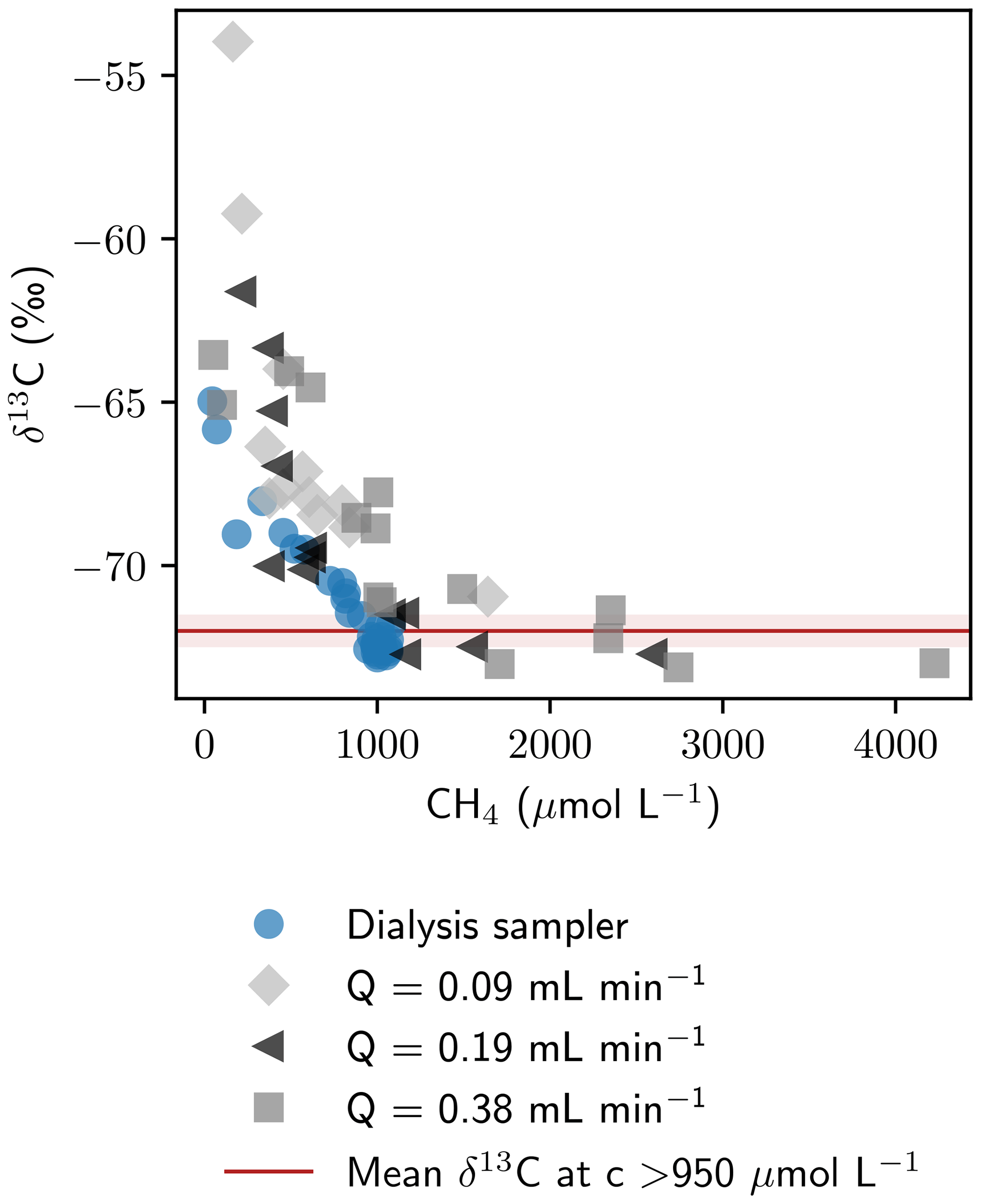
Figure 6 Relation of CH₄ concentrations and isotopic composition. The average ± standard deviation of δ¹³C-CH₄ for all data points with concentrations > 950 µmol L⁻¹ ($-\mathrm{72.0}\pm \mathrm{1.1}$ ‰) is shown in red.

This is true for a very fine-grained sampling site with a high content of organic matter and the occurrence of gas bubbles. In this type of system, the extraction of pore water requires high negative pressures at the interface between sampler and saturated sediment to overcome capillary forces in the sediment. The predominance of gas in the pore space complicates the sampling procedure and data interpretation. In sandy or gravelly riverbeds, lower suction rates are sufficient for pore-water extraction and CH₄ is likely to be present at lower concentrations and, thus, probably completely dissolved in the water phase. In these systems, the problems observed here may not be of relevance. Nevertheless, we find it important to emphasize the potential problems of using Rhizons for gas sampling because this has not been addressed previously in the literature and because Rhizons might be increasingly used in the future, when the interest in the HZ as an important source of GHG rises.

Dissolved O₂ concentrations measured in peeper chambers were elevated compared to in situ measurements and we did not find an affordable way to measure dissolved O₂ concentrations in extracted pore-water samples without contamination with atmospheric air. Considering the steep geochemical gradients, the employed sampling resolution of 3 cm would not have been sufficient to precisely locate the oxic–anoxic interface. For the assessment of CH₄ in a case like this, there is a necessity for in situ measurements. The sensor developed by Brandt et al. (2017) was a low-cost, effective tool and a great addition to the monitoring station. Temperature sensors that were necessary for the evaluation of the O₂ sensor’s raw data could also be used for a continuous monitoring of the sampling site. The data were used to describe the site as an upwelling system, which is important information for the interpretation of geochemical profiles and, in addition, could visualize sedimentation and erosion processes. The measurements could further help to improve geochemical transport models if applied because diffusion coefficients are temperature dependent. However, the installation of the sensors must be done carefully to ensure a long service life. At our field site, several sensors stopped functioning properly, most likely due to problems at soldered joints and connectors or due to humidity and water intrusion.

The combination of pore-water sampling, in situ oxygen profiling, and temperature monitoring allowed a precise characterization of the functioning of the HZ with high spatiotemporal resolution, and the three methods were found to complement each other very well. The combination could, for example, be very useful for studying the effect of floods and droughts on stream ecosystems in terms of nutrient cycling and GHG emission pulses, although additional fastenings may be necessary to ensure stability during floods. So far, to our knowledge, the effect of drying and first flush events on riverine GHG emissions has not been studied, and the described setup would be well suited to tracing the hydrological and geochemical changes in the HZ during such events. The setup could also be used for tracer experiments, since Rhizon samplers cannot only be used for pore-water extraction but also for water injection. This could, for example, benefit the understanding of hyporheic flow patterns or the calculation of mean residence times and carbon or nutrient turnover rates.

5 Conclusions

In this study, we tested three methods for resolving temporal dynamics in HZ geochemistry. Rhizon samplers were found to be suitable for the extraction of water samples and the measurement of dissolved solutes with a high vertical resolution. However, suitability for gas analyses was reduced, as indicated by a dependency of CH₄ concentration on the pumping rate and a fractionation towards heavier isotopes during sampling. This finding might be most pronounced in fine-grained systems with gas inclusions in the sediment, and sampling with Rhizon samplers for gas analyses might be more suitable for rivers with coarser bed substrate and higher hydraulic conductivity, where the gas is expected to be completely dissolved in the water phase. A fiber-optic O₂ sensor was manufactured, calibrated, and tested in combination with the monitoring station. Although absolute O₂ concentrations in saturated and near-saturated conditions could only be determined with relatively high uncertainty, the system was very well suited for precisely locating the oxic–anoxic interface. This parameter is highly relevant for aquatic ecology and the sensor has proven a useful, low-cost solution for HZ monitoring. The station was complemented with temperature sensors which could be used to detect sediment dynamics and estimate hyporheic fluxes. Combining the three methods has several advantages over sampling pore water alone. Knowledge of the exact location of the oxic–anoxic interface and data on temperature and sediment dynamics between point samplings enable a better interpretation of geochemical profiles and deeper insights into the dynamics of HZ geochemistry.