the Creative Commons Attribution 4.0 License.
the Creative Commons Attribution 4.0 License.
 | 20 Oct 2023
A principal-component-based strategy for regionalisation of precipitation intensity–duration–frequency (IDF) statistics
Kajsa Maria Parding
Rasmus Emil Benestad
Anita Verpe Dyrrdal
Julia Lutz
Intensity–duration–frequency (IDF) statistics describing extreme rainfall intensities in Norway were analysed with the purpose of investigating how the shape of the curves is influenced by geographical conditions and local climate characteristics. To this end, principal component analysis (PCA) was used to quantify salient information about the IDF curves, and a Bayesian linear regression was used to study the dependency of the shapes on climatological and geographical information. Our analysis indicated that the shapes of IDF curves in Norway are influenced by both geographical conditions and 24 h precipitation statistics. Based on this analysis, an empirical model was constructed to predict IDF curves in locations with insufficient sub-hourly rain gauge data. Our new method was also compared with a recently proposed formula for estimating sub-daily rainfall intensity based on 24 h rain gauge data. We found that a Bayesian inference of a PCA representation of IDF curves provides a promising strategy for estimating sub-daily return levels for rainfall.
- Article
(5339 KB) - Full-text XML
-
Supplement
(16390 KB) - BibTeX
- EndNote


Climate change caused by an increased greenhouse effect is expected to be associated with changes in the hydrological cycle and an increase in precipitation and more extreme rainfall (Field et al., 2012; Stocker and Qin, 2013; Solomon et al., 2007; IPCC, 2021). There are several physics-based explanations for the increased rainfall amounts. Higher surface temperature gives higher rates of evaporation and strengthens the moisture-holding capacity of air. The air moisture is part of the global hydrological cycle where it condenses to form clouds and returns to Earth's surface through precipitation. Furthermore, a recent analysis of the satellite-based Tropical Rainfall Measuring Mission (TRMM) suggests that there has been a change in the global rainfall area over the recent decades that may also imply changes in the mean rainfall intensity (Benestad, 2018) and there are similar indications in recent state-of-the-art reanalyses (Benestad et al., 2022). There is also a possibility that some rain-producing phenomena become more prevalent under warmer conditions, such as convective systems. These theoretical aspects are underscored by trend analyses of the probability of heavy rainfall pointing to more extreme rainfall amounts (Benestad et al., 2019b, 2021; Westra et al., 2014; Donat et al., 2016; Sorteberg et al., 2018; Dyrrdal et al., 2021; Olsson et al., 2022). Extreme rainfall is a disruptive and damaging hazard but can to some extent be managed through a proper risk analysis. For example, precipitation intensity–duration–frequency (IDF) curves are commonly used tools in water resource management and planning (Koutsoyiannis et al., 1998; Mailhot et al., 2007; Burn, 2014; Dyrrdal et al., 2015).
One problem associated with IDF curves is that rain gauge data have limited geographical coverage, making it difficult to analyse the risk of extreme rainfall everywhere. The Intergovernmental Panel on Climate Change's Sixth Assessment Report also noted that the exact levels of regional IDF characteristics may depend on the method as well as the resolution of downscaling when derived from climate model simulations (IPCC, 2021). Furthermore, short time series imply limited knowledge of extremes and challenge the extrapolation to long return periods. These caveats are particularly problematic for IDF statistics for short-duration rainfall (3 h or less), which are useful for the design of urban infrastructure and urban flood prevention. Short-duration rainfall is often a result of local convective activity and hence highly variable, but sub-hourly precipitation observations are relatively sparse. One way to circumvent this issue is by using systematic dependencies between IDF curves and climatological and geographical factors to regionalise the IDF curves from gauged to ungauged stations. A similar principle may be used to expand IDF curves from the current period (gauged or ungauged) to the future (Lima et al., 2018; Fadhel et al., 2017). While each precipitation event typically has low predictability, the statistical nature of such events, such as their probability, frequency or typical intensity, may still be highly predictable. Dyrrdal et al. (2015) developed a method for estimating return levels for sub-daily rainfall intensity over Norway based on high-resolution gridded climate observations and Bayesian hierarchical modelling. Remote sensing (radar and satellite) products of high spatial resolution can also be a complementary source of precipitation measurements in regionalisation to ungauged locations (Eldardiry et al., 2015; Marra et al., 2017; Gado et al., 2017; Panziera et al., 2018). While radar products have been shown to often underestimate precipitation and in particular high-intensity rainfall (Eldardiry et al., 2015; Kreklow et al., 2020), the inherent bias can be locally adjusted with rain gauge measurements (Panziera et al., 2018). One caveat with gridded data is that they are not optimal for analysing extreme values due to spatial inhomogeneities on sub-grid-box scales (Schilcher et al., 2017; Richard Chandler, personal communication, 2016). While useful for regionalisation purposes in conjunction with rain gauge measurements, one should be careful estimating the frequency of heavy-precipitation events directly from gridded products.
Another problem is that IDF curves may be inconsistent across durations. Roksvåg et al. (2021) proposed two post-processing approaches to deal with such inconsistencies. Another approach may involve a sort of “temporal downscaling” of sub-daily rainfall intensity based on 24 h precipitation statistics (Benestad et al., 2021). In a similar vein, Rodríguez et al. (2014) estimated future hourly extreme rainfall using temporal downscaling based on scaling properties of rainfall for a case study of Barcelona and the SRES A1B, A2, and B2 climate scenarios. Fauer et al. (2021) used a different approach, proposing a flexible and consistent quantile estimation method for IDF curves that explored how to improve the estimation by adjusting parameters representing curvature, multi-scaling and flatness. Their approach involved using a duration-dependent formulation of the generalised extreme value (GEV) distribution to fit IDF models with a range of durations simultaneously. The degree of uncertainty associated with estimating IDF curves is substantial, and Chandra et al. (2015) attempted to quantify uncertainties connected to both insufficient quantity and quality of data, leading to parameter uncertainty due to the distribution fitted to the data, and uncertainty as a result of using multiple global climate models (GCMs) from the CMIP5 ensemble (RCP2.6, RCP4.5, RCP6.0, and RCP8.5 scenarios). They used a Bayesian approach and a case study of the city of Bangalore in India and found that the uncertainty is larger for shorter than for longer durations for the rainfall return levels and also that parameter uncertainty was greater than the model uncertainty.
In this study, we test an empirical statistical modelling approach to estimate the shape of the IDF curves, rather than the return values for each duration and return period. This approach is based on principal component analysis (PCA) and Bayesian inference. Using PCA reduced the return values of all stations and return periods to a set of principal components (PCs) in the form of spatial patterns, with accompanying IDF shapes and eigenvalues. The leading PC spatial patterns were subjected to Bayesian linear regression and subsequently expanded to new stations based on climatological and geographical information. The analysis is included in its entirety in the R Markdown document provided in the Supplement. Predicting the shape of the IDF curves of all return periods simultaneously through PCA is a novel strategy which to our knowledge has not been done before in this context. The motivation for this approach was the observation and expectation that the curves have simple and smooth shapes with regional similarities. In other words, the return values for rainfall intensities over different durations are related to each other, and the IDF curves are associated with a substantial degree of redundant information that can be utilised through the application of PCA. The estimated return values were compared with the simple formula for estimating approximate values of return levels for sub-daily rainfall based on 24 h rain gauge data presented in Benestad et al. (2021). A strategy that involved using a weighted set of polynomials to represent the IDF shapes was also pursued but abandoned as it provided a poor representation of the return values. The purpose of the statistical modelling was (i) to explore the influence of meteorological and geographical conditions on the IDF curves, (ii) to establish an empirical model to be used for regionalisation where sub-daily precipitation data are not available, and (iii) to compare different and independent strategies for estimating sub-daily rainfall intensity.
2.1 Data
We used new IDF statistics from 74 Norwegian stations, consisting of return values for a range of durations (1, 2, 3, 5, 10, 15, 30, and 45 min and 1, 1.5, 2, 3, 6, 12, and 24 h) and return intervals (2, 5, 10, 20, 25, 50, 100, and 200 years), depicted in Fig. 1. The return values were calculated using the method described in Lutz et al. (2020) and post-processed with the quantile selection algorithm from Roksvåg et al. (2021). The post-processing by Roksvåg et al. (2021) was only applied to stations where the IDF curves were not consistent (21 out of the stations). In the calibration, statistical properties based on rainfall and temperature observations were used to represent local climatological conditions in addition to coordinates, elevation, and distance to the ocean. In this study, only stations where the IDF statistics were calculated based on at least 10 seasons of precipitation data were considered. Eight stations with IDF statistics based on long precipitation records from different parts of Norway were selected to display results visually (Fig. 2; IDF curves for all return periods for the stations are displayed in Fig. 12a–h and a map of their locations in Fig. 12i).
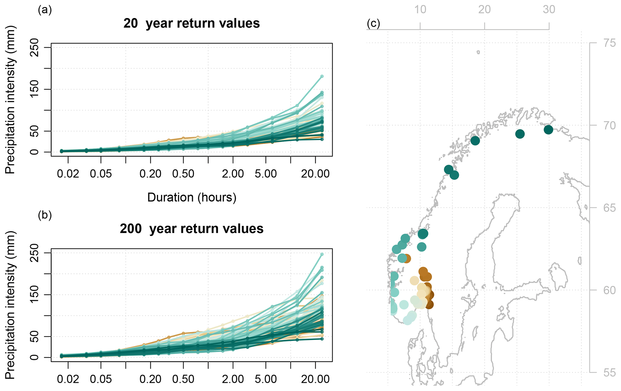
Figure 1Return values for 74 Norwegian stations for the (a) 20- and (b) 200-year return periods. The colours represent different locations shown in the map (c).
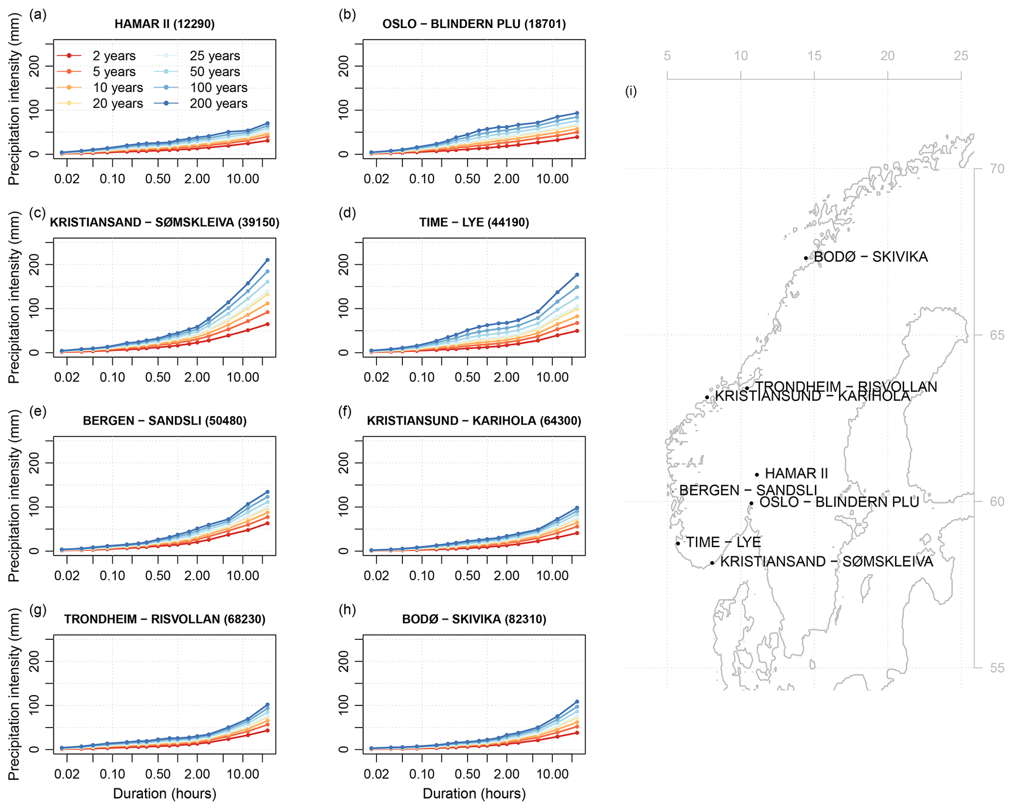
Figure 2IDF curves for (a) Hamar II, (b) Oslo – Blindern Plu, (c) Kristiansand – Sømskleiva, (d) Time – Lye, (e) Bergen – Sandsli, (f) Kristiansund – Karihola, (e) Trondheim – Risvollan, and (g) Bodø – Skivika. The locations of the stations are shown on a map in panel (i). The colour scale represents the various return periods, from 2 to 200 years, as described in the legend in panel (a).
Daily mean precipitation (pr) and air temperature at 2 m (t2 m) data were downloaded from the Norwegian Meteorological Institute (https://frost.met.no, last access: 29 April 2022), from the same stations as the IDF data or those closest available. Only stations with at least 10 years of data within the period 1970–2020 were included in the analysis. The availability of daily precipitation and temperature data is shown in the Supplement (Fig. S1). All IDF stations had daily precipitation data, but only 17 of the 74 stations had available temperature data. At the stations that did not, the distance to the nearest station with temperature data was on average 6.3 km and at most 25 km. Due to limited spatial coverage of the observational network, the same temperature data were assigned to multiple IDF stations in some cases (12 stations were assigned to multiple IDF stations, 46 were used only once). The multiple assignments occurred primarily in the more densely populated parts of the country (around Oslo, Trondheim, and Stavanger), where there are many observational stations in a relatively small area.
2.2 Principal component analysis of the IDF curves
Principal component analysis (PCA) was applied to the IDF curves through singular value decomposition (SVD) (Jolliffe, 1986; Jolliffe and Cadima, 2016; Trefethen and Bau, 1997). This framework was based on the expression
where the matrix X contains the IDF curves, i.e. return values for various return periods and durations at each location; U is a matrix holding eigenvectors, which can be interpreted as shapes of IDF curves; Λ is a diagonal matrix holding the eigenvalues; and V represents the principal components (PCs) containing weights for the different geographical locations.
The purpose of the PCA was to reduce the complexity of the IDF data while preserving as much variability as possible. The procedure finds new variables that are linear functions of the original data, where the new variables (PCs) are uncorrelated with each other, and the variance is successively maximised, meaning that the leading PC describes the dominant pattern, and each successive mode represents a smaller and smaller portion of the variance. The original IDF curves can thus be reproduced by combining a few of the leading PCs, eigenvectors, and eigenvalues with little loss of information.
We consider several criteria for assessing the number m of PCs that needs to be retained in order to represent most of the information: (i) set m to the smallest value for which the total cumulative explained variance exceeds a given percentage, for example, 80 % or 90 %. (The explained variance can be calculated from the eigenvalues λ.) (ii) Using a Scree diagram where the eigenvalues are plotted against their rank, identify an “elbow” (a bend in the curve where the slope goes from steep to shallow) and retain the eigenvalues to the left of this point (Cattell, 1966). (iii) An approach suggested by Ali et al. (1985) is to calculate the correlation between the original variables and the PCs and set m to one less than the first PC for which there are no correlation coefficients that are statistically significantly different from zero. In our case, the “original variables” are the return values, which for each station was compared with the IDF shapes Ui for i∈ [1,10] (Eq. 1).
There are other more objective but also computationally demanding methods of selecting the number of PCs to retain, for example, based on cross-validation or bootstrapping, but these were not deemed necessary for our purposes. Based on the criteria above, we focused primarily only on the two leading PCs in most of the analysis and statistical modelling of this study (see discussion in Sect. 3.1).
2.3 Statistical modelling
Statistical relationships were established between the two leading PCs of the IDF curves, which represent the dominant spatial patterns of the data, and a set of geographical and meteorological predictors: the wet-day mean precipitation in the warm season (April–September) and cold season (October–March), μwarm and μcold; the wet-day frequency in the warm season and cold season, and ; the temperature in the summer season (June–August), ; the latitude; the altitude, and the minimum distance to the coast (docean). These predictors describe both the cold-season precipitation regime in Norway, primarily dominated by stratiform precipitation associated with low-pressure systems, and the warm-season precipitation regime, which to a larger degree is regulated by convective processes. The summer temperature was included because it is closely linked to the convective environment.
The statistical model can be described as follows:
where Vi is the ith spatial pattern obtained by PCA of the IDF curves (Eq. 1); c0,i is the intercept; and c1,i, c2,i, …, cN,i are the coefficients associated with the predictors p1, p2, …, pN for principal component i∈ [1,2].
The estimated principal components were then combined with the corresponding eigenvectors and eigenvalues:
where the matrix contains the estimated IDF curves; is a matrix with the estimated eigenvectors and (Eq. 2); and U1,2 and Λ1,2 are matrices holding the first two leading eigenvectors and eigenvalues, respectively (a subset of U and Λ from Eq. 1).
Model fitting was performed by Bayesian linear regression, using the R package “BAS” (see Clyde et al., 2011, 2018, Chap. 6–8). A Markov chain–Monte Carlo (MCMC) resampling method was used for stochastic exploration of the model space. The number of predictors was reduced by applying the median probability model (MPM) rule: including only variables with a marginal posterior inclusion probability (pip) of at least 0.5 (Barbieri and Berger, 2004).
2.4 Evaluation of results
2.4.1 Cross-validation
To evaluate model skill, a leave-one-out cross-validation was performed in which the predictand and predictor data of one station were excluded from model calibration. The statistical model was subsequently applied to the climatological and geographical data of the excluded station to estimate return values. This procedure was repeated so that independent estimates of the return values were obtained for all stations. The root-mean-square error (RMSE) and relative RMSE between the original return values and independent estimates obtained through cross-validation were then calculated as described in Appendix A.
2.4.2 Confidence intervals
Confidence intervals of the estimated return values, , were calculated based on the standard errors of the estimated PCs, and , which were provided as output of the Bayesian linear regression function. Since the principal components are orthogonal, the error propagation equation for linear combinations (Ku, 1966) simplifies to
where is the total error of the estimated return values, ; is the standard errors of the ith principal component, Vi; and Ui and Λi are the ith eigenvector and eigenvalue, respectively (see Eqs. 1 and 3).
2.5 Comparison with other methods
The IDF curves estimated with Bayesian inference of principal components, as described above, were compared with the simple approximate formula for estimating return values derived by Benestad et al. (2021):
where XL is the return value (unit: mm) for the duration L (unit: h); μ (unit: mm d−1) and fw (unit: fraction of days) are the wet-day mean precipitation and wet-day frequency, respectively, calculated from daily precipitation observations; and α and ζ are empirical correction factors that vary with the return period τ (unit: years). The value of α varies linearly with the logarithm of the return period according to . Values of ζ have been fitted for a range of return periods (0.4251593, 0.4185929, 0.4161947, 0.4147515, 0.4144257, 0.4137387, 0.4134449, and 0.4134594 for 2-, 5-, 10-, 20-, 25-, 50-, 100-, and 200-year return periods) and are obtained by interpolation for other values of τ. Equation (5) has been implemented in the R package “esd” (Benestad et al., 2015), where it is available as the function day2IDF().
3.1 PCA of the IDF curves
As mentioned earlier, principal component analysis was applied to the IDF statistics as described in Sect. 2.2 with the purpose of reducing the dimensionality of the data. The five leading principal components explained 74 %, 9 %, 3 %, 3 %, and 2 % of the variability of the IDF statistics, respectively. At least two PCs need to be retained in order to explain 80 % of the variance or five PCs for the cumulative explained variance to exceed 90 %. In the Scree diagram (Fig. 3a), an elbow was identified between V2 and V3, suggesting that the two leading PCs represent the most relevant information. However, based on the comparison between the IDF shapes Ui and the original return values, statistically significant correlations (with p<0.01) were found for i∈ [1,4], suggesting that the leading four PCs all hold information of some importance.
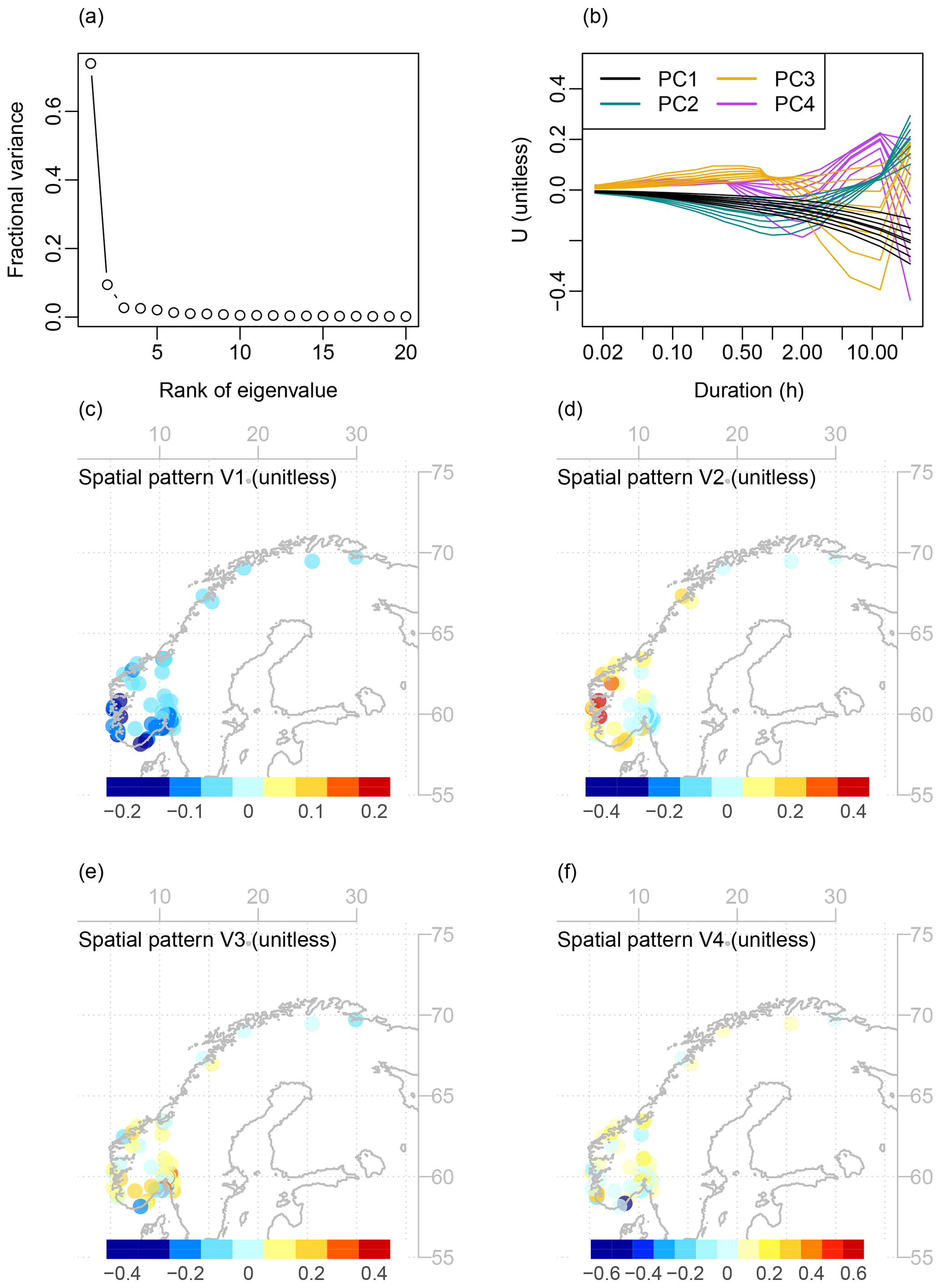
Figure 3Summary figure describing different aspects of the PCA of the IDF curves. Panel (a) shows a Scree diagram with the rank of the eigenvalues (abscissa) plotted against the explained variance (ordinate). Panel (b) displays the IDF shapes (U in Eq. 1) associated with the leading four principal components, and panels (c, d, e, f) show the associated spatial patterns (V in Eq. 1) for PC1, PC2, PC3, and PC4, respectively.
The spatial pattern associated with the first principal component, V1, was characterised by a west–east and south–north gradient, with a strong contrast between the western and southern coasts of Norway on the one hand and the inland and middle–northern Norway on the other hand (Fig. 3c). The values of V1 were of the same sign (negative) at all stations, meaning that it described a pattern with positive correlations among all stations. The second principal component, V2, spanned both positive and negative values and displayed a gradient from the inland region, where V2<0 at most stations, to the western and southern coast, where V2>0 (Fig. 3d). The higher-order spatial patterns had less coherent spatial structures, also spanning positive and negative values (Fig. 3e and f).
A reconstruction of the IDF statistics (Fig. S8) from only the first PC showed that it determined the basic slope and level of the IDF curves. The second PC altered the curvature: in the stations where V2>0, the second PC made the IDF curve more convex, i.e. decreased return values for short to intermediate durations and increased them for long durations. In stations where V2<0, PC2 had the opposite influence, making the curve more flat or concave instead. This can also be understood by looking directly at the IDF shapes (U in Eq. 1) associated with the leading principal components, displayed in Fig. 3b. For U1, the curves decreased smoothly with increasing duration and return period, which makes sense as V1 was negative at all stations. For U2, there was a maximum at 24 h duration and a minimum around 1–2 h duration. This explains why positive values of V2 give more convex shapes and positive values more concave. The higher-order modes (U3 and U4) had shapes with local minima and maxima at various durations, but because of their small eigenvalues (Fig. 1a) they had little visible influence on the IDF curves, only slightly tweaking their shapes.
3.2 Statistical modelling
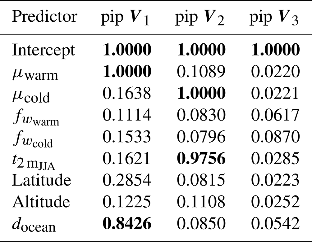
Statistical models were fitted for the first two principal components of the IDF statistics, V1 and V2, using Bayesian linear regression as described in Sect. 2.3. The posterior inclusion probability of the coefficients suggested that the most important predictors for V1 were μwarm and docean and for V2 μcold and (Table 1; Figs. S9–S10). An attempt was made to fit a model for V3, but no predictors could be identified that gave a better prediction than a model consisting of only the intercept (Fig. S11). As no model could be found for V3, and previous analysis indicated that it had a limited influence on the IDF shapes, it was excluded from further statistical modelling and analysis. The models for V1 and V2 were refitted with the selected predictors to keep the size of the predictor set small and reduce the risk of over-fitting (Wilks, 1995).
Table 1Marginal posterior inclusion probability (pip) of the coefficients for different predictor variables in the statistical models for the three leading principal components of the IDF curves, V1, V2 and V3. A pip higher than 0.5 (shown in bold font) indicates that the coefficient is included in the Median Probability Model (MPM), which is the model selection approach used in this study. The included predictor variables are the wet-day mean precipitation in the warm and cold season (μwarm, μcold), the wet-day frequency in the warm and cold season (, ), the mean summer temperature (), the latitude, the altitude, and the distance to the ocean (docean).
Figures 4 and S13 demonstrate the effect of the predictor variables on the estimated 200-year return values for the station Hamar II. Similar results were seen at other stations and for other return periods. The two predictors included in the model of V1 (μwarm and docean) had the most notable influence on the basic shape and level of the IDF curves. An increase in μwarm or decrease in docean gave an overall increase in return values but more for long durations than short durations, hence increasing the slope of the IDF curves (Fig. 4a and b). A decrease in μwarm or increase in docean had the opposite effect, decreasing return levels and the slope of the curves. The predictor variables that were involved in the model of V2 (μcold, and ) altered the curvature of the estimated IDF curves. An increase in μcold or decrease in lowered return values for low to intermediate durations (<6 h) and increased return values for long durations (>6 h), resulting in a more concave upwards curve (Fig. 4c and d). A decrease in μcold or increase in had the opposite effect, resulting in a more convex downward curve.
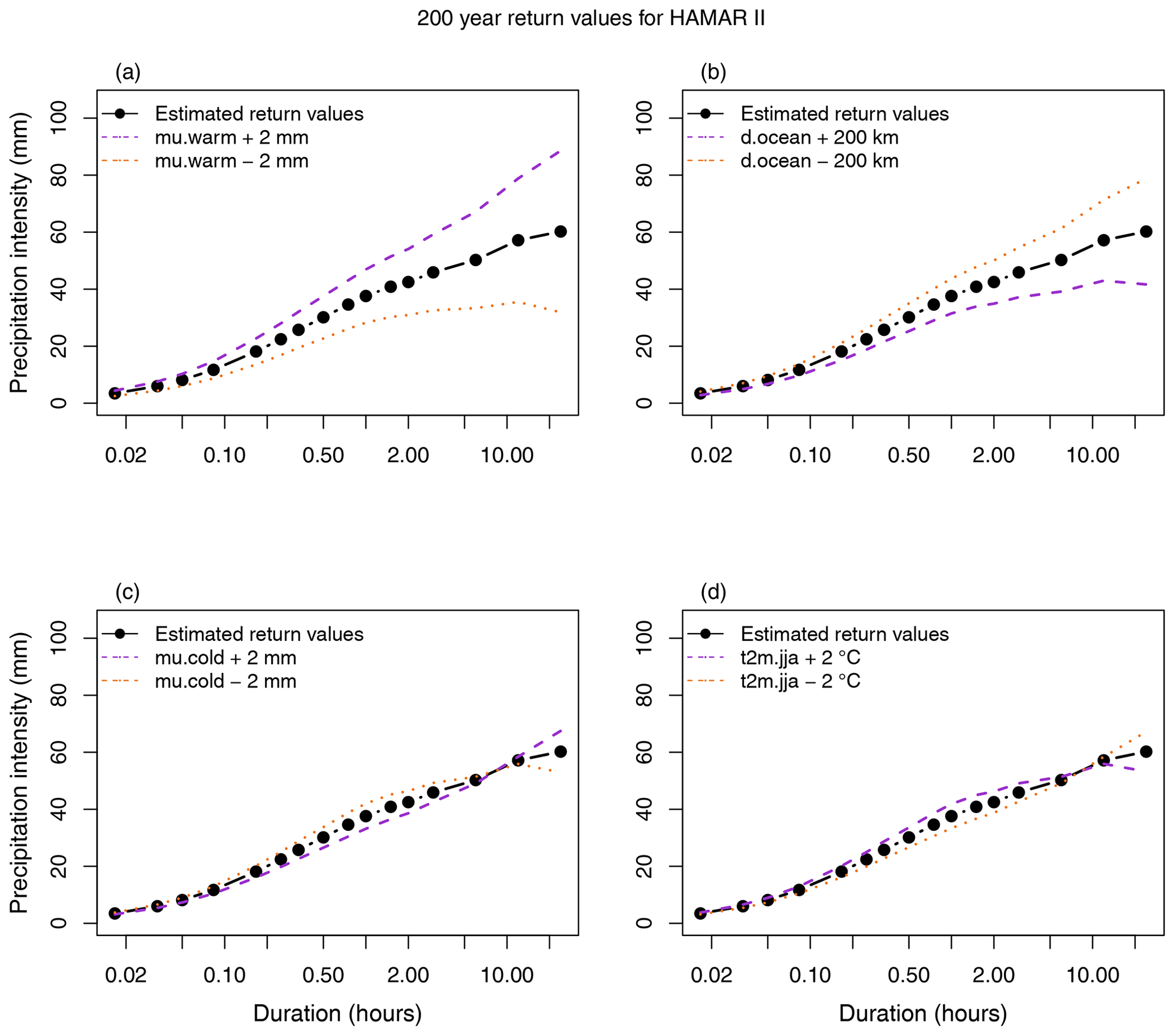
Figure 4Demonstration of the effect of the model parameters (a) μwarm, (b) docean, (c) μcold, and (d) on the estimated 200-year return values for the station Hamar II. The plots show return values estimated with parameter values from observations (black lines and dots), as well as with increased (dashed purple lines) and decreased (dotted orange lines) parameter values.
A new set of IDF curves was constructed by combining the predicted principal components and with the corresponding eigenvectors and eigenvalues (Eq. 3). Cross-validation (Sect. 2.4.1) showed that the estimated return values were robust in the sense that they were very similar whether a station was included in model fitting or not: comparing return values estimated by models tuned with all data and by cross-validation, the RMSE was only 0.9 mm or 3 % in relative terms (see examples in Fig. S14). At the eight example stations, the confidence intervals of the original IDF statistics and of the estimated return values overlapped for all durations and return periods (Fig. 5). The deviation between estimated and original return values was generally larger in stations with more steep and curved slopes (i.e. large differences between short and long durations as in Fig. 5c, d, and e) compared to the stations with flatter IDF curves.
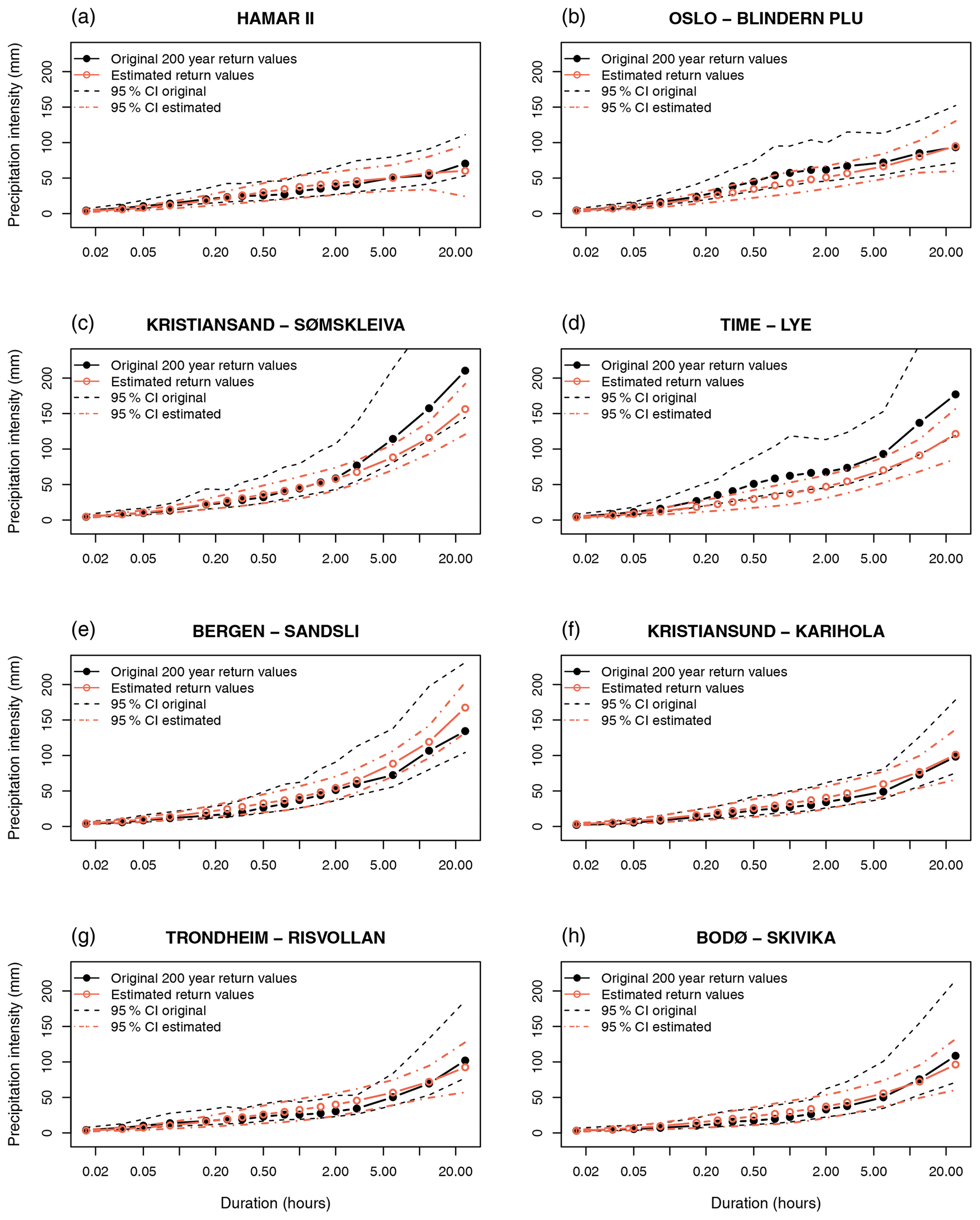
Figure 5Estimated 200-year return values for eight example stations: (a) Hamar II, (b) Oslo – Blindern Plu, (c) Kristiansand – Sømskleiva, (d) Time – Lye, (e) Bergen – Sandsli, (f) Kristiansand – Karihola, and (g) Bodø – Skivika. The plots show the original IDF curves (black) as well as return values estimated by Bayesian inference as described in this paper (coral). Dashed lines show the confidence interval (2 standard errors) of the original (dashed black) and estimated (dashed coral) IDF curves.
A comparison between the original return values and values estimated from the two leading original PCs (Fig. 6a and b) showed that there was some loss of information from discarding higher-order modes of variability, but the RMSE was rather low (2.3 mm or, in relative terms, 9 %) and the PCA added no bias. The Bayesian statistical modelling of the two leading PCs (Fig. 6b) added uncertainty to the return value estimates (RMSE = 5.9 mm, 23 %) but was still more precise than the simple equation by Benestad (RMSE = 9 mm; 35 %) (Figs. 6c and S19). There was no obvious spatial pattern in the RMSE of the return values obtained by the Bayesian approach (not shown here; see Fig. S20). For the simple formula, the largest biases occurred for short return periods, for which there was a tendency to overestimate the return values, while there was little bias for longer return periods. For the Bayesian modelling of the first two PCs, there was a tendency to underestimate high return values, and the bias was similar for all return periods. The Bayesian modelling approach was notably better for low to medium return values (<100 mm), but the discrepancies associated with the two methods were of similar magnitude for higher return values. The improved representation of the IDF statistics by the Bayesian modelling was not surprising since it involved an optimisation process that found the best slope and curvature of the IDF shapes, whereas the estimates based on the simple formula only used the two parameters μ and fw. In the simple formula, the shapes of the IDF curves were fixed in terms of a fractal describing inter-scalar dependencies. Nevertheless, the two different strategies gave somewhat similar results, albeit with substantial scatter.
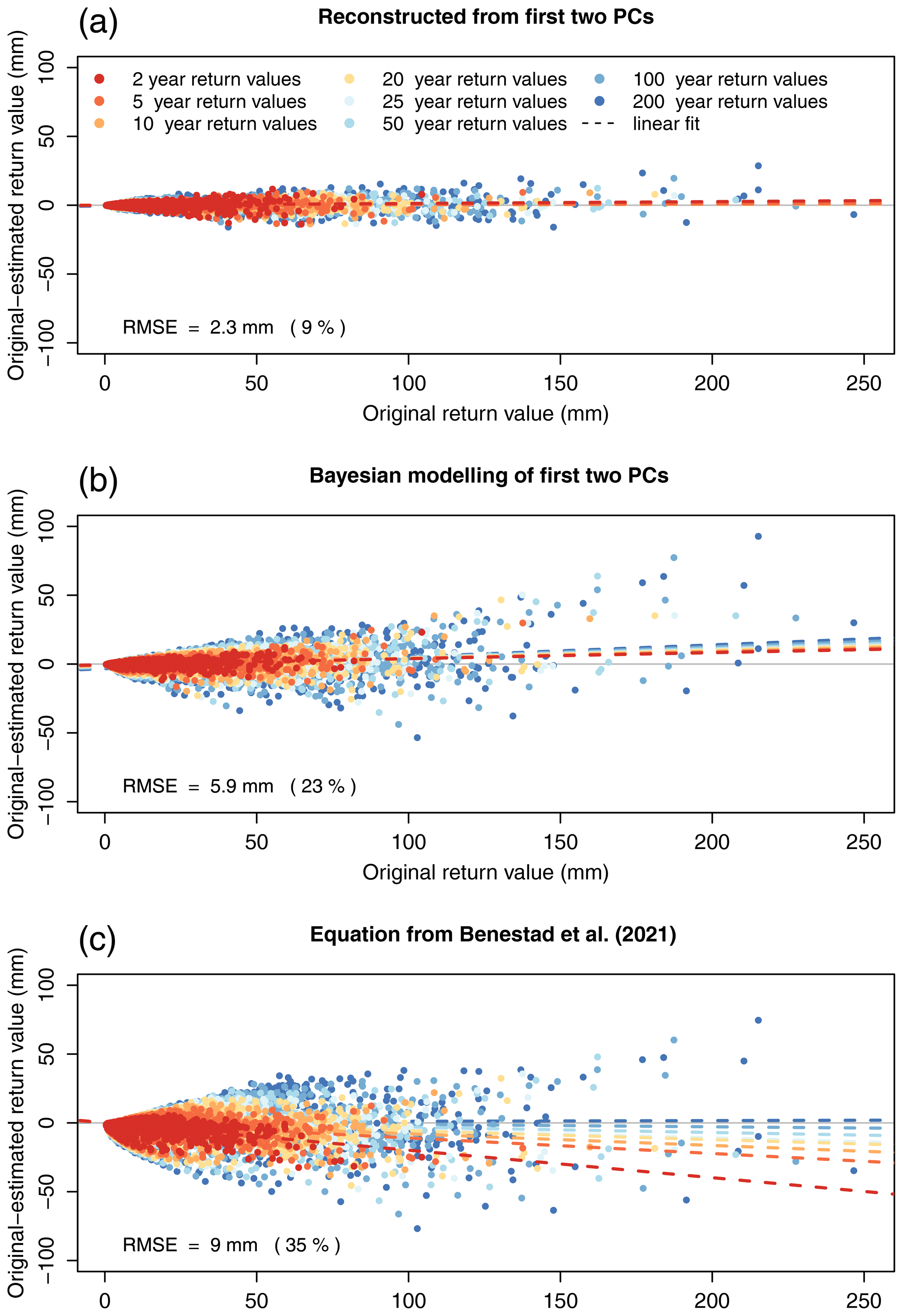
Figure 6Original return values plotted against the error of the estimated return values (original–estimated) calculated (a) from the two leading PCs of the original return values, (b) by Bayesian modelling of the two leading PCs of the return values, and (c) using the equation presented in Benestad et al. (2021). The colours represent different return periods (see legend in panel a). Points show individual return values, and dashed lines show linear regressions for each return period. The RMSE and relative RMSE of the estimated and original return values are displayed in the lower-left corner of each panel.
New IDF curves were generated by applying the statistical models to meteorological and geographical data for 240 stations in Norway, including Svalbard and Jan Mayen (Fig. 7). Many of these stations lack long time series of high-quality sub-daily precipitation data, and thus IDF curves cannot be calculated by ordinary measures.
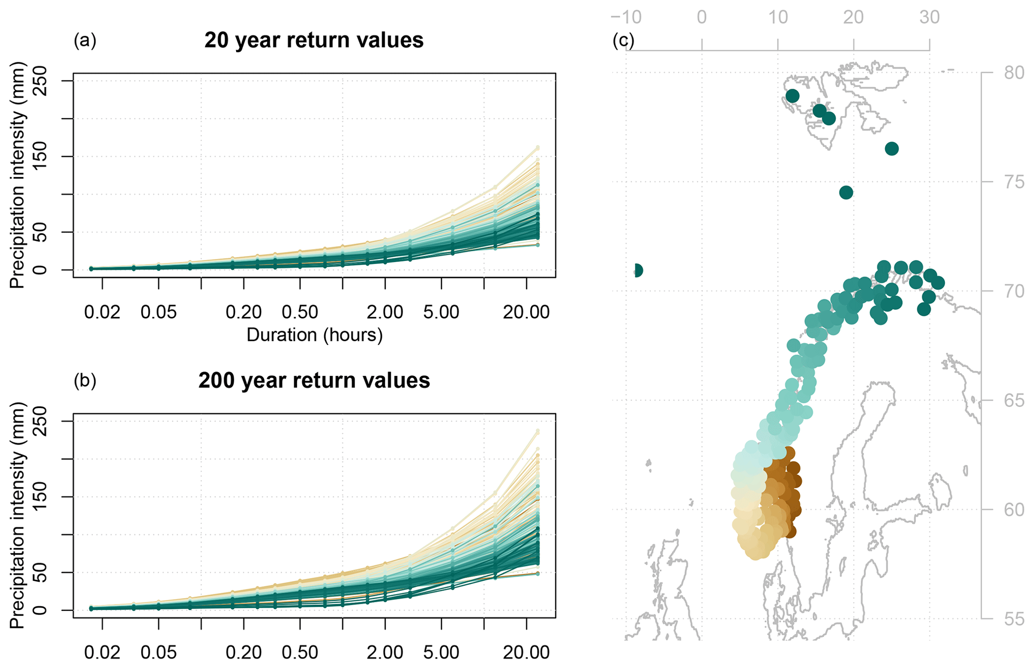
Figure 7Estimated return values for 240 Norwegian stations for the (a) 20-year and (b) 200-year return period, calculated using statistical models applied to temperature and precipitation data that were not used for model calibration. The map (c) shows which locations the colours in the return value plots represent.
Comparing the original return values (Figs. 1 and S3) to the estimated values (Figs. 7 and S22), the estimated IDF curves are smoother than the original curves. There are obvious regional differences in the shapes of the IDF curves: towards the west coast, the IDF curves reach the highest values, and the curvature tends to be strong (i.e., a large difference between the intensity of short and long durations) compared to stations inland and up north. At northern locations, the IDF curves are lower with a moderate slope. These regional differences were more emphasised in the estimated return values. Most notably, in the southeast region (south of 62∘ N, east of 9∘ E), the range of estimated return values was considerably more narrow compared to the original IDF data, even though the estimated values represent more stations covering a larger area.
The regression results presented in Table 1 and Fig. 4 indicated that the mean precipitation intensity in the warm season is connected to increased intensity over all timescales examined, whereas a similar increase in the cold season suggested reduced short-term intensity but increased long-term intensity. A similar increase over all timescales in the warm season is consistent with Eq. (5) , assuming a constant value for ζ, but the deviation from this in winter may suggest that ζ is not necessarily constant. The difference in seasonal response is likely related to the dominance of different precipitation-generating processes: stratiform in winter and convective in summer. It could also possibly be connected to the warm and cold initiation of precipitation (Rogers and Yau, 1989). The locations with intense winter precipitation, which tend to have high return values for long durations and relatively low return values for shorter durations, are found along the west coast (Figs. 1, 7, S3 and S22). The climate of this region is characterised by the North Atlantic storm tracks, bringing a steady stream of cyclones that often meet land here in autumn and winter, giving rise to heavy-precipitation events with a long duration, and a relatively cold climate in summer, which is not conducive to convection. Further inland, the heavy-precipitation events often occur in summer as a result of convection, which is in line with the relatively high return values for shorter durations. Furthermore, there is a degree of orographically forced precipitation along the mountain ranges. The influence of the distance to the ocean and temperature in summer (Fig. 4) also supports this picture, with the curvature of the IDF curves decreasing with increasing and docean.
An advantage of the proposed method, applying PCA to the IDF data, is that all durations and return periods are considered together. This is not only computationally efficient but also reduces the influence of uncertain or erroneous individual return levels. There are also some potential pitfalls with this approach. First of all, only the first two PCs could be modelled, which could have too much of a smoothing effect on the IDF curves. There could also be nonlinear effects that were not captured by the linear models, which could result in underestimated variations in the estimated PCs. The quality of the estimated return levels was limited by the quality of the IDF data that they were based on. A different set of IDF statistics would likely result in statistical models with similar predictors and coefficients, but the PCA and ultimately the estimated IDF curves would be defined by the shape of the IDF data.
IDF statistics tend to have large uncertainties attached to them, as illustrated by the confidence intervals in Fig. 5. It can therefore be difficult to evaluate what constitutes a skilful estimation of return values. Although the IDF statistics used in this paper (Lutz et al., 2020) are referred to as the “original” return values, they too were estimated and not directly observed. Is it enough that the confidence intervals of the two estimates overlap? If so, the regionalisation approach presented here is “good enough”. On the other hand, the confidence intervals of the PCA-based estimates are for sure underestimated because they represent only the distribution of the Bayesian regression coefficients, without taking into account the uncertainties of the IDF statistics or climatological information that went into the modelling.
A more direct evaluation of model skill might be between the original return values (that were also obtained as median values of a distribution; see Lutz et al., 2020) and the confidence intervals of the estimated return values. Using this metric, the statistical modelling was successful at most but not all stations. For the 24 h duration and 200-year return period, which is where the largest discrepancies occurred (Fig. 6b), there were five stations at which the original return values were outside of the confidence interval of the estimated return values (Fig. S15): four stations along the southern coast of Norway, at which the return values were underestimated compared to the original values, and one station on the west coast, where the return value is overestimated instead. A closer examination revealed that at two of the stations where the return values were underestimated (Grimstad – Hia and Time – Lye), the problem could be traced to the discarding of higher-order PCs, as PC4 had a notable influence on the shape of the IDF curves (not shown). At the other stations with large discrepancies, the explanation was not as easy to find but likely connected to the Bayesian regression.
Expanding IDF curves from gauged to ungauged locations or from current to future periods leans on the assumption that the transfer functions are stationary and the climate data that go into the analyses are representative of the location/period that they are associated with. This is not always true. If the reference period is shorter than the relevant cycles of natural climate variability or if there is a trend or large interannual variability, the outcome will likely be sensitive to the precise period of the input data. Dyrrdal et al. (2021) found significant changes in heavy precipitation in the Nordic–Baltic region and concluded that return level calculations were sensitive to the time period of available data. One strategy, suggested by Fadhel et al. (2017), is to investigate and quantify the uncertainty related to this issue by repeating the analyses with input data from varying periods. To test the robustness of the proposed method, we applied the statistical models to climatological data from two different periods (1970–1995 and 1995–2020) at 36 stations with long, complete observational records. The results (Fig. S24) showed that for long durations, the estimated return values could differ as much as 10–20 mm at some stations depending on the reference period. This uncertainty should ideally have been included in the confidence intervals of the estimated IDF curves, but short observational records made it difficult to do this at most locations. In future studies, additional sources of information such as high-resolution gridded products may be helpful to fill in the gaps of the observational network in space and time.
Given that the IDF statistics in Norway are estimated for each duration separately and often based on short time series (Lutz et al., 2020), the smoother shapes of the IDF curves estimated by PCA-based Bayesian regression may, at some stations, be more representative of the precipitation climate than the original return values which they are based on. Hence, the PCA-based approach with Bayesian inference can be regarded as another “tool” together with the traditional approach for estimating IDFs and the simple formula proposed by Benestad et al. (2021). They are based on different assumptions and have different strengths and weaknesses, and together they can capture salient information and smooth over errors from single sites, as the different approaches to predicting IDF curves are based on independent methods, for example, modelling the return values (Dyrrdal et al., 2015), estimating future IDF curves based on changes in the precipitation intensity (Zhu et al., 2012), and downscaling rainfall intensity with respect to timescale (Rodríguez et al., 2014; Benestad et al., 2021).
As an alternative to PCA, we tried using a weighted set of polynomials to represent the shapes of the IDF curves, fitting return values against time intervals (Fig. S6). This method was not successful. First- and second-order polynomials were not a good fit, and higher-order polynomials, while fitting the data reasonably well for the time intervals for which return value data were available, had wiggly shapes with local minima and maxima that did not make sense as IDF curves.
One interesting question is how to use the IDF modelling approach presented here in the context of climate change projections. For the case of Norway, the key variables expected to change are μwarm, μcold, and . By downscaling them, statistically or dynamically, we may be able to infer changes in the IDF through predicting new values for the PCs, assuming that their shapes will be valid in a future climate and the calibrated dependency holds. One limitation is our ability to get reliable estimates for the wet-day mean precipitation in the future, which can be challenging in the case of empirical–statistical downscaling. We can also use this approach to provide hypothetical IDF curves for stress testing (Benestad et al., 2019a). Other caveats may be that these results only apply to Norway and that similar analyses for different regions may find that different factors are important for the shape of the IDF curves. We expect that the shapes of the IDF curves depend on physical aspects such as mesoscale convection, synoptic frontal systems and cyclones, orographic precipitation, and atmospheric rivers and that they will be sensitive to changes in their occurrence relative to each other.
We obtained predictions of the shape of IDF curves in Norway with Bayesian inference applied to a PCA representation of the IDF data and conclude that it provides a useful strategy that can be utilised for regionalisation and downscaling of future climate projections.
Statistical measures of the discrepancy between original return values x and fitted values y were calculated as follows:
The data code used to carry out this analysis is available in an R Markdown document provided in the Supplement. The daily precipitation and temperature data used in this paper are publicly available at https://frost.met.no (last access: 29 April 2022), which is an API that provides free access to MET Norway’s historical archive of quality-controlled climate and weather data, and the IDF statistics are available on request from the authors.
The supplement related to this article is available online at: https://doi.org/10.5194/hess-27-3719-2023-supplement.
KMP and REB contributed to the data analysis. JL supplied the IDF data. All authors participated in writing the manuscript.
The contact author has declared that none of the authors has any competing interests.
Publisher’s note: Copernicus Publications remains neutral with regard to jurisdictional claims in published maps and institutional affiliations.
This work was supported by the Norwegian Meteorological Institute and the KlimaDigital project.
This research has been supported by the Norges Forskningsråd (grant no. 281059).
This paper was edited by Dominic Mazvimavi and reviewed by two anonymous referees.
Ali, A., Clarke, G. M., and Trustrum, K.: Principal component analysis applied to some data from fruit nutrition experiments, Statistician, 34, 365–369, 1985. a
Barbieri, M. M. and Berger, J. O.: Optimal predictive model selection, Ann. Stat., 32, 870–897, 2004. a
Benestad, R. E.: Implications of a decrease in the precipitation area for the past and the future, Environ. Res. Lett., 13, 044022, https://doi.org/10.1088/1748-9326/aab375, 2018. a
Benestad, R. E., Mezghani, A., and Parding, K. M.: Esd V1.0, Zenodo [code], https://doi.org/10.5281/ZENODO.29385, 2015. a
Benestad, R. E., Parding, K., Mezghani, A., Dobler, A., Landgren, O., Erlandsen, H., Lutz, J., and Haugen, J.: Stress Testing for Climate Impacts with “Synthetic Storms”, Eos, 100, https://doi.org/10.1029/2019EO113311, 2019a. a
Benestad, R. E., Parding, K. M., Erlandsen, H. B., and Mezghani, A.: A simple equation to study changes in rainfall statistics, Environ. Res. Lett., 14, 084017, https://doi.org/10.1088/1748-9326/ab2bb2, 2019b. a
Benestad, R. E., Lutz, J., Dyrrdal, A. V., Haugen, J. E., Parding, K. M., and Dobler, A.: Testing a simple formula for calculating approximate intensity-duration-frequency curves, Environ. Res. Lett., 16, 044009, https://doi.org/10.1088/1748-9326/abd4ab, 2021. a, b, c, d, e, f, g
Benestad, R. E., Lussana, C., Lutz, J., Dobler, A., Landgren, O., Haugen, J. E., Mezghani, A., Casati, B., and Parding, K. M.: Global hydro-climatological indicators and changes in the global hydrological cycle and rainfall patterns, PLOS Climate, 1, e0000029, https://doi.org/10.1371/journal.pclm.0000029, 2022. a
Burn, D. H.: A framework for regional estimation of intensity-duration-frequency (IDF) curves: REGIONAL ESTIMATION OF INTENSITY-DURATION-FREQUENCY (IDF) CURVES, Hydrol. Process., 28, 4209–4218, https://doi.org/10.1002/hyp.10231, 2014. a
Cattell, R. B.: The Scree Plot Test for the Number of Factors, Multivar. Behav. Res., 1, 140–161, https://doi.org/10.1207/s15327906mbr0102_10, 1966. a
Chandra, R., Saha, U., and Mujumdar, P.: Model and parameter uncertainty in IDF relationships under climate change, Adv. Water Res., 79, 127–139, https://doi.org/10.1016/j.advwatres.2015.02.011, 2015. a
Clyde, M., Ghosh, J., and Littman, M. L.: Bayesian Adaptive Sampling for Variable Selection and Model Averaging, J. Comput. Graph. Stat., 20, 80–101, https://doi.org/10.1198/jcgs.2010.09049, 2011. a
Clyde, M., Çetinkaya Rundel, M., Rundel, C., Banks, D., and Huang, L.: An Introduction to Bayesian Thinking, A Companion to the Statistics with R Course, https://statswithr.github.io/book/ (last access: 17 October 2023), 2018. a
Donat, M. G., Alexander, L. V., Herold, N., and Dittus, A. J.: Temperature and precipitation extremes in century‐long gridded observations, reanalyses, and atmospheric model simulations, J. Geophys. Res.-Atmos., 121, 11174–11189, https://doi.org/10.1002/2016JD025480, 2016. a
Dyrrdal, A. V., Lenkoski, A., Thorarinsdottir, T. L., and Stordal, F.: Bayesian hierarchical modeling of extreme hourly precipitation in Norway: Modeling extreme hourly precipitation in Norway, Environmetrics, 26, 89–106, https://doi.org/10.1002/env.2301, 2015. a, b, c
Dyrrdal, A. V., Olsson, J., Médus, E., Arnbjerg-Nielsen, K., Post, P., Aņiskeviča, S., Thorndahl, S., Førland, E., Wern, L., Mačiulytė, V., and Mäkelä, A.: Observed changes in heavy daily precipitation over the Nordic-Baltic region, J. Hydrol., 38, 100965, https://doi.org/10.1016/j.ejrh.2021.100965, 2021. a, b
Eldardiry, H., Habib, E., and Zhang, Y.: On the use of radar-based quantitative precipitation estimates for precipitation frequency analysis, J. Hydrol., 531, 441–453, https://doi.org/10.1016/j.jhydrol.2015.05.016, 2015. a, b
Fadhel, S., Rico-Ramirez, M. A., and Han, D.: Uncertainty of Intensity–Duration–Frequency (IDF) curves due to varied climate baseline periods, J. Hydrol., 547, 600–612, https://doi.org/10.1016/j.jhydrol.2017.02.013, 2017. a, b
Fauer, F. S., Ulrich, J., Jurado, O. E., and Rust, H. W.: Flexible and consistent quantile estimation for intensity–duration–frequency curves, Hydrol. Earth Syst. Sci., 25, 6479–6494, https://doi.org/10.5194/hess-25-6479-2021, 2021. a
Field, C., Barros, V., Stocker, T. F., Qin, D., Dokken, D. J., Ebi, K. L., Mastrandrea, M. D., Mach, K. J., Plattner, G.-K., Allen, S. K., Tignor, M., and Midgley, P. M. (Eds.): Managing the Risks of Extreme Events and Disasters to Advance Climate Change Adaptation, in: A Special Report of Working Groups I and II of the Intergovernmental Panel on Climate Change, Cambridge University Press, Cambridge, UK, and New York, NY, USA, https://doi.org/10.1017/CBO9781139177245, 2012. a
Gado, T. A., Hsu, K., and Sorooshian, S.: Rainfall frequency analysis for ungauged sites using satellite precipitation products, J. Hydrol., 554, 646–655, https://doi.org/10.1016/j.jhydrol.2017.09.043, 2017. a
IPCC: Climate Change 2021: The Physical Science Basis, Contribution of Working Group I to the Sixth Assessment Report of the Intergovernmental Panel on Climate Change, Cambridge University Press, https://www.ipcc.ch/report/ar6/wg1/ (last access: 17 October 2023), 2021. a, b
Jolliffe, I. T.: Principal Component Analysis, Springer Series in Statistics, Springer, https://doi.org/10.1007/0-387-22440-8_13, 1986. a
Jolliffe, I. T. and Cadima, J.: Principal component analysis: a review and recent developments, Philos. T. R. Soc. A, 374, 20150202, https://doi.org/10.1098/rsta.2015.0202, 2016. a
Koutsoyiannis, D., Kozonis, D., and Manetas, A.: A mathematical framework for studying rainfall intensity-duration-frequency relationships, J. Hydrol., 206, 118–135, https://doi.org/10.1016/S0022-1694(98)00097-3, 1998. a
Kreklow, J., Tetzlaff, B., Burkhard, B., and Kuhnt, G.: Radar-Based Precipitation Climatology in Germany – Developments, Uncertainties and Potentials, Atmosphere, 11, 217, https://doi.org/10.3390/atmos11020217, 2020. a
Ku, H. H.: Notes on the use of propagation of error formulas, J. Res. Natl. Bur. Stand., 70C, 263–237, https://doi.org/10.6028/jres.070C.025, 1966. a
Lima, C. H., Kwon, H.-H., and Kim, Y.-T.: A local-regional scaling-invariant Bayesian GEV model for estimating rainfall IDF curves in a future climate, J. Hydrol., 566, 73–88, https://doi.org/10.1016/j.jhydrol.2018.08.075, 2018. a
Lutz, J., Grinde, L., and Dyrrdal, A. V.: Estimating Rainfall Design Values for the City of Oslo, Norway – Comparison of Methods and Quantification of Uncertainty, Water, 12, 1735, https://doi.org/10.3390/w12061735, 2020. a, b, c, d
Mailhot, A., Duchesne, S., Caya, D., and Talbot, G.: Assessment of future change in intensity–duration–frequency (IDF) curves for Southern Quebec using the Canadian Regional Climate Model (CRCM), J. Hydrol., 347, 197–210, https://doi.org/10.1016/j.jhydrol.2007.09.019, 2007. a
Marra, F., Morin, E., Peleg, N., Mei, Y., and Anagnostou, E. N.: Intensity–duration–frequency curves from remote sensing rainfall estimates: comparing satellite and weather radar over the eastern Mediterranean, Hydrol. Earth Syst. Sci., 21, 2389–2404, https://doi.org/10.5194/hess-21-2389-2017, 2017. a
Olsson, J., Dyrrdal, A. V., Médus, E., Södling, J., Aņiskeviča, S., Arnbjerg-Nielsen, K., Førland, E., Mačiulytė, V., Mäkelä, A., Post, P., Thorndahl, S. L., and Wern, L.: Sub-daily rainfall extremes in the Nordic-Baltic region, Hydrol. Res., 53, 807–824, https://doi.org/10.2166/nh.2022.119, 2022. a
Panziera, L., Gabella, M., Germann, U., and Martius, O.: A 12-year radar-based climatology of daily and sub-daily extreme precipitation over the Swiss Alps, Int. J. Climatol., 38, 3749–3769, https://doi.org/10.1002/joc.5528, 2018. a, b
Rodríguez, R., Navarro, X., Casas, M. C., Ribalaygua, J., Russo, B., Pouget, L., and Redaño, A.: Influence of climate change on IDF curves for the metropolitan area of Barcelona (Spain): Influence of climate change on IDF curves of Barcelona (Spain), Int. J. Climatol., 34, 643–654, https://doi.org/10.1002/joc.3712, 2014. a, b
Rogers, R. R. and Yau, M. K.: A Short Course in Cloud Physics, Pergamon Press, Oxford, 3 edn., https://doi.org/10.1175/1520-0477-70.9.1159a, 1989. a
Roksvåg, T., Lutz, J., Grinde, L., Dyrrdal, A. V., and Thorarinsdottir, T. L.: Consistent intensity-duration-frequency curves by post-processing of estimated Bayesian posterior quantiles, J. Hydrol., 603, 127000, https://doi.org/10.1016/j.jhydrol.2021.127000, 2021. a, b, c
Schilcher, U., Brandner, G., and Bettstetter, C.: Quantifying inhomogeneity of spatial point patterns, Comput. Netw., 115, 65–81, https://doi.org/10.1016/j.comnet.2016.12.018, 2017. a
Solomon, S., Quin, D., Manning, M., Chen, Z., Marquis, M., Averyt, K. B., Tignotr, M., and Miller, H. L. (Eds.): Contribution of Working Group I to the Fourth Assessment Report of the Intergovernmental Panel on Climate Change, in: Climate Change: The Physical Science Basis, Cambridge University Press, United Kingdom and New York, NY, USA, ISBN 978-0-521-70596-7, 2007. a
Sorteberg, A., Lawrence, D., Dyrrdal, A. V., Mayer, S., and Engeland, K.: Climatic changes in short duration extreme precipitation and rapid onset flooding – implications for design values, NCCS report 1/2018, Norwegian Climate Change Services, Oslo, Norway, https://www.met.no/kss/_/attachment/download/de0e8d57-236c-460b-8e94-23ce18274c1c:94752a62e18693c0ea185e9db24381d209c475af/exprecflood-final-report-nccs-signert.pdf (last access: 17 October 2023), 2018. a
Stocker, T. and Qin, D. (Eds.): Climate Change 2013: The Physical Science Basis. Contribution of Working Group I to the Fifth Assessment Report of the Intergovernmental Panel on Climate Change, WMO, UNEP, ISBN 978-1-107-66182-0, 2013. a
Trefethen, L. N. and Bau, D.: Numerical Linear Algebra, Society for Industrial and Applied Mathematics, 1 edn., https://doi.org/10.1137/1.9780898719574, 1997. a
Westra, S., Fowler, H. J., Evans, J. P., Alexander, L. V., Berg, P., Johnson, F., Kendon, E. J., Lenderink, G., and Roberts, N. M.: Future changes to the intensity and frequency of short-duration extreme rainfall: future intensity of sub-daily rainfall, Rev. Geophys., 52, 522–555, https://doi.org/10.1002/2014RG000464, 2014. a
Wilks, D. S.: Statistical Methods in the Atmospheric Sciences, Academic Press, Orlando, Florida, USA, ISBN 0-12-751965-3, 1995. a
Zhu, J., Stone, M. C., and Forsee, W.: Analysis of potential impacts of climate change on intensity–duration–frequency (IDF) relationships for six regions in the United States, J. Water Clim. Change, 3, 185–196, https://doi.org/10.2166/wcc.2012.045, 2012. a