Improving the quantification of climate change hazards by hydrological models: a simple ensemble approach for considering the uncertain effect of vegetation response to climate change on potential evapotranspiration

Almost no hydrological model takes into account that changes in evapotranspiration are affected by how vegetation responds to changing CO₂ and climate. This severely limits their ability to quantify the impact of climate change on evapotranspiration and, thus, water resources. As the simulation of vegetation responses is both complex and very uncertain, we recommend a simple approach to considering (in climate change impact studies with hydrological models) the uncertainty that the vegetation response causes with respect to the estimation of future potential evapotranspiration (PET). To quantify this uncertainty in a simple manner, we propose running the hydrological model in two variants: with its standard PET approach and with a modified approach to compute PET. In the case of PET equations containing stomatal conductance, the modified approach can be implemented by adjusting the conductance. We introduce a modified approach for hydrological models that computes PET as a function of net radiation and temperature only, i.e., with the Priestley–Taylor (PT) equation. The new PT-MA approach is based on the work of Milly and Dunne (2016) (MD), who compared the change in non-water-stressed actual evapotranspiration (NWSAET) as computed by an ensemble of global climate models (GCMs), which simulate vegetation response as well as interactions between the atmosphere and the land surface, with various methods to compute PET change. Based on this comparison, MD proposed estimating the impact of climate change on PET as a function of only the change in net energy input at the land surface. PT-MA retains the impact of temperature on daily to interannual as well as spatial PET variations but removes the impact of the long-term temperature trend on PET such that long-term changes in future PET are driven by changes in net radiation only. We implemented PT-MA in the global hydrological model WaterGAP 2.2d and computed daily time series of PET between 1901 and 2099 using the bias-adjusted output of four GCMs. Increases in GCM-derived NWSAET between the end of the 20th and the end of the 21st century for Representative Concentration Pathway 8.5 (RCP8.5) are simulated well by WaterGAP if PT-MA is applied but are severely overestimated with the standard PT method. Application of PT-MA in WaterGAP results in smaller future decreases or larger future increases in renewable water resources (expressed as the variable RWR) compared with the standard PT method, except in a small number of grid cells where increased inflow from upstream areas due to increased upstream runoff leads to enhanced evapotranspiration from surface water bodies or irrigated fields. On about 20 % of the global land area, PT-MA leads to an increase in RWR that is more than 20 % higher than in the case of standard PT, while on more than 10 % of the global land area, the projected RWR decrease is reduced by more than 20 %. While the modified approach to compute PET is likely to avoid the overestimation of future drying in many if not most regions, the vegetation response in other regions may be such that the application of the standard PET leads to more likely changes in PET. As these regions cannot be identified with certainty, the proposed ensemble approach with two hydrological model variants serves to represent the uncertainty in hydrological changes due to the vegetation response to climate change that is not represented in the model.

1 Introduction

Appropriate estimation of evapotranspiration is essential for assessing water flow and storage on the continents, including renewable water resources, groundwater recharge, and streamflow, and how they develop under climate change (Vörösmarty et al., 1998; Milly and Dunne, 2017). On average, about two-thirds of the precipitation over the continents (excluding Antarctica and Greenland) evapotranspires (Müller Schmied et al., 2021), ranging from about 50 % in very humid areas to more than 90 % in arid areas (Zhao et al., 2013). Thus, small relative changes in evapotranspiration cause large relative changes in renewable water resources, particularly in the dry regions of the globe. The rate of evapotranspiration that occurs when there is an unlimited water supply is called potential evapotranspiration (PET), whereas actual evapotranspiration (AET) is often limited by available soil moisture. Hydrological models generally compute AET as a function of PET and soil moisture (Telteu et al., 2021).

PET is a variable that cannot be easily measured and has a high estimation uncertainty. According to Lu et al. (2005), there are about 50 different PET estimation techniques provided in the literature. They can be categorized into the following three groups: (1) temperature-based methods (e.g., the Thornthwaite, Hamon, Hargreaves–Samani, and Linacre approaches); (2) radiation-based methods (e.g., the Makkink, Priestley–Taylor, and Turc, approaches), where PET is a function of temperature and radiation; and (3) combination methods (e.g., the Penman–Monteith approach), where PET is a function of radiation, temperature, wind speed, and humidity (Zhao et al., 2013). PET values calculated by different PET methods may differ significantly (Zhao et al., 2013; Lu et al., 2005; Weiß and Menzel, 2008; Kingston et al., 2009; Vörösmarty et al., 1998), and the same is true for the computed impacts of climate change on PET (Kingston et al., 2009).

PET over land (i.e., not over open-water surfaces) integrates both transpiration by plants and evaporation from canopy and soil. Therefore, PET depends on vegetation characteristics and processes that may change with anthropogenic climate change. PET is affected by three types of vegetation response to changing atmospheric CO₂ concentrations: the physiological effect, the structural effect (also called the fertilization effect), and biome shifts (Gerten et al., 2014). For photosynthesis, plants take up CO₂ and release water through the leaves' stomata (tiny pores on the leaf surface that regulate the exchange between the plant and the atmosphere). With higher atmospheric CO₂ concentrations, the stomata close, thereby reducing transpiration (physiological effect) (Purcell et al., 2018). At the same time, higher CO₂ concentrations may stimulate photosynthesis and, thus, biomass production and leaf area of C₃ plants, thereby increasing transpiration and evaporation from the canopy (structural effect) (Atwell et al., 1999; Berg and Sheffield, 2019). Climatic changes affect plant growth and plant-type distribution and may lead to biome shifts, affecting evapotranspiration (Davie et al., 2013; Gerten et al., 2014; Berg and Sheffield, 2019).

Vegetation response to changing atmospheric CO₂ concentrations and climate is simulated by dynamic global vegetation models (DGVMs). DGVMs simulate physiological processes, such as photosynthesis and respiration, and biogeochemical cycles and include the effects of fire, atmospheric CO₂ concentration, and competition between plant life-forms for light, water, and nutrients on vegetation dynamics, but they still neglect other relevant vegetation responses (Cramer et al., 2001; Thonicke et al., 2001). Quantification of the overall effect of the vegetation response to changes in evapotranspiration and other hydrological variables is still uncertain. Depending on the region and the model, the overall effect can be an increase or a decrease in evapotranspiration, but there is a strong tendency towards a decrease in evapotranspiration compared with assuming no response (Davie et al., 2013; Gerten et al., 2014; Milly and Dunne, 2016; Reinecke et al., 2021). However, responses of different DGVMs for a specific region may differ strongly, even with respect to the sign of the change (Davie et al., 2013; Reinecke et al., 2021). Analyzing the impact of future climate change on groundwater recharge based on four models that simulate the impact of increasing atmospheric CO₂ concentrations and climate on vegetation and four models that do not do this, Reinecke et al. (2021) found that the former models simulated a lower increase in AET than the latter in 19 out of 24 world regions. The exceptions are five of the regions with projected decreases in precipitation. In particular, for these regions, the range of computed changes in groundwater recharge is much smaller for the models that do not simulate vegetation processes, underlining the uncertainty of simulating the effect of vegetation processes on AET.

Typical hydrological models, however, do not consider the vegetation response to changing atmospheric CO₂ concentrations and climate when computing PET. The impact of climate change on water resources, i.e., streamflow, groundwater recharge, or other hydrological variables, is almost exclusively estimated by hydrological models that do not compute dynamic vegetation processes. While these hydrological models may be able to simulate historic streamflow dynamics well, they lack the capacity to simulate the change in evapotranspiration and, thus, streamflow due to changing vegetation processes; therefore, the computed climate change impacts on hydrological variables are likely biased. This is true for hydrological models at any scale.

Global climate models (GCMs) simulate atmospheric, vegetation, and soil processes as well as their interactions owing to the fact that DGVMs are integrated into their land surface models. GCMs typically compute AET from land based on a system of process-based equations, distinguishing canopy evaporation, transpiration, and evaporation from the soil. Thus, the representation of processes affecting AET is more comprehensive in GCMs than in hydrological models, but the uncertainty in computed AET and AET changes remains high (Sepulchre et al., 2020; Milly and Dunne, 2016; Jones et al., 2011; Watanabe et al., 2010; Randall et al., 2007; Cramer et al., 2001). When computing AET, GCMs do not use the PET concept; together with the need for bias correction of the GCM output for hydrological modeling studies, this prevents those hydrological models from benefiting from the complex simulation of vegetation processes and land surface interactions performed by GCMs (Milly and Dunne, 2017).

The GCM output can be utilized to provide information on how PET might change under climate change, as it is equivalent to the AET computed by GCMs for locations and times without water stress. Milly and Dunne (2016) (hereafter referred to as MD) compared the future change in non-water-stressed AET (NWSAET) as simulated by GCMs with PET calculated by different PET methods using the climate variables of the GCMs. They analyzed NWSAET changes between the reference period from 1981 to 2000 and the period from 2081 to 2100 using the output of 16 Coupled Model Intercomparison Phase 5 (CMIP5) climate models under Representative Concentration Pathway 8.5 (RCP8.5), considering the mean changes in all GCM-specific grid cells and months without water stress in the reference period. They found that, for all GCMs, the PET changes calculated with two Penman–Monteith (PET-PM) variants are about twice as large as the changes in NWSAET. When calculating PET-PM with changing surface resistance, MD concluded that the most significant contribution to overestimating PET originates from the negligence of the physiological effect but that feedbacks between vegetation and the atmosphere, which cannot be simulated by any hydrological or land surface model that is not coupled to an atmospheric model, are also important. MD showed that long-term changes in NWSAET were best approximated by simply assuming that PET change equals 80 % of the change in net radiation (PET-EO; Eq. 8 in MD). Regarding the ensemble mean of the 16 GCMs, the change in PET-EO was equal to the change in NWSAET, while the differences between PET-EO and NWSAET change for the individual GCMs was much smaller than the difference between PET-PM and NWSAET.

Yang et al. (2019) analyzed the same set of CMIP5 climate models under RCP8.5 as MD and found that the long-term changes in annual mean surface resistance of non-water-stressed grid cells and months increased linearly with atmospheric CO₂ during the period from 1861 to 2100, with model-specific sensitivities of between 0.05 % ppm⁻¹ and 0.15 % ppm⁻¹. They stated that an increase in evapotranspiration caused by a warming-induced vapor pressure deficit increase is almost entirely offset by a decrease in evapotranspiration caused by increased surface resistance (i.e., decreased stomatal conductance) as driven by rising CO₂. They proposed that those hydrological models that use PET-PM adjust the PET equation such that surface resistance is expressed as a function of atmospheric CO₂, using the ensemble mean sensitivity of 0.09 % ppm⁻¹.

Calibrating a very simple hydrological model of annual AET as a function of PET and precipitation to the AET as computed by 24 GCMs for RCP8.5, Milly and Dunne (2017) found that, averaged over the global land surface and for five out of nine large river basins (the humid Columbia, Mississippi, Amazon, Congo, and Danube basins), PET-PM and PET computed by the Priestley–Taylor approach (PET-PT) strongly overestimate the future increase in AET, whereas PET-EO leads to a good fit to the GCM ensemble mean. However, for two snow-dominated basins (the Mackenzie and Ob basins) and two semiarid basins (the Colorado and Yellow River basins), AET computed with PET-PM and PET-PT fit better to the GCM AET than AET computed with PET-EO, which leads to an underestimation of the future AET increase.

With this paper, we propose the following approach for climate change impact studies done with hydrological models that do not simulate vegetation processes. To approximately represent the uncertainty in future hydrological changes caused by the uncertainty in the vegetation response to future climate change (including increasing CO₂), hydrological models should be run in two variants: in variant A, the standard (net-radiation-based) PET approach is used to estimate conditions under future climate change; in variant B, PET changes in the future are assumed to occur due to changes in net radiation only, according to the studies of MD, Milly and Dunne (2017), and Yang et al. (2019). Considering the studies of Milly and Dunne (2017) and Reinecke et al. (2021), variant B is expected to lead to more reliable hydrological changes in most regions, but it is not yet clear in which regions. We suggest that these two variants approximately represent the uncertainty bounds related to the vegetation response. Thus, they serve to generate an improved ensemble of future hydrological changes, which, as a standard, includes model runs driven by the (bias-adjusted) output of multiple GCMs or the output of multiple hydrological models (e.g., Davie et al., 2013; Reinecke et al., 2021).

While hydrological models using PET-PM can apply the approach of Yang et al. (2019) to implement variant B, this paper presents an approach that is suitable for hydrological models that do not compute PET as a function of surface resistance, such as the Priestley–Taylor (PT) method. The approach is applicable for estimating the change in hydrological variables between a reference period and a period in the future. The proposed approach aims to lead to a similar effect on PET and runoff as the complex GCMs (with DGVMs) show (at least on average). The new “modified approach” (hereafter PT-MA) to compute PET removes the long-term temperature trend in the PET computation such that, following MD, PET changes due to climate change occur only due to changes in net radiation. The effect of short-term and spatial temperature variations on PET is still considered. PT-MA enables the estimation of spatially variable daily PET time series as a function of net radiation and temperature while approximately considering the net effect of the vegetation response to changing CO₂ and climate on PET. It is validated by implementing PT-MA in the global hydrological model WaterGAP 2.2d using the bias-adjusted output of four GCMs available on the Inter-Sectoral Impact Model Intercomparison Project (ISIMIP) data portal (Frieler et al., 2017) and comparing PET changes simulated by WaterGAP to NWSAET changes in three GCMs included in MD.

The following section describes the new PT-MA approach, its integration into WaterGAP, and the model experiments performed for this study. Section 3 first presents the validation results and then compares future changes in global-scale PET and renewable water resources (expressed as the variable RWR) as computed by the standard (PT) and the new (PT-MA) method, using climate scenarios derived by four GCMs. In addition, the effect of applying PT-MA on other hydrological variables and under four different emissions scenarios is presented. Section 4 compares the PET uncertainty due to the PET approach to the uncertainty due to the GCMs and presents the caveats of the proposed approach. Conclusions are drawn in Sect. 5.

2 Methods and data

2.1 The global hydrological model WaterGAP 2

With a spatial grid resolution of 0.5^∘ × 0.5^∘, the global hydrological model WaterGAP 2 computes human water use from either groundwater or surface water (via the GroundWater Surface Water USE, GWSWUSE, submodel of WaterGAP) and takes these into account when (using the WaterGAP Global Hydrology Model, WGHM, submodel) daily water fluxes (e.g., AET and streamflow) and storage (e.g., in groundwater and surface water bodies) are calculated (Müller Schmied et al., 2021). WGHM is driven by daily inputs of temperature, precipitation, downward shortwave radiation, and downward longwave radiation as well as by net abstractions from groundwater and surface water.

In WGHM, water flows between the water storage compartments, the canopy, snow, soil, groundwater, surface water bodies (this includes wetlands, lakes, and reservoirs), and rivers are simulated (Müller Schmied et al., 2021). Total AET is the sum of canopy evaporation, snow sublimation, evapotranspiration from the soil, and evaporation from surface water bodies. Canopy evaporation is calculated as a function of PET and leaf area index. AET from the snow (i.e., sublimation) is determined as the fraction of PET that remains after canopy evaporation. AET from soil is a function of soil PET (calculated as the difference between total PET, snow sublimation, and canopy evaporation) and soil water saturation. When computing soil AET, transpiration of plants is not distinguished from evaporation from the soil; moreover, like typical hydrological models, vegetation responses to changing atmospheric CO₂ and climate that affect transpiration, such as stomatal closure and changing leaf area, are not simulated. AET of open water bodies is equal to PET. Per default, PET (mm d⁻¹) is computed in WGHM according to the Priestley–Taylor (PT) equation following Shuttleworth (1993) as

$$\begin{array}{}\text{(1)}& \mathrm{PET}=\mathit{\alpha }{\displaystyle \frac{\mathit{\delta }{R}_{\mathrm{n}}}{\mathit{\delta }+\mathit{\gamma }}},\end{array}$$

where α is an empirical constant accounting for the effect of the vapor pressure deficit not taken into account directly in PT (–) (for humid areas α=1.26 and for arid/semiarid areas α=1.74), R_n is net radiation (mm d⁻¹), γ is the psychometric constant (kPa ^∘C⁻¹), and δ is the slope of the saturation vapor pressure–temperature relationship (kPa ^∘C⁻¹).

$$\begin{array}{}\text{(2)}& \mathit{\delta }={\displaystyle \frac{\mathrm{4098}\left(\mathrm{0.6108}{e}^{\frac{\mathrm{17.27}T}{T+\mathrm{237.3}}}\right)}{(T+\mathrm{237.3}{)}^{\mathrm{2}}}},\end{array}$$

where T is daily temperature (^∘C).

R_n is calculated using the climate input data downward shortwave radiation and downward longwave radiation as well as upward shortwave radiation and upward longwave radiation, both of which are computed in WGHM (Müller Schmied et al., 2016). Upward shortwave radiation is computed as a function of land-cover-specific albedo, while upward longwave radiation is computed as a function of land-cover-specific emissivity and temperature (Müller Schmied et al., 2016). If snow storage exceeds 3 mm in a 0.5^∘ grid cell, a land-cover-specific snow albedo is applied, while R_n of surface water bodies is set at 0.08 (Müller Schmied et al., 2021).

In this paper, WaterGAP 2.2d as described in Müller Schmied et al. (2021) is applied for two purposes: (1) to validate the PT-MA method against changes in NWSAET computed by three GCMs as analyzed by MD and (2) to investigate the impact of the modified approach when computing PET and the respective impacts on renewable water resources (RWR) and other hydrological variables. WGHM output used in this study comprises R_n, total PET, total AET, and streamflow that is derived from the bias-adjusted output of GCMs. RWR of each grid cell is calculated as the difference between the streamflow leaving the cell and the streamflow entering it.

WGHM has been calibrated against observed mean annual streamflow at 1319 gauging stations (Müller Schmied et al., 2014) using the EWEMBI (E2OBS, WFDEI, and ERA-Interim data set merged and bias-adjusted for ISIMIP) (Frieler et al., 2017; Lange, 2016) climate data set. The new PET calculation method (PT-MA) is implemented in WGHM as an alternative PET scheme to be used specifically for climate change studies.

2.2 PT-MA approach for adjusting PET computed according to the Priestley–Taylor method

In the case of the PT method, PET increases with temperature due to the temperature dependence of δ (Eq. 2). In the case of α=1.26 and T=16 ^∘C, for example, PET = 0.80R_n, while PET = 0.84R_n for T=18 ^∘C. Thus, PT-derived PET increases with global warming. According to both MD and Yang et al. (2019), the impact of the temperature increase on PET is approximately canceled by the impact of changes in other processes that are taken into account by GCMs but not by typical hydrological models. MD proposed that the long-term change in NWSAET and, thus, PET is best approximated by the change in R_n multiplied by 0.80, which they called PET-EO (energy-only). Therefore, in the proposed PT-MA approach, the daily temperature values obtained from GCM-derived climate scenarios that are used as input to hydrological models are modified such that the long-term temperature trend of the future time period is removed (hereafter modified temperature).

We chose the period from 1981 to 2000 as the reference period for the implementation of PT-MA in WGHM, and trend removal started in 2001. Selecting this reference period enabled a direct comparison between the results of our implementation with MD, but the PT-MA approach can also be implemented with other reference periods. To compute modified daily temperature (T_modified, ^∘C), a grid-cell-specific temperature reduction factor T_diff (^∘C) is calculated for each year:

$$\begin{array}{}\text{(3)}& \begin{array}{rl}{T}_{\mathrm{diff},i}& =T_{\mathrm{mean},(i-\mathrm{10})-(i+\mathrm{9})}-T_{\text{mean,1981–2000}}\\ & \text{for}i=\text{2001–2099}(\text{if}i>\mathrm{2091},\text{replace}(i+\mathrm{9})\\ & \text{by}\mathrm{2099}),\end{array}\end{array}$$

where $T_{\mathrm{mean},(i-\mathrm{10})-(i+\mathrm{9})}$ is the annual mean temperature of the 20-year period around year i (i.e., if i=2001, it is the annual mean temperature of 1991–2010). T_diff removes the long-term temperature trend from the daily temperature time series in the future period. For a given day in year i,

$$\begin{array}{}\text{(4)}& T_{\mathrm{modified},\mathrm{day},i}=T_{\mathrm{day},i}-T_{\mathrm{diff},i}.\end{array}$$

Use of T_modified in the calculation of δ to determine PET with PT-MA keeps the 20-year-mean temperature at the level of the reference period, while it still varies at the daily to interannual scales (Eq. 2).

When the PT-MA option is selected in WGHM, T_modified is used, starting in 2001, to compute δ (Eq. 2) but not to compute evaporation from open water bodies, as the temperature effect on PET of open water bodies is not reduced by the closure of any stomata. Computation of upward longwave radiation is always done using T, in accordance with PET-EO of MD.

2.3 Data and modeling experiments

To assess the proposed approach, a series of GCM-driven WGHM simulations were conducted. Bias-adjusted GCM-derived climate data (daily data for temperature, precipitation, and shortwave downward and longwave downward radiation) that are available on the ISIMIP2b data portal (Frieler et al., 2017) were used as input data for the pre-calibrated WGHM. Thirty-two model runs were conducted that combined four GCMs (GFDL-ESM2M, HadGEM2-ES, IPSL-CM5A-LR, and MIROC5), four RCPs (RCP2.6, RCP4.5, RCP6.0, and RCP8.5), and two PET schemes (PT and PT-MA). Each simulation was done for the period from 1901 to 2099.

For validating the PT-MA method, changes in PET between the reference period (1981–2000) and 2080–2099 as computed by WGHM were compared with the GCM-derived NWSAET changes and PET-EO changes in MD. Monthly values corresponding to non-water-stressed months and grid cells identified by MD were compared. By definition, PET computed for grid cells and months without water stress should be equal to the AET (i.e., NWSAET) computed by the GCMs for the same grid cells and months (Milly and Dunne, 2016; Yang et al., 2019). The authors of the MD study provided us with non-water-stressed grid cells and months for the GFDL-ESM2M, HadGEM2-ES, and IPSL-CM5A-LR GCMs. MIROC5 is not included in the MD study; hence, MIROC5-derived output is not included in the validation analysis of this study. Grid cells and months in which the reference level air temperature is less than 10 ^∘C were removed in MD to avoid frozen water. Non-water-stressed cells of the three selected GCMs are concentrated in Southeast Asia and South America (Fig. 1).

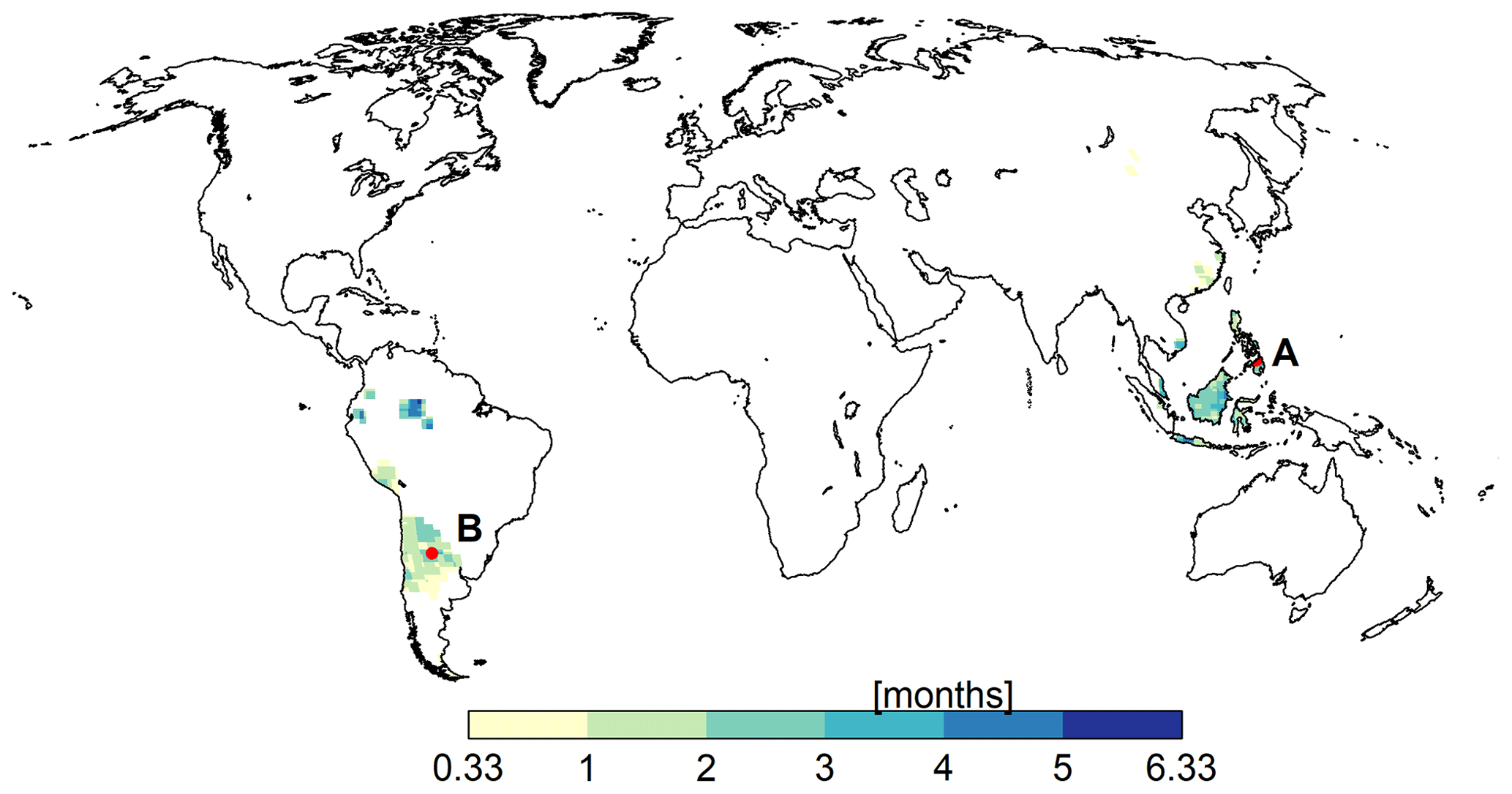
Figure 1 Mean number of calendar months per year in which evapotranspiration is in a non-water-stressed state over the reference period (1981–2000). The values shown here were obtained by averaging the output of three GCMs.

To understand the behavior of the PT-MA method at the grid cell level, two grid cells were selected: cell A (cell center at 8.75^∘ latitude, 124.75^∘ longitude) is located in the Philippines and cell B (cell center at −29.75^∘ latitude, −64.25^∘ longitude) is located in Argentina (Fig. 1). According to GFDL-ESM2M, grid cells A and B are in a non-water-stressed state for 1 and 2 months per year, respectively, during the reference period. In the case of IPSL-CM5A-LR, the corresponding values are 4 and 0 months, respectively, and in the case of HadGEM2-ES, both cells are under non-water-stressed conditions for 4 months.

2.4 A metric to quantify the impact of the PT-MA approach

We calculated a metric for quantifying the magnitude of the impact of the PT-MA approach on the change in PET and RWR with respect to the standard PT approach. The metric is a signal-to-change ratio, the relative difference of change (DC) (%):

$$\begin{array}{}\text{(5)}& {\mathrm{DC}}_{\mathrm{var}}={\displaystyle \frac{({\mathrm{dvar}}_{\text{PT-MA}}-{\mathrm{dvar}}_{\mathrm{PT}})}{{\mathrm{dvar}}_{\mathrm{PT}}}}\times \mathrm{100},\end{array}$$

where var is the variable (i.e., PET or RWR), dvar_PT-MA is the change (between future and reference periods) in the variable computed according to PT-MA approach, and dvar_PT is the change in the variable computed according to PT approach.

The DC metric can be interpreted as follows: if DC is less than −100 %, the changes as computed by the two approaches do not agree in the sign; otherwise, both approaches show either increases or decreases. PET is expected to generally increase in the future, and the increase in the case of PT-MA should be smaller than in the case of the standard PT such that negative DC values should prevail. The DC value indicates how many percent smaller the PET increase is with PT-MA compared with the standard PT. RWR, however, may increase or decrease in the future. As future RWR should generally be higher with PT-MA compared with the standard PT, due to the smaller PET change in the case of PT-MA, positive DC values should generally occur where RWR increases in the future and negative values should occur where RWR decreases. If DC is positive, the RWR increase with PT-MA is DC % larger than with PT; if DC is negative, the RWR decrease in the case of PT-MA is DC % smaller. For example, if RWR is projected to decrease by 20 mm yr⁻¹ in the case of the standard PT but by only 10 mm yr⁻¹ by PT-MA, DC = −50 %.

3 Results

3.1 Validation of the PT-MA approach

The performance of the PT-MA method is analyzed based on the area-weighted average changes in PET and R_n over non-water-stressed grid cells and months (Fig. 1), considering the changes between the reference period (1981–2000) and the future period (2080–2099) for RCP8.5, as only this RCP was considered in MD (Table 1). Table 1 also presents the respective values for the reference period. PET-PT is the PET as calculated by the standard WGHM, whereas PET-PT-MA is the result of the PT-MA method presented in Sect. 2.2. For both variants, R_n is computed based on the bias-adjusted output of the three GCMs (Sect. 2.1). PET-EO and NWSAET values for three GCMs were extracted from the MD study and are, therefore, not affected by any bias adjustment, as they had been derived by MD using the original GCM output.

The results indicate that, averaged over the three GCMs, the ensemble GCM mean PET-PT-MA change (0.31 mm d⁻¹) is only about half of the PET change computed with the standard PT (0.57 mm d⁻¹). This is similar to the reduction in the ensemble mean PET change if NWSAET or PET-EO was used instead of PET-PM for the 16 GCMs in MD. The PET-PT-MA change is much closer to the NWSAET change of 0.19 mm d⁻¹ and the PET-EO change of 0.25 mm d⁻¹ than the PET-PT change, but it still overestimates both.

For each individual GCM, PET change in the case of PT-MA is also much closer to NWSAET, PET-EO, and R_n than in the standard approach, but both PET-PT-MA and PET-EO overestimate NWSAET change (Table 1). For two of the GCMs (GFDL-ESM2M and HadGEM2-ES), PET-PT-MA and PET-EO are very similar in terms of change. However, for IPSL-CM5A-LR, PET-PT-MA overestimates the change compared with both NWSAET and PET-EO. For the three GCMs, the PT-MA method reduces the PET change by 0.18–0.31 mm d⁻¹ relative to standard PT. This is a significant reduction when compared with the range of NWSAET changes (0.10–0.27 mm d⁻¹) between the three GCMs (Table 1).

Table 1 Comparison of PET and PET changes as computed by WGHM using the standard PT and the newly developed PT-MA approach to the actual evapotranspiration computed by global climate models under non-water-stressed conditions (NWSAET) and the PET-EO approach of MD (their Figs. 1 and S2). Area-weighted averages over all non-water-stressed grid cells and months of these variables as well as of WGHM net radiation (R_n) are shown for the reference period (1981–2000). PET-PT, PET-PT-MA, and R_n are computed by WGHM using the bias-adjusted output of the listed GCMs. “Change” refers to the change between the reference period and 2080–2099 in the case of the RCP8.5 emission scenario. All values are in millimeters per day (mm d⁻¹).

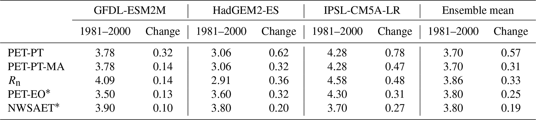
^* Milly and Dunne (2016) (MD) considered 2081–2100 to be the future period.

Differences in the PET values for the reference period, as computed with the different approaches, do not help to understand the differences in the PET changes. In the case of HadGEM2-ES, for example, where the PET-PT-MA change is larger than the NWSAET change, PET-PT-MA is much smaller than NWSAET in the reference period, while in the case of IPSL-SC5A-LR, both PET-PT-MA during the reference period and PET-PT-MA change are larger than NWSAET and its change, respectively.

The fact that changes in PET-PT-MA are very similar to changes in R_n indicates that PT-MA successfully implements the MD proposal that PET should change with R_n only in climate change impact studies (Table 1). We cannot expect perfect agreement between the changes in PET-PT-MA computed by WGHM and PET-EO computed in MD, with one reason being that the spatial and temporal resolutions are different. Possibly more important are the differences in the R_n computation. R_n of WGHM depends not only on the downward shortwave and longwave radiation provided by the GCMs but also on the WGHM estimation of upward shortwave and longwave radiation. In addition, the climate input for PET-PT-MA is bias-adjusted GCM output, whereas there was no bias adjustment for PET-EO. When comparing R_n change with PET-EO change, which is computed as the change in 0.8R_n, it can be concluded that R_n change is likely higher (GFDL-ESM2M and HadGEM2-ES) or lower (IPSL-CM5A-LR) in the original GCMs than in the WGHM, where R_n is computed from bias-adjusted GCM output (Table 1).

The temporal development of the two PET variants and R_n between 1901 and 2099 for the non-water-stressed cells and months, as computed by WGHM, does not show, for all three GCMs, appreciable trends in the 20th century for PET or R_n (Fig. 2a, c, e). In the 21st century, the variables increase strongly. Reflecting the PT-MA method (Sect. 2.2), PET-PT and PET-PT-MA only start to deviate from each other after the end of the selected reference period (here 1981–2000) of the climate change study. PET-PT-MA increases less strongly after 2000 than PET-PT and is very similar to R_n. By the end of the 21st century, the 9 %–19 % PET increase projected for the NWSAET cells and months by the standard PT method for the three GCMs is reduced to 4 %–11 % if PT-MA is applied (compared with the start of the 21st century). Based on Koster and Mahanama (2012), MD proposed, with PET-EO, that climate-change-driven PET change is not equal to the R_n change but to only 80 % of the R_n change. The slopes of the PET-PT to R_n regression lines are much larger than 0.8, ranging from 1.42 to 1.73, while the values for PET-PT-MA are reduced to 0.9–1.02 (see Fig. 2b, d, f). Thus, according to the PT-MA approach implemented in WaterGAP, a larger fraction of the additional net radiation evaporates under non-water-stressed conditions than assumed by MD. This may be explained by the selection of grid cells with a relatively high mean temperature (see Fig. 1). While a slope of 0.80 results from a temperature value of 16 ^∘C in the case of α=1.26 according to Eq. (1), slopes of 0.9 and 1.02 result from temperature values of 22 and 33 ^∘C, respectively. The interannual variability in the PET time series closely follows the variability in the R_n time series (Fig. 2a, c, e).

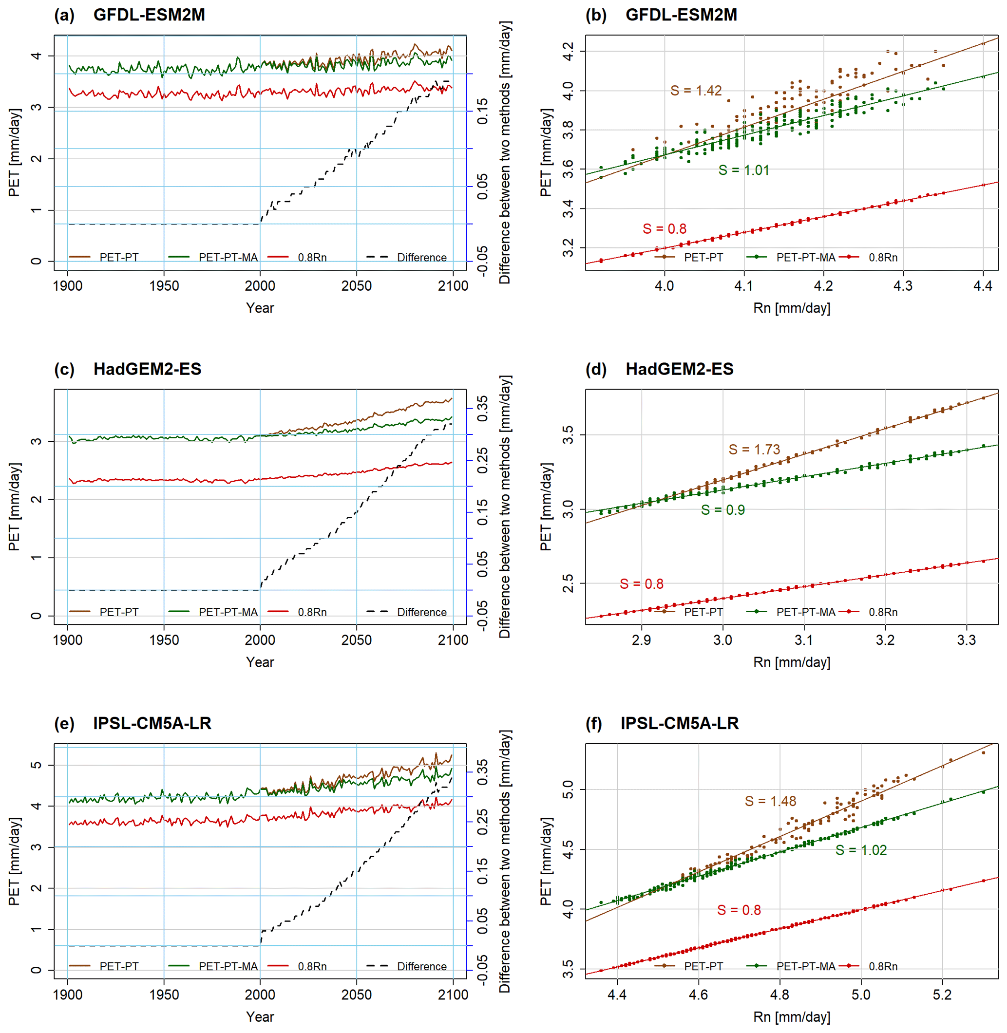
Figure 2 Area-weighted average over non-water-stressed grid cells and months of PET-PT (brown), PET-PT-MA (green), and 0.8R_n (red) for all years of 1901–2099 computed based on daily WGHM output, forced by GCM bias-adjusted climate data under RCP8.5. Time series plots are given in panels (a), (c), and (e). Scatterplots between R_n and two PET schemes are presented in panels (b), (d), and (f). In the time series plots, the difference between PET-PT and PET-PT-MA (“Difference”) is given on the secondary y axis (dashed black line). Please note that different grid cells and months are aggregated for each GCM. “S” is the slope of the trend line.

3.2 Temporal development of PET at two locations

At the selected locations A and B (see Fig. 1), PET is projected to increase in the future except for location A in the case of the GFDL-ESM2M climate model (Figs. 3, B1). With GFDL-ESM2M climate input, a slightly decreasing trend in both PET-PT and, more so, PET-PT-MA is observed at location A (as well as in very small areas elsewhere), corresponding to the relatively small temperature increase computed by this GCM for location A and globally (see Fig. B1c).

When comparing the two time series of PET-PT and PET-PT-MA until 2001, there is no difference between the two methods, as intended. From 2001 onwards, the rate of PET increase with the PT-MA method is smaller than with the standard PT method. As a result, the difference between PT and PT-MA is increasing over time and varies among the GCMs and locations (dashed black line in Fig. 3a, b, e, and f). Removal of the long-term temperature trend (Sect. 2.2) is successfully done in the PT-MA method (compare Figs. S1–S4 in Supplement). Both T_modified and PT-MA to R_n ratios do not show a trend in cells A and B in the 21st century, but a GCM-specific interannual variability is still observed (see Fig. 3c, d, g, h).

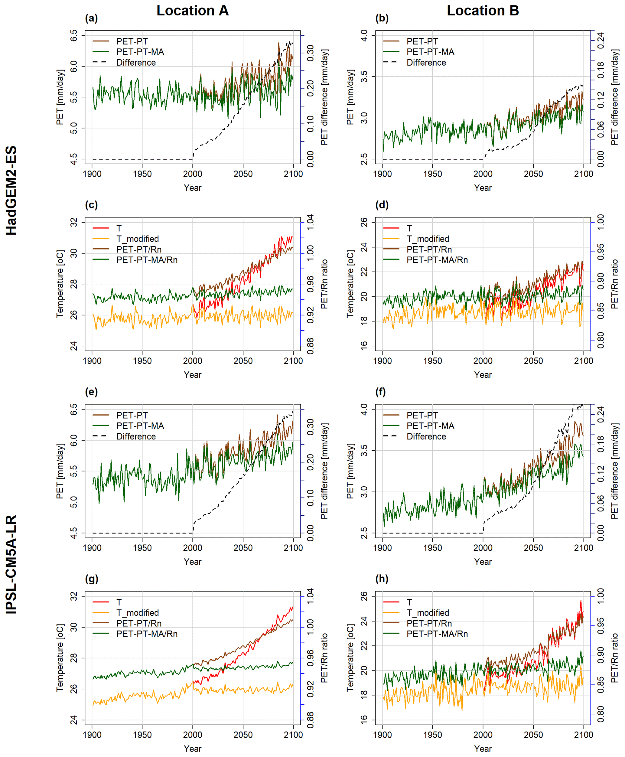
Figure 3 Annual time series of PET and temperature at location A (a, c, e, g) and location B (b, d, f, h), as computed by the WGHM forced by HadGEM2-ES (a–d) and IPSL-CM5A-LR (e–h) under the RCP8.5 scenario. In panels (a), (b), (e), and (f), PET with PT (brown) and PET with PT-MA (green) are shown on the primary y axis. The difference between the two methods (dashed black line) is given on the secondary y axis. In panels (c), (d), (g), and (h), the PET to R_n ratio for the PT method (brown) and PT-MA (green) method are on the secondary y axis and the bias-adjusted input temperature (red) and modified temperature (yellow) are on the primary y axis.

3.3 Spatially heterogeneous future mean PET changes

We compared the projected future absolute changes in mean annual net radiation, standard Priestley–Taylor PET-PT and the modified PET-PT-MA (Figs. 4a–f, B2a–f). Hereafter, in the main text, we present the results corresponding to only two GCMs, while the results for the other two GCMs are shown in the Appendix.

Change refers to the difference between the 2080–2099 period and the reference period (1981–2000) under RCP8.5. According to the HadGEM2-ES and IPSL-CM5A-LR GCMs, net radiation increases in the future, with the IPSL-CM5A-LR model projecting a stronger increase. The spatial patterns of change in PET-PT-MA (dPET-PT-MA) are very similar to those of net radiation change (dR_n), as is intended by the PT-MA approach to compute PET. Increases in PET-PT are much higher than increases in PET-PT-MA. dPET-PT values for the HadGEM2-ES climate model, which has smaller dR_n values than the IPSL-CM5A-LR model, are even higher than dPET-PT-MA values for the IPSL-CM5A-LR model.

The Wilcoxon signed-rank test for paired samples was applied to understand the significance of the differences between the time series of annual PET for 2080–2099 as computed by either the standard PT or the modified PT-MA approach. The null hypothesis is “The median difference between the values computed by two methods is zero (i.e., no significant difference)”; it is rejected at a 95 % level of significance. For all GCMs, it was found that there is a significant difference between the PET values computed by the two alternative approaches in all grid cells.

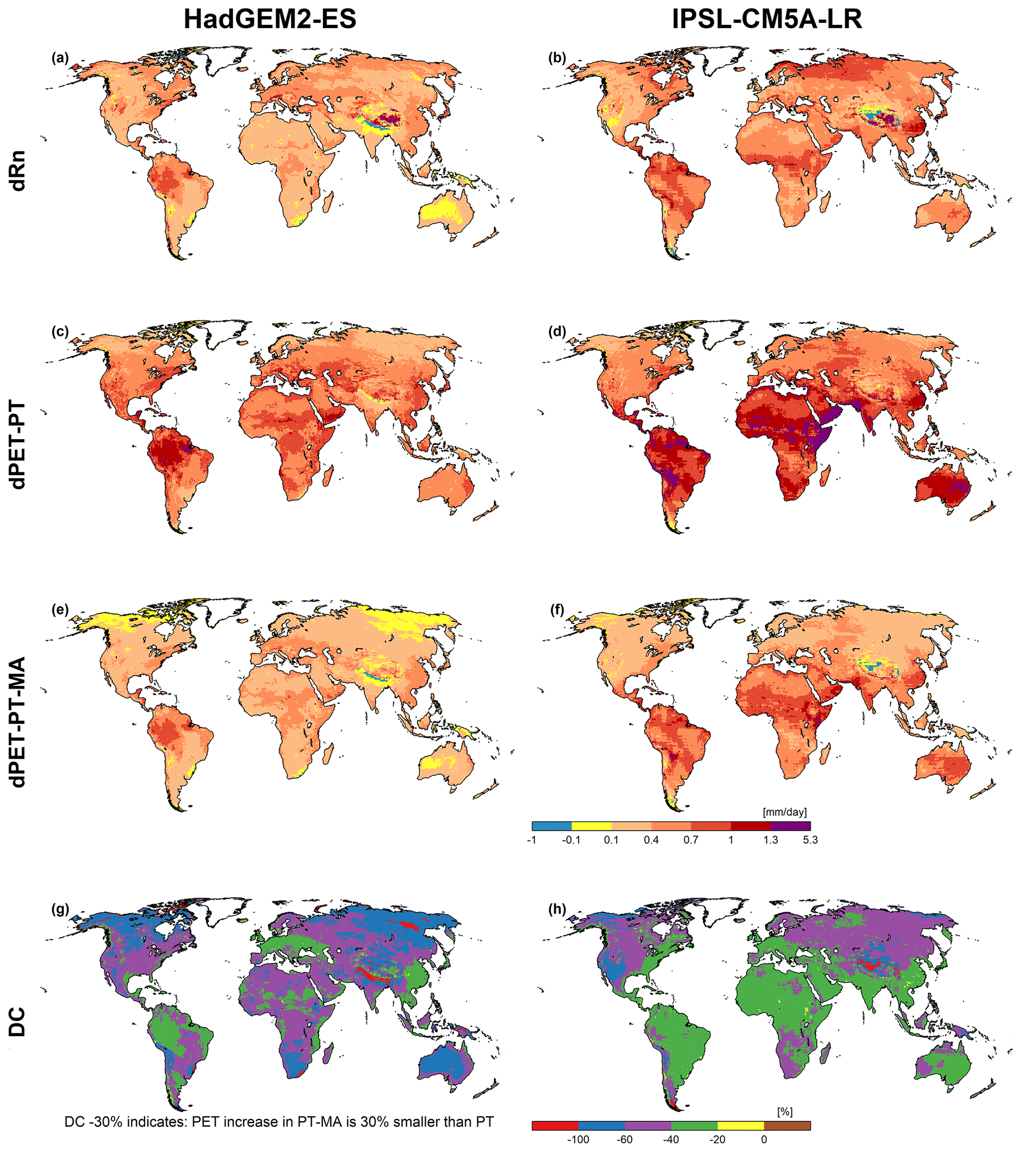
Figure 4 Net radiation (R_n) and PET changes computed by WGHM forced with HadGEM2-ES (a, c, e, g) and IPSL-CM5A-LR (b, d, f, h) climate data between the reference (1981–2000) and the future (2080–2099) period under RCP8.5. Panels (a) and (b) show the average R_n change (dR_n), panels (c) and (d) present the average PET change with PT (dPET-PT), panels (e) and (f) show the average PET change with PT-MA (dPET-PT-MA), and panels (g) and (h) present the percent difference of dPET-PT-MA and dPET-PT (DC). A DC value of, e.g., −50 % indicates that PET-PT-MA increases only half as much as PET-PT.

The relative difference of change, DC ((dPET-PT-MA-dPET-PT)/dPET-PT), is, as expected, negative almost everywhere and differs between the GCMs (see panels g and h of Figs. 4 and B2). As explained in Sect. 2.4, the more negative the DC values are, the more the PET increase computed by PT is reduced in the case of PT-MA relative to dPET-PT. Relative reductions in the PET increase are larger for the HadGEM2-ES GCM than for the IPSL-CM5A-LR GCM, likely due to the lower absolute increases in PET-PT. In some parts of Australia, for example, the new PET approach leads to a reduction in the PET increase of more than 60 % and 20 %–40 % in the case of HadGEM2-ES and IPSL-CM5A-LR, respectively. In the few red grid cells (which indicate that DC is less than −100 %), PET-PT increases while PET-PT-MA decreases. There are very few grid cells projecting a decrease (brown areas) in the average PET for both methods (compare panels g and f of Figs. 4 and B2).

3.4 Spatially heterogeneous future mean changes in renewable water resources

While a reduction in the projected PET increase due to the new PT-MA method is expected to lead to higher projected runoff and, thus, higher renewable water resources (RWR) values compared with the standard approach, the relative increase depends on how much AET is limited by water availability in the soil and open water bodies and, thus, also depends on changes in precipitation. If a large part of a grid cell consists of open water bodies, the RWR increase will be small, as the PET of open water is not affected by the PT-MA method. In addition, higher runoff and, thus, upstream streamflow may lead to increased AET and, thus, decreased RWR in downstream grid cells due to evaporation from surface water bodies or irrigated fields. Therefore, the effect of the alternative PT-MA approach to compute PET on AET and, subsequently, RWR is more intricate than its effect solely on PET.

Changes in precipitation (dP) as projected by GCMs, with different global patterns (Fig. 5a, b), are the main drivers of changes in RWR (dRWR). Increasing P will mostly result in RWR increases unless the P increase is small such that increased AET leads to decreased RWR (Fig. 5c, d, e, f). For instance, when comparing Fig. 5a and c, precipitation slightly increases in grid cells in the Prairie Provinces of Canada but RWR slightly decreases.

To assess the significance of the differences between the RWR values computed with the PT and the PT-MA variants at the grid cell level, we employed the Wilcoxon signed-rank test for the time series of annual RWR from 2080 to 2099, similar to the approach used for the PET analysis (Sect. 3.3). For 0.5^∘ grid cells shown in light gray in Figs. 5g and h and B3e, f, g, and h, differences resulting from the two alternative variants are insignificant.

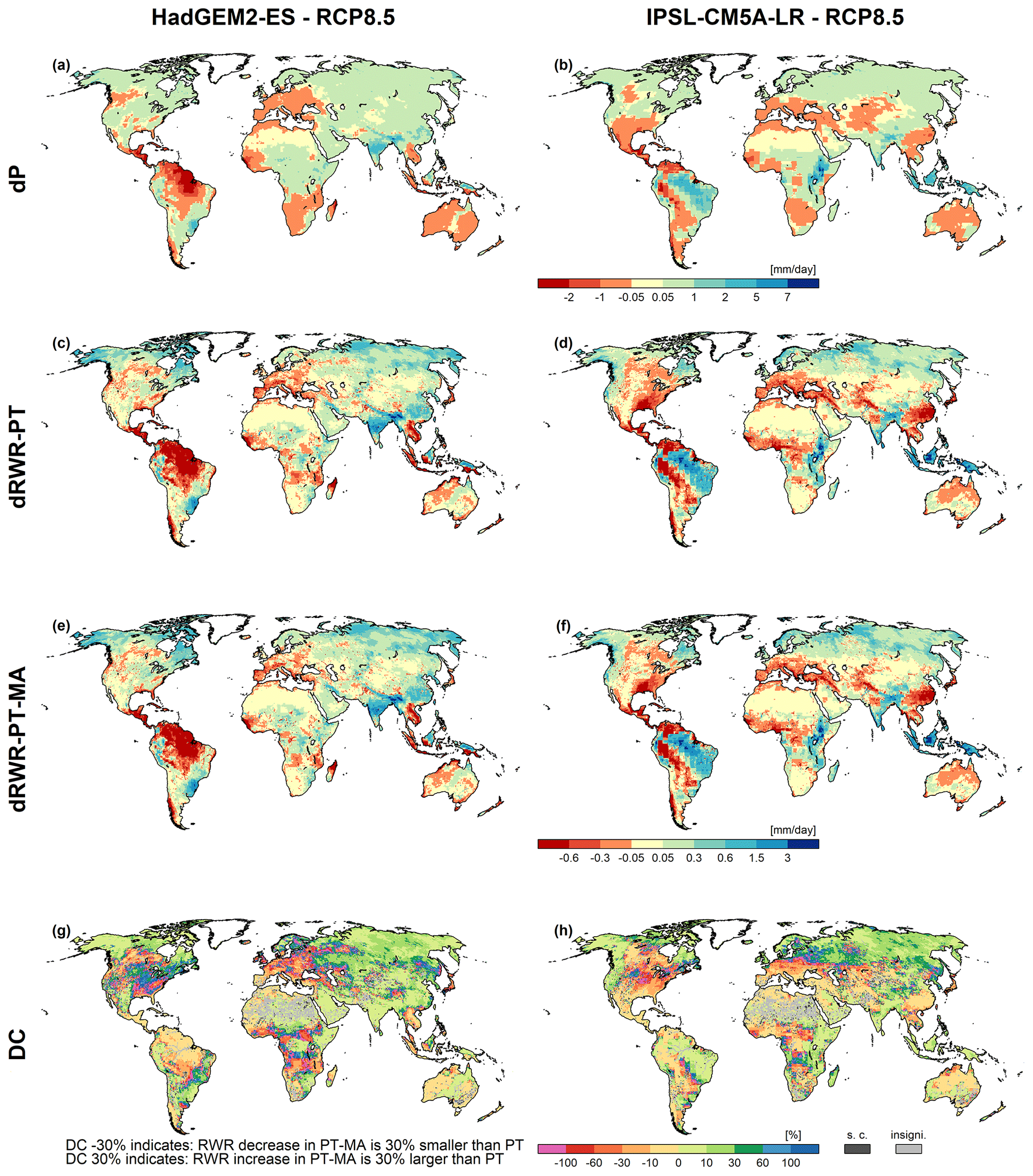
Figure 5 Precipitation (P) and renewable water resources (RWR) changes for HadGEM2-ES (a, c, e, g) and IPSL-CM5A-LR (b, d, f, h) climate data between the reference (1981–2000) and the future (2080–2099) period under RCP8.5. Panels (a) and (b) show the absolute change in average precipitation between future and reference periods (dP), panels (c) and (d) present the absolute change in average RWR computed with the PT method (dRWR-PT), panels (e) and (f) show the absolute change in average RWR computed with the PT-MA method (dRWR-PT-MA), and panels (g) and (h) show the percent difference of dRWR-PT-MA and dRWR-PT (DC). Cells where dRWR-PT-MA < dRWR-PT are denoted as special cases (“s.c.”). The cells labeled as “insigni.” represent instances where the computed change in RWR using the two methods is not statistically significant. As the difference is positive in all other cells, a negative DC value indicates a future decrease in RWR-PT, whereas a positive DC value indicates a future increase.

The spatial patterns of future increases and decreases in dRWR-PT and dRWR-PT-MA appear to be very similar (Fig. 5c, d, e, f), and the expected higher future RWR-PT-MA, with dRWR-PT-MA > dRWR-PT, i.e., higher RWR increases and lower RWR decreases, is not well visible. This is due to both the strong impact of dP on dRWR and the strong spatial variability in the projected increases and decreases. Stronger RWR decreases by the PT approach compared with the PT-MA approach are only visible from, e.g., the slightly larger red areas in Africa and South America for the IPSL-CM5A-LR GCM. The DC metric (Fig. 5g, h) directly quantifies the differences in the future change in RWR between the two PET variants. Negative DC values indicate areas with future decreases in RWR-PT, where the standard PET approach overestimates drying compared with the modified approach. Positive values indicate areas with future increases in RWR-PT, where the standard method underestimates the increases compared with the modified approach. For example, the RWR decrease in Central America and the downstream Amazon in the case of HadGEM2-ES is less than 10 % smaller in the case of computing PET-PT-MA than in the standard approach (yellow color), while it is up to 30 % less in the upstream Amazon and in parts of central and western Europe (orange color). Higher values of up to 100 % are computed for areas scattered around the world, for all four investigated GCMs (compare Fig. 5g and h and Fig. B3e and f). Green to blue indicates areas where the standard approach underestimates the future increase in RWR. As in the case of decreases, differences of less than 10 % dominate but higher discrepancies of up to 30 % occur in large areas of Siberia. They can exceed even 100 % where projected increases are small. The pink color identifies grid cells where the RWR slightly decreases in the case of the standard approach but slightly increases in the case of PT-MA.

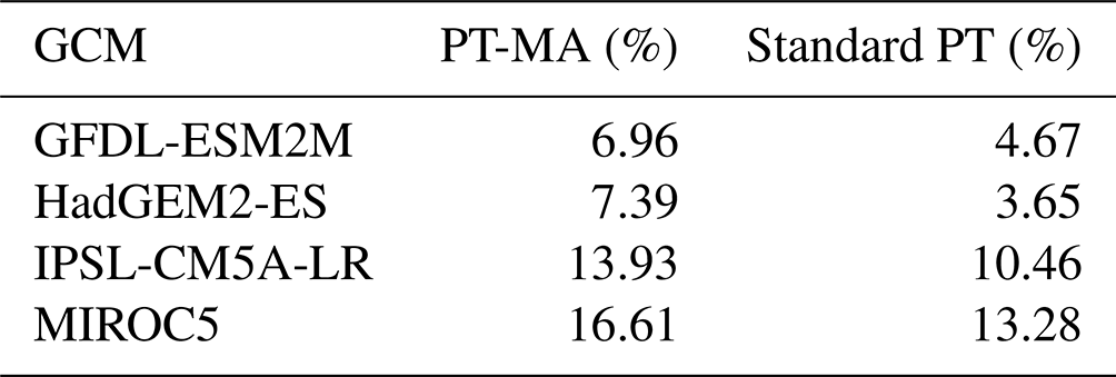
In a small number of grid cells, 3 % in the case of HadGEM2-ES and 4 % in the case of IPSL-CM5A-LR, dRWR-PT-MA is smaller than dRWR-PT. These special cases can be explained by the lateral flow processes in combination with lakes and wetland and/or irrigation that are represented in WaterGAP but not in GCMs. RWR in WaterGAP represents the net amount of liquid water that is added or removed per time step by the processes within a grid cell, averaged over the analysis period. It is computed as the difference between the streamflow leaving the cell and the streamflow entering the cell. In most grid cells, outflow is larger than inflow, and the positive RWR reflects the part of the precipitation on the land and the surface water bodies of the grid cell that does not evapotranspire. In the case of lakes and wetlands that are recharged by upstream streamflow as well as in the case of irrigation, outflow from the cell may become smaller than inflow; thus, RWR is negative. Cells where PT-MA does not lead to higher RWR compared with PT are mainly cells with lakes and wetlands (including internal sink cells) that receive inflow from upstream cells (e.g., wetlands along the Amazon or the Niger rivers) or cells with a high irrigation water use. In the case of PT-MA, cells with such lakes or wetlands receive a higher inflow from upstream, which leads to an increased surface water area and, thus, increased evaporation from the surface water body. Therefore, even if the grid cell runoff from soil increases in the case of PT-MA, the increased evaporation from the surface water body can dominate and lead to a decreased RWR of the grid cell. The same can happen in grid cells with large irrigation water demand from surface water bodies that can be fulfilled better in the case of increased streamflow, leading to increased evapotranspiration in the cell and, thus, possibly lower RWR. Note that, to calculate PET from surface water bodies or irrigation water demand, PET is computed according to the standard PT approach. The PT-MA approach to compute PET change increases total globally averaged RWR more strongly than the standard PT approach, for all four GCMs (Table 2). However, while the increase in RWR is more than 100 % larger for HadGEM2-ES, it is only 50 % larger for GFDL-ESM2M and even less for the other two GCMs.

Table 2 Projected change (%) in renewable water resources between 1981–2000 and 2080–2099 for the RCP 8.5 emission scenario in the case of computing PET with the modified (PT-MA) and the standard (PT) approach, averaged over the global land area (excluding Antarctica and Greenland).

3.5 Analyses for other RCPs

MD analyzed only GCM simulations that implemented the RCP8.5 high-emission scenario. As for individual GCMs, increases in CO₂ concentrations and temperature are roughly correlated (Humlum et al., 2013). We also applied the PT-MA approach for other RCPs. In RCP2.6, projected precipitation changes are smaller than under RCP8.5 (compare Fig. 6a and b with Fig. 5a and b). For each GCM, spatial DC patterns for RWR under RCP2.6 are rather similar to those under RCP8.5 (compare Fig. 6c and d with Fig. 5g and h). Under RCP2.6, the differences between dRWR computed by the two approaches are only slightly smaller than under RCP8.5 (Fig. 7b).

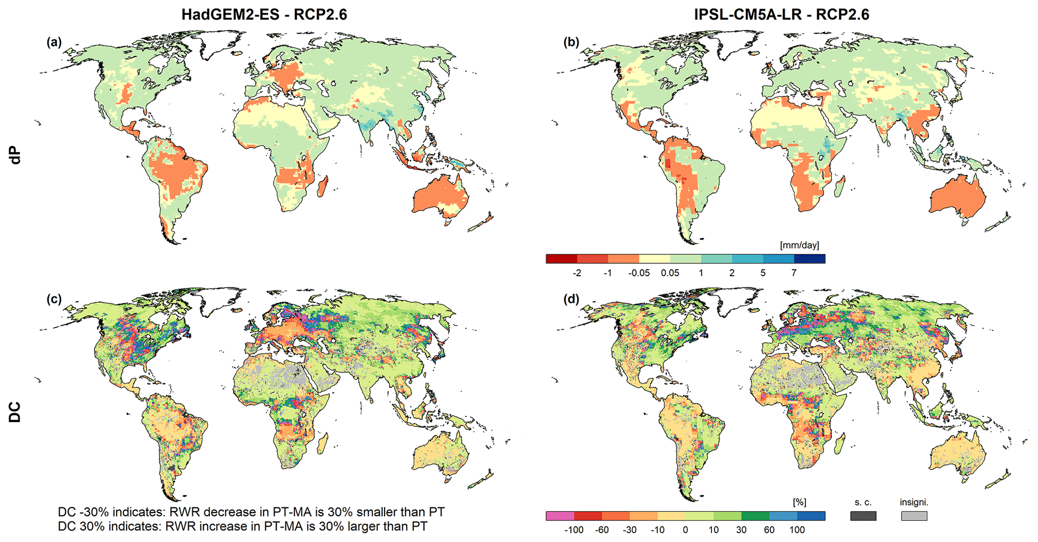
Figure 6 Projected RWR changes for HadGEM2-ES (a, c) and IPSL-CM5A-LR (b, d) climate data between the reference (1981–2000) and the future (2080–2099) period under RCP2.6. Panels (a) and (b) show the absolute change in average precipitation (dP) and panels (c) and (d) present the percent difference in dRWR-PT-MA and dRWR-PT (DC). Cells where dRWR-PT-MA < dRWR-PT are denoted as special cases (“s.c.”). The cells labeled as “insigni.” represent instances where the computed change in RWR using the two methods is not statistically significant.

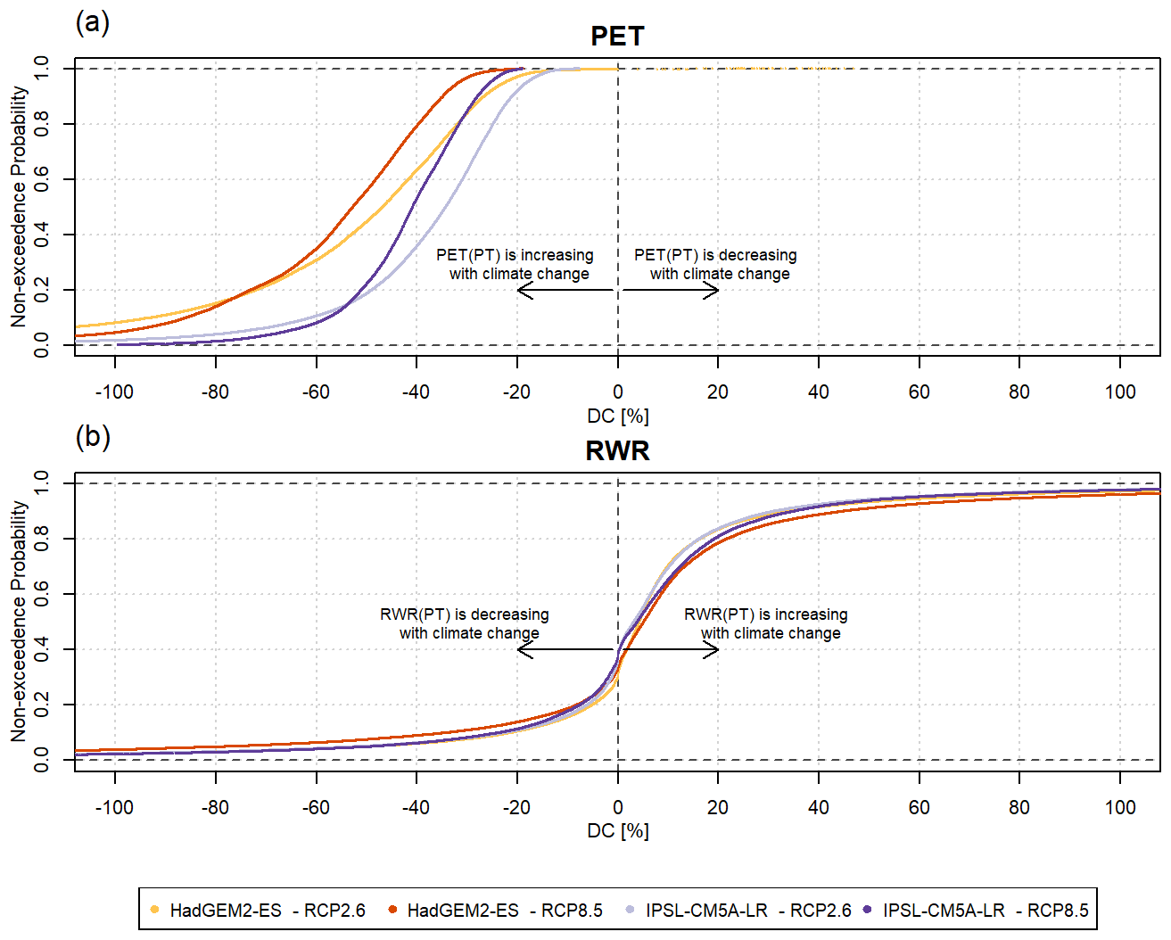
Figure 7 The cumulative probability distributions of DC, i.e., the relative difference between the change computed with the PT-MA approach and the change computed with the standard PT method for (a) PET and (b) RWR. The results are based on WGHM output forced with HadGEM2-ES and IPSL-CM5A-LR climate models under RCP8.5 and RCP2.6. The lighter colors correspond to RCP2.6 and the darker colors correspond to RCP8.5. Antarctica and Greenland are excluded.

Global DC-RWR distributions for the two GCMs are similar, while HadGEM2-ES leads to a slightly higher impact of PT-MA than IPSL-CM5A-LR (Fig. 7b). Regardless of the RCP or the GCM, most grid cells have a DC of between −10 % and 20 %. About 60 % of the DC values are positive, indicating that about 60 % of all grid cells also indicate an increase in RWR with both the PT and PT-MA methods in the future period compared with the historical period.

In contrast to DC-RWR, the cumulative probability distributions of DC-PET differ appreciably between RCP8.5 and RCP2.6 and between the GCMs (Fig. 7a). The reduction in the PET increase in the PT-MA approach compared with the standard PT method is smaller in the case of RCP2.6. Reductions are larger for HadGEM2-ES (−60 % to −30 % under RCP8.5) than for IPSL-CM5A-LR (−50 % to −20 %), likely due to the higher temperature increase in the Northern Hemisphere and, thus, the stronger temperature reduction in the case of HadGEM2-ES (see Fig. A1).

Averaged globally and over all four GCMs, the three land water balance components, precipitation, AET, and streamflow into oceans and internal sinks (i.e., RWR), are projected to increase in the future due to climate change, with increases becoming greater with greenhouse gas emission rises (Fig. 8). This is also the case for PET. With the proposed PT-MA approach, global-scale PET increases of 6.9 %–18.9 % (four RCPs) for the standard approach are strongly decreased to 4.4 %–10.7 %. The effects of PT-MA on global changes in AET and RWR are of similar magnitude. While AET increases of 3.1 %–5.7 % are decreased to 2.4 %–3.7 % (Fig. 8c), RWR increases of 1.6 %–8.0 % are increased to 2.8 %–11.2 % (Fig. 8c).

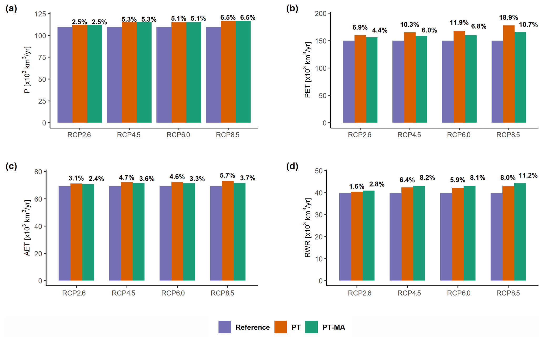
Figure 8 Effect of the PT-MA and the standard PT approach to compute PET on the water balance of the global land area. Ensemble mean across the four GCMs of globally aggregated (a) precipitation (P), (b) potential evapotranspiration (PET), (c) actual evapotranspiration (AET), and (d) streamflow into oceans and inland sinks (renewable water resources – RWR) according to WGHM for the periods 1981–2000 and 2080–2099. The percentage values at the top of the bars indicate the relative change in the variable compared with the reference period value. Antarctica and Greenland are excluded.

4 Discussion

4.1 Sources of uncertainty in the projected PET change

To understand the magnitude of the uncertainty in PET changes related to the choice of PET approach (PT-MA or PT), we compared it to the magnitude of the uncertainty related to the choice of GCM. The computed absolute change in PET between the periods 1981–2000 and 2080–2099 computed by WGHM that was forced by four GCMs under the RCP8.5 scenario is used in this uncertainty analysis. The uncertainty range that stems from the four GCMs (GCM_range) is computed as follows:

$$\begin{array}{}\text{(6)}& {\mathrm{GCM}}_{\mathrm{range}}={\displaystyle \frac{\begin{array}{c}{\sum }_{m=\mathrm{1}}^{\mathrm{2}}|\mathrm{\Delta }{\mathrm{PET}}_{{\mathrm{GCM}}_{(m,\text{highest out of four GCMs})}}\\ -\mathrm{\Delta }{\mathrm{PET}}_{{\mathrm{GCM}}_{(m,\text{lowest out of four GCMs})}}|\end{array}}{\mathrm{2}}},\end{array}$$

where m=1–2 corresponds to the two PET estimation methods (PT-MA and PT).

The uncertainty that originates from the two different PET computation approaches (Approach_range) is calculated as follows:

$$\begin{array}{}\text{(7)}& {\mathrm{Approach}}_{\mathrm{range}}={\displaystyle \frac{\begin{array}{c}{\sum }_{n=\mathrm{1}}^{\mathrm{4}}|\mathrm{\Delta }{\mathrm{PET}}_{{\mathrm{GCM}}_{(n,\text{PET-PT-MA})}}\\ -\mathrm{\Delta }{\mathrm{PET}}_{{\mathrm{GCM}}_{(n,\text{PET-PT})}}|\end{array}}{\mathrm{4}}},\end{array}$$

where n=1–4 corresponds to the four GCMs applied in this study.

Figure 9 shows the GCM uncertainty and the approach uncertainty as percentages of the total uncertainty, i.e., the sum of GCM_range and Approach_range. In most regions, GCM uncertainty is the dominant source of uncertainty. On global average, the choice of GCM is responsible for 62 % of the total uncertainty. The PET approach uncertainty is dominant in large parts of North America, Central Asia, and Africa. In most regions of the globe, the PET approach causes at least 30 % of the total uncertainty. The minimum contribution of GCM uncertainty is 16 %, while the minimum contribution of the PET approach is 0 %, due to grid cells that only consist of open water. This analysis shows that the choice of the PET approach has a significant impact on the computed PET change when compared with the impact of the well-known large uncertainty in climate projections that is caused by applying different climate models.

Using an ensemble of model output derived from two variants of PET calculation methods is crucial for capturing the full range of uncertainty associated with vegetation response in climate change impact assessment studies.

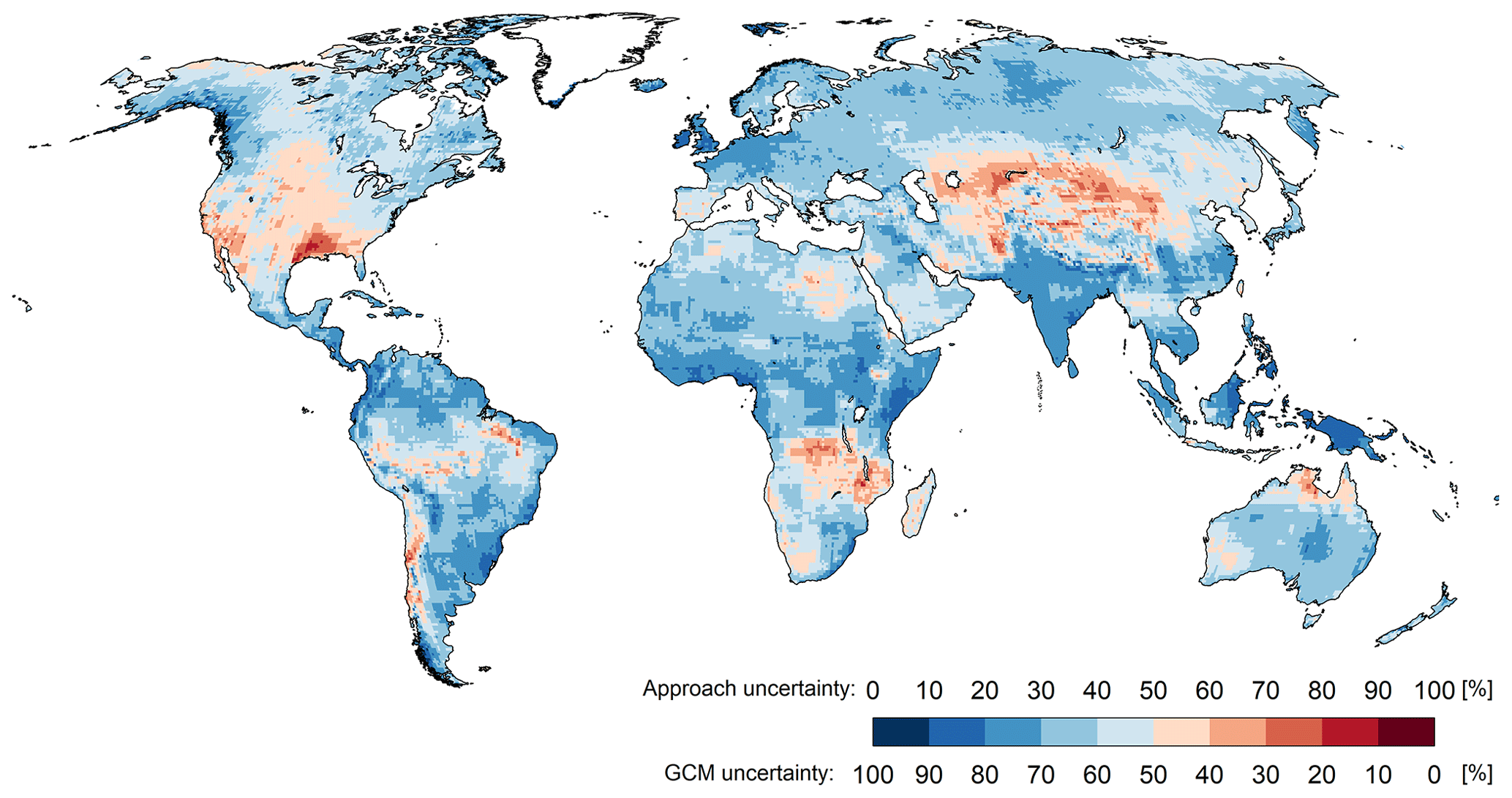
Figure 9 Source of uncertainty in the projected PET change based on WGHM output that is derived from two PET calculation approaches and four GCMs under the RCP8.5 scenario.

4.2 Caveats and applicability

This paper presents a method that enables hydrological models that compute PET as a function of net radiation and temperature to simulate future PET such that PET changes with net radiation only. The estimation of PET changes by the PT-MA approach is obviously also affected by uncertainties in the estimation of net radiation changes. In our study, the latter were computed from changes in downward shortwave and longwave radiation as provided by GCMs and changes in upward shortwave and longwave radiation as computed by WGHM.

The concept that PET change under climate change can be approximated by the change in net radiation was derived by MD, who analyzed changes in actual evapotranspiration as computed by a number of GCMs for only a small number of grid cells and months in tropical climates that do not experience water stress. This means that our approach assumes that vegetation response to climate change around the globe is similar to that of tropical vegetation under a given change in net radiation and temperature. Such a spatially homogeneous response cannot be expected. In particular, in the PT-MA approach, PET is always less than that computed using the standard PT approach. While different DGVMs tend to simulate this behavior for many regions, the total balancing of the warming effects seen in the non-water-stressed tropical grid cells of the GCMs might not be true for other biomes. How much, if at all, the physiological effect (closure of stomata) dominates over other effects such as the structural effect (increase in biomass/leaf area) and biome shifts in a certain biome, is, however, not well known. Different from the PET change computed with PT-MA, DGVMs predict a spatially heterogeneous vegetation response to climate change, which leads to a relative increase in PET in some regions. Unfortunately, there are considerable differences between the simulation results of different DGVMs, and there is no agreement on where the vegetation response leads to increased or decreased PET (Reinecke et al., 2021).

Therefore, we propose that two alternative model variants are routinely used in climate change impact studies with hydrological models that do not simulate vegetation processes: in one variant, the standard PT approach is selected to compute the PET of the vegetated land surface, whereas the PET-MA approach is selected in the other variant. In this way, the uncertainty in PET due to the vegetation response can be taken into account. The disadvantage is that the number of model runs is doubled, as the two variants need to be run for each alternative GCM or RCP that determines the model input. While application of only the standard PET approach has been shown to overestimate future drying, i.e., overestimate the decrease in water resources, or underestimate the increase in future water resources (Milly and Dunne, 2016; Yang et al., 2019), application of the newly proposed PT-MA might overestimate the impact of stomatal closure due to increasing atmospheric CO₂ concentrations in some regions, and PET estimation with the standard PT approach is more appropriate, as indicated by the studies of Milly and Dunne (2017) and Reinecke et al. (2021). Therefore, without further knowledge on the local vegetation-specific response to climate change, it is best to simulate hydrological changes under climate change with an ensemble approach, i.e., running the model with both PET variants.

The PT-MA approach can be used if PET is calculated as a function of net radiation and temperature only, as in the PT equation. To our knowledge, the PT equation is the sole PET equation that computes PET as a function of temperature and net radiation only. If a hydrological model uses a Penman–Monteith-type equation to estimate PET, the approach of Yang et al. (2019), where stomatal conductance is adjusted, is suitable to compute PET changes under climate change. However, the application of the Penman–Monteith-type equation demands more input data than the PT equation, requiring data on humidity and wind speed, which is why many local and regional models do not use this type of PET equation (Lu et al., 2005; Koedyk and Kingston, 2016). Furthermore, if hydrological models use a Penman–Monteith-type equation, assessment of climate change impacts requires downscaled humidity and wind speed projections, which are quite uncertain (Randall et al., 2007). This limits the usability of Penman–Monteith-type equations.

Therefore, the use of the PT equation is a good option for simulating PET in hydrological models, and these models can then implement the PT-MA approach to compute scenarios of future hydrological hazards due to climate change. Widely used basin-scale hydrological models, such as HBV/HBV-Light or SWAT, are well suited for applying the PT-MA approach, as they use daily PET time series as input that can be computed using the PT equation (Rajib et al., 2018; Koedyk and Kingston, 2016). The user can pre-compute time series of daily PET for the study area using the PT-MA approach and then use them as a model input. Other radiation-based PET equations, such as Jensen–Haise, Makkink, and Turc, that do not consider net radiation but rather components of net radiation, such as shortwave radiation, should not be used for climate change studies (if the hydrological model does not simulate the interactions between the atmosphere and land surface), and these methods should not be adapted according to the proposed approach.

5 Conclusions

Application of standard equations for estimating PET in hydrological models, such as the Penman–Monteith or Priestley–Taylor-type equations, was shown to lead to an overestimation of future PET for many regions of the globe, mainly due to neglecting the impact of vegetation responses to changing atmospheric CO₂ concentrations and climate. As a result, future decreases in renewable water resources may be overestimated or future increases may be underestimated. With the proposed method for PET computation in hydrological models that do not simulate vegetation processes, future PET changes occur only in response to changes in net radiation. This was shown by MD to be consistent with the changes in non-water-stressed AET computed by a number of GCMs, which simulate the complex interaction between soil, vegetation, and the atmosphere, including the vegetation response to changing atmospheric CO₂ concentrations and climate. However, at least in some regions, although these cannot be defined with certainty, the vegetation response is such that standard PET computation leads to more reliable results. To take the uncertainty in future PET changes due to the vegetation response into account, we propose that climate change impact studies by hydrological models should always include runs with two model variants: one with the standard PET approach and the other with a modified approach. The two variants, which approximately represent the uncertainty bounds related to the vegetation response to climate change, improve the estimation of the total uncertainty in future hydrological changes.

The modified approach to compute Priestley–Taylor PET under climate change, PT-MA, is suitable if PET is computed according to the Priestley–Taylor equation, whereas the approach of Yang et al. (2019) should be applied if one of the more data-intensive Penman–Monteith-type equations can be used in the hydrological model. In the latter case, we propose checking whether the thus computed change in PET is approximately equal to the change in net energy input to the land surface. Implementation of the PT-MA approach is very simple, and the reference period for the climate change study can be easily adjusted.

When implementing the PT-MA approach in the global hydrological model WaterGAP 2.2d, the projected increase in global renewable water resources and streamflow into oceans is enhanced. The PT-MA approach leads to reduced drying (smaller decrease in renewable water resources) or increased wetting (stronger increase in renewable water resources) compared with the standard Priestley–Taylor equation for almost all grid cells, for both RCP2.6 and RCP8.5. Only in a few cells (3 %–4 %) does consideration of the vegetation response lead to lower renewable water resources compared with the standard approach; these are grid cells in which increased lateral inflow leads to an increased extent of surface water bodies and, thus, evapotranspiration or in which large irrigation demands can be fulfilled better by increased streamflow.

Regarding future research, we propose a global-scale comparison of changes in PET and renewable water resources as computed by WaterGAP using the PT-MA approach to changes computed by various DGVMs (or land surface models that simulate the vegetation response), in order to better understand the climates and vegetation types for which the PT-MA approach is too simplistic and cannot capture, for example, that the vegetation response leads to an increase in PET. In addition, we propose comparing PT-MA-derived PET projections to those obtained by applying the Yang et al. (2019) approach to Penman–Monteith-type equations, in order to determine whether both approaches lead to similar PET changes for any given GCM climate scenario.

Appendix A: Temperature reduction factor

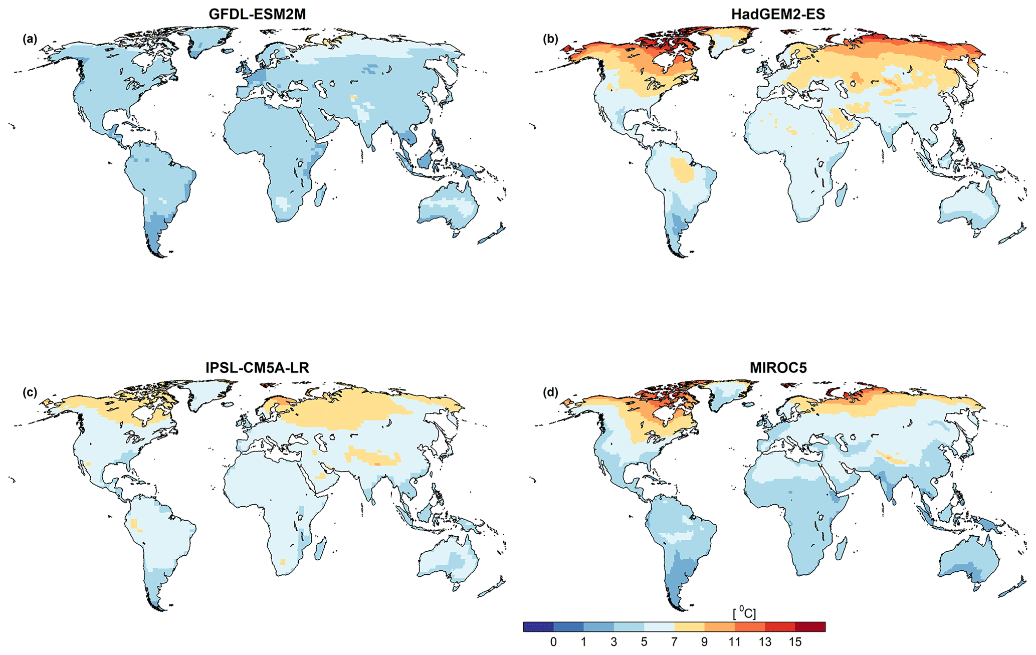
Figure A1 Spatial distribution of the temperature reduction factor for the year 2089.

Appendix B: Additional results

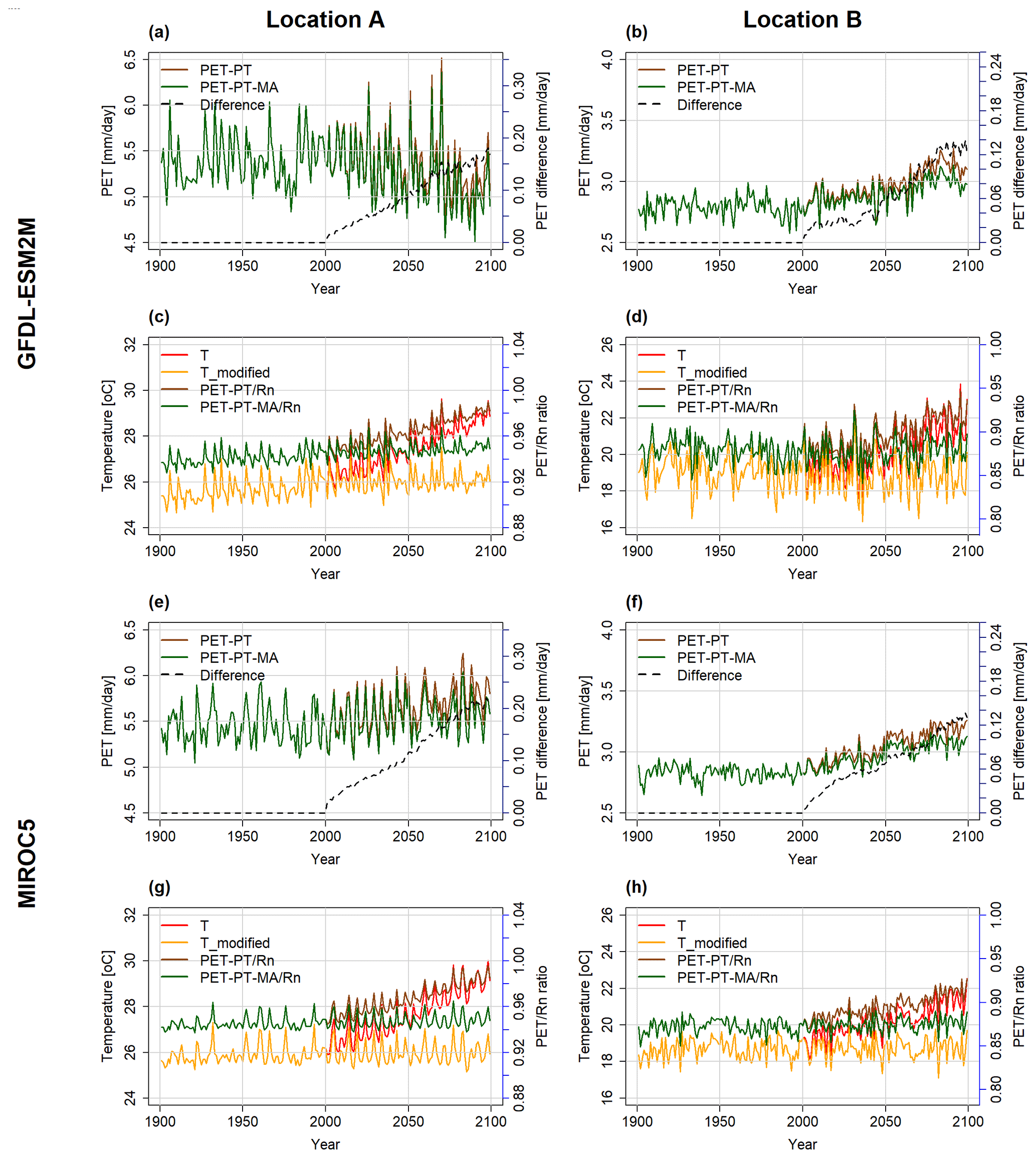
Figure B1 Temporal development of the PET and temperature variables at location A (a, c, e, g) and location B (b, d, f, h), as computed by the WGHM forced by GFDL-ESM2M (a–d) and MIROC5 (e–h) under the RCP8.5 scenario. In panels (a), (b), (e), and (f), PET with PT (brown) and PET with PT-MA (green) are on the primary y axis and the difference between the two methods (dashed black line) is on the secondary y axis. In panels (c), (d), (g), and (h), the PET to R_n ratio with the PT method (brown) and PT-MA (green) method is on the secondary y axis and the bias-adjusted input temperature (red) and modified temperature (yellow) are on the primary y axis.

Figure B2 Net radiation (R_n) and PET computed by WGHM forced with GFDL-ESM2M (a, c, e, g) and MIROC5 (b, d, f, h) climate data between the reference (1981–2000) and the future (2080–2099) period under RCP8.5. Panels (a) and (b) show the average R_n change (dR_n), panels (c) and (d) present the average PET change with PT (dPET-PT), panels (e) and (f) show the average PET change with PT-MA (dPET-PT-MA), and panels (g) and (h) present the percent difference in dPET-PT-MA and dPET-PT (DC). A DC value of, e.g., −50 % indicates that PET-PT-MA increases only half as much as PET-PT.

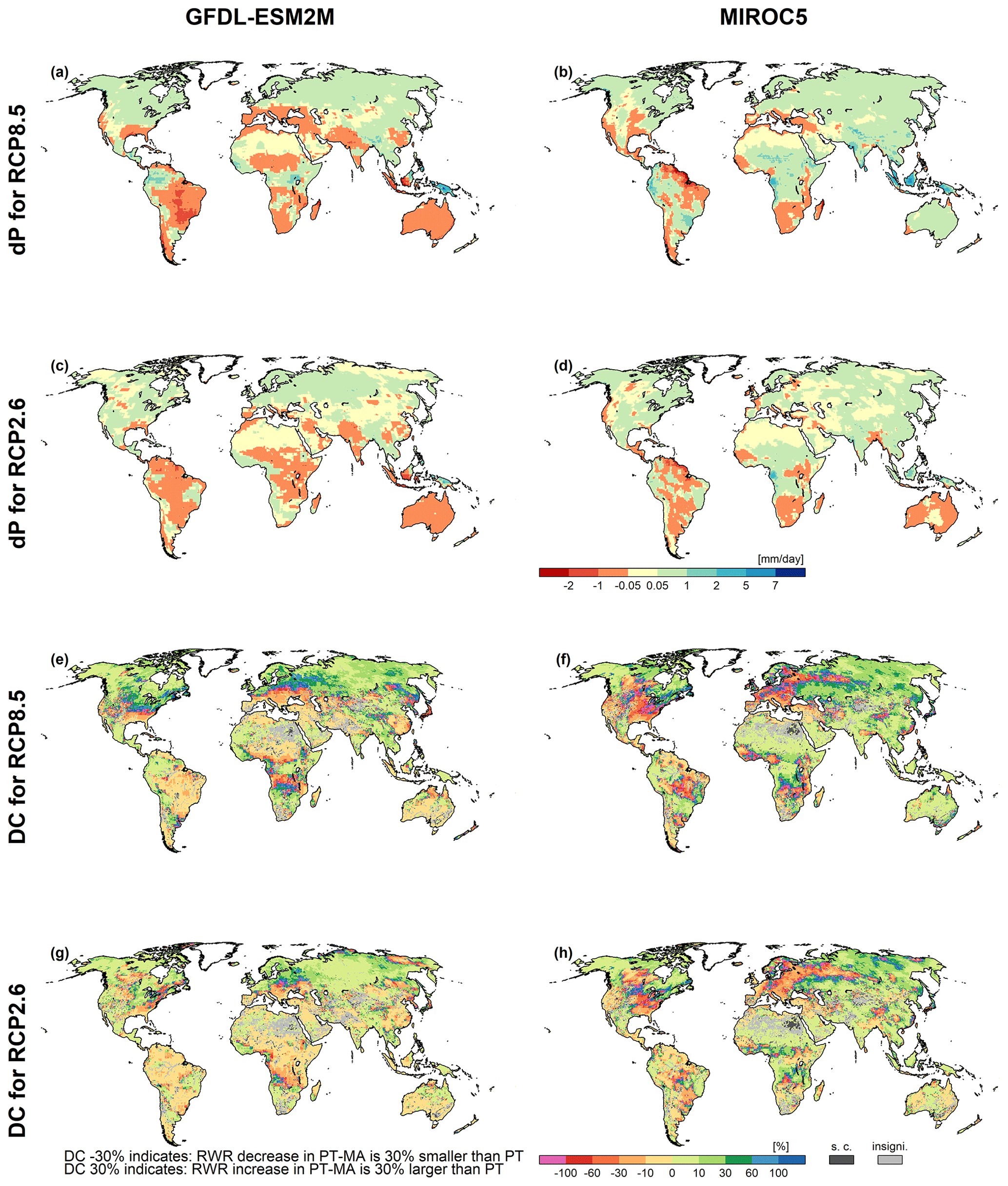
Figure B3 Precipitation (P) and the percent difference in dRWR-PT-MA and dRWR-PT (DC) changes for GFDL-ESM2M (a, c, e, g) and MIROC5 (b, d, f, h) climate data between the reference (1981–2000) and the future (2080–2099) periods under RCP8.5 and RCP2.6. The top four panels show the absolute change in average precipitation between future and reference periods (dP) for (a, b) RCP8.5 and (c, d) RCP2.6; the bottom four panels show the DC for (e, f) RCP8.5 and (g, h) RCP2.6. Cells where dRWR-PT-MA < dRWR-PT are denoted as special cases (“s.c.”). The cells labeled as “insigni.” represent instances where the computed change in RWR using the two methods is not statistically significant.

Appendix C: Abbreviations

Abbreviation	Definition
AET	Actual evapotranspiration
CMIP5	Coupled Model Intercomparison Project Phase 5
CO2	Carbon dioxide
DC	Relative difference of change
DGVM	Dynamic global vegetation model
GCM	Global climate model
MD	Milly and Dunne (2016)
NWSAET	Non-water-stressed actual evapotranspiration
PET	Potential evapotranspiration
PET-EO	Potential evapotranspiration derived from the energy-only method
PET-PM	Potential evapotranspiration derived from Penman–Monteith method
PET-PT-MA	Potential evapotranspiration derived from the Priestley–Taylor-modified approach (the new approach)
PM	Penman–Monteith
PT	Priestley–Taylor equation
PT-MA	Priestley–Taylor-modified approach (the new approach)
RCP	Representative Concentration Pathway
RWR	Renewable water resources
WGHM	WaterGAP Global Hydrological Model