Technical note: A procedure to clean, decompose, and aggregate time series

Errors, gaps, and outliers complicate and sometimes invalidate the analysis of time series. While most fields have developed their own strategy to clean the raw data, no generic procedure has been promoted to standardize the pre-processing. This lack of harmonization makes the inter-comparison of studies difficult, and leads to screening methods that can be arbitrary or case-specific. This study provides a generic pre-processing procedure implemented in R (ctbi for cyclic/trend decomposition using bin interpolation) dedicated to univariate time series. Ctbi is based on data binning and decomposes the time series into a long-term trend and a cyclic component (quantified by a new metric, the Stacked Cycles Index) to finally aggregate the data. Outliers are flagged with an enhanced box plot rule called Logbox that corrects biases due to the sample size and that is adapted to non-Gaussian residuals. Three different Earth science datasets (contaminated with gaps and outliers) are successfully cleaned and aggregated with ctbi. This illustrates the robustness of this procedure that can be valuable to any discipline.

1 Introduction

In any discipline, raw data need to be evaluated during a pre-processing procedure before performing the analysis. Errors are removed, values that deviate from the rest of the population are flagged (outliers, see Aguinis et al., 2013), and in some cases gaps are filled. Because the raw data are altered, pre-processing is a delicate and time-consuming task that can be neglected due to cognitive biases deflecting our understanding of reality (“I see what I want to see”), or due to our impatience to obtain results. The fate of extreme values is crucial, as they usually challenge scientific or economic theories (Reiss and Thomas, 2007).

Time series are particularly difficult to pre-process (Chandola et al., 2009). A value can or cannot be considered as an outlier just depending on its timestamp (e.g., a freezing temperature in summer), large data gaps are common, abrupt changes can occur, and a background noise covers the true signal. In Earth science, in situ or remote measurements routinely produce time series that first need to be visually inspected. The expert knowledge of the researcher, technician, or engineer is essential to flag suspicious periods of possible instrument failure (e.g., a rain gauge blocked by snowflakes), violation of the experimental conditions (e.g., a passing car during CO₂ measurements in a forest), or human error (e.g., calibration of the wrong sensor). Once these suspicious periods have been flagged, a pre-processing algorithm is necessary to evaluate the quality of the remaining portion of the measurements. However, there currently is no consensus on which procedure to use even in the simple univariate case: a recent review (Ranjan et al., 2021) covered more than 37 preprocessing methods for univariate time series, and Aguinis et al. (2013) listed 14 different outlier definitions that are mutually exclusive. Despite this (overwhelming) abundance of methods and conventions, there are surprisingly few R packages that offer a pre-processing function. It is worth mentioning hampel (package pracma, Borchers, 2021) that applies a Hampel filter (Pearson, 2002) to time series and flags outliers based on the mean absolute deviation (MAD), which is a robust approximation of the standard deviation defined as MAD$\left(x\right)=\mathrm{1.4826}\times \mathrm{M}(\mathrm{|}x-M(x\left)\mathrm{|}\right)$, with M the median operator. However, the hampel function is not robust to missing values and the scaling factor of 1.4826 is not adapted to non-Gaussian residuals. Another option is the function tsoutliers (package forecast, Hyndman and Khandakar, 2008) that applies a seasonal and trend decomposition using loess (STL, Cleveland et al., 1990) to data showing a seasonal pattern, complemented by a smoothing function to estimate the trend of non-seasonal time series (Friedman's super smoother, Friedman, 1984). The residuals obtained can be transformed to follow a Gaussian distribution (Cox–Box method, Box and Cox, 1964), and then outliers are flagged using the box plot rule (Tukey, 1977). This method will be proved in this study to work well with data associated with nearly-Gaussian residuals, but to show poor performance otherwise.

This study offers an alternative pre-processing procedure (implemented in R) called ctbi for cyclic/trend decomposition using bin interpolation. The time series is divided into a sequence of non-overlapping time intervals of equal period (called bins), and outliers are flagged with an enhanced version of the box plot rule (called Logbox) that is adapted to non-Gaussian data for different sample sizes. Ctbi fulfills four purposes as follows:

• i.

  Data cleaning. Bins with insufficient data are discarded, and outliers are flagged in the remaining bins. If there is a cyclic pattern within each bin, missing values can be imputed as well.

• ii.

  Decomposition. The time series is decomposed into a long-term trend and a cyclic component.

• iii.

  Cyclicity analysis. The mean cycle of the stacked bins is calculated, and the strength of the cyclicity is quantified by a novel index, the Stacked Cycles Index.

• iv.

  Aggregation. Data are averaged (or summed) within each bin.

This procedure is particularly adapted to univariate time series that are messy, with outliers, data gaps, or irregular time steps. The inputs offer a large flexibility in terms of imputation level or outlier cutoff, but also in the timestamp of the bins: a day does not necessarily start at midnight or a year the 1 January. The timeline is not limited to daily or monthly data, but can vary from milliseconds to millenaries. The outputs keep track of the changes brought to the data: contaminated bins are flagged as are outliers and imputed data points.

This paper is divided into two distinct parts. The first part describes the Logbox method, and compares its performance with five other outlier detection methods in the literature based on daily precipitation and temperature data extracted from century-old weather stations. The second part describes the ctbi procedure, and then applies it to three datasets that have been contaminated beforehand to show the efficiency of the algorithm. A comparison with tsoutliers is performed, and, finally, limitations and good practice recommendations are discussed.

2 Part I: outliers

2.1 Context

This first part is dedicated to the detection of outliers present in univariate datasets (without the time component). The box plot (or Tukey's) rule is a commonly used method to flag outliers below a lower boundary l and above an upper boundary u (Tukey, 1977):

$$\begin{array}{}\text{(1)}& \left\{\begin{array}{l}l=q\left(\mathrm{0.25}\right)-\mathit{\alpha }\times \left(q\left(\mathrm{0.75}\right)-q\left(\mathrm{0.25}\right)\right)\\ u=q\left(\mathrm{0.75}\right)+\mathit{\alpha }\times \left(q\left(\mathrm{0.75}\right)-q\left(\mathrm{0.25}\right)\right)\end{array}\right.,\end{array}$$

with q the sample quantile (e.g., q(0.5) is the median) and α=1.5 a constant that corresponds to 99.3 % of Gaussian data falling within [l,u]. This method is simple and robust to the presence of a maximum of 25 % of outliers in the dataset (known as the breakdown point). When a real data point falls outside the [l,u] range, it is considered as an erroneously flagged outlier (or type I error). Conversely, a type II error occurs when a real outlier is not flagged. The type I error is more common for three reasons as follows:

• i.

  For small Gaussian samples (n < 30), up to 8.6 % of data (Hoaglin et al., 1986) can be cut due to the inaccuracy of the sample quantile for small n.

• ii.

  For large Gaussian samples (n>10³), α=1.5 is inappropriate because the number of erroneously flagged outliers increases linearly with n due to the 99.3 % of data captured by [l,u].

• iii.

  For non-Gaussian populations, α=1.5 is generally too restrictive. For example, ∼4.8 % of data following an exponential distribution would be cut.

Studies have corrected biases in the detection of outliers in small samples (see Carling, 2000; Schwertman et al., 2004) and large samples (Barbato et al., 2011), but these methods were adapted to Gaussian populations. For non-Gaussian populations, Kimber (1990) and Hubert and Vandervieren (2008) have adjusted α to the skewness (related to the asymmetry of a distribution), but did not consider the kurtosis (related to the tail weight) that will be proven to be a key variable in this study. Therefore, there currently is no generic procedure that can be used when the population is non-Gaussian.

To understand how to address this problem, two sets of common distributions with known skewness S, kurtosis excess κ_ex, and quantile function Q are used (Fig. 1). The first set is the Pearson family composed of light-tailed distributions that represent any theoretically possible residuals with moderate S and κ_ex. Pearson originally worked to create distributions that cover the entire (S, κ_ex) space (Pearson, 1895, 1901, 1916), but they took their modern names later on (gamma, inverse gamma, beta prime, Student, Pearson IV). The second set is the generalized extreme value (GEV) family composed of the Gumbel, Weibull, and Fréchet that are heavy-tailed distributions (high S and κ_ex) used in extreme value theory to model the behavior of extrema (Jenkinson, 1955). Based on this framework, this study finds that $\mathit{\alpha }\left(n\right)=A\log \left(n\right)+B+\frac{C}{n}$ reasonably addresses all previously mentioned issues, with C fixed as a constant (C=36). The two parameters A and B correspond to the nature of the distribution, and are estimated based on a predictor of the maximum tail weight and inspired by Moors (1988). A comparison between this procedure (called Logbox) and five other existing models is performed on residuals obtained from 6307 weather stations with more than 100 years of daily temperature and precipitation measurements (Fig. 2). Finally, Logbox is implemented in part II to clean the residuals obtained after fitting the univariate time series with a robust and nonparametric method.

Figure 1 Location of the 4999 light-tailed distributions of the Pearson family (a) and the 368 heavy-tailed distributions of the GEV family (d) in the (κ_ex,S²) space (kurtosis excess, squared skewness). The coefficients A and B correspond to $\mathit{\alpha }\left(n\right)=A\times \log \left(n\right)+B+\frac{\mathrm{36}}{n}$ used to replace α=1.5 in the box plot rule. For the Pearson family, they are shown in the (κ_ex,S²) space (b, c). For the GEV family (e, f), they are shown against a predictor of the maximum tail weight defined for right-skewed distributions as $m_{*}=(E_{\mathrm{7}}-E_{\mathrm{5}})/(E_{\mathrm{6}}-E_{\mathrm{2}})-\mathrm{0.6165}$, with $E_i=q(i/\mathrm{8})$ the sample octile.

2.2 Method

2.2.1 Distributions

Residuals with moderate κ_ex and S are represented in this study with 4999 light-tailed distributions from the Pearson family (Pearson, 1895, 1901, and 1916) composed of the Gaussian, gamma (196 distributions, including the exponential), inverse gamma (170), beta prime (1135), Pearson IV (3377), and Student (120) distributions (Fig. 1a). These distributions cover the entire (κ_ex,S²) space without overlap, except for the beta distribution that has been discarded due to a bounded support (unrealistic residuals). The shape parameters of each distribution have been chosen to produce regularly spaced points with a mean distance of 0.05 in the (κ_ex,S²) space, and with a range between the Gaussian and the exponential: ${\mathit{\kappa }}_{\mathrm{ex}}\in [\mathrm{0},\mathrm{6}]$ and $S\in [\mathrm{0},\mathrm{2}]$. Heavy-tailed residuals are represented with 368 distributions from the generalized extreme value (GEV) family (Fig. 1d) composed of the Gumbel, Weibull (244 distributions), and Fréchet (123). Their shape parameters cover a larger range: ${\mathit{\kappa }}_{\mathrm{ex}}\in [\mathrm{0},\mathrm{500}]$ and $S\in [\mathrm{0},\mathrm{15}]$.

2.2.2 The Logbox model

Based on the box plot rule, α can be defined as

$$\begin{array}{}\text{(2)}& \mathit{\alpha }\left(n\right)={\displaystyle \frac{Q\left(\mathrm{1}-\frac{f\left(n\right)}{\mathrm{2}n}\right)-Q\left(\mathrm{0.75}\right)}{Q\left(\mathrm{0.75}\right)-Q\left(\mathrm{0.25}\right)}},\end{array}$$

with n the sample size, Q the population quantile function, and f a function that gives the number of erroneously flagged outliers. In the original box plot rule, $Q={\mathrm{\Phi }}^{-\mathrm{1}}$ (with Φ the cumulative distribution function of the Gaussian) and f(n)=0.007n, which leads to α=1.5. As explained in the introduction, this choice of f is not valid for large sample sizes due to the linear dependence on n. A flat number of erroneously flagged outliers (f(n)=b) or a logarithmic relationship (f(n)=b log(n)) would not be appropriate either, because α(n) could take arbitrary large values as $\mathrm{1}-\frac{f\left(n\right)}{\mathrm{2}n}$ would approach 1 too rapidly (Q(1)=∞). This study suggests instead $f\left(n\right)=\mathrm{0.001}\sqrt{n}$ as a compromise. For example, for a sample of size n=10², 10⁴ or 10⁶, respectively 0.01, 0.1, or 1 point would be erroneously flagged as outlier (instead of 0.7, 70, or 7000 points with the original box plot rule). To characterize the relationship α(n) versus n, α is derived with high accuracy (Q implemented in R) for each distribution of the Pearson and GEV family for five sample sizes (n_i=10ⁱ with $i\in [\mathrm{2},\mathrm{6}]$). It appears that $\mathit{\alpha }\left(n\right)=A\log \left(n\right)+B$ is an accurate model for both the Pearson family (mean of $r^{\mathrm{2}}=\mathrm{0.994}\pm \mathrm{0.005}$) and the GEV family ($r^{\mathrm{2}}=\mathrm{0.99}\pm \mathrm{0.01}$). Barbato et al. (2011) found the same law for the Gaussian distribution based on empirical considerations only, with reported values of A=0.15 and B=1.15. For comparison, this study finds A=0.08 and B=2 for the Gaussian distribution (r²=0.999).

The relationship $\mathit{\alpha }\left(n\right)=A\log \left(n\right)+B$ now needs to be extended to small or non-Gaussian samples. To account for biases emerging at small sample size, an additional term is added following Carling (2000): $\mathit{\alpha }\left(n\right)=A\log \left(n\right)+B+\frac{C}{n}$. The parameter C=36 has been numerically determined with a Monte Carlo simulation on the distributions of the Pearson family to ensure that the percentage of erroneously flagged outliers corresponds to ∼0.1 % for n=9 (Supplement). To account for non-Gaussian populations, A and B will be estimated with a new robust predictor sensitive to the tail weight. Let (m₋, m₊) be two functions defined as $m_{-}=(E_{\mathrm{3}}-E_{\mathrm{1}})/(E_{\mathrm{6}}-E_{\mathrm{2}}$) and $m_{+}=(E_{\mathrm{7}}-E_{\mathrm{5}})/(E_{\mathrm{6}}-E_{\mathrm{2}})$, with $E_i=q(i/\mathrm{8})$ the sample octile. The centered Moors $m=m_{-}+m_{+}-\mathrm{1.23}$ is a known robust predictor of the kurtosis excess with a breakdown point of 12.5 % (Moors, 1988; Kim and White, 2004). However, this study introduces a modified version defined as $m_{*}=\max (m_{-},m_{+})-\mathrm{0.6165}$. The parameter m_* is more appropriate than m to determine if a sample is light-tailed or heavy-tailed. For example, a Gaussian distribution ($m_{-}=m_{+}\approx \mathrm{0.6165}$) and a right-skewed distribution with one heavy tail ($m_{-}=\mathrm{0.1}$ and $m_{+}=\mathrm{1.13}$) will share identical m but different m_*. The relationships shown in Fig. 1 are $A=g_A\left(m_{*}\right)$ and $B=g_B\left(m_{*}\right)$, with $g_A\left(x\right)=\mathrm{0.2294}{e}^{\mathrm{2.9416}x-\mathrm{0.0512}{x}^{\mathrm{2}}-\mathrm{0.0684}{x}^{\mathrm{3}}}$ (r²=0.999) and $g_B\left(x\right)=\mathrm{1.0585}+\mathrm{15.6960}x-\mathrm{17.3618}{x}^{\mathrm{2}}+\mathrm{28.3511}{x}^{\mathrm{3}}-\mathrm{11.4726}{x}^{\mathrm{4}}$ (r²=0.999) for $x\in [\mathrm{0},\mathrm{2}]$. Each function has been parameterized based on the Pearson and GEV family together (Fréchet has been excluded due to a different behavior). The coefficients have been determined with a Monte Carlo simulation that minimizes the root mean square error (N∼10⁸).

For an unknown sample of size n≥9, the Logbox procedure is finally the following: m_* is computed (bounded by [0,2]) and the box plot rule is used, with $\mathit{\alpha }\left(n\right)=g_A\left(m_{*}\right)\log \left(n\right)+g_B\left(m_{*}\right)+\frac{\mathrm{36}}{n}$.

2.2.3 Former models

Logbox is compared to five other models (Kimber, 1990; Hubert and Vandervieren, 2008; Schwertman et al., 2004; Leys et al., 2013; Barbato et al., 2011). The first two models (Kim. and Hub.) adjust the box plot method with respect to the skewness as follows:

$$\begin{array}{}\text{(3)}& \left\{\begin{array}{l}{l}_{\mathrm{Kim}.}=q\left(\mathrm{0.25}\right)-\mathrm{3}\times \left(q\left(\mathrm{0.50}\right)-q\left(\mathrm{0.25}\right)\right)\\ u_{\mathrm{Kim}.}=q\left(\mathrm{0.75}\right)+\mathrm{3}\times \left(q\left(\mathrm{0.75}\right)-q\left(\mathrm{0.50}\right)\right)\end{array}\right.,\end{array}$$

and

$$\begin{array}{}\text{(4)}& \left\{\begin{array}{l}{l}_{\mathrm{Hub}.}=q\left(\mathrm{0.25}\right)-\mathrm{1.5}\times h(-\mathrm{MC})\\ \times \left(q\left(\mathrm{0.75}\right)-q\left(\mathrm{0.25}\right)\right)\\ u_{\mathrm{Hub}.}=q\left(\mathrm{0.75}\right)+\mathrm{1.5}\times h\left(\mathrm{MC}\right)\\ \times \left(q\left(\mathrm{0.75}\right)-q\left(\mathrm{0.25}\right)\right)\end{array}\right.,\end{array}$$

with the function h defined as h(MC)=e^4MC for MC < 0 and h(MC)= e^3MC for MC ≥ 0. The Medcouple $\mathrm{MC}\in [-\mathrm{1},\mathrm{1}]$ is a robust estimator of S, with an algorithm complexity of O(n log  n) and a breakdown point of 25 % (Brys et al., 2004). The third model (Sch.) constructs the lower and upper boundary around the median,

$$\begin{array}{}\text{(5)}& \left\{\begin{array}{l}{l}_{\mathrm{Sch}.}=q\left(\mathrm{0.50}\right)-\frac{Z}{k_n}\times \mathrm{2}\left(q\left(\mathrm{0.50}\right)-q\left(\mathrm{0.25}\right)\right)\\ u_{\mathrm{Sch}.}=q\left(\mathrm{0.50}\right)+\frac{Z}{k_n}\times \mathrm{2}\left(q\left(\mathrm{0.75}\right)-q\left(\mathrm{0.50}\right)\right)\end{array}\right.,\end{array}$$

with k_n a function of the sample size n to adjust for small samples (given as a table in Schwertman et al., 2004) and Z a constant related to the percentage of data captured by $[l_{\mathrm{Sch}.},u_{\mathrm{Sch}.}]$, here picked as Z=3 (Gaussian case for the ±3σ window). The fourth model (Ley.) uses the MAD around the median,

$$\begin{array}{}\text{(6)}& \left\{\begin{array}{l}{l}_{\mathrm{Ley}.}=q\left(\mathrm{0.50}\right)-\mathrm{3}\times \mathrm{MAD}\\ u_{\mathrm{Ley}.}=q\left(\mathrm{0.50}\right)+\mathrm{3}\times \mathrm{MAD}\end{array}\right..\end{array}$$

Finally, the last model (Bar.) is similar to the Logbox procedure but parameterized on the Gaussian distribution only,

$$\begin{array}{}\text{(7)}& \left\{\begin{array}{l}{l}_{\mathrm{Bar}.}=q\left(\mathrm{0.25}\right)-(\mathrm{0.15}\times \log \left(n\right)+\mathrm{1.15})\times \left(q\left(\mathrm{0.75}\right)\right.\\ \left.-q\left(\mathrm{0.25}\right)\right)\\ u_{\mathrm{Bar}.}=q\left(\mathrm{0.75}\right)+(\mathrm{0.15}\times \log \left(n\right)+\mathrm{1.15})\times \left(q\left(\mathrm{0.75}\right)\right.\\ \left.-q\left(\mathrm{0.25}\right)\right)\end{array}\right..\end{array}$$

2.2.4 Comparison between models

The comparison between models is performed on two sets of residuals obtained from weather stations part of the Global Historical Climatology Network (GHCN-daily) with at least 100 years of daily temperature (2693 stations, 9.4×10⁷ d) or daily precipitation (6277 stations, 5.8×10⁷ wet days, dry days are excluded). Because this network is used to calibrate products that are remote-sensing-based and because suspicious values are routinely flagged (Menne et al., 2012a), the risk of errors in these century-old stations can be considered small. The residuals are extracted with the robust method described in part II based on non-overlapping bins (bins with less than 80 % of data are discarded). To reduce the impact of the extraction method on the analysis, three bin intervals (5, 10, and 20 d) are used to obtain three replicas for each station. The sensitivity of each outlier detection method to the sample size has also been estimated. For each station and for each sample size l_i=10i (i varying from 1 to 10), $N_i=\frac{\mathrm{100}}{i}$ samples are randomly selected, and the number of flagged outliers is summed over all the N_i samples (the total number of points is constant, $N_i\times l_i=\mathrm{1000})$.

For the five models (Ley., Hub., Kim., Sch., Bar.), the percentage of flagged outliers is computed for each station, and then the mean (±1 SD) is calculated over all stations. For the Logbox model, this method is not appropriate because the expected number of erroneously flagged outlier per station is less than 1 ($\mathrm{0.001}\sqrt{\sim {\mathrm{10}}^{\mathrm{4}}}\sim \mathrm{0.1})$. Instead, the percentage of flagged outliers is calculated over the total number of points: $\mathit{\rho }=\left(\mathrm{\Sigma }{n}_j^{\mathrm{flagged}}\right)\times \mathrm{100}/\left(\mathrm{\Sigma }{n}_j\right)$, with j a station. The variability is estimated by subsampling the total number of stations N_s: $\sqrt{N_{\mathrm{s}}}$ sets of $\sqrt{N_{\mathrm{s}}}$ random stations are selected without replacement. The parameter ρ is computed for each set, and the associated variability is calculated on all ρ values (±1 SD in Fig. 2f and quantiles in Fig. 2c).

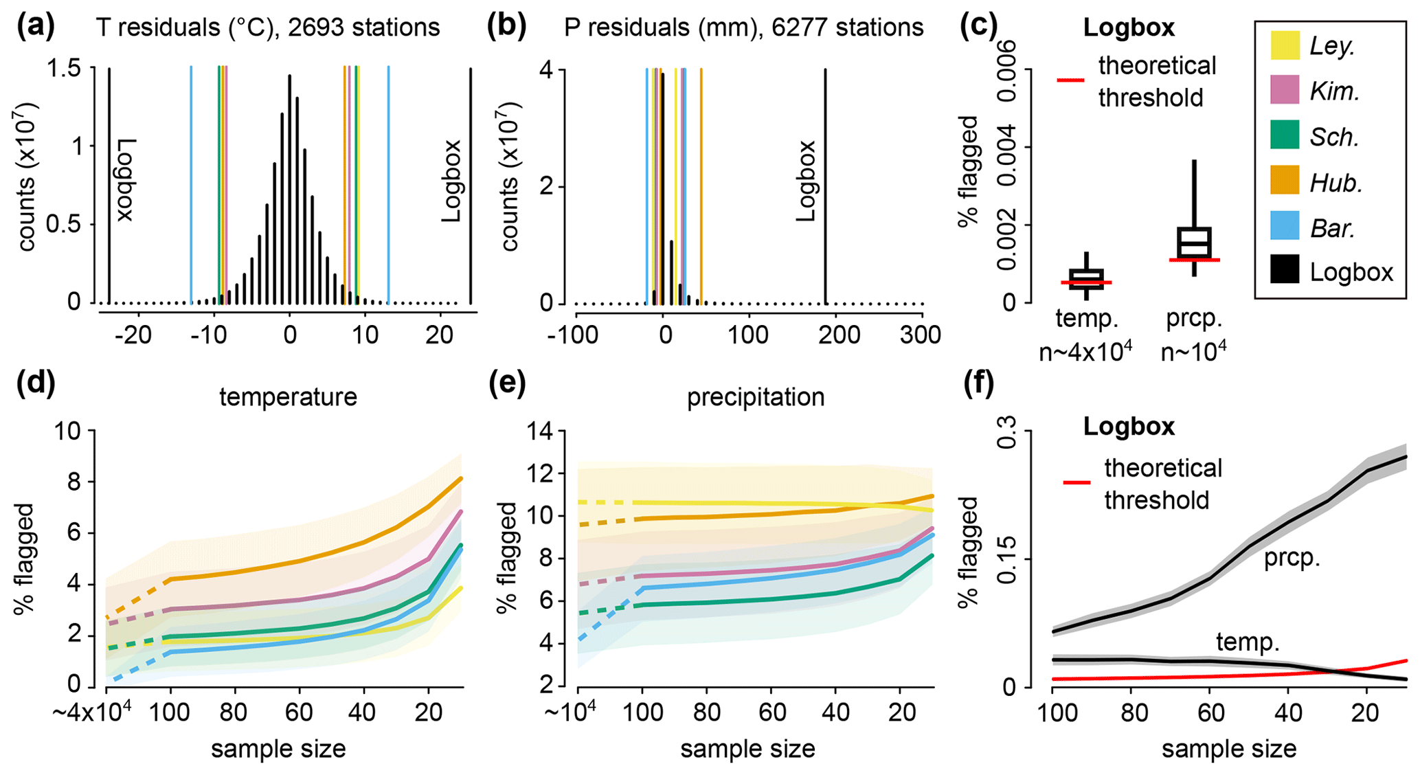
Figure 2 Comparison between six outlier detection methods performed on two sets of residuals (temperature and precipitation) obtained from weather stations with daily measurements over at least 100 years. The two histograms (a, b) represent aggregated residuals from all stations (for visualization purpose only) and show counts with at least 100 daily occurrences, with the median of the lower/upper threshold displayed for each method. For the methods Ley. (Leys et al., 2013), Kim. (Kimber, 1990), Sch. (Schwertman et al., 2004), Hub. (Hubert and Vandervieren, 2008), and Bar. (Barbato et al., 2011), the mean percentage (±1 SD) of flagged data is shown for sample sizes varying from 10 to 100, and for all available points per station ($n\sim \mathrm{4}\times {\mathrm{10}}^{\mathrm{4}}$ for the temperature and n∼10⁴ for the precipitation, panels d and e). For Logbox (c, f), this percentage is calculated by pooling all points, and the variability is estimated with a random resampling of stations (see Method). The theoretical threshold is the expected percentage of erroneously flagged outliers ($p_{\mathrm{theo}}=f\left(n\right)\times \frac{\mathrm{100}}{n}=\frac{\mathrm{0.1}}{\sqrt{n}}\mathit{\%}$).

2.3 Results and discussion

The parameter α=1.5 used in the box plot rule is sensitive to the sample size n, and the relationship $\mathit{\alpha }\left(n\right)=A\log \left(n\right)+B+\frac{C}{n}$ corrects for this effect for both light-tailed distributions (Pearson family, Fig. 1a) and heavy-tailed distributions (GEV family, Fig. 1d). The value of A,B, and C depends on the outlier threshold level and the nature of the distribution. The convention in this study is to set the expected number of erroneously flagged outliers to $f\left(n\right)=\mathrm{0.001}\sqrt{n}$, which corresponds to a percentage of type I error of $\mathrm{0.1}/\sqrt{n}$ %. This leads to homogeneous A and B values among the Pearson family ($A=\mathrm{0.8}\pm \mathrm{0.3}$, $B=\mathrm{3}\pm \mathrm{1}$, Fig. 1b, c) used to numerically determine C=36 (Supplement). Because the value of A and B rapidly diverges for heavy-tailed distributions, a model adapted to the shape of the residuals is required (Fig. 1e, f). To keep this model simple, the asymmetry of a distribution (i.e., the skewness) is ignored in this study in order to only focus on the weight of the heavier tail. Possible outliers might not be flagged on the light tail of an asymmetric distribution (risk of type II error), but residuals with strong asymmetry are usually produced when the range of possible values is semi-bounded (e.g., precipitation in $[\mathrm{0},+\mathrm{\infty }[)$, which makes the detection of errors trivial (negative precipitation). For this purpose, the parameter m_* is a robust predictor of the maximum tail weight with a breakdown point of 12.5 %. Finally, $\mathit{\alpha }\left(n\right)=g_A\left(m_{*}\right)\log \left(n\right)+g_B\left(m_{*}\right)+\frac{\mathrm{36}}{n}$ for n≥9 and $m_{*}\in \left[\mathrm{0},\mathrm{2}\right]$, with the functions g_A and g_B parameterized on both families (Fig. 1e, f). The Fréchet distribution has been excluded because its tails are decaying too rapidly (the A and B coefficients are bounded despite an extreme kurtosis).

The Logbox procedure is tested and compared with five other models on daily precipitation and temperature residuals from century-old weather stations (Fig. 2). It is firstly visually striking that the outlier threshold from the five traditional methods cut too many data points not only for the precipitation but also for the temperature residuals (Fig. 2a, b). The percentage of flagged data points per station varies around 1.7±1 % for the temperature (Fig. 2d, median of $\mathrm{36}\mathrm{634}\approx \mathrm{4}\times {\mathrm{10}}^{\mathrm{4}}$ d per station), and from 4.1 % (Bar.) to 10.5 % (Ley.) for the precipitation (Fig. 2e, median of 8352≈10⁴ wet days per station).

The reason for the large discrepancy between observed and expected percentage of flagged outliers (∼0.7 % based on the box plot rule) is that these methods have been designed for nearly-Gaussian residuals. Even daily temperatures are diverging from normality because the fitting model used to extract residuals from the time series minimizes the root mean square error. The anomalies are therefore more concentrated around 0 than those produced by a Gaussian, but with larger extremes (Fig. 2a, leptokurtic distribution). Only the Bar. model correctly captures outliers present in the temperature residuals (0.17 % data points flagged), as it accounts for large sample size effects (logarithmic law in α similar to Logbox). However, Bar. fails at capturing outliers in the precipitation residuals because this method has been parameterized on the Gaussian only. For small samples, the type I error is even higher in all traditional methods due to the inaccuracy of the quantiles: from 1.4 % (Bar.) to 4.2 % (Hub.) of temperature residuals are cut for n=100 (Fig. 2d). This analysis proves that none of the former methods are suitable to detect outliers in non-Gaussian residuals.

In comparison, the Logbox procedure shows a percentage of flagged outliers close to the expected values for large sample sizes (Fig. 2c), with 0.0006±0.0003 % for the temperature (expected value of 0.0005 %) and 0.0017±0.0009 % for the precipitation (expected value of 0.001 %). These results are surprisingly accurate knowing that 12.5 % of the extreme values are disregarded for robustness reasons (m_*), and also knowing that Logbox has only been parametrized on theoretical distributions (Pearson and GEV family). For smaller sample sizes (n < 30 in Fig. 2f), the precipitation residuals are cut too frequently (∼0.25 %) compared to the expected threshold (∼0.03%), but the temperature residuals are not cut enough. The constant parameter used to correct for a sample size effect (C=36) is only adapted to nearly-Gaussian residuals, and it cannot be better estimated because any predictor (such as m_*) becomes inaccurate at smaller sample sizes. However, the percentage of flagged outliers remains within 1 order of magnitude of the expected threshold, which is a reasonable compromise between type I errors (precipitation) and type II errors (temperature).

To summarize, Logbox enhances the box plot rule by considering the sample size effect and by adapting the cutting thresholds to the data. This method has been implemented in the function ctbi.outlier (in the R package ctbi) that will be used to flag potential outliers in the residuals obtained by the aggregation procedure described in part II.

3 Part II: the ctbi procedure

3.1 Context

This second part is dedicated to the pre-processing, partial imputation, and aggregation of univariate time series. In order to flag outliers, one first needs to produce residuals that represent the variability around the signal. In its simplest form, the time series y_t is represented with the following additive decomposition (Hyndman and Athanasopoulos, 2021): $y_{\mathrm{t}}=T_{\mathrm{t}}+S_{\mathrm{t}}+{\mathit{ϵ}}_{\mathrm{t}}$, with T_t a long-term trend, S_t a cyclic component (originally seasonal component, but the term cyclic is preferred here as it is more generic), with period τ (∀t, $S_{\mathrm{t}}=S_{\mathrm{t}+\mathit{\tau }})$ and ε_t the residuals that are considered to be stationary. A popular algorithm that performs this decomposition is the seasonal and trend decomposition using loess (or STL, Cleveland et al., 1990), that is robust to the presence of outliers. The enhanced version of the algorithm, STLplus (Hafen, 2016), is also robust to the presence of missing values and data gaps. Unfortunately, there are three major drawbacks to using STLplus in the general case: (i) this algorithm has specifically been designed for signals showing seasonal patterns, which makes it less relevant for other types of data; (ii) the long-term trend based on loess needs several input parameters (s.window, s.degree, etc.), and the decomposition is therefore not unique; and (iii) the algorithm has a complexity of O(n²) due to the loess, which is resource intensive and not adapted to long time series (n > 10⁷). In particular, the first point explains why the function tsoutliers needs to use a smoothing function (Friedman, 1984) to complement the STL procedure.

A new robust and nonparametric procedure (ctbi) is proposed instead to calculate T_t and S_t using non-overlapping bins. Outliers are flagged in the residuals ϵ_t with the Logbox method described in part I, and imputation is performed using T_t+S_t if the cyclic pattern is strong enough, which is quantified by a new index introduced in this study (the Stacked Cycles Index or SCI). Bins with sufficient data can finally be aggregated, while other bins are discarded. The procedure is simple (entirely described in Fig. 3), the long-term trend T_t is unique and non-parameterized (based on linear interpolations crossing each bin), and the cyclic component S_t is simply the mean stack of bins using detrended data (equivalent to STL for periodic time series). The algorithm complexity is of the order of O(n log (n)) because the loess is not necessary anymore. In the following, the procedure is first described more in details and then applied to three case studies (a temperature, precipitation, and methane dataset) that have been contaminated with outliers, missing values, and data gaps. Comparison with the raw data demonstrates the reliability of the ctbi procedure, whose performance is compared to tsoutliers.

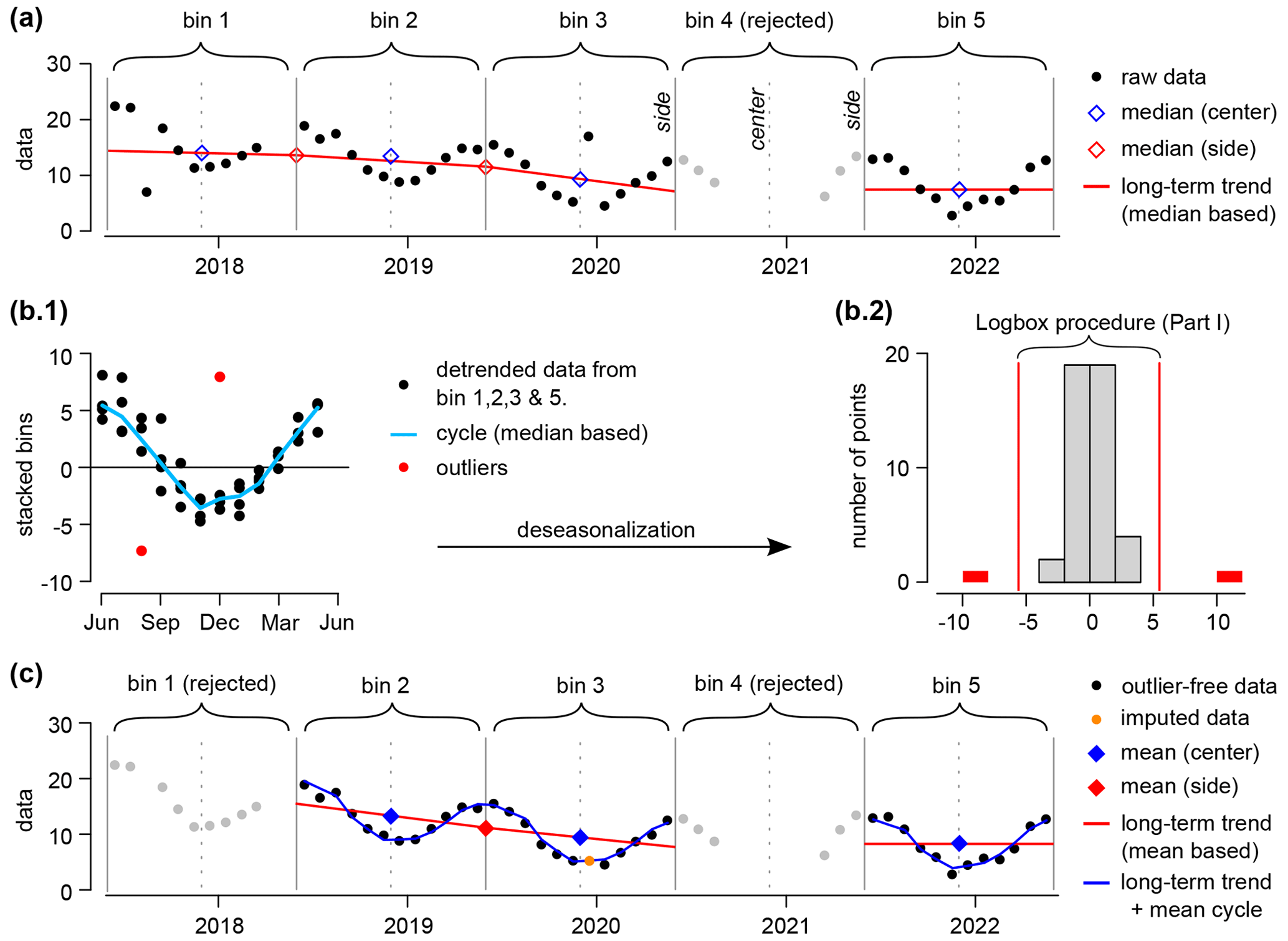
Figure 3 Example of the aggregation procedure with the following inputs: bin side = 1 June 2020, bin period = 1 year, f_NA=0.2 (minimum of 10 months of data for a bin to be accepted), and SCI_min=0.6 (cyclic imputation level). The bin 4 has been rejected because it contains only 6 months of data (a). Two outliers have been flagged in the residuals (detrended and deseasonalized data, b.2). After the outliers have been replaced with NA values, the bin 1 has been rejected (9 months of data), and the long-term trend and cycle have been updated using the mean instead of the median (c). A point in bin 3 has been imputed based on the cyclicity (${\mathrm{SCI}}_{\min }\le \mathrm{SCI}=\mathrm{0.61}$).

3.2 Method

3.2.1 Definitions

Bin

A bin is a time window characterized by a left side (inclusive), a right side (exclusive), a center, and a period (e.g., 1 year in Fig. 3a). Any univariate time series can be decomposed in a sequence of non-overlapping bins, with the first and last data point contained in the first and last bin, respectively (Fig. 3a). The bin size n_bin is the rounded median of the number of points (including “Not Available”, or “NA”, values) present in each non-empty bin. A bin is accepted when its number of non-NA data points is above n_bin(1−f_NA) with $f_{\mathrm{NA}}\in [\mathrm{0},\mathrm{1}]$ the maximum fraction of NA values per bin (input left to the user). Otherwise, the bin is rejected and all its data points are set to NA (Fig. 3a, bin 4).

Long-term trend

The long-term trend (median-based) is a linear interpolation of the median values associated with each side (calculated between two consecutive centers, see Fig. 3a). A side value is set as missing if the number of non-NA data points (between the two nearest consecutive centers) is below n_bin(1−f_NA). To solve for boundaries issues and missing sides values, the interpolation is extended using the median value associated with each center (bin 1, 3, and 5 in Fig. 3a). Once the outliers have been quarantined, the long-term trend (mean-based) will be calculated following the same method, but using the mean instead of the median (Fig. 3c).

Cycle

The cycle (median-based) is composed of n_bin points that are the medians of the stack of all accepted bins with the long-term trend (median based) removed (Fig. 3b1). Once the outliers have been quarantined, the cycle (mean-based) will be the mean stack of accepted bins with the long-term trend (mean-based) removed (bin 2, 3, and 5 in Fig. 4a). The cyclic component S_t is the sequence of consecutive cycles.

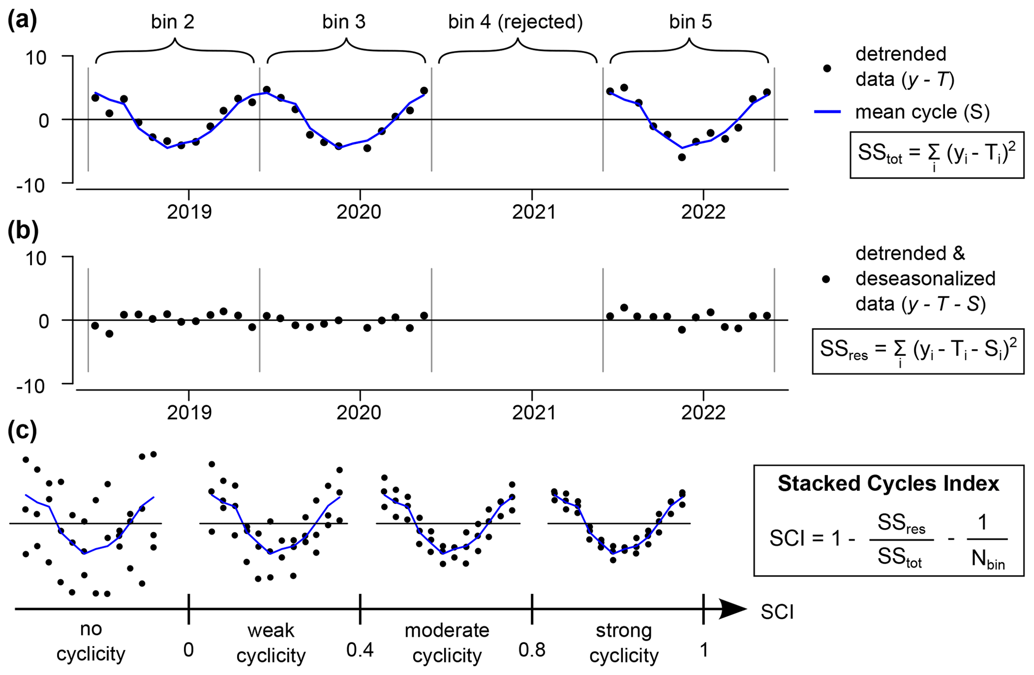
Figure 4 The Stacked Cycles Index (SCI ≤ 1) quantifies the strength of the cyclicity associated with the period of a bin. The long-term trend (mean-based) is first removed to compute the total sum of squares (a). Then the cyclic component (mean-based) is also removed to compute the sum of squared residuals (b). SCI is the coefficient of determination minus $N_{\mathrm{bin}}^{-\mathrm{1}}$, to correct for a bias emerging at a small number of bins, with N_bin the number of accepted bins (here, N_bin=3, c).

Stacked Cycles Index

SCI ≤1 is an adimensional parameter quantifying the strength of a cycle based on the variability around the mean stack (Fig. 4). Its structure is similar to another index developed in a former study (Wang et al., 2006), however a factor of $N_{\mathrm{bin}}^{-\mathrm{1}}$ has been added to correct for a bias emerging at a small number of bins (N_bin is the number of accepted bins). This correcting factor has been calculated based on stationary time series of Gaussian noise (with therefore a null cyclicity per definition, see Supplement).

3.2.2 Ctbi procedure

Inputs

1. The univariate time series (first and second column: time and raw data, respectively).

2. One bin center or one bin side (e.g., 1 June 2020).

3. The period of the bin (e.g., 1 year).

4. The aggregation operator (mean, median, or sum).

5. The range of possible values (default value $y_{\lim }\in ]-\mathrm{\infty },+\mathrm{\infty }[)$.

6. The maximum fraction of NA values per bin (default value f_NA=0.2).

7. The $A,B,C$ coefficients used in the Logbox method (automatically calculated by default, coeffoutlier='auto').

8. The minimum SCI for imputation (default value SCI_min=0.6).

Outputs

1. The original dataset with nine columns: (i) time; (ii) outlier-free and imputed data; (iii) index of the bins associated with each data points (the index is negative if the bin is rejected); (iv) long-term trend; (v) cyclic component; (vi) residuals (including the outliers); (vii) quarantined outliers; (viii) value of the imputed data points; and (ix) relative position of the data points in their bins between 0 (the point falls on the left side) and 1 (the point falls on the right side).

2. The aggregated dataset with 10 columns: (i) aggregated time (center of the bins); (ii) aggregated data; (iii) index of the bin (negative value if the bin is rejected); (iv) start of the bin; (v) end of the bin; (vi) number of points per bin (including NA values); (vii) number of NA values per bin, originally; (viii) number of outliers per bin; (ix) number of imputed points per bin; and (x) variability associated with the aggregation (standard deviation for the mean, MAD for the median, and nothing for the sum).

3. The mean cycle with three columns: (i) time boundary of the first bin with n_bin points equally spaced; (ii) the mean value associated with each point; and (iii) the standard deviation associated with the mean value.

4. A summary of the bins: the Stacked Cycles Index (SCI), the representative number of data points per bin (n_bin), and the minimum number of data points for a bin to be accepted (n_bin min).

5. A summary of the Logbox output: the coefficients A, B, and C, m_*, the number of points used, and the lower/upper outlier threshold.

Step 1: data screening

The bin size n_bin is calculated; values above or below y_lim are set to NA; the number of accepted bins N_bin is assessed; all data points within rejected bins are set to NA; and the long-term trend and cycle (both median based) are calculated (Fig. 3a, b1).

Step 2: outliers

Outliers are flagged in the residuals (detrended and deseasonalized data) using Logbox (Fig. 3b2); outliers are quarantined and their values are set to NA; the number of accepted bins N_bin is updated; and all data points within newly rejected bins are set to NA (bin 1 in Fig. 3c).

Step 3: long-term trend and cycle (mean based)

The long-term trend and the cycle are calculated using the mean instead of the median (Fig. 3c); and SCI is calculated (Fig. 4).

Step 4: imputation

If SCI>SCI_min, all NA values in accepted bins are imputed with the long-term trend + the mean cycle (imputation bounded by y_lim). Repeat step 3 and step 4 three times to reach convergence.

Step 5: aggregation

Accepted bins are aggregated around their center.

3.2.3 Case studies

Three univariate datasets are chosen to illustrate the potential of the aggregation procedure (Fig. 5, first column). The first dataset is an in situ temperature (in ^∘C) measured during summer in the canopy of an Oak woodland of California (month of August, temporal resolution of 5 min) and provided by the National Ecological Observatory Network (NEON 2021, site SJER). The second dataset is an in situ daily precipitation record (in mm) measured at the station of Cape Leeuwin (South westerly coast of Australia) from 1990 to 2020 and available on the Global Historical Climatology Network (Menne et al., 2012a). The last dataset is a methane proxy record (in ppbv) published in Loulergue et al. (2008) that covers 800 000 years with irregular time steps (varying from 1 to 3461 years, with a median of 311 years). None of the datasets contain obvious outliers or a large data gap.

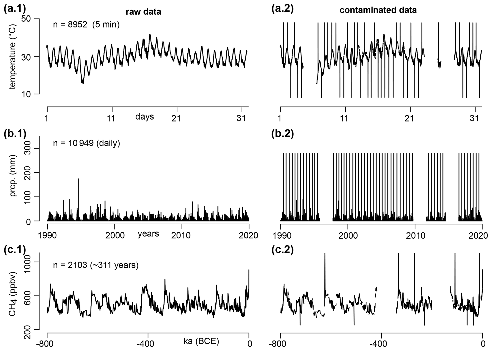
Figure 5 Raw and contaminated versions of the three datasets used as case studies: temperature (a), precipitation (b), and methane (c). The sampling frequency is given in parenthesis. The contaminated versions contain three large data gaps (20 % of the datasets), random missing values (9.5 %), and random outliers (0.5 %) set as a constant level.

3.2.4 Contamination of the datasets

To test for the robustness of the aggregation procedure, the three raw datasets are contaminated by 30 % (Fig. 5, second column) with the use of three data gaps (20 % of the dataset), random NA values (9.5 % of the dataset), and outliers (0.5 % of the dataset). The three data gaps are picked with random length and position. The position of the outliers and the NA values follows a Poisson law. The value of the outliers is picked equal to $y_{\min }-\frac{\mathrm{1}}{\mathrm{2}}(\mathit{\mu }-y_{\min })$ or $y_{\max }+\frac{\mathrm{1}}{\mathrm{2}}(y_{\max }-\mathit{\mu })$, with y_min, y_max and μ respectively the minimum, maximum and mean of the dataset (temperature and methane datasets). The precipitation is supposed to follow a heavy-tail distribution (extremes are more frequent), and negative values are impossible, which is why outlier values are set to 1.6×y_max instead (Supplement).

3.2.5 Aggregation of the datasets

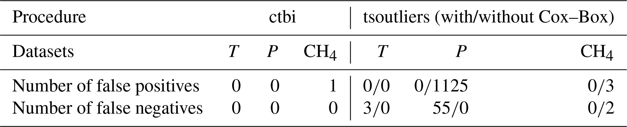
Each dataset (raw and contaminated version) is consecutively aggregated twice (Fig. 6). The temperature dataset is aggregated (using the mean) every hour (n_bin=12) and then every day (n_bin=24). The precipitation dataset is aggregated (using the sum) every month (n_bin=31) and then every year (n_bin=12). The methane dataset is aggregated (using the mean) every 2000 years (n_bin=4) and then every 20 000 years (n_bin=10). For each dataset, the mean cycle of the second level of aggregation is shown in Fig. 6 (second column). The aggregation inputs are chosen as default values. The only exceptions are coeffoutlier=NA and SCI_min=NA for the raw data (outliers are not checked, data are not imputed), f_NA=1 for the methane dataset (bins with at least one non-NA data point are accepted due to the high irregularity in the sampling frequency), and $y_{\lim }=[\mathrm{0},+\mathrm{\infty }[$ for the precipitation dataset (negative precipitation is impossible). The number of false positive (real data points flagged as outliers) and false negative (outliers that have not been flagged) are counted during the first level of aggregation (Table 1), and compared with the tsoutliers function with λ= “auto”, which means that the residuals have been transformed to follow a Gaussian with the Cox–Box method (Box and Cox, 1964), or λ= NULL, which means the original residuals are not transformed. The box plot rule in tsoutliers uses α=3, and the long-term trend or cyclic component are not available for comparison.

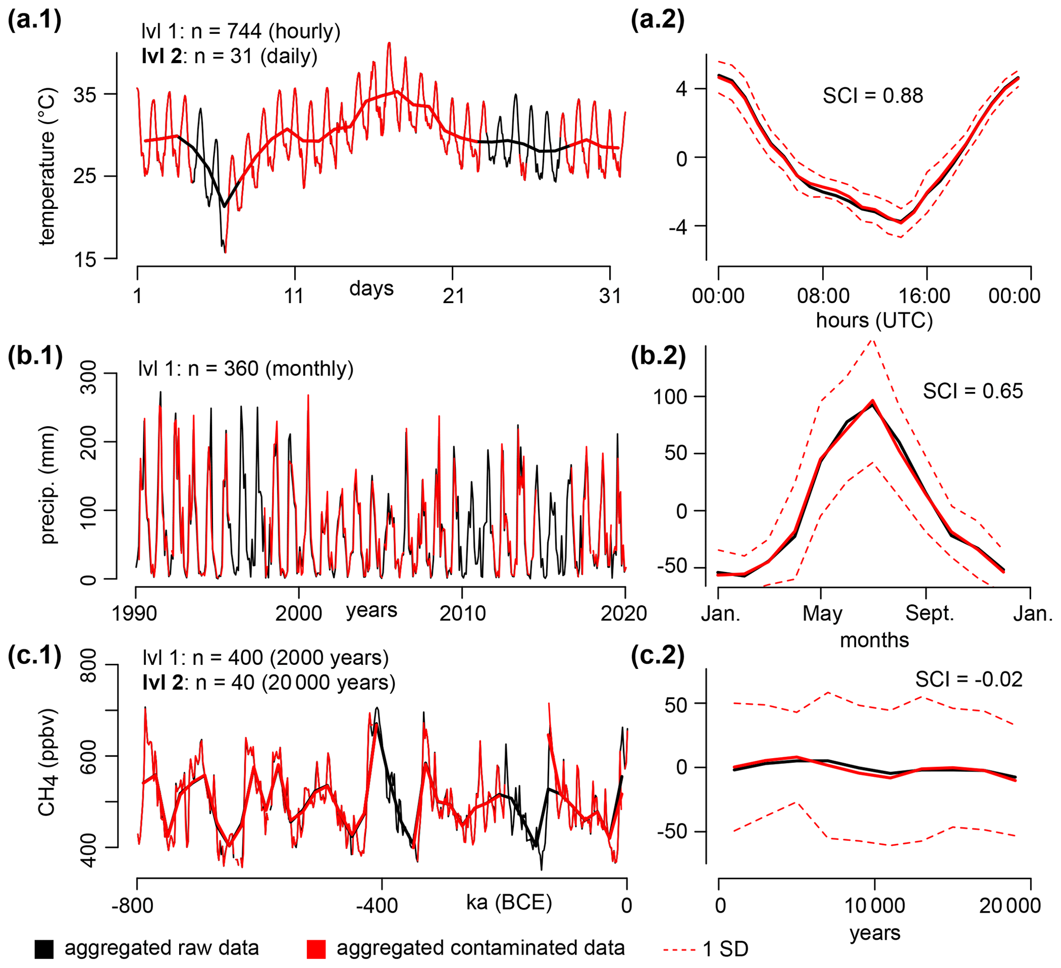
Figure 6 Aggregation of the temperature (a), precipitation (b), and methane (c) in two consecutive levels: 1 (thin lines) and 2 (bold lines). Only the first level of aggregated precipitation is shown for clarity. Black and red colors are associated with the raw and contaminated datasets, respectively. The mean cycles of the second level of aggregation are shown in the second column, with their SCI displayed (the raw and contaminated versions share similar values).

3.3 Results and discussion

The three univariate time series have been chosen as case studies due to their various statistical characteristics that are commonly seen in the scientific or economic field (Fig. 5, 1st column). The long-term trend follows smooth or moderate variations in the temperature and precipitation datasets, but shows a much higher volatility in the methane dataset. The cyclic pattern varies from strong diurnal cycles (temperature) and moderate seasonal cycles (precipitation) to no apparent cyclicity over a period of 20 000 years (methane). The detrended and deseasonalized residuals follow distributions from Gaussian (temperature) or seemingly exponential (methane) to heavy-tailed (precipitation). Finally, the sampling frequency goes from sub-hourly (temperature) or daily (precipitation) to highly variable (1 to 3461 years, methane). To test the limits of the aggregation procedure, these three datasets are severely contaminated by data gaps, outliers, and missing values (Fig. 5, 2nd column).

The first level of aggregation recovers most of the destroyed signal, with ∼80 % of the bins being accepted for all three datasets (Fig. 6). In these accepted bins, all outliers have been correctly flagged (Table 1). The mean percentage of difference between the contaminated and raw aggregates (level 1) is virtually zero for the temperature (0±0.1 %), the methane ($-\mathrm{0.1}\pm \mathrm{2}\mathit{\%}$), and the precipitation (0±17 %). For the methane dataset, the only false positive (Table 1) is located at the beginning of the time series (modern time), because the anthropogenic change in CH₄ is unprecedented when compared to the geological history (the long-term fit does not capture the abrupt increase due to climate change). In comparison, the function tsoutliers successfully flags the outliers in the contaminated temperature and methane datasets (with the Cox–Box method), however it fails with the contaminated daily precipitation dataset (Table 1). This comes from the inability of tsoutliers to handle heavy-tailed distributions, creating 55 false negatives (all outliers have been missed) with the Cox–Box method and 1125 false positives without it, due to the limitation of the box plot rule using a constant α=3 (see part I).

Table 1 Number of false positives (real data points flagged as outliers, type I error) and false negatives (outliers that have not been flagged, type II error) for the contaminated temperature (n=8952), precipitation (n=10 949), and methane (n=2103) datasets shown in Fig. 5, with the ctbi procedure and the tsoutliers function (with/without the Cox–Box method).

The second level of aggregation has been performed to test for the cyclicity in the signal (Fig. 6, 2nd column) using the mean cycles and their associated Stacked Cycles Index (Fig. 4). The raw and contaminated mean cycles share similar magnitude within 1 standard deviation on the mean, and their SCI are the same: −0.02 for the methane (no apparent cycles of 20 000 years period), 0.65 for the precipitation (moderate seasonality), and 0.88 for the temperature (strong diurnal cycles). The SCI reveals itself being useful when comparing signals of different nature or periodicities, which is not possible for seasonal indices that only focus on one field (e.g., hydrology) or data format. (e.g., monthly), such as the seasonality index of Feng et al. (2013). The cyclicity seen in the temperature and precipitation is strong enough to impute the missing data in all accepted bins, which further improves the reconstruction of the signal. Because SCI has a similar structure than a coefficient of determination, imputations based on high SCI (> 0.6) are respecting the original signal, which is sometimes not the case with a linear interpolation. These three case studies demonstrate that ctbi is capable of aggregating signals of poor quality that have a stationary variance in the residuals. The next section explains how to handle more complex time series.

3.4 Limits and recommendations

The ctbi procedure complements the expert knowledge related to a dataset, but it does not replace it. In particular, this procedure is not capable of detecting long periods of instrument failure or human error, and it is essential to flag them manually and/or visually before running ctbi. This procedure also presents difficulties to pre-process signals with a complex seasonality associated with residuals of non-stationary variance. A typical example is a daily precipitation record with a pronounced monsoon: several months of droughts (low variability in the signal) are followed by few weeks of severe floods (high variability). These two periods do not have the same statistical characteristics and need to be treated separately. In this situation, two pools of bins can be created using the MAD as a robust indicator of variability within each bin. The procedure is the following: (i) apply ctbi with the median operator (do not flag outliers or impute data, coeffoutlier=NA, and SCI_min=NA) so that each bin will be associated with a specific MAD; (ii) flag bins with a low MAD (“dry” season) and a high MAD (“wet” season); (iii) split the raw data into two datasets of bins with a low and high MAD, respectively; (iv) apply ctbi separately to each dataset to flag outliers and/or impute data; and (v) merge the two datasets. This procedure is successfully applied to a soil respiration dataset (Supplement).

Other issues can usually be addressed by varying the inputs: period of the bin, maximum ratio of missing values per bin (f_NA), and cyclic imputation level (SCI_min). It is recommended to pick the period of a bin so that it contains on average between 4 and ∼50 data points. Below 4 would decrease the breakdown point to unsafe levels (one outlier would be enough to contaminate the bin) and above 50 would produce a long-term trend that might not properly capture the variability in the signal. A maximum of 20 % of the bin can be missing by default (f_NA=0.2), but when data are sparse and irregularly distributed, a value of f_NA=1 is possible (example with the methane dataset: bins with only one data point were accepted). Finally, the imputation level (default of SCI_min=0.6) can vary between 0 (forced imputation even without cyclic pattern) and 1 (no imputation).

4 Conclusion (part I and II)

Although univariate time series are the simplest type of temporal data, this study reveals a lack of consensus in the literature on how to objectively flag outliers, especially in raw data of poor quality. In part I, a comparison between outlier detection methods is performed on daily residuals from century-old weather stations (precipitation and temperature data). All traditional outlier detection methods flag extreme events as outliers too frequently (type I error). The alternative procedure developed in this study (Logbox) improves the box plot rule by replacing the original α=1.5 with $\mathit{\alpha }=A\log \left(n\right)+B+\frac{\mathrm{36}}{n}$, with A and B determined with a predictor of the maximum tail weight (m_*). Logbox is parameterized on two families of distributions (Pearson and generalized extreme value), and the theoretical percentage of type I error decreases with the sample size ($p_{\mathrm{theo}}=\frac{\mathrm{0.1}}{\sqrt{n}}\mathit{\%}$). Logbox therefore produces cutting thresholds that are tailored to the shape and size of the data, with a good match between observed and expected type I errors in the precipitation and temperature residuals.

In part II, a pre-processing procedure (ctbi for cyclic/trend decomposition using bin interpolation) cleans, decomposes, imputes, and aggregates time series based on data binning. The strength of the cyclic pattern within each bin is assessed with a novel and adimensional index (the Stacked Cycles Index) inspired by the coefficient of determination. The ctbi procedure is able to filter contaminated data by selecting bins with sufficient data points (input: f_NA), which are then cleaned from outliers (input: coeffoutlier). The cyclic pattern within each bin is evaluated (SCI) and missing data are imputed in accepted bins if the cyclicity is strong enough (input: SCI_min). Most of the signal can be retrieved from univariate time series with diverse statistical characteristics, illustrated in this study with a temperature, precipitation, and methane datasets that have been contaminated with gaps and outliers. Limits in the use of ctbi are acknowledged for signals with a long period of instrument failure, but also for signals presenting a complex seasonality. The last situation can be handled by splitting the raw data into two (or more) datasets containing bins with similar variability quantified by the mean absolute deviation (MAD). The pre-processing procedure is then separately applied to each dataset to correctly identify outliers. It is strongly recommended to examine the data before and after using ctbi to ensure that rejected bins and flagged outliers seem reasonable, and to be transparent about the inputs used in your future study.