the Creative Commons Attribution 4.0 License.
the Creative Commons Attribution 4.0 License.
 | 27 Sep 2023
Drought intensity–duration–frequency curves based on deficit in precipitation and streamflow for water resources management
Yonca Cavus
Kerstin Stahl
Hafzullah Aksoy
Drought estimates in terms of physically measurable variables such as precipitation deficit or streamflow deficit are key knowledge for an effective water management. How these deficits vary with the drought event severity indicated by commonly used standardized indices is often unclear. Drought severity calculated from the drought index does not necessarily correspond to the same amount of deficit in precipitation or streamflow at different regions, and it is different for each month in the same region. We investigate drought to remove this disadvantage of the index-based drought intensity–duration–frequency (IDF) curves and develop IDF curves in terms of the associated deficit. In order to study the variation of deficits, we use the link between precipitation and streamflow and the associated indices, the Standardized Precipitation Index (SPI) and the Standardized Streamflow Index (SSI). More specifically, the analysis relies on frequency analysis combined with the total probability theorem applied to the critical drought severity. The critical drought has varying durations, and it is extracted from dry periods. IDF curves in terms of precipitation and streamflow deficits for the most severe drought of each drought duration in each year are then subject to comparison of statistical characteristics of droughts for different return periods. Precipitation and streamflow data from two catchments, the Seyhan River (Türkiye) and the Kocher River (Germany), provide examples for two climatically and hydrologically different cases. A comparison of the two cases allows a similar method to be tested in different hydrological conditions. We found that precipitation and streamflow deficits vary systematically, reflecting seasonality and the magnitude of precipitation and streamflow characteristics of the catchments. Deficits change from one month to another at a given station. Higher precipitation deficits were observed in winter months compared to summer months. Additionally, we assessed observed past major droughts experienced in both catchments on the IDF curves, which show that the major droughts have return periods at the order of 100 years at short durations. This coincides with the observation in the catchments and shows the applicability of the IDF curves. The IDF curves can be considered a tool for using in a range of specific activities of agriculture, ecology, industry, energy and water supply, etc. This is particularly important to end users and decision-makers to act against the drought quickly and precisely in a more physically understandable manner.
- Article
(8970 KB) - Full-text XML
- BibTeX
- EndNote


The risk of climate extremes has increased with global change and presents great challenges to the management of unprecedented droughts (Kreibich et al., 2022). Therefore, reliable drought analyses and estimations are needed to protect people's water demand in a sustainable way by mitigating the effect of water scarcity. Drought has been commonly assessed by using different types of standardized drought indices. These drought indices are derived from different variables each representing different types of droughts such as precipitation for meteorological drought, soil moisture for agricultural drought and streamflow for hydrological drought. Standardized drought indices are used by national meteorological and hydrological services around the world due to their advantage of being non-dimensional variables, and they are useful for comparison of drought in different climate regions in terms of their characteristics such as duration, intensity, severity and return period. The separate use of the duration, severity/intensity and return period is not sufficient for a comprehensive drought characterization unless they are related in the form of severity/intensity–duration–frequency (S/IDF) curves. IDF curves reflect the statistical characteristics of variables and the relation among intensity and frequency for different durations at a station, providing rich hydrological information in a single graph. Similar to precipitation IDF curves which are traditionally used in hydrological design, this study concentrates on drought IDF curves which can be proposed as useful tools in water management against low extremes.
Studies on the drought S/IDF curves are limited in the drought literature. In the existing literature, drought S/IDF curves have been developed mainly by using drought indices. As an early study, Dalezios et al. (2000) developed drought SDF curves based on the Palmer drought severity index in the form of tables and isolines illustrating more severe droughts for longer return periods. Drought severity and duration were combined by a probabilistic model, and copulas were applied on the Standardized Precipitation Index (SPI) to construct the joint distribution function and to establish the drought SDF curve in the form of return period isolines (Shiau and Modarres, 2009). In addition, performances of different copulas using various statistical methods were tested for the derivation of drought SDF curves based on the SPI (Reddy and Ganguli, 2012). Todisco et al. (2013) developed index-based SDF curves and integrated them with a methodology to account for the economic impact of drought. Halwatura et al. (2015) derived SDF curves at different timescales by using bivariate functions of duration and severity calculated from several drought indices. Most recently, Aksoy et al. (2021) focused on IDF curves of critical droughts based on the SPI by using an empirical relationship between the drought intensity and its return period.
The drought curves described above are non-dimensional IDF or SDF curves based on standardized drought indices to assess drought characteristics as in a few more studies (Gupta et al., 2020; Sahana et al., 2020; Pandya and Gontia, 2023). To date, only a few studies have investigated drought S/IDF curves and their relation with physical drought indicators such as soil moisture, runoff, precipitation deficit and streamflow deficit, limiting the experience to a few specific regions. For example, Sung and Chung (2014) developed dimensional-drought SDF curves based on streamflow deficit using various threshold levels for water use in South Korea. These drought S/IDF curves presented an insight into the use of deficits for a humid continental climate. Cavus and Aksoy (2020) presented station-based S/IDF curves to quantify the recurrence intervals of critical droughts based on precipitation deficit for the Mediterranean climate.
We know that the same value of a drought index corresponds to different deficits in different regions. Meteorological and hydrological droughts correspond to temporal anomalies changing also spatially from one catchment to another, and they are characterized based on long-term conditions, which are related to climatic and environmental factors (Vicente-Serrano et al., 2013; van Loon, 2015). Therefore, the same value of a drought index corresponds to different deficits in different regions. The non-dimensionality of drought indices comes at the expense of physical non-interpretability; i.e., most drought indices cannot be read quantitatively as actual precipitation and streamflow deficits. In climates with high seasonal variation (i.e., Mediterranean climate), the difference between deficits varies greatly each month, while this difference may be lower in regions with low seasonality (i.e., humid climate). Determination of precipitation and streamflow deficits is a challenge when common drought indices are used. Thus, any non-dimensional drought severity or intensity derived from index series might insufficiently represent the actual water availability for water management under drought conditions. In practice, deficits under drought conditions in different climates and catchments need to be quantified and be linked with the duration, deficit volume and return periods. With SDF or IDF curves we can construct this relation to quantify drought characteristics and obtain knowledge about past drought events for practical consideration, which is the motivation of this study to derive deficit-IDF curves.
The overarching objective is to develop drought IDF curves based on precipitation and streamflow deficits at different timescales and appraise their usefulness in different climates. For this, drought index-derived characteristics are converted into precipitation and streamflow deficits for different cases. For comparison, two catchments are considered in different climatic regions. Hence, the comparison between the regions and among the variables provides the framework of analysis. Specifically, we aim to assess how the deficits vary in the considered study regions and finally explore how deficit-IDF curves might be used for different purposes. The study addresses the following research questions:
-
How different are deficit-IDF curves from their non-dimensional index-based counterparts?
-
What is the relation between drought indices and indicators? How do deficits in precipitation and streamflow change with the associated standardized drought index in time and space?
-
For what purposes might deficit-IDF curves be used in water management practice?
Table 1Characteristics of selected meteorological and streamflow gauging stations in the Seyhan (Türkiye) and the Kocher (Germany).
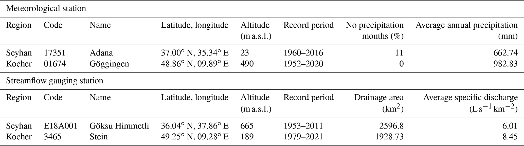
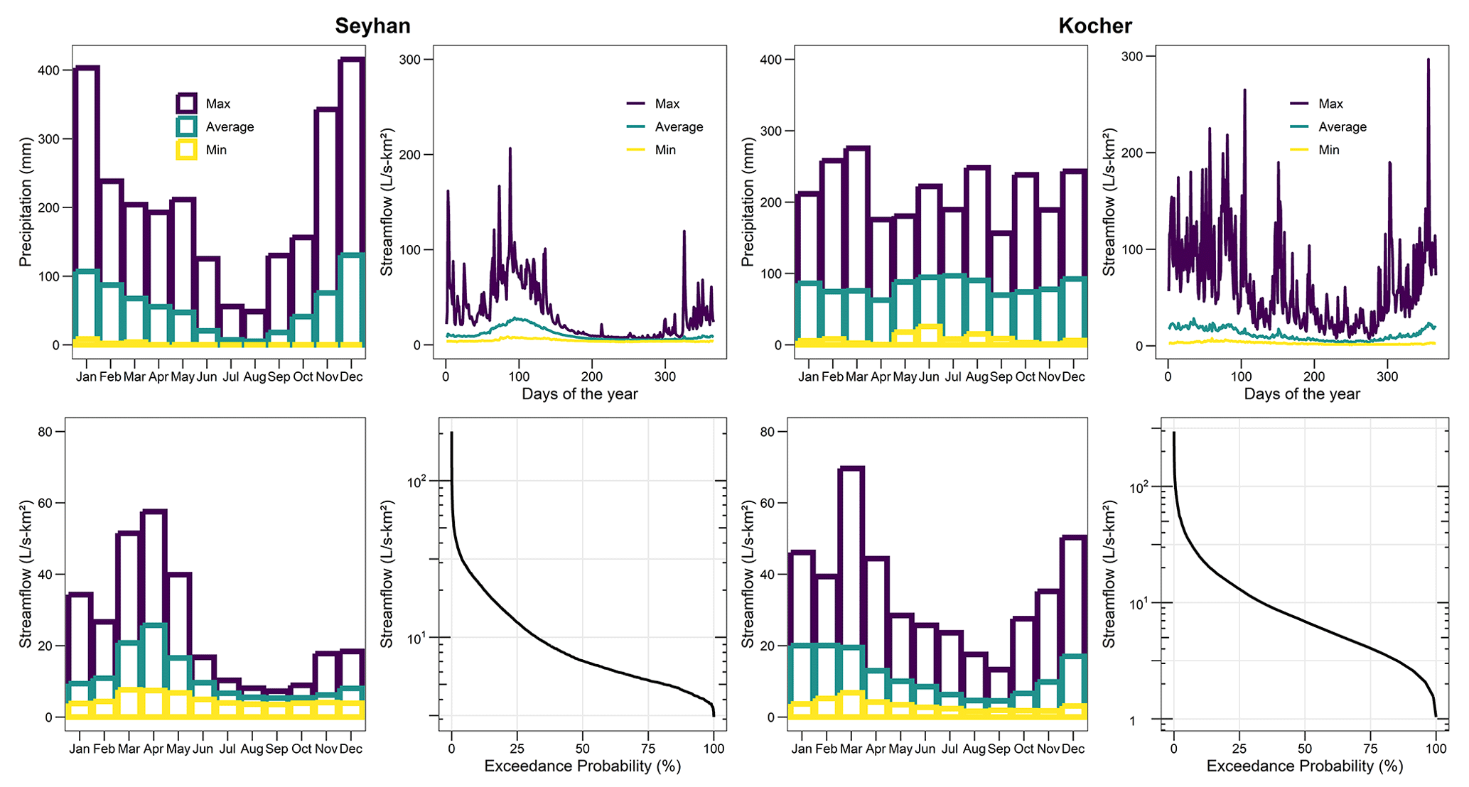
Figure 1Seasonal characteristics of the meteorology and streamflow gauging stations with their flow duration curves for Seyhan and Kocher.
Precipitation and streamflow data from meteorological and streamflow gauging stations of two regions, one in Türkiye and another in Germany, were used. We selected the Seyhan River basin in southern Türkiye and the Kocher catchment in southwestern Germany. Seyhan River is important for the production of hydroelectric energy and the basin itself for irrigated agricultural activities, which increases water demand under low water availability (GDWM, 2019). The Kocher River is important for agricultural activity and hydropower production from run-of-the-river power plants (Zeitler et al., 2017).
The selected gauging stations from the headwaters of these basins are a subset of the benchmark catchments with good hydrometric performance and nearly natural flow conditions. The selected stations have a long-record-length dataset, which is crucial for correctly characterizing the drought and estimating the long-return-period droughts (Table 1). The data of the selected catchments come from various sources. For Türkiye, monthly precipitation data of station-based observation come from the State Meteorological Service (MGM). Daily streamflow data were downloaded from the State Hydraulic Works (DSI) website. For Germany, daily precipitation data were downloaded from the climate data center of the German Weather Service (DWD) website. Streamflow data of this catchment were acquired from the Environment Agency of Baden-Württemberg (LUBW).
The seasonality in precipitation and streamflow of Seyhan follows a typical Mediterranean climate with a wet winter and a dry summer. It produces seasonal precipitation and streamflow variation with peaks in December and April, respectively, and a low precipitation and flow period extending over the summer (Fig. 1). The seasonality of precipitation in the Kocher catchment varies over the year with higher precipitation in winter and summer and less precipitation in spring and autumn. Streamflow varies within the year, with high flows in winter and low flows in summer. Flow duration curves (FDCs) show the Kocher can sustain flow longer, and then it decreases sharply at the lower end, while the Seyhan gradually approaches the minimum. This is a distinct difference in the important lower part of the FDCs. In the long-term average daily streamflow in the Seyhan, maximum values concentrated in winter. In the Kocher, high flows are likely to be observed throughout the year, except for a period from July to September. However, in this period, maximum values are still higher than the long-term average of the daily streamflow.
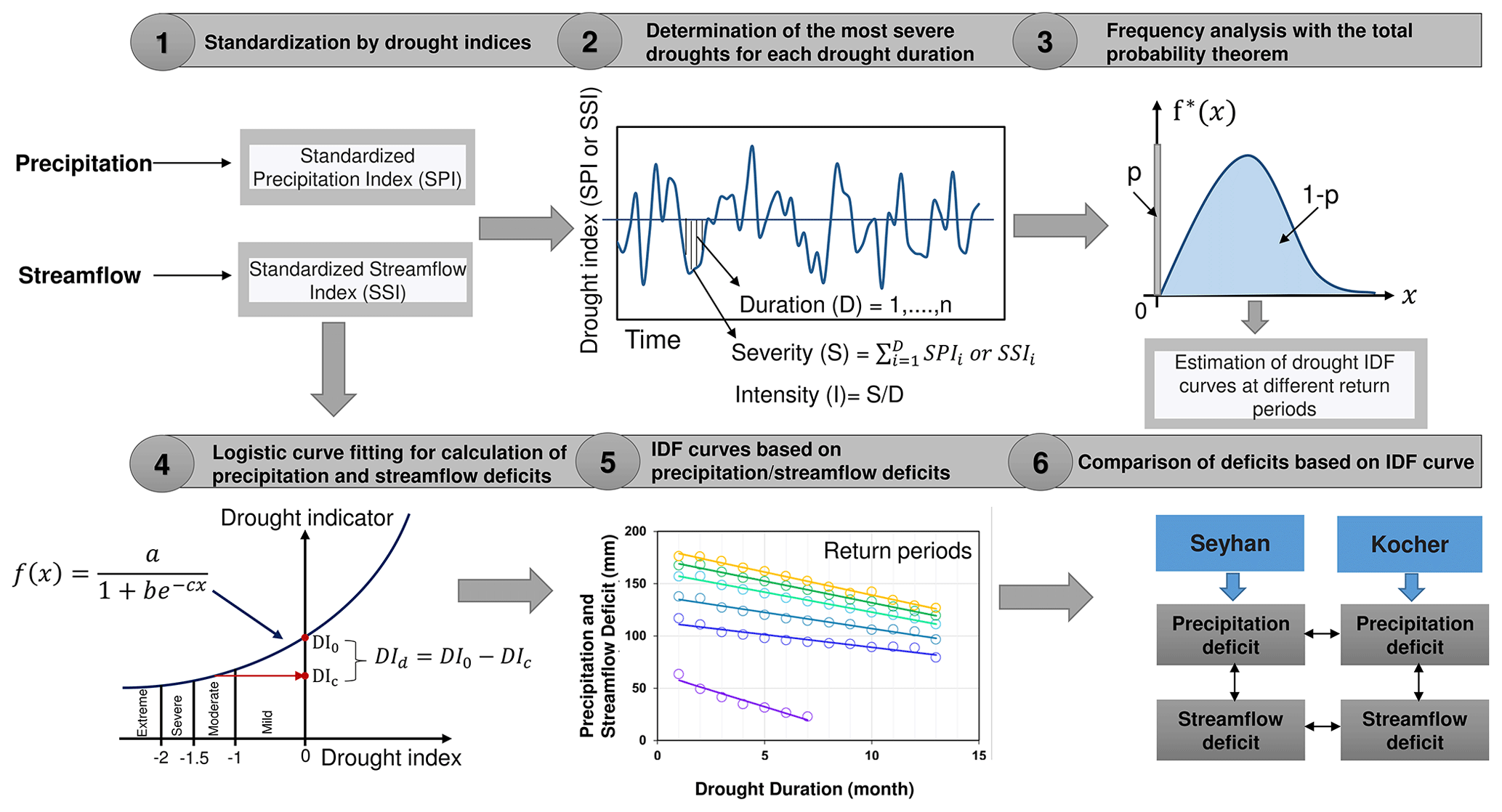
Figure 2Illustration of the methodology used to develop drought IDF curves based on precipitation deficit and streamflow deficit.
This study follows several methodological steps (Fig. 2): (1) calculation of standardized drought indices, (2) determination of the most severe (critical) droughts for each drought duration, (3) application of frequency analysis with the total probability theorem to critical drought severity, (4) calculation of precipitation and streamflow deficits by using logistic curve fitting, (5) derivation of drought IDF curves based on precipitation/streamflow deficits and (6) comparative analysis of IDF curves.
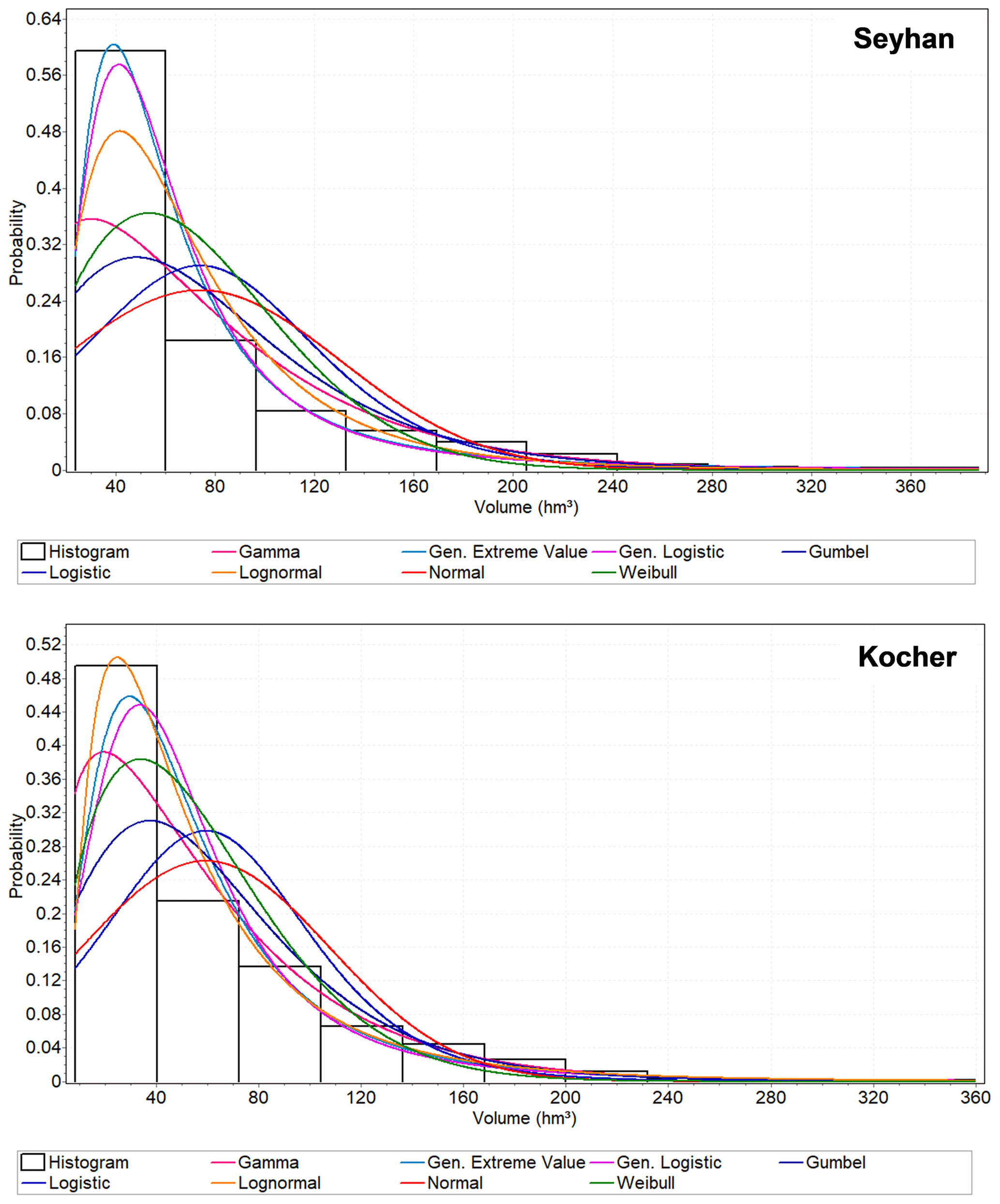
Figure 3Probability distribution functions fitted to streamflow volume for selected gauging stations in the Seyhan River basin and the Kocher catchment.
Step 1 involves standardization by drought indices. To characterize the drought, we used the Standardized Precipitation Index (SPI; McKee et al., 1993) and the Standardized Streamflow Index (SSI; Vicente-Serrano et al., 2012) (Fig. 2). They are well-established drought indices which are widely used for the drought quantification. The SPI was calculated using monthly precipitation data accumulated at 1-, 3-, 6- and 12-month timescales. Similarly, SSI time series of the same timescales were calculated to detect the total aggregated streamflow deficit. Precipitation was used as the monthly total precipitation for the SPI, while streamflow was taken as the volume of monthly average streamflow for the SSI. The gamma probability distribution function is fitted to the precipitation data and transformed to the standard normal distribution with zero mean and unit standard deviation (McKee et al., 1993). Based on the Anderson–Darling statistical test of several probability distribution functions including gamma, generalized logistic, generalized extreme value (GEV), Gumbel, logistic, lognormal, normal and Weibull, we found the GEV distribution to be the best and LN2 the second best for the Seyhan and LN2 the best and GEV the second best for the Kocher for the streamflow volume accumulated over a month (Fig. 3). The length of the streamflow record and the selected probability distribution function strongly affect the calculated SSI (Wu et al., 2005, Tijdeman et al., 2020). To allow a comparison of the streamflow deficits in the two different case study rivers in different climate regions, here we used GEV for both catchments for comparability reasons and also to be in accordance with the literature (Vicente-Serrano et al., 2012).
In Step 2, dry periods were identified from the SPI and SSI time series (Fig. 2). Any period of time with SPI and SSI values lower than zero (SPI < 0 or SSI < 0) was considered a dry period. Based on the concepts of Cavus and Aksoy (2020), dry periods consist of droughts; a dry period has a fixed length and a drought has a duration. Drought duration changes from 1 month to the dry-period length. A drought with duration shorter than the dry-period length is a within-period drought, and a drought with duration that covers the whole dry-period length is a singular drought. The sum of consecutive negative values of the drought index for each drought duration is the drought severity. The drought intensity is the drought severity divided by the drought duration. In any year, drought of a given duration with maximum severity was taken as the critical drought for each particular duration. When only one drought exists within 1 year, no matter how long and how severe it is, we assigned it as the critical drought to this particular year. A year in which drought is not observed is called the no-drought year, and for such a year, the critical drought severity is zero. For further definitions and explanations of these drought concepts, see Cavus and Aksoy (2019, 2020) and Aksoy et al. (2021).
In Step 3, frequency analysis was applied on the critical drought severity of each duration at each timescale (Fig. 2). In no-drought years, the critical drought severity is zero as these years are totally covered by a wet period. Thus, the critical drought severity time series has zero and non-zero values. Frequency analysis was applied on non-zero critical drought severity time series with a minimum of 10 years from which zero values were removed. Zero values in the drought severity time series have a probability of occurrence, while the non-zero values have a probability distribution function. The total probability theorem described in the literature (Haan, 1977, Aksoy et al., 2021) was applied to datasets with zero and non-zero values. The best-fit probability distribution function of the non-zero critical drought severity was determined by taking into account the occurrence probability of zero values. We considered the two- and three-parameter gamma (G2, G3), the generalized extreme value (GEV), the two- and three-parameter log-normal (LN2, LN3), log-Pearson type 3 (LP3), and the two- and three-parameter Weibull (W2, W3) probability distribution functions, which are widely used in the literature. We used absolute values of the critical drought severity in the frequency analysis as the probability distribution functions are only expressed for positive variables. We decided on the best-fit probability distribution function after the Anderson–Darling statistical test. The critical drought severities corresponding to 2-, 5-, 10-, 25-, 50- and 100-year return periods were calculated for all drought durations by using the fitted probability distribution function of the relevant drought duration.
As the SPI and SSI are calculated from precipitation and streamflow, respectively, a strong relationship can be expected between the drought indicators (precipitation and streamflow) and the associated drought indices (SPI and SSI). This relationship is determined in Step 4 by applying curve fitting in the form of nonlinear regression (Fig. 2). To establish a functional relationship between the drought indicators and the drought indices, we tested several curves including the second- and third-order polynomials and exponential, Gompertz and logistic curves. The polynomials and exponential and Gompertz curves were discarded as they produced negative values of precipitation or streamflow, and they could not fit properly to SPI or SSI time series. The logistic curve was selected as the best-fit curve because it provided the highest correlation without producing negative precipitation and streamflow values (Sit and Poulin-Costello, 1994). The logistic function is given by
in which x is the drought index, and a, b and c are parameters. Each month in the time series has a drought indicator (precipitation or streamflow) accumulated at 1-, 3-, 6- and 12-month timescales and the corresponding drought index (SPI or SSI) at the same timescales. Regression equations were developed between the drought indicators and indices by using their all values. Owing to periodicity (seasonality), the relation changes from month to month for timescales shorter than a year; 12 regression equations were obtained for 1-, 3- and 6-month timescales, and one regression equation was obtained for the 12-month timescale.
In Step 5, drought indices were converted to precipitation and streamflow deficits by using the relation between the drought indicators and indices. The critical drought severity corresponding to each drought duration and return period were inserted into the generalized logistic function (Eq. 1) to find the critical precipitation or critical streamflow value (DIc). The precipitation or streamflow value corresponding to the maximum drought severity was calculated from the logistic function. We consider SPI = 0 and SSI = 0 as the threshold value of the drought index for all timescales. Threshold values of drought indices were inserted into the logistic function to calculate the threshold drought indicator (DI0). The difference between the threshold drought indicator and the critical drought severity is deficit in the drought indicator (DId), which is either precipitation deficit or streamflow deficit. For each duration and return period, it is calculated by
Based on the calculated precipitation and streamflow deficits, drought IDF curves of the meteorological and streamflow gauging stations were plotted at different timescales. These deficits provide knowledge to quantify drought IDF curves in terms of physical variables, which are the precipitation deficit and streamflow deficit.
Finally, in Step 6, drought IDF curves are compared between precipitation and streamflow deficits to determine how precipitation deficit propagates to streamflow deficit in these two catchments and how the deficits change from one catchment to another. Additionally, for the assessment of the applicability of the deficit-IDF curves we evaluated one specific drought event observed in each catchment. A severe drought hit the Eastern Mediterranean in 2008, particularly its southern part where the Seyhan River basin is located (GDWM, 2019; Cavus et al., 2022). The Kocher catchment was affected by the drought event of 2018 in central Europe (Brunner et al., 2019; Tijdeman et al., 2022; Rakovec et al., 2022). To show the characteristics of these major droughts on the deficit-IDF curves, we identified months with the highest severity accumulated over 12 months for droughts of different durations from D = 1 month to the longest duration in the IDF curves. We considered the 12-month-timescale IDF curves for this demonstration. For each duration, the precipitation deficit was calculated by taking the difference between the 12-month precipitation accumulation and precipitation threshold of the precipitation record. The largest value of precipitation deficits calculated as the critical value of each duration was then replaced on the deficit-IDF curves to derive the return period of the observed drought.
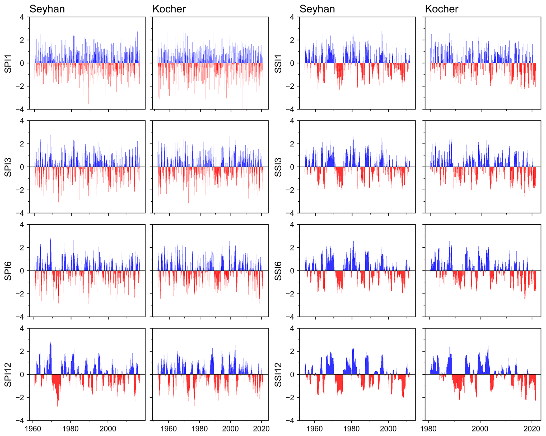
Figure 4The SPI and SSI time series at 1-, 3-, 6- and 12-month timescales for Seyhan and Kocher.
4.1 Drought indices and indicators
The time series of the SPI show a high variability with frequent fluctuations at shorter timescales. At longer timescales, the time series become smoother with fewer fluctuations (Fig. 4). At the meteorological station in the Seyhan basin, dry periods become more visible with increasing timescale at the beginning of the time series. A similar observation can be made for the Kocher catchment. SPI time series at Kocher show lower negative values than those at Seyhan. Higher variability and more frequent fluctuations are also evident in the SSI time series at short timescales, while they become smoother with lower variability and less frequent extreme values at longer timescales (Fig. 4). However, the SSI time series fluctuates less frequently compared to the SPI time series. Major dry periods in the Seyhan are visible in 1974, 1990, 2008 and 2014 in the SPI and SSI time series, particularly when the timescale increases. Drought events in the Kocher catchment are visible in 1990 and 2018 in the SPI and SSI time series.
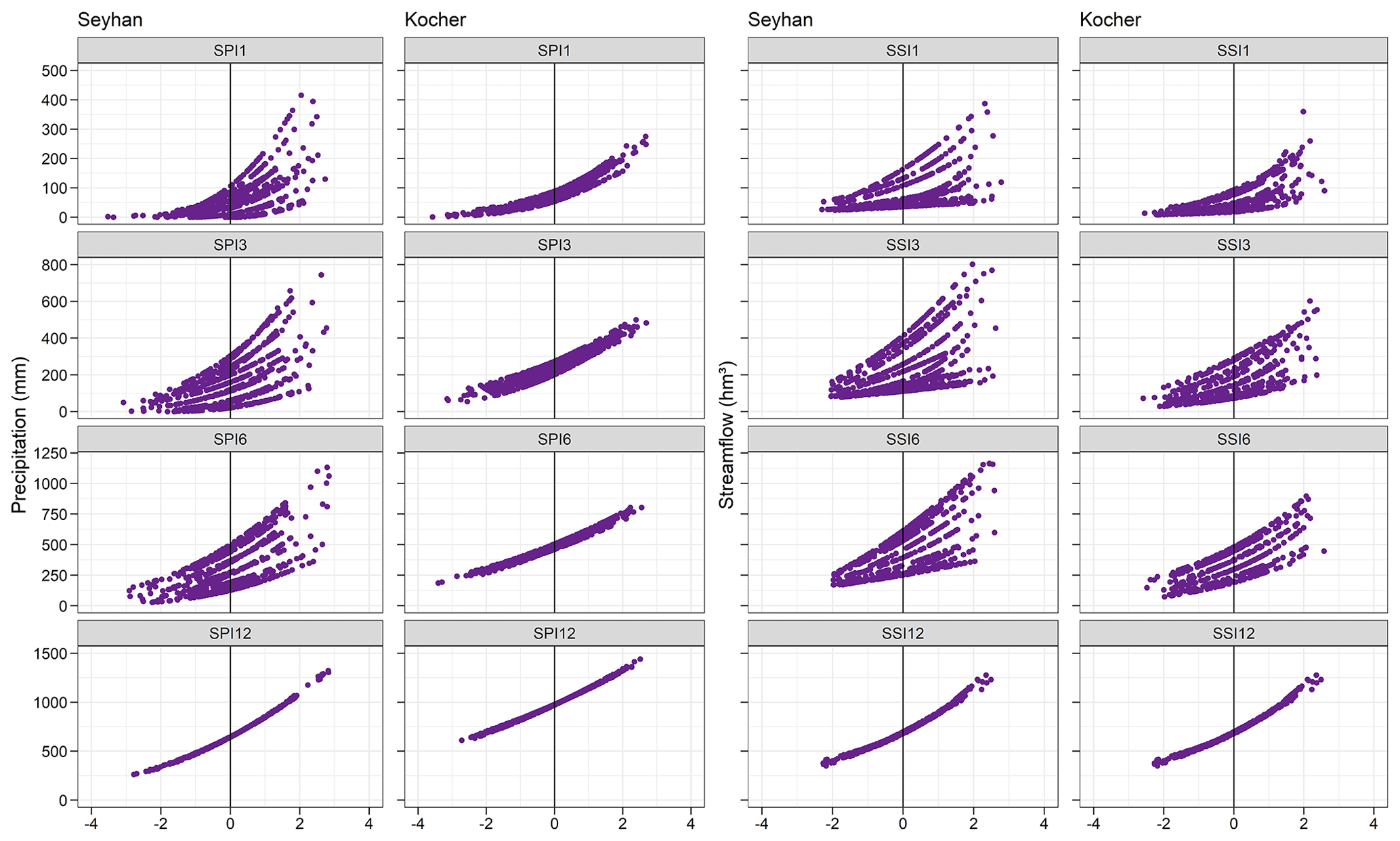
Figure 5The relation between precipitation as a drought indicator and the SPI and precipitation as a drought indicator and the SSI at 1-, 3-, 6- and 12-month timescales for the Seyhan and Kocher. The horizontal axis indicates SPI and SSI values at the top of each scatter diagram.
The previously described seasonality in general precipitation (Sect. 2) is also evident in the relation between precipitation and the drought index, the SPI, at 1-, 3- and 6-month timescales, for which 12 curves were obtained (Fig. 5). At the annual timescale, the relation between precipitation and the SPI is represented by one a single curve as the annual precipitation has no seasonality. In comparison, the precipitation seasonality in the Kocher is not as dominant as that in the Seyhan, and it becomes less pronounced with increase in the timescale. Therefore, at the 1-, 3- and 6-month timescales, monthly curves between precipitation and the SPI are less variable due to less seasonal precipitation in the Kocher than the Seyhan. Because of the climate characteristics (given by the base climatology), the derived drought characteristics differ. Similar to the case for precipitation, Fig. 5 clearly shows that the relation between streamflow and SSI changes from month to month at timescales of 1, 3 and 6 months due to the within-year seasonality of streamflow. Therefore, separate equations of each month should be used at sub-annual timescales. One equation can be used for the 12-month timescale as the seasonality in the streamflow is removed at the annual scale. The variability in the curves that were fitted to obtain the relation between streamflow and the SSI shows the seasonality in the streamflow of the Kocher catchment, although it is still less compared to the variability in the curves of the Seyhan.
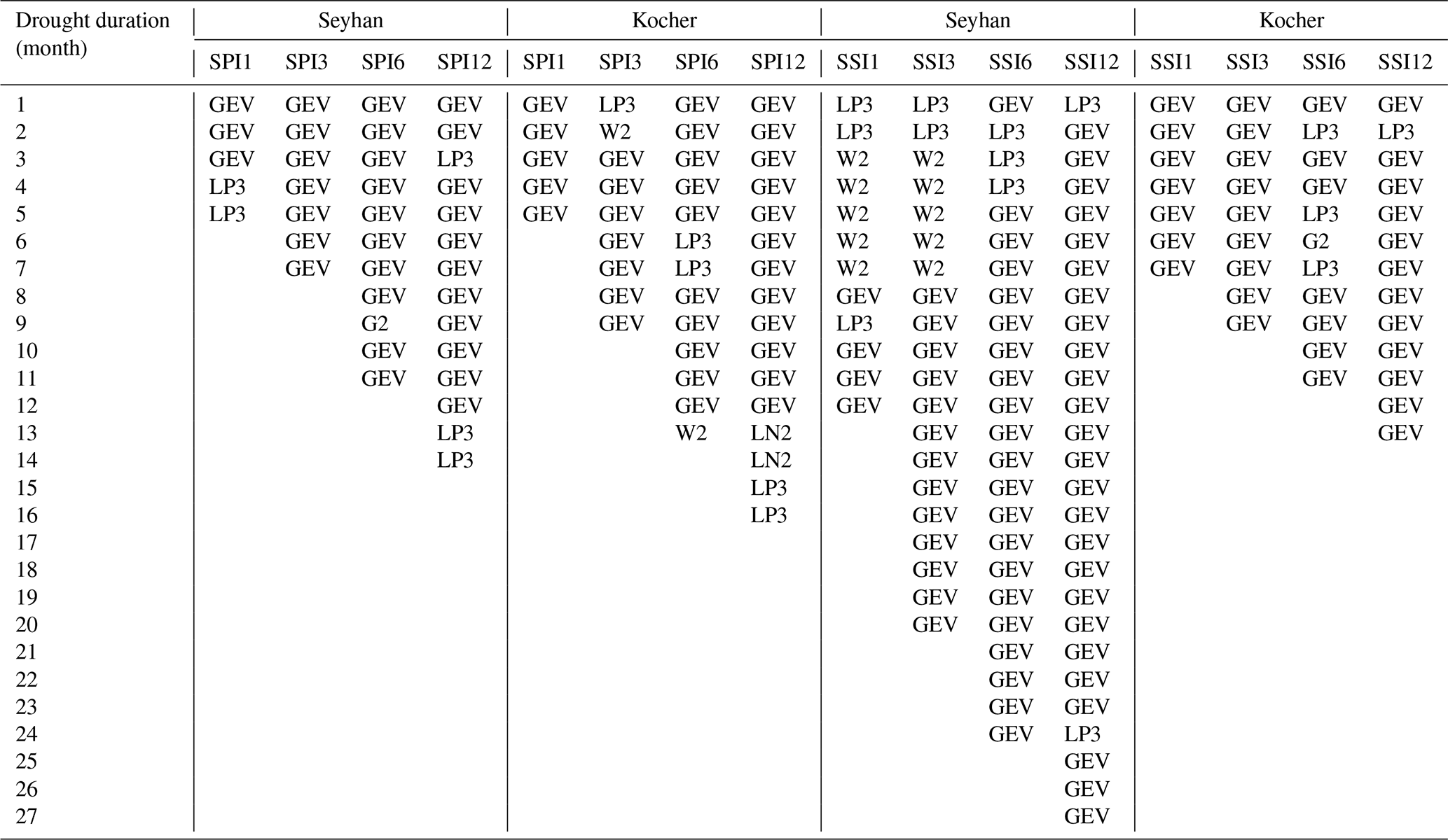
Table 2The best-fit probability distribution functions of the critical drought intensities of different durations for the timescales used.
4.2 Frequency analysis of critical drought severity
Frequency analysis of the critical drought severity shows that GEV is the best-fit probability distribution function for the majority of cases when all droughts at all the timescales are considered in the meteorological and hydrological data records (Table 2). The LP3, W2, LN2 and G2 distributions can be considered as alternative distributions for a few cases among which LP3 is the second-best distribution for the critical drought severities calculated from SPI12 in both catchments. At this particular timescale of the SPI, the best-fit probability distribution function tends to change from GEV to an alternative probability distribution function for long drought durations.
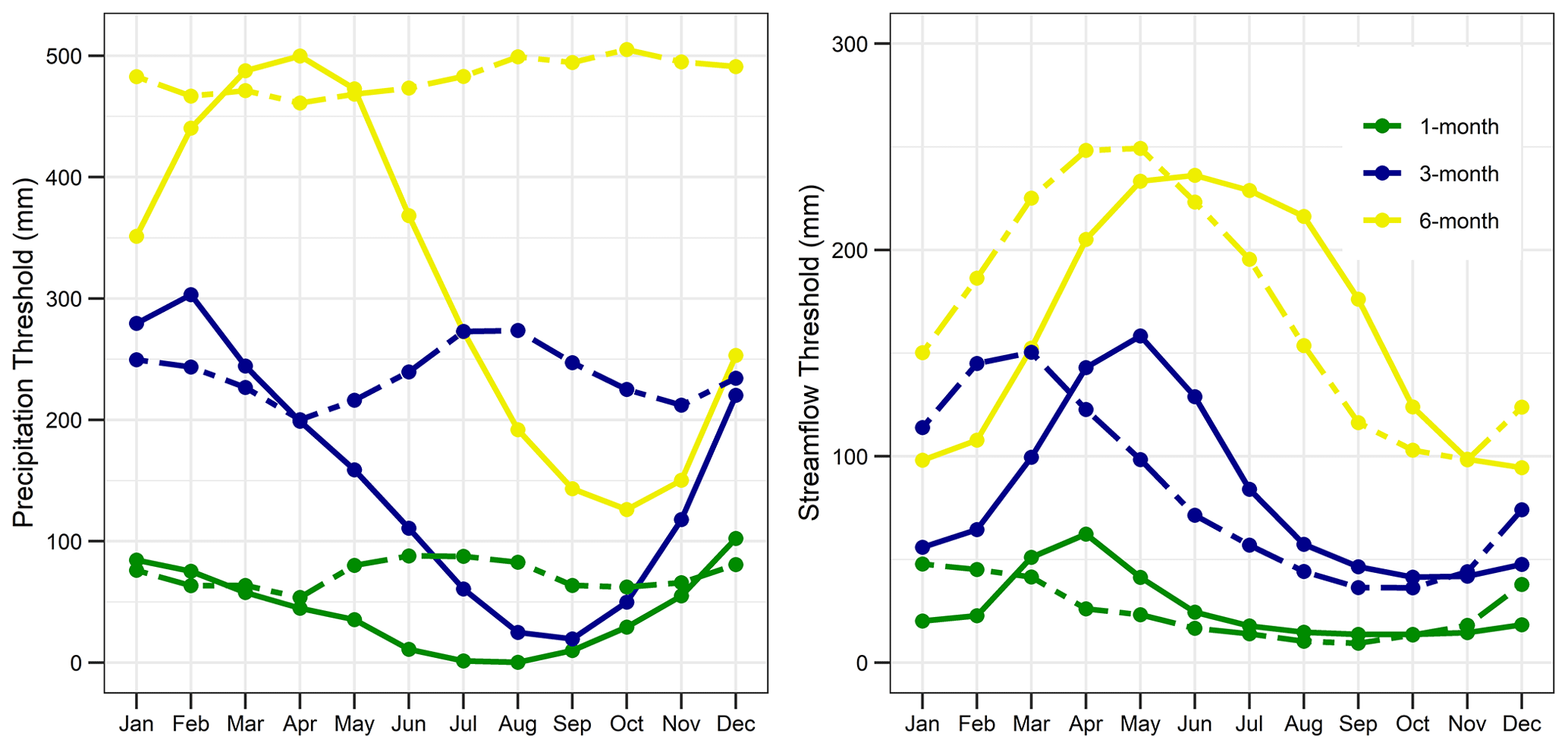
Figure 6Precipitation threshold and streamflow threshold corresponding to SPIk = 0 and SSIk = 0 (k=1, 3, 6 months). Solid lines are for Seyhan and dashed lines for Kocher. The 12-month thresholds are constant values over the year; PTH = 643.88 mm and STH = 333.39 mm for Seyhan and PTH = 975.57 mm and STH = 356.18 mm for Kocher.
4.3 Deficit-IDF curves
Precipitation and streamflow thresholds are needed to calculate deficits in precipitation and streamflow, the key elements of the deficit-IDF curves. The thresholds are not constant over the year at 1-, 3- and 6-month timescales (Fig. 6). They change from one month to another, and also the value of the thresholds changes notably from precipitation to streamflow. The annual thresholds are constant values as they accumulate the within-year seasonality. The clear seasonal variability of precipitation threshold in the Seyhan is not evident in the Kocher, while the streamflow threshold has a notable seasonality in both catchments. These temporal and spatial variabilities in the thresholds prevent the drought IDF curves from being comparable in time and space. For the sake of comparability of the IDF curves of various timescales at two different catchments, precipitation deficit and streamflow deficit were divided by the respective precipitation threshold (PTH) and streamflow threshold (STH), respectively.
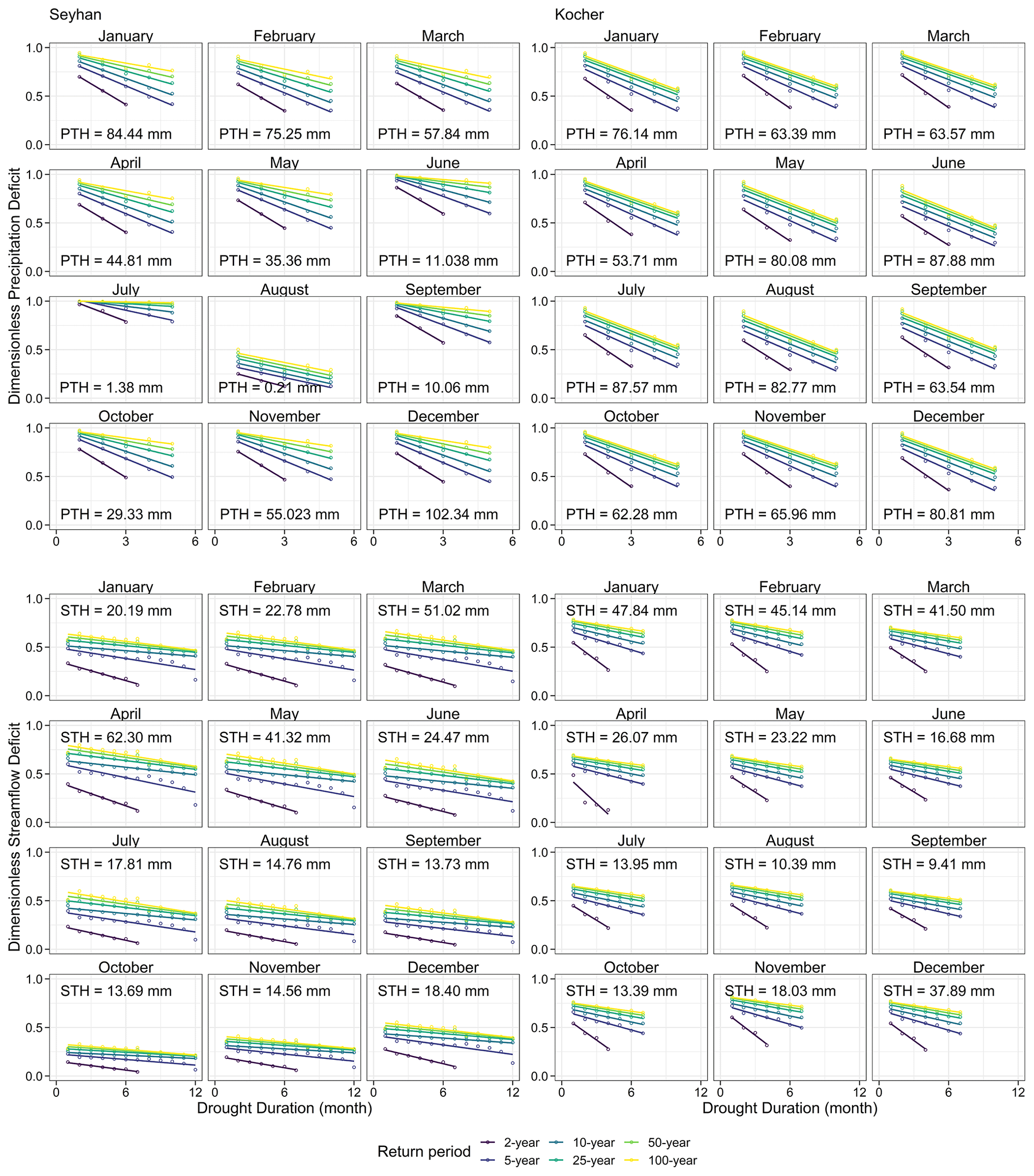
Figure 7Drought IDF curves in terms of precipitation and streamflow deficit divided by the threshold value for the Seyhan and Kocher at a 1-month timescale.
Drought IDF curves of precipitation and streamflow deficits are presented for each month separately at 1-, 3-, and 6-month timescales (Figs. 7, A1 and A2), while the annual deficits are presented in one single set of IDF curves (Fig. A3). Drought IDF curves of precipitation and streamflow deficits show general similarities in the two different climatic regions. In all IDF curves, the precipitation and streamflow deficits decrease linearly as the drought duration increases. The IDF curves are almost parallel to each other for return periods of 5 years and higher. Deficits at the 2-year return period decrease faster; they are therefore separated from other return periods. However, the 2-year return period shows a steeper decrease rate of streamflow deficit in the Kocher than in the Seyhan and a relatively steeper decrease than the curves for higher return periods. Compared to the precipitation and streamflow thresholds, droughts in precipitation are more intense than in streamflow. In addition, precipitation deficits in summer are less in absolute values than in winter considering the seasonality in the precipitation threshold with higher values in winter than summer. Precipitation deficits are particularly lower during the summer months than the winter months in the Seyhan because of the dominant seasonality in the Mediterranean climate, while no notable difference was observed between precipitation deficits in summer and winter in the Kocher because of the negligible seasonality in precipitation in the humid climate of this catchment. The linear decrease in deficits with increasing drought duration and the faster decay in the 2-year return period for the 3-, 6- and 12-month timescales (Figs. A1–A3) are similar to what we obtained at the 1-month timescale (Fig. 7).
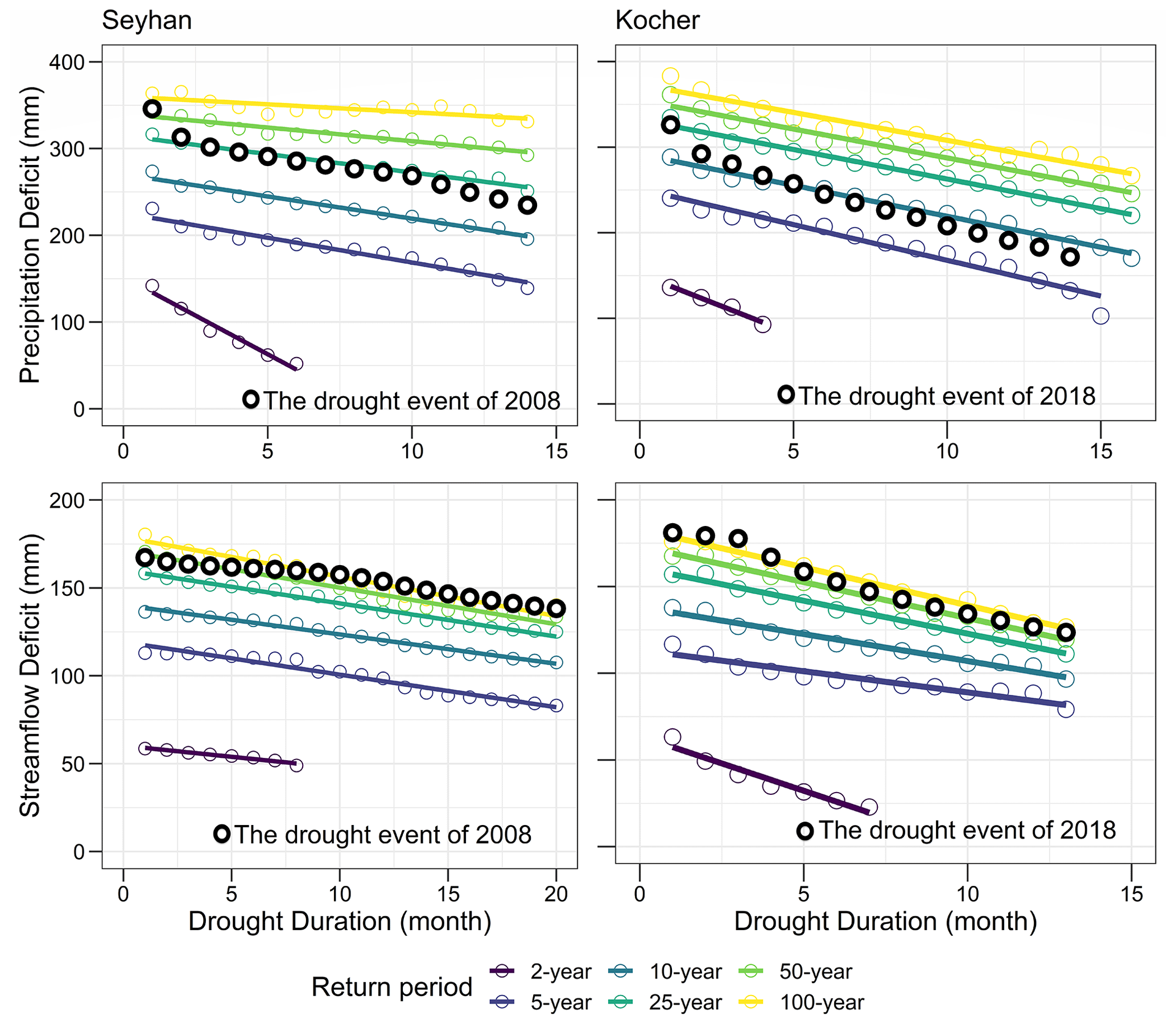
Figure 8Drought IDF curves in terms of precipitation and streamflow deficits at a 12-month timescale. The drought events of 2008 in the Seyhan River basin and 2018 in the Kocher catchment were used to demonstrate the applicability of IDF curves.
4.4 Observed major droughts in deficit-IDF curves
The applicability of the drought IDF curves was tested for two specific drought events; the drought of 2008 in the Seyhan River basin and the drought of 2018 in the Kocher catchment. By selecting the most critical drought of each duration, the observed drought events were plotted onto the drought IDF curves at the 12-month timescale (Fig. 8). In the drought events, precipitation and streamflow deficits decrease as the drought duration increases. The precipitation deficit of the drought event in the Seyhan corresponds to an event with about a 50-year return period at 1-month drought duration and around a 25-year return period at longer durations. The return period declines with increase in the drought duration. However, streamflow deficit exceeds the 50-year return period in the most critical month. The drought in the Kocher was a 25-year event at short durations and a 10-year event at longer durations in terms of precipitation deficit. Streamflow deficit-IDF curves' relations of intensity, duration and frequency are generally similar to precipitation deficit curves. The drought event of 2018–2019 in Kocher streamflow had a return period higher than the 100-year return period for durations shorter than 4 months and higher than the 50-year return period for longer durations. In both cases, the selected drought events approach the 100-year return period. In general, deficit in precipitation of a given return period is higher than streamflow deficit.
5.1 Drought IDF curves for deficit indicators
We extended earlier studies on drought index (DI)-based IDF curves showing drought characteristics of a station in one single graph (Aksoy et al., 2021) to deficit-based monthly IDF curves. Based on those, this work first aimed to explore the question of how these new curves relate to their non-dimensional index counterparts. Drought IDF curves based on precipitation and streamflow deficits for example provide the information on how much precipitation and streamflow would be needed to mitigate negative impacts under the most critical drought condition. The IDF curves allow us to estimate return periods of a given deficit (or deficits of a given return period) using meteorological and hydrological drought indices. We showed how precipitation and streamflow deficits vary depending on the precipitation and streamflow characteristics of the region and the implications of this variation. IDF curves can provide similar information about the drought characteristics, but physically variable IDF curves show that precipitation and streamflow deficits change each month depending on the region's climate characteristics. Deficit values also change from one month to another at a station, which means that one single IDF curve is not representative enough of the seasonal drought conditions. Drought IDF curves developed so far in literature were based on particular drought indices (Shiau and Modarres, 2009; Reddy and Ganguli 2012; Halwatura et al., 2015; Aksoy et al., 2021).
Our findings and comparisons have critical implications for drought risk assessment. DI-based IDF curves are useful for the drought prediction at sites with no meteorological station or streamflow gauge. DI values such as the SPI or its modified versions are reported by national meteorological services as a monthly routine in many countries. For example, the European Drought Observatory uses the SPI to indicate a “drought watch” situation (url1, 2023); the Turkish Meteorological Service (url2, 2023) and the German Weather Service (url3, 2023) use various drought indices to indicate spatial and temporal variation of drought at national level. At a more local scale, the low-flow information service in Bavaria (url4, 2023) uses three different SPI indices (90, 30, 14 d) to monitor precipitation deficit and indicate drought situations. From the reported DI values of such monitoring maps, one may read the severity class of the drought in different return periods to prepare for the next months and plan or implement drought mitigation. An important limitation of DI-based IDF curves is that they mask the local seasonality. While there is no need to generate them for each month, the disadvantage is that the information they provide is not physically generic because the same value of DI is not equal to the same value of drought indicator, i.e., precipitation deficit or streamflow deficit for each month. Further steps are therefore needed to convert the drought index into deficits for use in practice. Deficit-based IDF curves are useful tools for drought research as well as for practical implementation. The user can read the return period of the observed drought from the IDF curve by inserting the observed precipitation and streamflow deficit on the curves, which allows practitioners particularly to act quickly and respond in a timely manner to mitigate the unwanted impacts of drought.
Deficit IDF curves can be applied to quantify the frequency of drought events and characterize the droughts by their intensity and duration at different timescales. The threshold level is also important to consider in the IDF curves, which is taken as the level corresponding to SPI = 0 and SSI = 0 in this study. By doing so, we considered including all drought classes (extreme, severe, moderate, and mild drought) of McKee et al. (1993) in the methodology, which can be used flexibly with any other threshold. The methodology can also be adapted to drought indices other than the SPI and SSI. It is possible to choose a lower threshold level to exclude mild droughts for which a new set of IDF curves will be obtained as the IDF curves are threshold-dependent.
5.2 IDF curves for drought mitigation planning in different climatic conditions
The work further aimed to compare how precipitation and streamflow deficits of drought indices and their associated drought event characteristics differ both between the variables within a basin and between different climatic regions. The two events shed some light on these differences. Tijdeman et al. (2022), for example, described the drought event of 2018 in southern Germany as a multi-year deficit event that a short summer extreme was superimposed on. The intensities determined here confirm this notion with the event's shorter duration deficits corresponding to higher return periods on the IDF curves, i.e., more extreme conditions than the longer durations. The differences in intensity over duration are mirrored in streamflow but less pronounced. Overall, the meteorological conditions appear to have combined into an event that corresponds to a substantially more extreme (less frequent) streamflow deficit than that of its meteorological causes. The curves therefore might help explain different drought types as well. The drought event of 2008 at Seyhan, while also corresponding to higher return periods for streamflow than for precipitation, varies differently regarding the return periods over different durations. With increasing duration, the corresponding return period of this drought decreases for precipitation but increases for streamflow. Possibly, this might be due to either the increased water use having amplified the streamflow deficit or higher evapotranspiration and the missing seasonal precipitation.
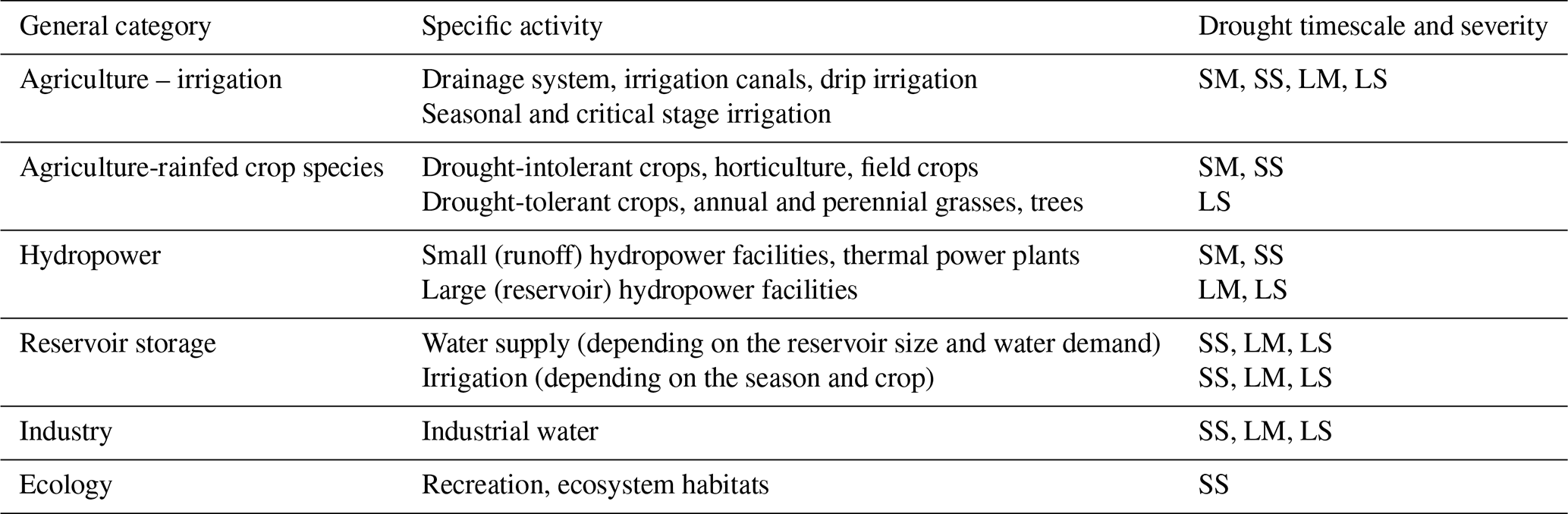
Table 3Timescale and severity classes of droughts for some specific activities. SM – short timescale and mild/moderate drought, SS – short timescale and severe/extreme drought, LM – long timescale and mild/moderate drought, LS – long timescale and severe/extreme drought, S – shorter than 6 months, L – 6 months or longer.
DI-based drought IDF curves do not incorporate site-specific precipitation and streamflow deficits of each month other than the drought indices. However, regional precipitation patterns, including intense and prolonged deficits, play a critical role in identifying frequency of drought and challenge to mitigate drought by established management plans (Kreibich et al., 2022). Short- and long-term deficits can be detected from the intensity of the drought indicators combined with duration and frequency. In particular, long-term droughts with high variations and frequently occurring intense deficits can be assessed as primary characteristics for determining site sensitivity, while regular and comparatively short deficits are general characteristics of the regional climate condition (Halwatura et al., 2015). The different patterns of summer precipitation and streamflow in the two case studies, Seyhan and Kocher, illustrated how seasonality becomes the primary factor of deficits. We found that short-timescale deficits are the most severe droughts with higher variability. The lower variability of longer timescales applied both to precipitation and streamflow. Implementation of the IDF curves on the drought events of 2008 in the Seyhan and 2018 in the Kocher demonstrated this reality and the impact of drought in these regions (Cavus et al., 2022; Tijdeman et al., 2022; Rakovec et al., 2022).
5.3 IDF curves for practice: timescale and severity
Deficit-IDF curves for the design under drought conditions have not been well established in literature and practice. There is an emerging need for guidelines worldwide to use in water resources design, planning, operation and management under low-flow or drought conditions (Vogel and Kroll, 2021). Similar to the precipitation IDF curves used in hydrological practice (Chow et al., 1988), deficit-IDF curves developed in this study can therefore be considered an improvement towards the design under drought conditions. In practical meaning, the timescale is the time lag between the initiation of water deficit and its impact on water resources, engineering activity, ecology, economy or society. An assessment about the choice of the timescales has been made by Vicente-Serrano et al. (2013) for vegetation, and Halwatura et al. (2015) for ecosystem establishment after mining. They divided the timescales into two; short and long timescales and provided a list of dominant timescales. However, the timescales can overlap and change from region to region or from season to season in the same region. For example, a short but severe drought might have the same impact as a long mild drought. For these reasons, we consider the applicability of IDF curves by timescale and severity of various activities.
Successful drought and water management requires knowledge of drought characteristics at varying timescales. Seasonal or even over-year water storage and release at longer timescales are important processes in some catchments and for some water uses, while in other catchments for other water needs, shorter-timescale variability matters as water needs to be provided regularly, e.g., for hydropower generation. Accordingly, different drought threats matter as the impacts are very different, and this will affect the usefulness of the IDF curves. This final section explores how IDF curves might be beneficial for management actions such as agriculture irrigation for different crops, industrial water uses and reservoir storage for different purposes or run-of-the-river hydropower, as well as for nature's water needs, such as aquatic ecology. Table 3 categorizes these water needs and the associated drought timescales and drought severity classes that threaten them.
Irrigation methods for agricultural activities require cost-effective drought management strategies for specific sites. The IDF curves of precipitation deficit of long timescales and moderate/severe droughts can provide a useful knowledge for larger area agriculture such as the design of drainage systems and irrigational canals (Table 3). For drip, seasonal and critical stage irrigation for which a lower amount of water is needed compared to larger drainage systems, short timescales provide important information about the deficit. Horticulture and field crops cannot resist against long-term deficits; i.e., any design for such activities should consider short timescales. For non-irrigated agriculture, precipitation deficit IDF can be used at short and long timescales, while for irrigated agriculture, streamflow deficit-IDF curves can be used at different timescales depending on the region and crop type. Long-timescale IDF curves can be considered for drought-tolerant species with deep roots. Regarding crop species, some specific crop types cannot grow if the drought exceeds a certain duration or intensity. For instance, precipitation deficit-IDF curves at short timescales are important for drought-intolerant crops while long timescales are important for drought-tolerant crops, annual and perennial grasses, and trees.
Diversion hydropower plants or thermal power plants as they often exist in Germany and also further downstream in the Kocher will be affected by droughts at short timescales, while storage hydropower plants as they often exist in the mountains or in semi-arid climates in the Mediterranean region will be interested in the threat from long droughts (Table 3). Short-timescale IDF curves based on streamflow deficit can provide useful information under mild/moderate drought conditions for river water uses for industry or for recreational use. Ecosystem habitats again might mostly require consideration at short timescales but during very specific seasons (spawning, migration time, oxygen depletion), but also longer periods when it comes to overall environmental degradation. The return periods of streamflow deficits provide the probability of deficits at these durations and intensities, and the risk of drought can be interpreted correctly. This is important for water managers who can conduct a cost–benefit analysis on whether the cost of taking some mitigation precautions such as agriculture, reservoir and hydropower is comparable with the cost of probable failure (Table 3). Selection of small hydropower management based on different timescales is also a key management action for deficit-IDF curves.
Another issue could be related to the temporal variability. A less variable system can be linked with a longer timescale, and a more variable system with a shorter timescale. Specifically, short-timescale streamflow deficit-IDF curves should be used for the run-of-the-river and pumped storage energy production plants because they have higher fluctuation in the river. The storage systems can be tolerant of long-timescale droughts if the storage is filled enough at the beginning of dry period. Therefore, long-timescale streamflow deficit-IDF curves work well for storage hydropower systems. For water supply systems, streamflow deficit-IDF curves at short timescales can be advised. The categorization outlined in this study (Table 3) clarifies the usefulness of the deficit-based IDF curves to address the site-specific climatic conditions. Drought IDF curves should be a primary factor of drought mitigation strategies and eventually help to guide water recourses management planning, where hydrological extremes have an impact on current operations.
We developed deficit-IDF curves to assess how associated deficits vary in a given catchment at different return periods although they have similar drought intensity in the drought index. We explained the advantage of using physical variables, precipitation and streamflow deficits, giving more practical and straightforward use to the deficit-IDF curves than the index-based drought IDF curves. This makes the new drought IDF curves generally applicable for different climatological regions and also for a comparison of their drought risks. Deficit IDF curves can be developed for any location or catchment to convert drought index values to deficit. Precipitation and streamflow deficits distinguish the degree of drought impact and its implication for various water uses. The use of IDF curves with the observed droughts showed their applicability in identifying return periods. A given value of both types of deficit has higher return periods at longer drought durations and lower return periods at shorter drought durations. Precipitation deficits of the observed major droughts are higher in amount but have lower return periods than their streamflow deficits. Here, we stress that deficits can be highly variable, which makes it necessary to comprehensively assess the usefulness of IDF curves before establishing drought mitigation strategies. Thanks to the deficit knowledge, drought intensity in a particular system can be interpreted correctly, especially that characterized by complex hydrological systems. Deficit IDF curves can be applied to quantify the frequency of drought events and characterized by intensity and duration at different timescales. Precipitation and streamflow deficits of droughts should be used to assess drought management strategies based on return periods.
The application here was limited to a few examples regarding indices, timescales and thresholds for station-based precipitation and streamflow deficits of droughts. The deficit-IDF curve approach of this study can also be adapted to drought indices other than the SPI or SSI and to threshold levels corresponding to different situations in terms of severity or even to impact-specific thresholds. How transferable the approach is to other indices and thresholds and also to other climates and hydrological regimes than the examples used here remains to be tested in order to assess the range of applicability. Further work might also explore the extension of station-based drought IDF curves to develop regional curves for possible use at ungauged basins.
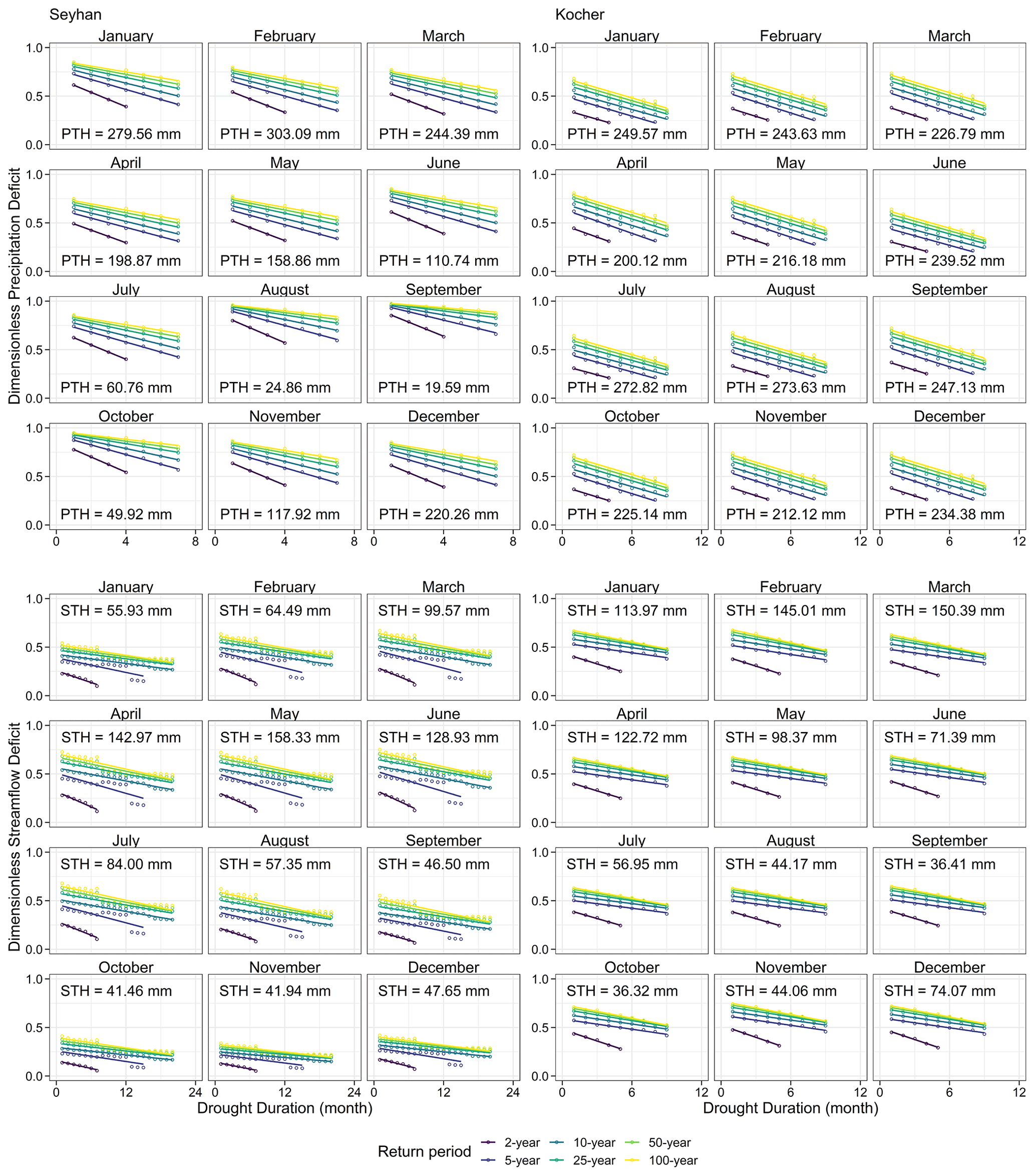
Figure A1Drought-IDF curves in terms of precipitation and streamflow deficit divided by the threshold value for the Seyhan and Kocher at a 3-month timescale.
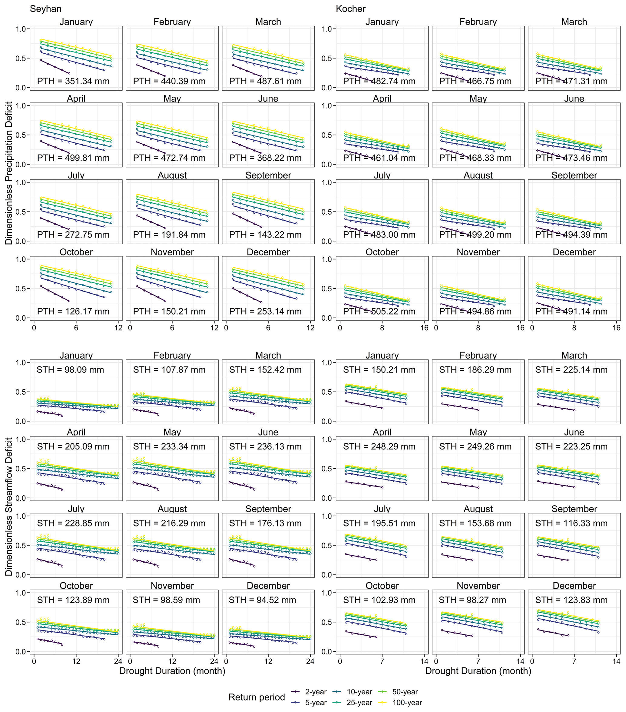
Figure A2Drought-IDF curves in terms of precipitation and streamflow deficit divided by the threshold value for the Seyhan and Kocher at a 6-month timescale.
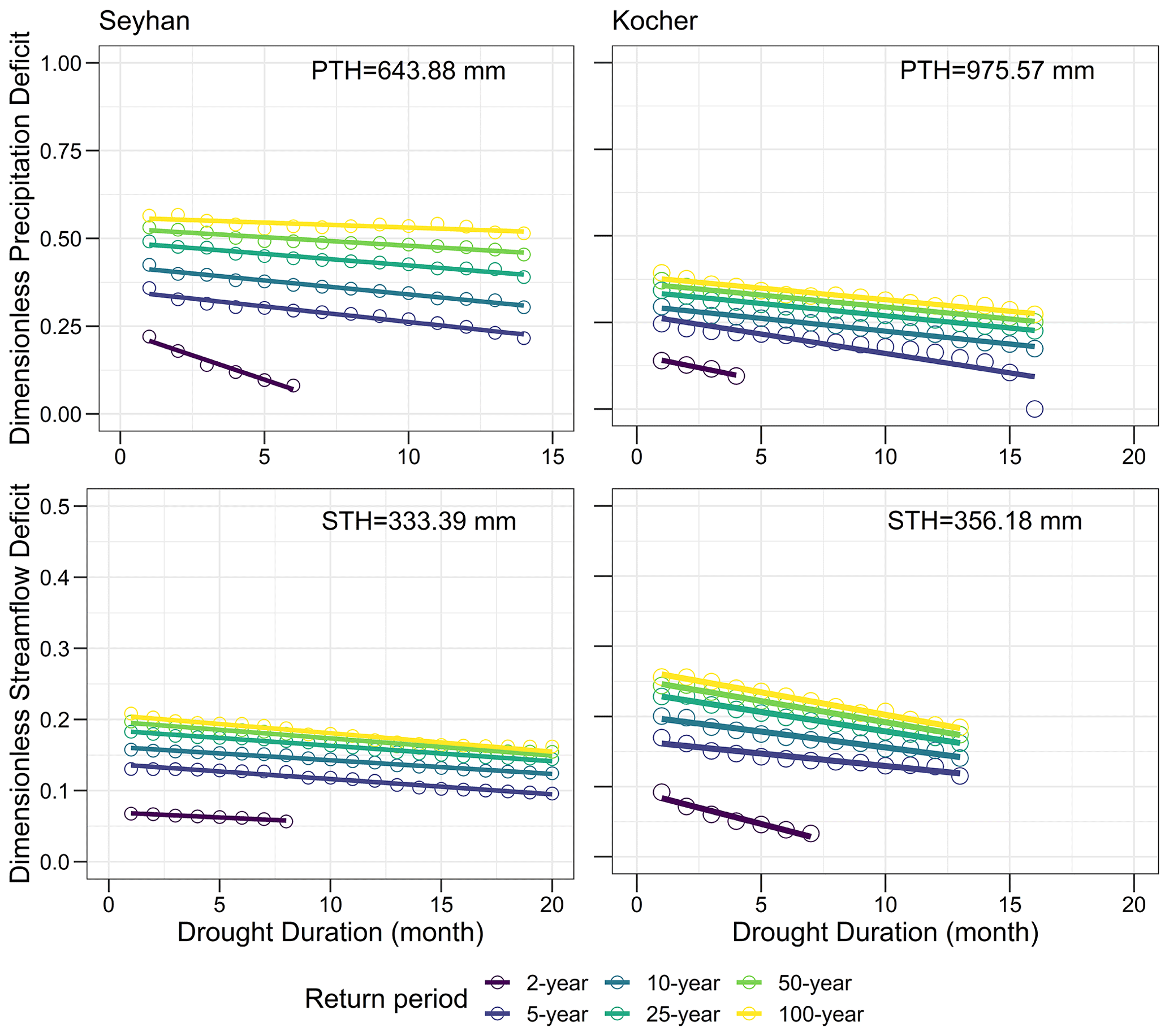
Figure A3Drought-IDF curves in terms of precipitation and streamflow deficit divided by the threshold value for the Seyhan and Kocher at a 12-month timescale.
Precipitation data provided by the Turkish State Meteorological Service (TSMS) can be purchased from https://mevbis.mgm.gov.tr/mevbis/ui/index.html (TSMS, 2023). Precipitation data provided by the German Weather Service (DWD) can be downloaded from https://opendata.dwd.de/climate_environment/CDC/observations_germany/ (DWD, 2023). Streamflow data provided by the general directorate of State Hydraulic Works (DSI) can be downloaded from https://www.dsi.gov.tr/Sayfa/Detay/744# (DSI, 2023). Streamflow data provided by the Environment Agency of Baden-Württemberg (LUBW) can be obtained on request (https://www.lubw.baden-wuerttemberg.de/startseite, last access: 14 April 2023).
YC: data curation, formal analysis, investigation, methodology, software, validation, visualization and writing (original draft, review and editing). KS: investigation, methodology, supervision and writing (review and editing). HA: investigation, methodology, supervision and writing (review and editing).
The contact author has declared that none of the authors has any competing interests.
Publisher's note: Copernicus Publications remains neutral with regard to jurisdictional claims in published maps and institutional affiliations.
This article is part of the special issue “Drought, society, and ecosystems (NHESS/BG/GC/HESS inter-journal SI)”. It is a result of the Panta Rhei Drought in the Anthropocene workshop 2022, Uppsala, Sweden, 29–30 August 2022.
We thank all data-providing organizations named in the “Data availability” section.
The first author was funded by the DAAD “Research
Grants – Bi-nationally Supervised Doctoral Degrees/Cotutelle”
program under grant no. 91772148.
This open-access publication was funded by the University of Freiburg.
This paper was edited by Khalid Hassaballah and reviewed by two anonymous referees.
Aksoy, H., Cetin, M., Eris, E., Burgan, H. I., Cavus, Y., Yildirim, I., and Sivapalan, M.: Critical drought intensity-duration-frequency curves based on total probability theorem-coupled frequency analysis, Hydrolog. Sci. J., 66, 1337–1358, https://doi.org/10.1080/02626667.2021.1934473, 2021.
Brunner, M. I., Liechti, K., and Zappa, M.: Extremeness of recent drought events in Switzerland: dependence on variable and return period choice, Nat. Hazards Earth Syst. Sci., 19, 2311–2323, https://doi.org/10.5194/nhess-19-2311-2019, 2019.
Cavus, Y. and Aksoy, H.: Spatial drought characterization for Seyhan River basin in the Mediterranean region of Turkey, Water, 11, 1331, https://doi.org/10.3390/w11071331, 2019.
Cavus, Y. and Aksoy, H.: Critical drought severity/intensity-duration-frequency curves based on precipitation deficit, J. Hydrol., 584, 124312, https://doi.org/10.1016/j.jhydrol.2019.124312, 2020.
Cavus, Y., Stahl, K., and Aksoy, H.: Revisiting Major dry periods by rolling time series analysis for human-water relevance in drought, Water Resour. Manag., 36, 2725–2739, https://doi.org/10.1007/s11269-022-03171-8, 2022.
Chow, V. T., Maidment, D. R., and Mays, L. W.: Applied Hydrology, McGraw-Hill, New York, USA, ISBN: 0-07-010810-2, 1988.
Dalezios, N. R., Loukas, A., Vasiliades L., and Liakopoulos, E.: Severity-duration-frequency analysis of droughts and wet periods in Greece, Hydrolog. Sci. J., 45:5, 751–769, https://doi.org/10.1080/02626660009492375, 2000.
GDWM: Seyhan basin drought management plan, Ministry of Forestry and Water Affairs, General Directorate of Water Management, Flood and Drought Management Department, Final Report, Executive Summary, Ankara, 2019.
German Weather Service (DWD): Precipitation Data, DWD [data set], https://opendata.dwd.de/climate_environment/CDC/observations_germany/, last access: 14 April 2023.
Gupta, V., Jain, M. K., and Singh, V. P.: Multivariate modelling of projected drought frequency and hazard over India, ASCE J. Hydrol. Eng., 25, 04020003, https://doi.org/10.1061/(ASCE)HE.1943-5584.0001893, 2020.
Haan, C. T.: Statistical Methods in Hydrology, Iowa State University Press, Ames, lowa, USA, ISBN 0-8138-1510-X, 9780813815107, 1977.
Halwatura, D., Lechner, A. M., and Arnold, S.: Drought severity–duration–frequency curves: a foundation for risk assessment and planning tool for ecosystem establishment in post-mining landscapes, Hydrol. Earth Syst. Sci., 19, 1069–1091, https://doi.org/10.5194/hess-19-1069-2015, 2015.
Kreibich, H., Van Loon, A. F., Schröter, K., Ward, P. J., Mazzoleni, M., Sairam, N., Abeshu, G. W., Agafonova, S., AghaKouchak, A., Aksoy, H., Alvarez-Garreton, C., Aznar, B., Balkhi, L., Barendrecht, M. H., Biancamaria, S., Bos-Burgering, L., Bradley, C., Budiyono, Y., Buytaert, W., Capewell, L., Carlson, H., Cavus, Y., Couasnon, A., Coxon, G., Daliakopoulos, I., de Ruiter, M. C., Delus, C., Erfurt, M., Esposito, G., François, D., Frappart, F., Freer, J., Frolova, N., Gain, A. K., Grillakis, M., Grima, J. O., Guzmán, D. A., Huning, L. S., Ionita, M., Kharlamov, M., Khoi, D. N., Kieboom, N., Kireeva, M., Koutroulis, A., Lavado-Casimiro, W., Li, H., Llasat, M. C., Macdonald, D., Mård, J., Mathew-Richards, H., McKenzie, A., Mejia, A., Mendiondo, E. M., Mens, M., Mobini, S., Mohor, G. S., Nagavciuc, V., Ngo-Duc, T., Nguyen, H. T. T., Nhi, P. T. T., Petrucci, O., Quan, N. H., Quintana-Seguí, P., Razavi, S., Ridolfi, E., Riegel, J., Sadik, M. S., Savelli, E., Sazonov, A., Sharma, S., Sörensen, J., Souza, F. A. A., Stahl, K., Steinhausen, M., Stoelzle, M., Szalińska, W., Tang, Q., Tian, F., Tokarczyk, T., Tovar, C., Tran, T. V. T., Van Huijgevoort, M. H. J., van Vliet, M. T. H., Vorogushyn, S., Wagener, T., Wang, Y., Wendt, D. E., Wickham, E., Yang, L., Zambrano-Bigiarini, M., Blöschl, G., and Di Baldassarre, G.: The challenge of unprecedented floods and droughts in risk management, Nature, 608, 80–86, https://doi.org/10.1038/s41586-022-04917-5, 2022.
McKee, T. B., Doesken, N. J., and Kleist, J.: The relationship of drought frequency and duration to time scales, Eighth Conference on Applied Climatology, American Meteorological Society, 17–23 January 1993, Anaheim CA, 179–184, 1993.
Pandya, P. and Gontia, N. K.: Development of drought severity–duration–frequency curves for identifying drought proneness in semi-arid regions, J. Water Clim Change, 14, 824–842 https://doi.org/10.2166/wcc.2023.438, 2023.
Rakovec, O., Samaniego, L., Hari, V., Markonis, Y., Moravec, V., Thober, S., Hanel, M., and Kumar, R.: The 2018–2020 multi-year drought sets a new benchmark in Europe, Earths Future, 10, e2021EF002394, https://doi.org/10.1029/2021EF002394, 2022.
Reddy, M. J. and Ganguli, P.: Application of copulas for derivation of drought severity–duration–frequency curves, Hydrol. Process., 26, 1672–1685, https://doi.org/10.1002/hyp.8287, 2012.
Sahana, V., Sreekumar P., Mondal, A., and Rajsekhar, D.: On the rarity of the 2015 drought in India: A country-wide drought atlas using the multivariate standardized drought index and copula-based severity-duration-frequency curves, Journal of Hydrology: Regional Studies, 31, 100727, https://doi.org/10.1016/j.ejrh.2020.100727, 2020.
Shiau, J. T. and Modarres, R.: Copula-based drought severity-duration-frequency analysis in Iran, Meteorol. Appl., 16, 481–489, https://doi.org/10.1002/met.145, 2009.
Sit, V. and Poulin-Costello, M.: Catalog of Curves for Curve Fitting, Biometrics Information Handbook Series No. 4, Province of British Columbia Ministry of Forests, Victoria, BC, Canada, ISBN 0-7726-2049-0, 1994.
State Hydraulic Works (DSI): Streamflow Data, DSI [data set], https://www.dsi.gov.tr/Sayfa/Detay/744#, last access: 14 April 2023.
Sung, J. H. and Chung, E.-S.: Development of streamflow drought severity–duration–frequency curves using the threshold level method, Hydrol. Earth Syst. Sci., 18, 3341–3351, https://doi.org/10.5194/hess-18-3341-2014, 2014.
Tijdeman, E., Stahl, K., and Tallaksen,L. M.: Drought characteristics derived based on the Standardized Streamflow Index: A large sample comparison for parametric and nonparametric methods, Water Resour. Res., 56, e2019WR026315, https://doi.org/10.1029/2019WR026315, 2020.
Tijdeman, E., Blauhut, V., Stoelzle, M., Menzel, L., and Stahl, K.: Different drought types and the spatial variability in their hazard, impact, and propagation characteristics, Nat. Hazards Earth Syst. Sci., 22, 2099–2116, https://doi.org/10.5194/nhess-22-2099-2022, 2022.
Todisco, F., Mannocchi, F., and Vergni, L.: Severity–duration–frequency curves in the mitigation of drought impact: an agricultural case study, Nat. Hazards 65, 1863–1881, https://doi.org/10.1007/s11069-012-0446-4, 2013.
Turkish State Meteorological Service (TSMS): Precipitation Data, TSMS [data set] https://mevbis.mgm.gov.tr/mevbis/ui/index.html, last access: 14 April 2023.
url1: The European Drought Observatory, Emergency Management Service, Copernicus, https://edo.jrc.ec.europa.eu/, last access: 14 April 2023.
url2: Drought Analysis, Turkish State Meteorological Service, https://mgm.gov.tr/veridegerlendirme/kuraklik-analizi.aspx, last access: 14 April 2023.
url3: Drought Index, Deutscher Wetterdienst, https://www.dwd.de/EN/ourservices/rcccm/int/rcccm_int_spi.html, last access: 14 April 2023.
url4: Niedrigwasser-Lagebericht Bayern, Bayerisches Landesamt für Umwelt, https://www.nid.bayern.de, last access: 14 April 2023).
Van Loon, A. F.: Hydrological drought explained, WIREs Water, 2: 359-392, https://doi.org/10.1002/wat2.1085, 2015.
Vicente-Serrano, S. M., Lopez-Moreno, J. I., Beguería, S., Lorenzo-Lacruz, J., Azorin-Molina, C., and Moran-Tejeda, E.: Accurate computation of a streamflow drought index, J. Hydrol. Eng., 17, 318–332, https://doi.org/10.1061/(ASCE)HE.1943-5584.0000433, 2012.
Vicente-Serrano, S. M., Gouveia, C., Camarero, J. J., Beguería, S., Trigo, R., López-Moreno, J. I., Azorín-Molina, C., Pasho, E., Lorenzo-Lacruz, J., Revuelto, J., Morán-Tejeda, E., and Sanchez-Lorenzo, A.: Response of vegetation to drought time-scales across global land biomes, P. Natl. Acad. Sci. USA, 110, 52–57, https://doi.org/10.1073/pnas.1207068110, 2013.
Vogel, R. M. and Kroll, C. N.: On the need for streamflow drought frequency guidelines in the US, Water Policy, 23, 216, https://doi.org/10.2166/wp.2021.244, 2021.
Wu, H., Hayes, M. J., Wilhite, D. A., and Svoboda, M. D.: The effect of the length of record on the standardized precipitation index calculation, Int. J. Climatol., 25, 505–520, https://doi.org/10.1002/joc.1142, 2005.
Zeitler, F., Dotterweich, M., and Rothstein, B.: Nutzungskonflikte bei zukünftigen Niedrigwasserständen, Analyse + Ableitung von Handlungsempfehlungen an den Beispielen Murg und Kocher, Klimawandel und modellhafte Anpassung in Baden-Württemberg, LUBW Landesanstalt für Umwelt Baden-Württemberg, 2017.