the Creative Commons Attribution 4.0 License.
the Creative Commons Attribution 4.0 License.
 | 08 Sep 2023
Calibration of groundwater seepage against the spatial distribution of the stream network to assess catchment-scale hydraulic properties
Ronan Abhervé
Clément Roques
Alexandre Gauvain
Laurent Longuevergne
Stéphane Louaisil
Luc Aquilina
Jean-Raynald de Dreuzy
The assessment of effective hydraulic properties at the catchment scale, i.e., hydraulic conductivity (K) and transmissivity (T), is particularly challenging due to the sparse availability of hydrological monitoring systems through stream gauges and boreholes. To overcome this challenge, we propose a calibration methodology which only considers information from a digital elevation model (DEM) and the spatial distribution of the stream network. The methodology is built on the assumption that the groundwater system is the main driver controlling the stream density and extension, where the perennial stream network reflects the intersection of the groundwater table with the topography. Indeed, the groundwater seepage at the surface is primarily controlled by the topography, the aquifer thickness and the dimensionless parameter , where R is the average recharge rate. Here, we use a process-based and parsimonious 3D groundwater flow model to calibrate by minimizing the relative distances between the observed and the simulated stream network generated from groundwater seepage zones. By deploying the methodology in 24 selected headwater catchments located in northwestern France, we demonstrate that the method successfully predicts the stream network extent for 80 % of the cases. Results show a high sensitivity of to the extension of the low-order streams and limited impacts of the DEM resolution as long the DEM remains consistent with the stream network observations. By assuming an average recharge rate, we found that effective K values vary between and m s−1, in agreement with local estimates derived from hydraulic tests and independent calibrated groundwater model. With the emergence of global remote-sensing databases compiling information on high-resolution DEM and stream networks, this approach provides new opportunities to assess hydraulic properties of unconfined aquifers in ungauged basins.
- Article
(5679 KB) - Full-text XML
-
Supplement
(5157 KB) - BibTeX
- EndNote


Evaluating the availability of water resources and its evolution under global changes requires a quantitative assessment of water fluxes at the catchment scale (Fan et al., 2019). Such an evaluation involves the development of advanced hydrological models resolving relevant hillslope- to catchment-scale processes (Refsgaard et al., 2010; Holman et al., 2012; Wada et al., 2010) in a wide variety of high-stake areas (Elshall et al., 2020; Vergnes et al., 2020). Within the local hydrological cycle, aquifers ensure the storage of water during and after recharge periods, increasing the availability of the resources (Fan, 2015; Fan et al., 2015), and transfer this water to surface systems during rain-free periods (Winter, 1999; Sophocleous, 2002; Alley et al., 2002; Anderson et al., 2015). Quantifying groundwater fluxes remains a challenge, as the hydraulic properties of aquifers, i.e., hydraulic conductivity (K) and transmissivity (T), have classically been constrained through sparse borehole-scale characterization (Anderson et al., 2015; Carrera et al., 2005). They are classically estimated using hydraulic tests at centimeter scales for laboratory experiments up to decameter scales for well tests (Renard, 2005; Freeze and Cherry, 1979; Domenico and Schwartz, 1990). Other methods have been proposed at larger scales based on the analysis of streamflow dynamics (Troch et al., 2013; Mendoza et al., 2003; Vannier et al., 2014; Brutsaert and Nieber, 1977), earth tides (Hsieh et al., 1987; Rotzoll and El-Kadi, 2008) and borehole head dynamics (Zlotnik and Zurbuchen, 2003; Jiménez-Martínez et al., 2013) as well as from the calibration of large-scale hydrological models (Eckhardt and Ulbrich, 2003; Etter et al., 2020; Chow et al., 2016). Multi-objective calibration has been proposed to reduce uncertainties, considering complementary data like temperature (Bravo et al., 2002), groundwater ages derived from environmental tracers (Kolbe et al., 2016) or continuous geochemical monitoring (Schilling et al., 2019). In addition, recent advances in machine learning technics show promising results to evaluate hydraulic properties at the regional scale (Cromwell et al., 2021; Marçais and de Dreuzy, 2017; Reichstein et al., 2019).
To tackle the numerous challenges related to the upscaling of hydraulic properties from the local to the regional or global scales, several databases provide exhaustive compilations of measurements performed all around the world (Comunian and Renard, 2009; Achtziger-Zupančič et al., 2017; Ranjram et al., 2015; Kuang and Jiao, 2014). By compiling values obtained from calibrated groundwater models, Gleeson et al. (2014) proposed a global-scale hydraulic conductivity map (GLobal HYdrogeology MaPS, GLHYMPS), with an update by Huscroft et al. (2018), where values have been interpolated based on a high-resolution Global LIthological Map (GliM; Hartmann and Moosdorf, 2012). Besides inconsistencies and methodological biases supported in Gleeson et al. (2014), the compiled permeabilities above the regional scale (>5 km) are not suitable at the catchment scale. Therefore, estimating subsurface hydraulic properties that correctly represent observed catchment-scale processes remains a major challenge for the hydrological community (Blöschl et al., 2019). New opportunities have been identified through the increasing availabilities of surface observations (Beven et al., 2020; Gleeson et al., 2021), specifically with an application for ungauged basins.
Information on the spatial distribution of groundwater seepage appears to be a critical observation to use for the calibration of subsurface hydraulic properties in hydrologic models (Grayson and Blöschl, 2000). This approach can be applied on the assumption that the density and extent of the stream network is primarily controlled by groundwater flow. This assumption is valid in temperate and wet climates for unconfined aquifers, where surface and subsurface hydrological systems are well connected (Cuthbert et al., 2019; Fan et al., 2013) with important discharge of the aquifer directly into the streams (Haitjema and Mitchell-Bruker, 2005). Indeed, a groundwater seepage network dominantly controls the structure of a continuous-stream network, its spatial extent and its ramification (De Vries, 1994; Devauchelle et al., 2012; Strahler, 1964; Leibowitz et al., 2018; Pederson, 2001). Under steady-state conditions, the distribution of groundwater seepage is then controlled by the characteristic hillslope geometry, the recharge rate (R) and the aquifer transmissivity (T), i.e., the product of the hydraulic conductivity (K) and the saturated aquifer thickness (dsat) (Litwin et al., 2022; Luijendijk, 2021; Bresciani et al., 2014; Haitjema and Mitchell-Bruker, 2005; Gleeson and Manning, 2008). At a given recharge rate, low transmissive aquifers display high groundwater table elevations and, consequently, dense stream networks in the upper part of the catchments. Conversely, highly transmissive aquifers will display lower groundwater tables, higher discharge rates in fewer seepage areas and, consequently, sparser stream networks confined in the lower-elevation valleys (Day, 1980; Lovill et al., 2018; Dunne, 1975; Luo et al., 2016; Dietrich and Dunne, 1993; Godsey and Kirchner, 2014; Prancevic and Kirchner, 2019).
Previous studies have focused on the comparison of an observed hydrographic network with a simulated hydrographic network computed from different methods. The organization of stream networks has been predicted directly from a digital elevation model (DEM) based on a predefined accumulation threshold value determining whether an upstream surface is capable of producing significant flow (Mardhel et al., 2021; Le Moine, 2008; Schneider et al., 2017; Luo and Stepinski, 2008; Lehner et al., 2013). Lumped parameter models, such as TOPMODEL (Beven and Kirkby, 1979), have also been extensively used to predict the spatial patterns of seepage areas (Merot et al., 2003) allowing us to constrain the subsurface hydraulic properties (Blazkova et al., 2002; Güntner et al., 2004; Franks et al., 1998). Luo et al. (2010) proposed a method leading to a spatial distribution of hydraulic conductivities by constraining a 1D groundwater model based on the Dupuit–Forcheimer (DF) assumption on drainage dissection patterns. However, these approaches are limited to considering a subsurface flow path equal and parallel to the downslope topography (Luo and Stepinski, 2008). Relying on explicit simulations of the spatial stream network with a process-based hillslope model following the DF assumption (Weiler and McDonnell, 2004), Stoll and Weiler (2010) proposed to overcome this limitation by routing the downslope subsurface flow from the groundwater table with a grid cell by grid cell approach (Wigmosta and Lettenmaier, 1999). The assessed subsurface hydraulic properties are intended to guide the calibration of hydrological models in ungauged basins, using only a DEM and a hydrographic network map. These approaches are especially relevant as rapid advances in remote sensing are improving the description of global river networks (Schneider et al., 2017; Lehner and Grill, 2013), wetlands (Tootchi et al., 2019; Rapinel et al., 2023) and soil moisture (Vergopolan et al., 2021). Lidar and high-resolution satellite imagery offer new opportunities to determine the surface characteristics of landscapes (Levizzani and Cattani, 2019; Blöschl et al., 2019) and, by extension, the hydrological parameters of local to continental ungauged catchments (Barclay et al., 2020; Dembélé et al., 2020).
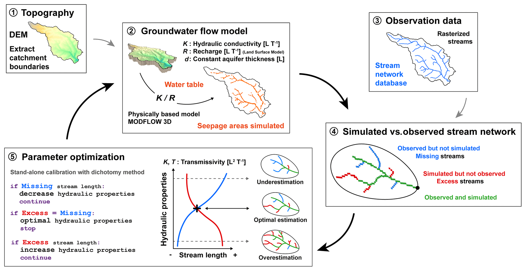
Figure 1Model workflow for the calibration of subsurface hydraulic properties from the observed stream network.
In this work, we propose a new methodology to quantify effective hydraulic properties of unconfined aquifers from topographical and stream network observations now available at high resolution. From a parsimonious 3D groundwater flow model, we aim at estimating the catchment-scale K, based on surface information only, which is the spatial distribution of the stream network. We propose a novel performance criterion to assess the similarity between the simulated seepage areas and the observed stream network, coupled with a stand-alone calibration procedure. We present the full methodology and its sensitivity to different hydrographic network observation products in 24 catchments covering various geological contexts in northwestern France. We finally discuss opportunities and perspectives to systematically characterize aquifers in ungauged catchments from surface observations.
An overview of the method workflow is illustrated in Fig. 1. Each block refers to a specific subsection detailed below (from Sect. 2.1 to 2.5).
-
A digital elevation method (DEM) is used as the top boundary of the groundwater flow model (Sect. 2.1).
-
Three-dimensional groundwater flow is solved in the model domain, and simulated seepage areas are extracted (Sect. 2.2).
-
A selected stream network independent of the DEM is taken as the observed reference (Sect. 2.3).
-
The dimensionless ratio [–] is calibrated to reach the best match between the simulated seepage areas and the extent of the observed stream network (Sect. 2.4).
-
From the optimized , the optimal hydraulic conductivity Koptim [L T−1] is deduced by considering the recharge R. The optimal transmissivity Toptim [L2 T−1] is obtained considering the average thickness of the saturated aquifer dsat [L] computed by the model (Sect. 2.5).
2.1 Definition of the model domain based on the analysis of the topography
We first select the digital elevation model (DEM) that will be defined as the upper boundary of the groundwater model. In this study, we use the 75 m grid resolution DEM available at the scale of France. It is generated from photogrammetric restitution and provided by BD ALTI (IGN, 2021). We also explore the impact of different DEM resolutions on the final estimations of . We consider two higher-resolution DEMs of 5 and 25 m also provided by BD ALTI. For coarser resolutions, the 25 m DEM was downsampled with the nearest-neighbor option to larger cell sizes, i.e., 100, 200 and 300 m.
Geospatial processing is performed using the software WhiteboxTools available in Python (Lindsay, 2016), labeled WBT with the respective functions quoted in brackets in the following. First, the raw DEM is corrected by filling all depressions and by removing flat areas (WBT.FillDepressions) to ensure continuous flow between grid cells. The vector point shapefile of the outlet is moved to the location coincident with the highest flow accumulation value (WBT.D8FlowAccumulation) within a specified maximum distance taken as twice the DEM resolution (e.g., 150 m for a 75 m resolution DEM) (WBT.SnapPourPoints). A flow direction raster (WBT.D8Pointer) is used to extract the drainage basin (WBT.Watershed).
2.2 Groundwater flow model parameterization
The MODFLOW software suite (Harbaugh, 2005) is used to solve the groundwater flow equation under steady-state conditions for an unconfined aquifer using a three-dimensional finite-difference approach (Harbaugh, 2005; Niswonger et al., 2011). The hydraulic head, h [L], is calculated as a function of the hydraulic conductivity, K [L T−1], and the recharge rate, R [L T−1], applied on top of the water column. At the surface of the model domain, the drain package (DRN) of MODFLOW accounts for the intersection of the groundwater table with the surface and for the induced seepage. Overland flows and surface water re-infiltration are not integrated as they remain marginal in the conditions of temperate climate and low topographical gradients of the studied sites.
We use the FloPy Python package (Bakker et al., 2016) to set and handle simulations. To reduce uncertainties linked to potential flow across topographic boundaries, a buffer zone is added to the topographical catchment boundaries, increasing the modeled domain area by 10 %. The 3D model domain is discretized laterally using the regular mesh of the DEM and vertically into six layers of equal thickness. Convergence tests are performed to ensure the stability of the result independently of numerical discretization. In agreement with field observations undertaken in the region, a homogeneous thickness of the aquifer, d [L], is set to a constant value of 30 m. This thickness represents the typical depth of the interface between the shallow weathered and/or fractured zone with the underlying fresh bedrock (Dewandel et al., 2006; Roques et al., 2016; Mougin et al., 2008; Kolbe et al., 2016). The model assumes a uniform and isotropic hydraulic conductivity.
The recharge is estimated by the land EXternalized SURFace model (SURFEX version 8.1; Le Moigne et al., 2020). For more detailed information, the reader is referred to https://www.umr-cnrm.fr/surfex/ (last access: 1 September 2023). Supplied by meteorological variables, SURFEX computes the energy and water fluxes at the interfaces between soil, vegetation and the atmosphere (Noilhan and Mahfouf, 1996). The groundwater recharge of SURFEX is computed as the proportion of the water mobilized down to the aquifer after infiltrating through the soil column (Vergnes et al., 2020). SURFEX was supplied by the SAFRAN meteorological reanalysis (Vidal et al., 2010; Quintana-Seguí et al., 2008), available over the French metropolitan area at a 64 km2 (8×8 km) resolution. Here, we took the steady-state recharge as the long-term average recharge rates computed over the period 1960–2019 and applied them uniformly over the surface of the 3D domain.
2.3 Spatial distribution of the observed stream network
The observed stream network is extracted from the French hydrographic network database BD TOPAGE as a vector format at the scale of 1:10 000 (IGN and OFB, 2019). The main vector file labeled “Cours d'eau” (rivers) of BD TOPAGE represents the majority of perennial sections of the stream network, i.e., filled and/or continuous-flow segments throughout the year. Note that the information classifying perennial or intermittent streams collected in the database is still under development to increase accuracy (Schneider et al., 2017). It has been rasterized at a grid resolution similar to the groundwater flow model in order to facilitate the comparison of the results (WBT.VectorLinesToRaster). Due to the uncertainty in the positioning of the stream network vector with respect to the DEM, an error of the order of 1 pixel is considered (plus or minus 75 m in this case). The influence of this error is analyzed in the results presented in Sect. 3.1 (Fig. 4). We also quantify the impacts of other DEM product resolutions by considering five other hydrographic network products from three different sources: the global-scale database HydroRIVERS (labeled case A), the French database BD TOPAGE (cases B, C and D) and local-scale inventories (cases E and F) performed within the framework of SAGE (Schéma d'Aménagement et de Gestion des Eaux). The HydroRivers product is derived from the processing of the DEM at lower resolution (approximately 500 m at the Equator), while the local inventories are completed by more detailed field observations. More information on these products can be found in Appendix A.
2.4 Calibration criteria between observed and simulated spatial patterns
For each pixel where seepage is simulated by the groundwater flow model, we trace the nearest downslope flow path to the observed stream and compute its distance Dso [L] (WBT.TraceDownslopeFlowpaths) (Fig. 2a). This function of WhiteboxTools uses the topographic structure to compute the path from cells on the surface to the catchment outlet. This procedure converts the initial discontinuous spatial pattern of seepage zones simulated by the groundwater flow model into a continuous-stream network (Fig. 2b).
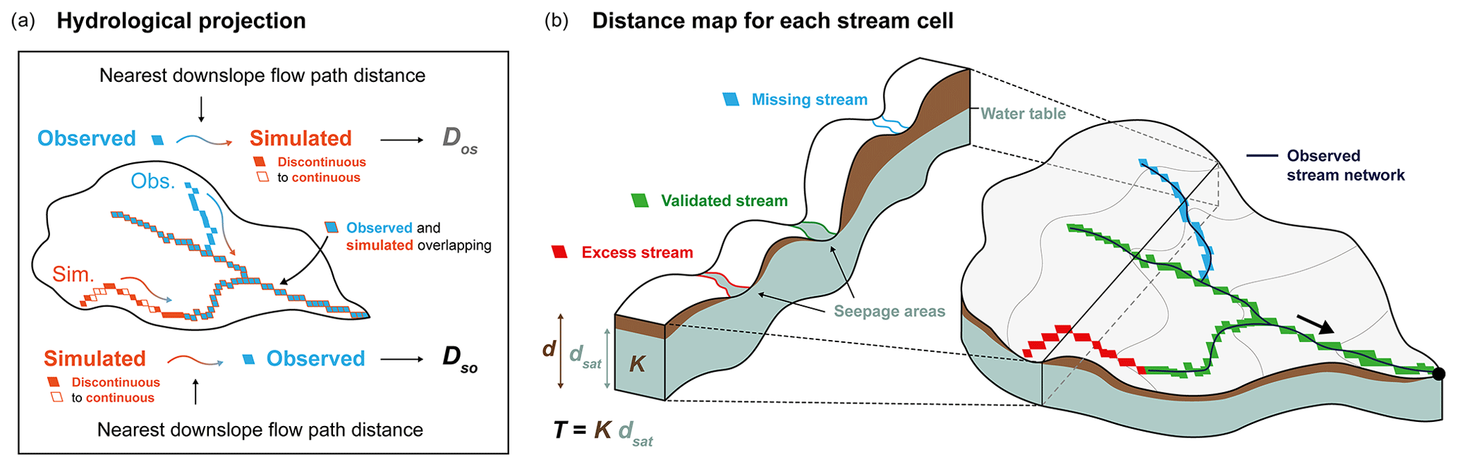
Figure 2(a) Definition of the main metrics used for calibration, with , the average distances computed from simulated stream pixels (in orange) to the nearest (downslope flow path) observed stream pixels (in blue) and the average distances obtained conversely. (b) Three-dimensional conceptual diagram of the groundwater flow model and of a cross section through the catchment. Continuous streams are generated from pixels where the simulated groundwater table intercepts the topography. By comparison with the observed stream network, some of the simulated streams are correctly estimated (valid, in green), overestimated (excess, in red) or underestimated (missing, in blue).
The distances of the simulated stream network to the observed Dso are calculated and averaged into the criterion labeled (WBT.DownslopeDistanceToStream). High values are characteristic of stream networks extending far away from the observed steams. We also compute the mean distance of the observed to the simulated stream networks following a similar procedure. The distance Dos [L] from each observed stream network pixel to the simulated stream is computed along the steepest downslope path. In the following, we consider its average obtained over all pixels of the observed streams. High values are characteristic of an underdeveloped stream network. The minimum absolute difference between and (Eq. 1), labeled J, is used as the calibration criterion expressing the closest match of the observed and simulated streams or, in other words, the most relevant combination of missing and excess streams (Fig. 2):
and intersect when the calibration criterion J is met. This criterion based on both and achieves the best equilibrium between over- and underestimations.
At this point, we define the distance Doptim [L] as the average of and (Eq. 2):
The smaller the value of Doptim, the better the match of the simulated seepage pattern and the observed stream network. Doptim will thus be used as an indicator of the calibration performance. In order to compare cases with different DEM resolution DEMres [L], Doptim is normalized by the DEM resolution:
roptim [–] should remain small to ensure the consistency of the observed and simulated stream networks. It will practically be limited to 2 considering that the mismatch cannot exceed the resolution of 2 pixels:
2.5 Estimating the optimal hydraulic conductivities
The model parameter ratio is calibrated by minimizing the objective function defined by Eq. (1), for a given aquifer thickness (d). Optimization is performed by a dichotomy approach (Burden and Faires, 1985). The convergence criterion is reached when varies by less than 1 %. In order to ensure that K estimates are representative of catchment-scale processes driving the spatial distribution of the stream network, independently of the aquifer thickness set in the model, we computed the equivalent normalized transmissivity, , by multiplying by the average saturated aquifer thickness (dsat) computed by the model at the catchment scale (Fig. 2b). In our modeling approach, K and d are input parameters of the model, while T is an output including the computed dsat. Finally, optimal transmissivity Toptim and hydraulic conductivity Koptim are evaluated assuming the applied average groundwater recharge rate, R, and with known aquifer thickness.
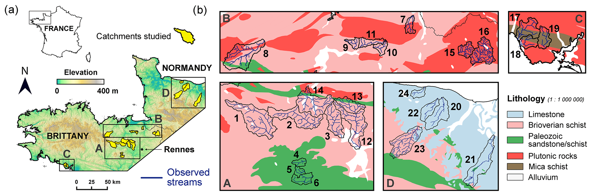
Figure 3(a) Location of the pilot catchments (Armorican Massif in Brittany and Normandy, northwestern part of France). (b) Zoom on sites along with a simplified map of the main lithological units (1:1 000 000 scale) in sub-panels A, B, C and D.
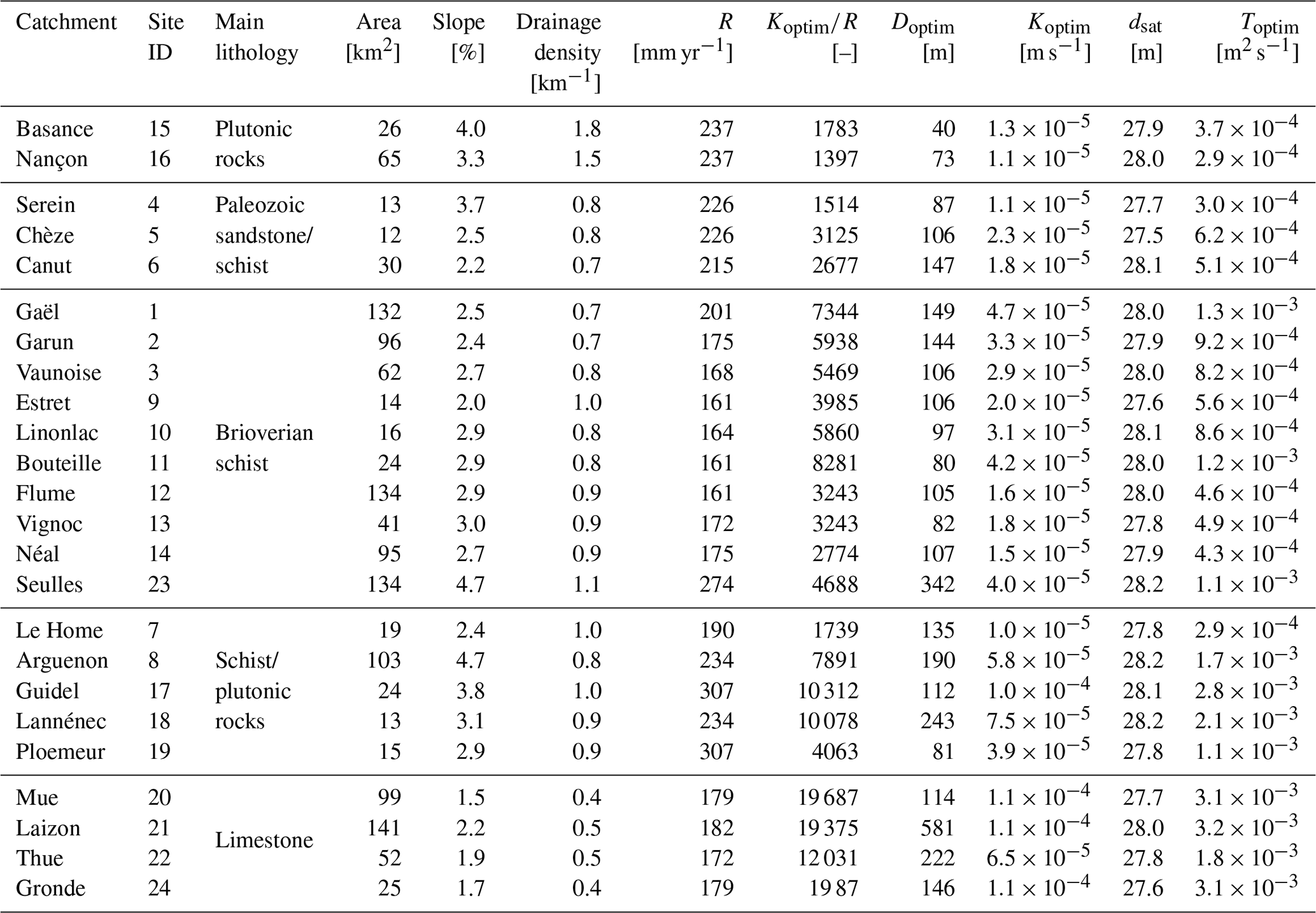
Table 1Main landscape characteristics, model input parameters and modeling results, including hydraulic conductivities and transmissivities for the 24 catchments studied.
2.6 Testing the methodology on selected pilot catchments
The approach is deployed in 24 selected catchments located in Brittany and Normandy (France) (Fig. 3), where an oceanic and temperate climate prevails. The average catchment area ranges from 12 to 141 km2 with an average of 58 km2 (Table 1), which corresponds to an average of 61 800 elements for the domain model discretization. These catchments were selected because of the diversity of their geological and geomorphological settings. Most of them are also subject to extensive research activities for their importance in providing freshwater to the nearby cities (sites 1, 2, 3, 4, 5, 6, 15, 16, 18, 19) or flooding dynamics (sites 20, 21, 22, 23, 24). Some of these sites are also studied in collaboration with local stakeholders in issues related to water quality and river restoration (sites 8, 9, 10, 11, 12, 13, 14, 17, 18 19) or within observatories and research infrastructures (site 7: long-term socio-ecological research (LTSER) “Zone Atelier Armorique (ZAAr)”; sites 17, 18, 19: French network of Critical Zone Observatories (OZCAR) “Ploemeur-Guidel CZO”). None of these catchments present any reservoir or stream obstacle that would significantly alter the stream network. The study sites cover five major lithologies including Brioverian schist (sedimentary rock), Paleozoic sandstone and schist (sedimentary rock), plutonic rocks (mainly granite), mica schist (metamorphic sedimentary rock), and limestone (sedimentary rock). Sites have a homogeneous lithology (1:1 000 000 scale) throughout the catchment except for five sites (sites 7, 8, 17, 18, 19) that present two lithologies.
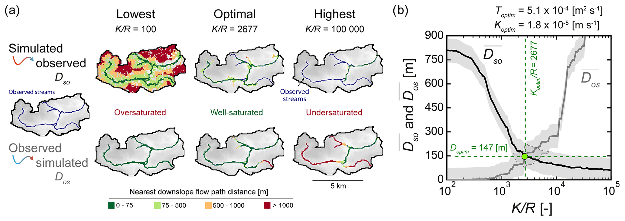
Figure 4(a) Two-dimensional map views of distances computed along the steepest slope from simulated stream pixels to the nearest observed ones (Dso) and from the observed stream pixels to the nearest simulated ones (Dos) for the Canut catchment. Results are presented for the lowest, optimal and highest values explored. (b) Average distances and as functions of . The shaded areas in gray around the curves correspond to the 75 m uncertainty range equal to the resolution the DEM. The optimal simulation is obtained for at the intersection between the two curves. At this point and are both equal to Doptim, and, in this case, roptim is close to 2. The estimated optimal hydraulic conductivity Koptim is derived by using the recharge rate provided by SURFEX, and Toptim is obtained considering the mean saturated aquifer thickness (dsat). To further illustrate the methodology, an animated figure representing 2D map views of the simulated seepage areas as a function of is available in the Supplement with the associated objective minimization function results in Appendix B.
3.1 Detailed analysis of model results at a single site
Before presenting the results obtained for the ensemble of pilot sites, we first illustrate the results of the methodology at one specific site, the Canut catchment (Fig. 3, site 6). We provide details on the different steps of the numerical method and assess their performance. The main results of the calibration method are presented in Fig. 4. The dimensionless ratio strongly controls the spatial distribution of the hydraulic head, i.e., the saturated aquifer thickness dsat, the shape of the groundwater table and its intersection with the surface (Fig. 4a). As increases, the head gradient decreases and progressively disconnects from the surface. This implies that the seepage areas become sparser, mostly organized downstream close to the catchment outlet. Inversely, lower values of tend to expand the seepage patterns along the valleys and depressions towards the head of the catchment. Figure 4a shows the sensitivity of and , considering three values of . It confirms that the distance from the observed to the simulated stream network increases with and inversely that the distance from the simulated to the observed stream network decreases with .
High-order streams are accurately predicted in all three simulations as shown by the green pixels (Fig. 4a). Low-order streams are more sensitive and drive most of the variations in and as shown by the evolving red to green pixels when changing . In other words, the calibration is controlled by the spatial extent of the streams from the valleys to the headwaters following the topographic depressions. Doptim is equal to 147 m and remains smaller than twice the resolution of the DEM indicating a close match of the observed streams (Fig. 4b). Using the DEM resolution of 75 m as an indicator of uncertainty, ranges between 1458 and 7082 (shaded area in Fig. 4b), corresponding to a hydraulic conductivity ranging between and m s−1 for an estimated average recharge of 215 mm yr−1. In this case, the optimal hydraulic conductivity Koptim is estimated at m s−1. We deduce the optimal transmissivity Toptim of m2 s−1 considering an average saturated thickness of 28.1 m simulated by the model (Fig. 4b).
We evaluate the impact of the maximum aquifer thickness on Toptim by running the calibration procedure considering five different values of d: 5, 10, 50, 100 and 300 m. We found that the simulated stream network matches the observed one for all thicknesses (d) (Fig. 5a1, A to F). However, we found differences in the estimated Toptim (Fig. 5a2). For cases C, D, E and F, where the maximum aquifer thicknesses are greater than 30 m, the optimal transmissivity Toptim remains constant at around m2 s−1. For cases A and B with smaller thicknesses (<30 m), Toptim reaches much larger values of and m2 s−1, respectively. Such divergences come from the breakdown of the Dupuit–Forchheimer assumption. Small thicknesses bring the flow lines closer to the surface and widen the seepage areas (Bresciani et al., 2014), effects that must be offset by substantially higher hydraulic conductivities and transmissivities to lower the water table.
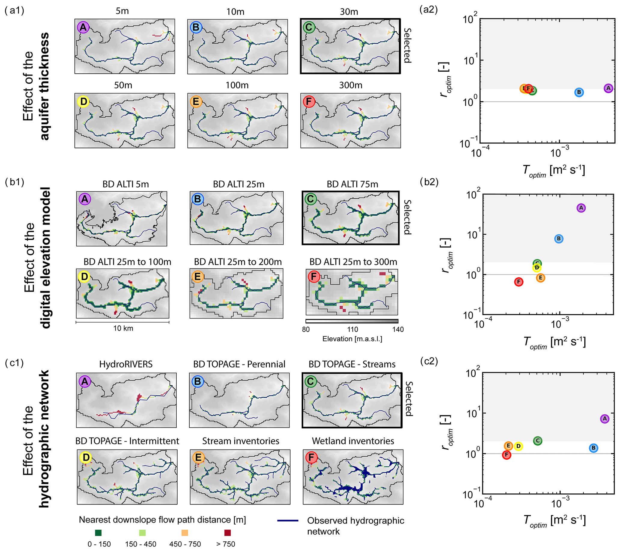
Figure 5Sensitivity analysis of the method for the Canut catchment (site 6) to (a) the DEM resolution, (b) the density and extent of the steam network displayed by different stream network products, and (c) the aquifer thickness. Panels (a1, b1, c1) show the downslope flow path distances of the simulated stream pixels projected onto the observed reference stream network for . Panels (a2, b2, c2) show roptim as a function of Toptim.
We also investigate the sensitivity of the resolutions of both the DEM (Fig. 5b) and the observed stream network (Fig. 5c) to the estimations of Toptim. The resolution of the DEM has only a minor influence on the estimation of optimal transmissivity, while the resolution of the stream network has a major impact. Figure 5b1 shows that the simulated stream network corresponds well to the observed network for the different DEM resolutions. However, the estimated optimal transmissivities vary significantly across the different cases (Fig. 5b2). For cases C, D and E, the estimated Toptim values remain close to each other, ranging from to m2 s−1. For case F, Toptim reaches a value of m2 s−1, while for A and B, it takes values of and m2 s−1, respectively. For cases C to F, the roptim criterion (Eq. 3) remains close to 1 (from 0.5 to 1.8), smaller than the threshold of 2 (Eq. 4). However, for the 5 and 25 m resolutions tested (cases A and B), the distances and are highly sensitive to the mismatch between an increasingly accurate DEM and a coarsely defined stream network. The main factor driving and is no longer the hydraulic conductivity but the mismatch between the DEM and the observed stream network, with roptim values becoming larger (respectively, 46.5 and 7.7 for the 5 and 25 m resolutions tested). These results emphasize that DEMs with resolutions that are too fine, here 5 and 25 m, cannot be used with the observed stream network selected in this study, at least at the current stage of the methodological development. Resolutions of 75 m and coarser, however, lead to consistent estimations of the hydraulic conductivity confirming the validity of the modeling approach.
We have systematically tested the method using six different stream network products issued by global, national and local databases (Fig. 5c1). These products display important differences in the extent and densities of the stream network coming from their origin and scale of observations (Appendix A). For case A, the global-scale product HydroRIVERS (Lehner et al., 2013) locates rivers away from the topographic valleys of the DEM, with consequently a Doptim value more than 10 times larger than DEMres. For cases B to F, the criterion roptim (Eq. 3) remains smaller than 2, the hydrographic network is well captured and the method estimates Toptim consistently (Fig. 5c2). Toptim varies over 1 order of magnitude from 2.0 x 10⁻⁴ to m2 s−1 and logically tends to decrease when the density and extent of the mapped stream network increases. Indeed, for a fixed recharge rate, lower transmissivities raise the groundwater table and broaden the headwater streams (Fig. 5c, E and F). Conversely, higher values of T contract the hydrographic networks with streams located mainly at lower elevations (Fig. 5c1, A and B). The extent of the stream system and the first-order stream locations appear to be highly sensitive to the estimated transmissivity confirming its capacity to inform the hydraulic conductivity.
3.2 Application to the ensemble of catchments
The method has been applied to the 23 other catchments (Fig. 3) with the same DEM resolution of 75 m, the product for the observed reference stream network and an aquifer thickness of 30 m. Both and were found to systematically intersect defining optimal Doptim (Fig. 6) and values (Table 1). For 19 sites, the value of Doptim is less than 2 pixels (Fig. 6), showing good consistency between the simulated and the observed stream network, and varies between 1397 to 19 687. Considering dsat computed by the model, Toptim values range over 1 order of magnitude from to m2 s−1 (Fig. 6), resulting in Koptim values between and m s−1 (Table 1). The model captures correctly the features of the observed stream network even in the presence of singular topographical features such as extended depressions or sharp changes in slope (Gauvain et al., 2021; Schumm et al., 1995). This is especially the case at site 7 where the seepage along the foot slope issued by a steep slope transition (6 % on 1000 m of length) located along a lithological contact is well represented both by the model and in the observations as a significant and perennial groundwater spring and/or wetland (Vautier et al., 2019; Kolbe et al., 2016).
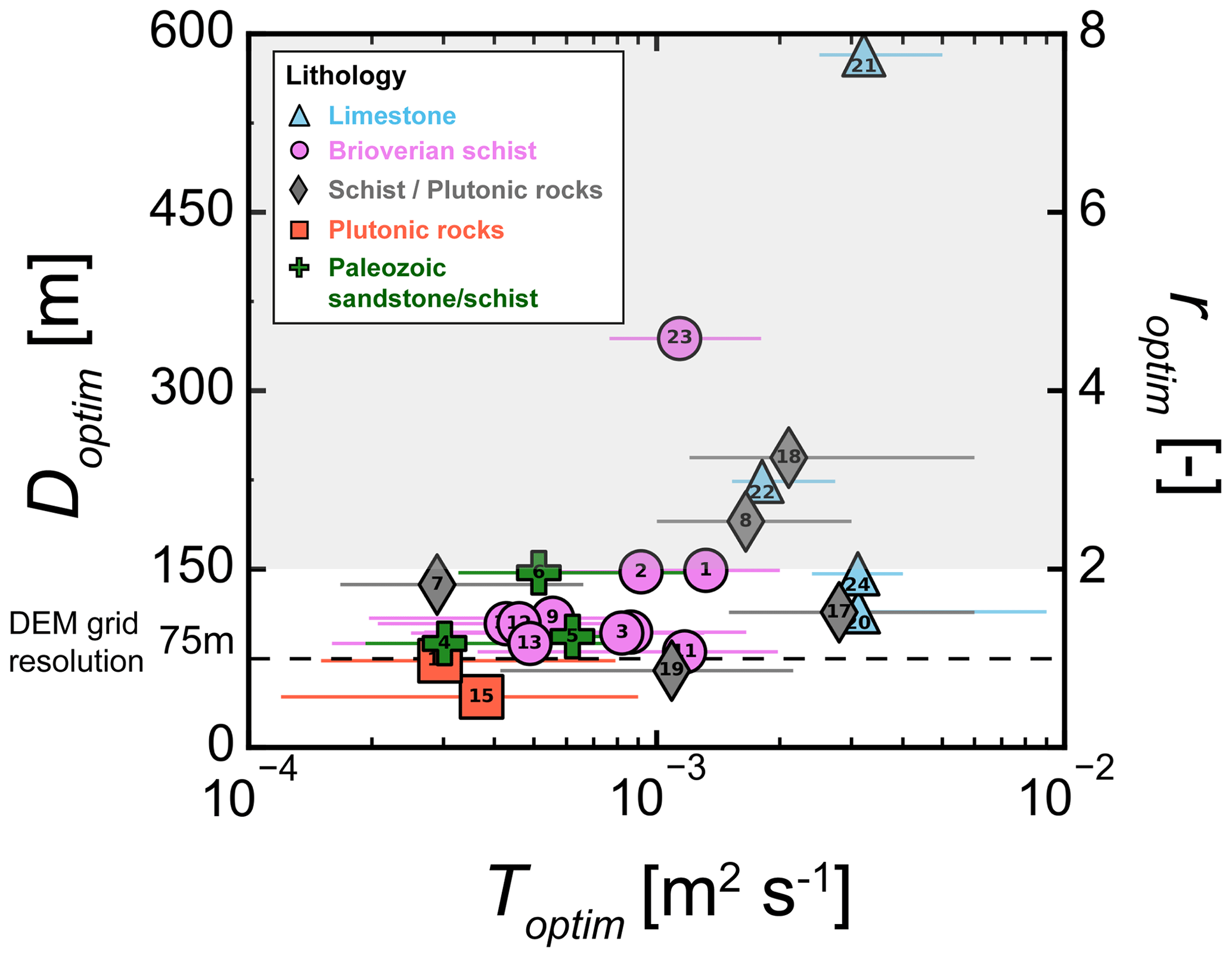
Figure 6Doptim and roptim criteria as functions of Toptim estimated for the 24 sites. The optimal transmissivity Toptim is obtained by considering Koptim, and the mean saturated aquifer thickness dsat is computed. The shaded area corresponds to sites with roptim>2. The DEM resolution is 75 m and the aquifer thickness is 30 m. The error bars correspond to the estimated Toptim considering the DEM resolution as an uncertainty indicator.
4.1 A new calibration method for the assessment of effective catchment-scale hydraulic properties
We have presented a process-based groundwater modeling approach to assess effective catchment-scale hydraulic properties (K and T) from the sole information on the density and spatial extent of the stream network. The proposed method (1) simulates the stream network by physically representing the 3D groundwater flows, (2) quantifies the mismatch between observed and simulated stream networks through distance-based spatial indicators and (3) calibrates the subsurface hydraulic properties by minimizing a performance criterion. We compare it with existing approaches and indicators.
Previous modeling approaches were mostly based on TOPMODEL applications (Blazkova et al., 2002; Güntner et al., 2004; Franks et al., 1998) or hillslope-scale flows (Luo et al., 2010). They had the advantage of simplicity but were limited in simple cases where flows are topography-driven. Like the 1D hillslope-scale approach of Stoll and Weiler (2010), our 3D distributed- and process-based groundwater approach remains valid in conditions where the groundwater table is not a strict replicate of the topography becoming “recharge controlled” (Haitjema and Mitchell-Bruker, 2005). It also accounts for the discontinuities of the seepage structure coming from the irregular connections of the subsurface flows with the surface (Godsey and Kirchner, 2014; Whiting and Godsey, 2016; Warix et al., 2021). It follows numerous field observations and synthetic experiments showing the strong influence of 3D groundwater flow organizations on the location of seepage zones (Goderniaux et al., 2013; Fleckenstein et al., 2006; Gauvain et al., 2021; Dohman et al., 2021).
Several indicators have been proposed to compare the spatial patterns of the modeled and observed saturated areas mostly based on cell-by-cell and cell–neighborhood approaches. This includes the likelihood measure (Franks et al., 1998; Blazkova et al., 2002), the Kappa goodness-of-fit statistic (Stoll and Weiler, 2010) and the Euclidean distance between cells (Güntner et al., 2004). These indicators are essentially local and readily accessible from information on topography and stream networks. We propose more integrative indicators based on the distance between the observed and simulated stream networks computed along the steepest slope between them, as does the IDPR (Network Development and Persistence Index), to identify zones predominantly favorable to infiltration or runoff (Mardhel et al., 2021). The advantages of this procedure are to account for the topographical structure within the definition of the distances and to constrain the comparison to the best compromise between the over- and undersaturation, mainly driven by and , respectively.
4.2 Comparison of estimated hydraulic conductivities with previously published values
As shown in Fig. 6, the method predicts a distribution of T values that stands within 1 order of magnitude despite the broad range of lithological units investigated. Overall, our estimates of hydraulic properties are consistent with values found in previous studies conducted for similar sites and lithologic settings (Roques et al., 2016; Mougin et al., 2008; Dewandel et al., 2021; Cornette et al., 2022; Leray et al., 2012). We compared the estimated hydraulic conductivity, Koptim, with local to regional values found in the literature Kliterature (Fig. 7). We focused on the comparison with local estimates from hydraulic tests or numerical groundwater models for two of the studied sites (Le Borgne et al., 2006; Kolbe et al., 2016; Jiménez-Martínez et al., 2013) or on those compiled in regional syntheses according to the lithology (Laurent et al., 2017; BRGM, 2018). Figure 7 shows a good agreement between our results and the other values. More specifically, the local values extracted for catchments 7 and 19 slightly underestimate the one from the literature by about 33 % (Fig. 7, diamonds). The hydraulic conductivities derived from regional synthesis remain within the same order of magnitude with a limited overestimation of a factor of 2 (Fig. 7, circles). This slight overestimation might result from testing methods as well as the fact that local hydraulic tests are often carried out close to transmissive geological features of major interest for water supply. Our results were also compared to those compiled in the global-scale database GLHYMPS (Huscroft et al., 2018). From the database, we derived equivalent hydraulic conductivities for each of the catchments. They range over 4 orders of magnitude, systematically lower by 1 to several orders of magnitude than our estimates (Appendix C). As shown in previous studies (de Graaf et al., 2020; Tashie et al., 2021), we find that the hydraulic conductivity dataset compiled in GLHYMPS may be locally underestimated.
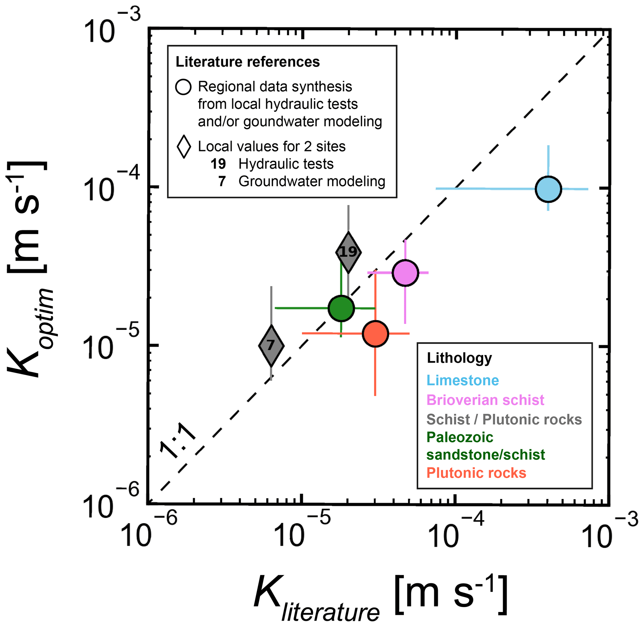
Figure 7Comparison of Koptim obtained for the 24 catchments with values found in the literature Kliterature grouped into two categories according to the scale of investigation (local vs. regional). Diamonds: values from hydraulic tests and/or groundwater modeling compiled in regional syntheses according to lithologies (BRGM, 2018; Laurent et al., 2017). Circles: K obtained from local hydraulic tests for site 19 (Le Borgne et al., 2006; Jiménez-Martínez et al., 2013) and groundwater modeling for site 7 (Kolbe et al., 2016). The values provided in transmissivity by the literature are translated into hydraulic conductivities by applying the same aquifer thickness of 30 m.
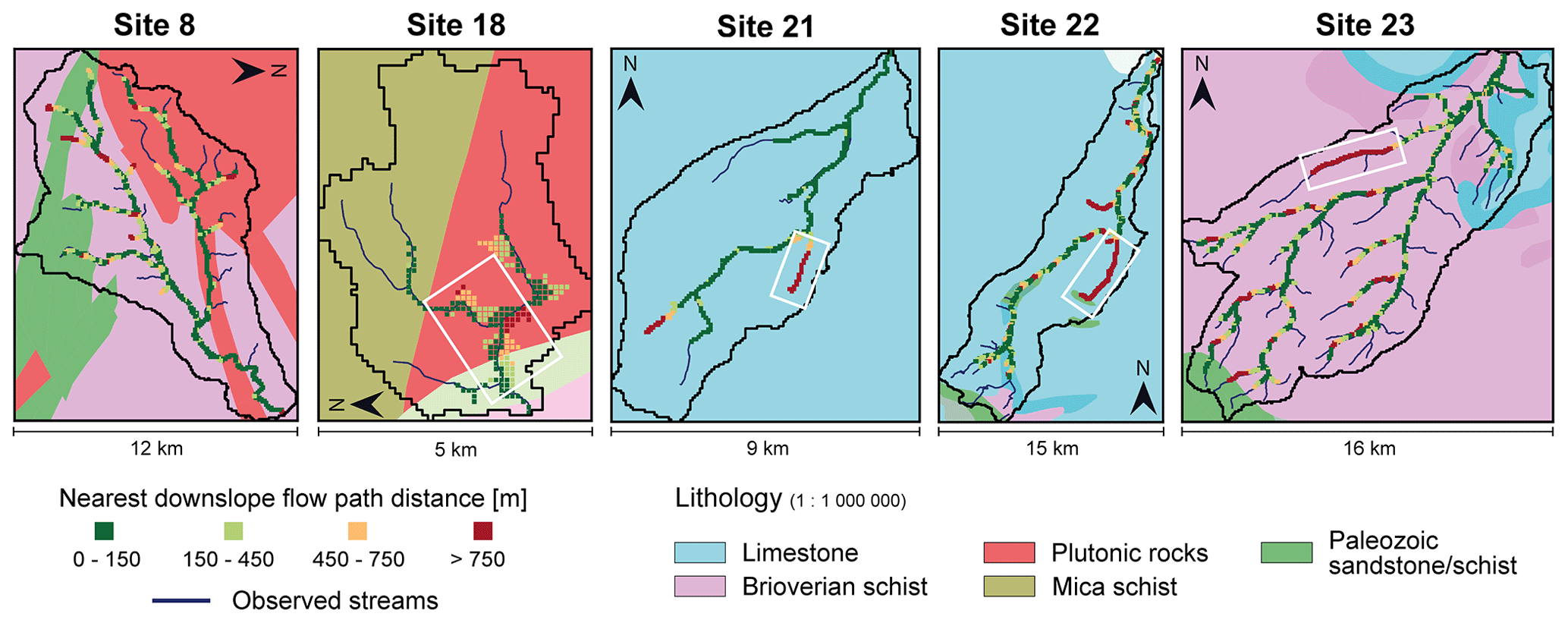
Figure 8For the five sites corresponding to roptim>2, representation of the observed stream network on top of the simplified geological map (1:1 000 000 scale), with the downslope flow path distances of the simulated seepage areas projected to the observed streams. For site 8, differences are larger on the plutonic rocks. For the other sites, the white square identifies the area where differences are the largest.
The results also show a range of values consistent with those given by classical textbooks for the investigated lithologies (Freeze and Cherry, 1979; Domenico and Schwartz, 1990). Crystalline rocks characterized by weathering and fractures (Roques et al., 2014; Dewandel et al., 2006) have a lower hydraulic conductivity than sedimentary rocks, here represented by limestones with a karstic systems (IGN and OFB, 2019) that, as expected, display higher conductivities. Lower conductivities suggest a high water table inducing a larger spatial extent of the stream network, confirmed by local knowledge, with a much higher observed drainage density for crystalline sites compared to limestone sites (Table 1). Although our results show evidence that effective conductivities are related to variations in dominant lithologies, it is also clear that other reported factors like erosion, bedrock weathering and fracturing may tend to homogenize the hydraulic properties in similar erosion and/or weathering settings (Luo et al., 2016; Yoshida and Troch, 2016; Jefferson et al., 2010; Litwin et al., 2022).
4.3 Sensitivity to input and/or model parameters: related improvements for broader applicability
The Doptim indicator (Eq. 2) provides information on the level of uncertainty. It depends on the quality of the data (observed reference stream network and the DEM) and on the model assumptions. Five sites (8, 18, 21, 22 and 23) over the 23 sites studied display a low match between the simulated and observed stream networks (roptim>2), with Doptim values ranging from 190 to 581 m (Fig. 6). Figure 8 maps the simulation results for these five sites. For site 18, the model predicts a seepage zone induced by a topographic depression representing potential ponds, lakes and wetlands, which are not in the observations. For sites 21 and 22, the main differences are located at a non-reported subsurface flow in the observed stream network within a karstic system (IGN and OFB, 2019); however, this is represented well by the model due to a topographic depression along this area. For site 23, the simulated flow at the bottom of the DEM valley appears to be parallel to the observed flow. In this case, it seems to be a registration error in the alignment of the stream location data within the DEM. For site 8, differences come principally from the model and, more specifically, from the assumption of a uniform hydraulic conductivity. For this site with lateral lithologic heterogeneity, we found that the model underestimates the extent and density of the stream network in the part with dominant plutonic rocks and overestimates them in the schists. At site 8, the IDPR (Mardhel et al., 2021) indicates that the granitic area is less permeable than the schist area and generally displays the limestone sites 21 and 22 primarily dominated by infiltration, consistent with our results.
The high sensitivity of applied to both the density and spatial extent of the observed stream network highlights the requirement of using high-quality stream products. Several issues may arise. First, river maps available in national to global databases are often incomplete compared to local databases compiled by stakeholders in direct field observations, leading to an overestimation of the effective hydraulic properties. Second, artificial channels, drainage ditches and any other departure from the geomorphic equilibrium may alter the stream network system and lead to an overestimation of the hydraulic properties in highly impacted zones. Third, the resolution of the DEM and reference stream network must be close. Nevertheless, the observed stream network layer could be adjusted to better match the DEM resolution.
Major limitations and improvements may also arise from the assumptions of the hydrogeological model. The proposed methodology can be used with other parameterizations and model conceptualizations. The model domain can be extended and the boundary conditions modified to better represent potentially longer and deeper regional groundwater circulations. If the information is available, the method could be tested with heterogeneous recharge at the catchment scale. The geometry of the aquifer could be adapted, applying flat- or irregular-bottom aquifers based on geophysical measurements (Pasquet et al., 2022) or depth to bedrock databases (Shangguan et al., 2017; Hengl et al., 2017; Pelletier et al., 2016). Exponentially decreasing conductivity with depth can be applied to the model in order to estimate the initial value of K at the surface or its characteristic decay depth. At the current stage of the method, catchment-scale lithological heterogeneities can be considered by applying the methodology independently on sub-areas characterized by a homogeneous lithology. For example, at the studied site 8, the application of the methodology on granite-dominated sub-catchments should result in lower K estimates than in the schist areas. Localized heterogeneities including weathering, fractures, faults and other discontinuities cannot be identified. They should be explicitly introduced into the model and characterized by other methods.
Global syntheses compiling accurate predictions of hydraulic properties of the subsurface are critically needed to predict water resource availabilities (Fan et al., 2019) in ungauged catchments (Sivapalan et al., 2003; Hrachowitz et al., 2013) and to assess the impact of hillslope- and catchment-scale hydrology on global change predictions (Taylor et al., 2013). Besides the climatic forcing data, requiring only a stream network map to calibrate a groundwater flow model built from a DEM, the approach presented in this article addresses this challenge, specifically for ungauged basins. Under the assumption that the transmissivity (hydraulic conductivity integrated over the saturated aquifer thickness) controls the extension and density of the hydrographic network, the approach calibrates the effective hydraulic properties against the stream network. The resolution of the stream network and DEM should be consistent. We showed that the spatialized performance criterion based on the distances between the simulated and observed stream network achieves an equilibrium between over- and undersaturation of the underlying groundwater system, as well as an equilibrium between over- and underestimation of the stream network extent. The resulting estimated K values are consistent with local values found in the literature.
A major advantage is the ease of deployment and transferability of the methodology to other catchments. Although the proposed methodology is limited to unconfined aquifers and particularly suited to contexts with significant subsurface–surface interactions, where groundwater primarily feeds streams, it aims to be deployed at multiple spatial scales by taking advantage of databases compiling topographic, hydrologic and climate information. Such deployment improving subsurface characterization from surface information would leverage the current development in crowdsourcing (Etter et al., 2020) and innovations in remote sensing (Biancamaria et al., 2016) that now provide high-resolution surface DEM products (Hawker et al., 2022; Yamazaki et al., 2017) and mapping of hydrographic networks (Grill et al., 2019; Yamazaki et al., 2019) distinguishing the perennial and intermittent streams (Fovet et al., 2021; Messager et al., 2021).
A1 Global database
HydroRIVERS (available on this website: https://www.hydrosheds.org/page/hydrorivers, last access: 1 September 2023) (Linke et al., 2019) is derived from HydroSHEDS (Lehner et al., 2013), a mapping product that provides stream information for regional- and global-scale applications, based on a grid resolution of 15 arcsec (approximately 500 m at the Equator).
A2 National database
The BD TOPAGE (available on this website: https://bdtopage.eaufrance.fr, last access: 1 September 2023) database classifies streams as perennial or intermittent based on historical photogrammetric reconstructions.
A3 Local database
The local stream and wetland inventory maps are based on observations and field surveys validated by the “Schéma d'Aménagement et de Gestion des Eaux” (SAGE) (available on this website: https://sdage-sage.eau-loire-bretagne.fr/home.html, last access: 1 September 2023).
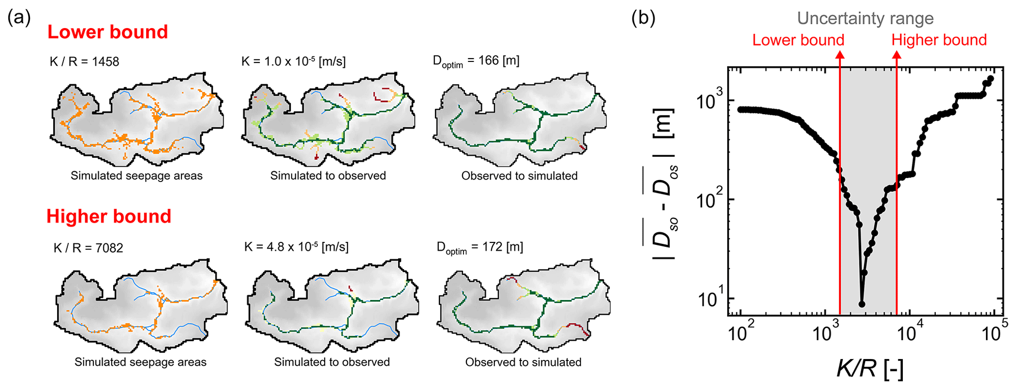
Figure B1For the Canut catchment (site 6), (a) 2D map views of simulated seepage areas and nearest downslope flow path distances (simulated to observed and observed to simulated) for the two values at the bounds of the uncertainty (lower and higher) and (b) the objective function based on the developed performance criteria obtained.
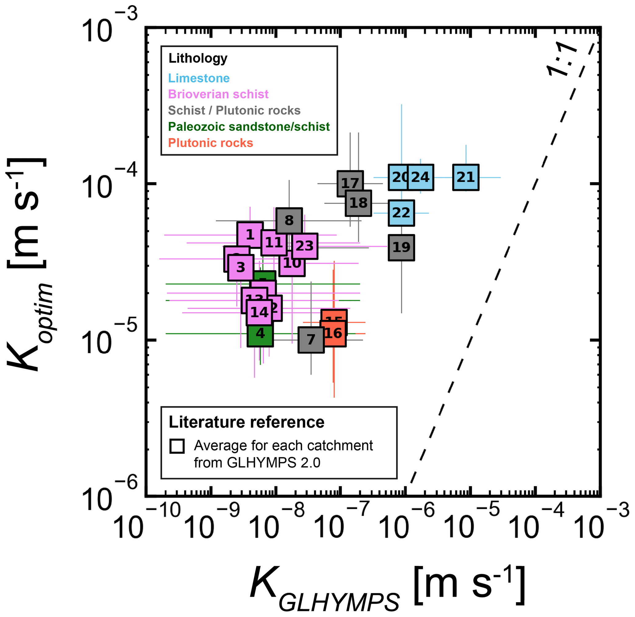
Figure C1Comparison of Koptim obtained for the 24 catchments with values from the literature, KGLHYMPS, provided by the GLHYMPS 2.0 global permeability map (Huscroft et al., 2018) and averaged over each catchment.
A Python code to test the method is available online in a shared repository: https://doi.org/10.5281/zenodo.8311547 (Abhervé, 2023).
The supplement related to this article is available online at: https://doi.org/10.5194/hess-27-3221-2023-supplement.
All co-authors were involved in the conceptualization of the original methods, identification of the research questions and the interpretation of the results. RA and AG developed the model, performed the simulations and analyzed the results. RA created the figures and prepared the first draft of the manuscript. All co-authors reviewed and edited the paper.
The contact author has declared that none of the authors has any competing interests.
Publisher's note: Copernicus Publications remains neutral with regard to jurisdictional claims in published maps and institutional affiliations.
Clément Roques acknowledges financial supports from the Rennes Métropole research chair “Ressource en Eau du Futur” and the European project WATERLINE (project ID CHIST-ERA-19-CES-006). Alexandre Gauvain acknowledges funding from the RIVAGES Normands 2100 project. The investigations also benefited from the support of the Network of hydrogeological research sites (H+) observatory and the French research observatory network of Critical Zone Observatories: Research and Applications (OZCAR-RI).
This work was funded by Eau du Bassin Rennais and Rennes Métropole, through the “Eaux et Territoires” (“Water and Territories”) research chairs of the Foundation of the University of Rennes (Fondation Rennes 1).
This paper was edited by Markus Weiler and reviewed by Ciaran Harman and one anonymous referee.
Abhervé, R.: Python code to test the calibration method of a groundwater flow model using a stream network, Zenodo [code], https://doi.org/10.5281/zenodo.8311547, 2023.
Achtziger-Zupančič, P., Loew, S., and Mariéthoz, G.: A new global database to improve predictions of permeability distribution in crystalline rocks at site scale, J. Geophys. Res.-Solid, 122, 3513–3539, https://doi.org/10.1002/2017JB014106, 2017.
Alley, W. M., Healy, R. W., LaBaugh, J. W., and Reilly, T. E.: Flow and storage in groundwater systems, Science, 296, 1985–1990, https://doi.org/10.1126/science.1067123, 2002.
Anderson, M. P., Woessner, W. W., and Hunt, R. J.: Applied groundwater modeling: simulation of flow and advective transport, in: 2nd Edn., Elsevier, AP Academic press is an imprint of Elsevier, Amsterdam, 564 pp., https://doi.org/10.1016/C2009-0-21563-7, 2015.
Bakker, M., Post, V., Langevin, C. D., Hughes, J. D., White, J. T., Starn, J. J., and Fienen, M. N.: Scripting MODFLOW Model Development Using Python and FloPy, Groundwater, 54, 733–739, https://doi.org/10.1111/gwat.12413, 2016.
Barclay, J. R., Starn, J. J., Briggs, M. A., and Helton, A. M.: Improved Prediction of Management-Relevant Groundwater Discharge Characteristics Throughout River Networks, Water Resour. Res., 56, 1–19, https://doi.org/10.1029/2020WR028027, 2020.
Beven, K., Asadullah, A., Bates, P., Blyth, E., Chappell, N., Child, S., Cloke, H., Dadson, S., Everard, N., Fowler, H. J., Freer, J., Hannah, D. M., Heppell, K., Holden, J., Lamb, R., Lewis, H., Morgan, G., Parry, L., and Wagener, T.: Developing observational methods to drive future hydrological science: Can we make a start as a community?, Hydrol. Process., 34, 868–873, https://doi.org/10.1002/hyp.13622, 2020.
Beven, K. J. and Kirkby, M. J.: A physically based, variable contributing area model of basin hydrology, Hydrol. Sci. Bull., 24, 43–69, https://doi.org/10.1080/02626667909491834, 1979.
Biancamaria, S., Lettenmaier, D. P., and Pavelsky, T. M.: The SWOT Mission and Its Capabilities for Land Hydrology, Surv. Geophys., 37, 307–337, https://doi.org/10.1007/s10712-015-9346-y, 2016.
Blazkova, S., Beven, K. J., and Kulasova, A.: On constraining TOPMODEL hydrograph simulations using partial saturated area information, Hydrol. Process., 16, 441–458, https://doi.org/10.1002/hyp.331, 2002.
Blöschl, G., Bierkens, M. F. P., Chambel, A., et al.: Twenty-three unsolved problems in hydrology (UPH) – a community perspective, Hydrolog. Sci. J., 64, 1141–1158, https://doi.org/10.1080/02626667.2019.1620507, 2019.
Bravo, H. R., Jiang, F., and Hunt, R. J.: Using groundwater temperature data to constrain parameter estimation in a groundwater flow model of a wetland system, Water Resour. Res., 38, 28-1–28-14, https://doi.org/10.1029/2000wr000172, 2002.
Bresciani, E., Davy, P., and De Dreuzy, J. R.: Is the Dupuit assumption suitable for predicting the groundwater seepage area in hillslopes?, Water Resour. Res., 50, 2394–2406, https://doi.org/10.1002/2013WR014284, 2014.
BRGM: Tectonic-lithostratigraphic log with evolution of hydrodynamic parameters according to lithological sets, SIGES Bretagne – Système d'information pour la Gestion des eaux Souterraine en Bretagne, https://sigesbre.brgm.fr/Comparaison-des-parametres-hydrodynamiques-avec-les.html (last access: 1 September 2023), 2018.
Brutsaert, W. and Nieber, J. L.: Regionalized Drought Flow Hydrographs From a Mature Glaciated Plateau, Water Resour. Res., 13, 637–643, https://doi.org/10.1029/WR013i003p00637, 1977.
Burden, R. L. and Faires, J. D.: 2.1 The Bisection Algorithm, in: Numerical Analysis, 3rd Edn., PWS Publishers, ISBN 0-87150-857-5, 1985.
Carrera, J., Alcolea, A., Medina, A., Hidalgo, J., and Slooten, L. J.: Inverse problem in hydrogeology, Hydrogeol. J., 13, 206–222, https://doi.org/10.1007/s10040-004-0404-7, 2005.
Chow, R., Frind, M. E., Frind, E. O., Jones, J. P., Sousa, M. R., Rudolph, D. L., Molson, J. W., and Nowak, W.: Delineating baseflow contribution areas for streams – A model and methods comparison, J. Contam. Hydrol., 195, 11–22, https://doi.org/10.1016/j.jconhyd.2016.11.001, 2016.
Comunian, A. and Renard, P.: Introducing wwhypda: A world-wide collaborative hydrogeological parameters database, Hydrogeol. J., 17, 481–489, https://doi.org/10.1007/s10040-008-0387-x, 2009.
Cornette, N., Roques, C., Boisson, A., Courtois, Q., Marçais, J., Launay, J., Pajot, G., Habets, F., and de Dreuzy, J. R.: Hillslope-scale exploration of the relative contribution of base flow, seepage flow and overland flow to streamflow dynamics, J. Hydrol., 610, 127992, https://doi.org/10.1016/j.jhydrol.2022.127992, 2022.
Cromwell, E., Shuai, P., Jiang, P., Coon, E. T., Painter, S. L., Moulton, J. D., Lin, Y., and Chen, X.: Estimating Watershed Subsurface Permeability From Stream Discharge Data Using Deep Neural Networks, Front. Earth Sci., 9, 1–13, https://doi.org/10.3389/feart.2021.613011, 2021.
Cuthbert, M. O., Gleeson, T., Moosdorf, N., Befus, K. M., Schneider, A., Hartmann, J., and Lehner, B.: Global patterns and dynamics of climate–groundwater interactions, Nat. Clim. Change, 9, 137–141, https://doi.org/10.1038/s41558-018-0386-4, 2019.
Day, D. G.: Lithologic controls of drainage density: a stud of six small rural catchments in New England, N.S.W., CATENA, 7, 339–351, 1980.
de Graaf, I., Condon, L., and Maxwell, R.: Hyper-Resolution Continental-Scale 3-D Aquifer Parameterization for Groundwater Modeling, Water Resour. Res., 56, 1–14, https://doi.org/10.1029/2019WR026004, 2020.
Dembélé, M., Hrachowitz, M., Savenije, H. H. G., Mariéthoz, G., and Schaefli, B.: Improving the Predictive Skill of a Distributed Hydrological Model by Calibration on Spatial Patterns With Multiple Satellite Data Sets, Water Resour. Res., 56, 1–26, https://doi.org/10.1029/2019WR026085, 2020.
Devauchelle, O., Petroff, A. P., Seybold, H. F., and Rothman, D. H.: Ramification of stream networks, P. Natl. Acad. Sci. USA, 109, 20832–20836, https://doi.org/10.1073/pnas.1215218109, 2012.
De Vries, J. J.: Dynamics of the interface between streams and groundwater systems in lowland areas, with reference to stream net evolution, J. Hydrol., 155, 39–56, https://doi.org/10.1016/0022-1694(94)90157-0, 1994.
Dewandel, B., Lachassagne, P., Wyns, R., Maréchal, J. C., and Krishnamurthy, N. S.: A generalized 3-D geological and hydrogeological conceptual model of granite aquifers controlled by single or multiphase weathering, J. Hydrol., 330, 260–284, https://doi.org/10.1016/j.jhydrol.2006.03.026, 2006.
Dewandel, B., Boisson, A., Amraoui, N., Caballero, Y., Mougin, B., Baltassat, J. M., and Maréchal, J. C.: Improving our ability to model crystalline aquifers using field data combined with a regionalized approach for estimating the hydraulic conductivity field, J. Hydrol., 601, 126652, https://doi.org/10.1016/j.jhydrol.2021.126652, 2021.
Dietrich, W. E. and Dunne, T.: The Channel Head, in: Channel Network Hydrology, edited by: Beven, K. and Kirkby, M. J., Wiley, New York, 175–219, 1993.
Dohman, J. M., Godsey, S. E., and Hale, R. L.: Three-Dimensional Subsurface Flow Path Controls on Flow Permanence, Water Resour. Res., 57, 1–18, https://doi.org/10.1029/2020WR028270, 2021.
Domenico, P. A. and Schwartz, F. W.: Physical and Chemical Hydrogeology, 2nd Edn., John Wiley & Sons, Inc., ISBN 978-0-471-59762-9, 1990.
Dunne, T.: Formation and controls of channel networks, Prog. Phys. Geogr., 4, 211–239, https://doi.org/10.1177/030913338000400204, 1975.
Eckhardt, K. and Ulbrich, U.: Potential impacts of climate change on groundwater recharge and streamflow in a central European low mountain range, J. Hydrol., 284, 244–252, https://doi.org/10.1016/j.jhydrol.2003.08.005, 2003.
Elshall, A. S., Arik, A. D., El-Kadi, A. I., Pierce, S., Ye, M., Burnett, K. M., Wada, C. A., Bremer, L. L., and Chun, G.: Groundwater sustainability: a review of the interactions between science and policy, Environ. Res. Lett., 15, 093004, https://doi.org/10.1088/1748-9326/ab8e8c, 2020.
Etter, S., Strobl, B., Seibert, J., and van Meerveld, H. J. I.: Value of Crowd-Based Water Level Class Observations for Hydrological Model Calibration, Water Resour. Res., 56, 1–17, https://doi.org/10.1029/2019WR026108, 2020.
Fan, Y.: Groundwater in the Earth's critical zone: Relevance to large-scale patterns and processes, Water Resour. Res., 51, 3052–3069, https://doi.org/10.1002/2015WR017037, 2015.
Fan, Y., Li, H., and Miguez-Macho, G.: Global Patterns of Groundwater Table Depth, Science, 339, 940–943, https://doi.org/10.1126/science.1229881, 2013.
Fan, Y., Richard, S., Bristol, R. S., Peters, S. E., Ingebritsen, S. E., Moosdorf, N., Packman, A., Gleeson, T., Zaslavsky, I., Peckham, S., Murdoch, L., Fienen, M., Cardiff, M., Tarboton, D., Jones, N., Hooper, R., Arrigo, J., Gochis, D., Olson, J., and Wolock, D.: DigitalCrust – a 4D data system of material properties for transforming research on crustal fluid flow, Geofluids, 15, 372–379, https://doi.org/10.1111/gfl.12114, 2015.
Fan, Y., Clark, M., Lawrence, D. M., Swenson, S., Band, L. E., Brantley, S. L., Brooks, P. D., Dietrich, W. E., Flores, A., Grant, G., Kirchner, J. W., Mackay, D. S., McDonnell, J. J., Milly, P. C. D., Sullivan, P. L., Tague, C., Ajami, H., Chaney, N., Hartmann, A., Hazenberg, P., McNamara, J., Pelletier, J., Perket, J., Rouholahnejad-Freund, E., Wagener, T., Zeng, X., Beighley, E., Buzan, J., Huang, M., Livneh, B., Mohanty, B. P., Nijssen, B., Safeeq, M., Shen, C., van Verseveld, W., Volk, J., and Yamazaki, D.: Hillslope Hydrology in Global Change Research and Earth System Modeling, Water Resour. Res., 55, 1737–1772, https://doi.org/10.1029/2018WR023903, 2019.
Fleckenstein, J. H., Niswonger, R. G., and Fogg, G. E.: River-aquifer interactions, geologic heterogeneity, and low-flow management, Ground Water, 44, 837–852, https://doi.org/10.1111/j.1745-6584.2006.00190.x, 2006.
Fovet, O., Belemtougri, A., Boithias, L., Marylise, J. C., Kevin, C., and Braud, I.: Intermittent rivers and ephemeral streams: Perspectives for critical zone science and research on socio-ecosystems, 8, 1–33, https://doi.org/10.1002/wat2.1523, 2021.
Franks, S. W., Gineste, P., Beven, K. J., and Merot, P.: On constraining the predictions of a distributed model: The incorporation of fuzzy estimates of saturated areas into the calibration process, Water Resour. Res., 34, 787–797, https://doi.org/10.1029/97WR03041, 1998.
Freeze, R. A. and Cherry, J. A.: Groundwater, edited by: Prentice-Hall, Englewood Cliffs, NJ, 604 pp., ISBN 978-0133653120, 1979.
Gauvain, A., Leray, S., Marçais, J., and Roques, C.: Geomorphological Controls on Groundwater Transit Times: A Synthetic Analysis at the Hillslope Scale, Water Resour. Res., 57, e2020WR029463, https://doi.org/10.1029/2020WR029463, 2021.
Gleeson, T. and Manning, A. H.: Regional groundwater flow in mountainous terrain: Three-dimensional simulations of topographic and hydrogeologic controls, Water Resour. Res., 44, W10403, https://doi.org/10.1029/2008WR006848, 2008.
Gleeson, T., Moosdorf, N., Hartmann, J., and van Beek, L. P. H.: A glimpse beneath earth's surface: GLobal HYdrogeology MaPS (GLHYMPS) of permeability and porosity, Geophys. Res. Lett., 41, 3891–3898, https://doi.org/10.1002/2014GL059856, 2014.
Gleeson, T., Wagener, T., Döll, P., Zipper, S. C., West, C., Wada, Y., Taylor, R., Scanlon, B., Rosolem, R., Rahman, S., Oshinlaja, N., Maxwell, R., Lo, M. H., Kim, H., Hill, M., Hartmann, A., Fogg, G., Famiglietti, J. S., Ducharne, A., De Graaf, I., Cuthbert, M., Condon, L., Bresciani, E., and Bierkens, M. F. P.: GMD perspective: The quest to improve the evaluation of groundwater representation in continental-to global-scale models, Geosci. Model Dev., 14, 7545–7571, https://doi.org/10.5194/gmd-14-7545-2021, 2021.
Goderniaux, P., Davy, P., Bresciani, E., de Dreuzy, J. R., and Le Borgne, T.: Partitioning a regional groundwater flow system into shallow local and deep regional flow compartments, Water Resour. Res., 49, 2274–2286, https://doi.org/10.1002/wrcr.20186, 2013.
Godsey, S. E. and Kirchner, J. W.: Dynamic, discontinuous stream networks: Hydrologically driven variations in active drainage density, flowing channels and stream order, Hydrol. Process., 28, 5791–5803, https://doi.org/10.1002/hyp.10310, 2014.
Grayson, R. B. and Blöschl, G. (Eds.): Spatial Patterns in Catchment Hydrology: Observations and Modelling, Cambridge University Press, Cambridge, UK, 404 pp., ISBN 0 521 63316 8, 2000.
Grill, G., Lehner, B., Thieme, M., Geenen, B., Tickner, D., Antonelli, F., Babu, S., Borrelli, P., Cheng, L., Crochetiere, H., Ehalt Macedo, H., Filgueiras, R., Goichot, M., Higgins, J., Hogan, Z., Lip, B., McClain, M. E., Meng, J., Mulligan, M., Nilsson, C., Olden, J. D., Opperman, J. J., Petry, P., Reidy Liermann, C., Sáenz, L., Salinas-Rodríguez, S., Schelle, P., Schmitt, R. J. P., Snider, J., Tan, F., Tockner, K., Valdujo, P. H., van Soesbergen, A., and Zarfl, C.: Mapping the world's free-flowing rivers, Nature, 569, 215–221, https://doi.org/10.1038/s41586-019-1111-9, 2019.
Güntner, A., Seibert, J., and Uhlenbrook, S.: Modeling spatial patterns of saturated areas: An evaluation of different terrain indices, Water Resour. Res., 40, 1–19, https://doi.org/10.1029/2003WR002864, 2004.
Haitjema, H. M. and Mitchell-Bruker, S.: Are water tables a subdued replica of the topography?, Ground Water, 43, 781–786, https://doi.org/10.1111/j.1745-6584.2005.00090.x, 2005.
Harbaugh, A. W.: MODFLOW-2005: the U.S. Geological Survey modular ground-water model–the ground-water flow process, Techniques and Methods, USGS, https://doi.org/10.3133/tm6A16, 2005.
Hartmann, J. and Moosdorf, N.: The new global lithological map database GLiM: A representation of rock properties at the Earth surface, Geochem. Geophy. Geosy., 13, 1–37, https://doi.org/10.1029/2012GC004370, 2012.
Hawker, L., Uhe, P., Paulo, L., Sosa, J., Savage, J., Sampson, C., and Neal, J.: A 30 m global map of elevation with forests and buildings removed, Environ. Res. Lett., 17, 024016, https://doi.org/10.1088/1748-9326/ac4d4f, 2022.
Hengl, T., De Jesus, J. M., Heuvelink, G. B. M., Gonzalez, M. R., Kilibarda, M., Blagotiæ, A., Shangguan, W., Wright, M. N., Geng, X., Bauer-Marschallinger, B., Guevara, M. A., Vargas, R., MacMillan, R. A., Batjes, N. H., Leenaars, J. G. B., Ribeiro, E., Wheeler, I., Mantel, S., and Kempen, B.: SoilGrids250m: Global gridded soil information based on machine learning, PLOS ONE, 12, e0169748, https://doi.org/10.1371/journal.pone.0169748, 2017.
Holman, I. P., Allen, D. M., Cuthbert, M. O., and Goderniaux, P.: Towards best practice for assessing the impacts of climate change on groundwater, Hydrogeol. J., 20, 1–4, https://doi.org/10.1007/s10040-011-0805-3, 2012.
Hrachowitz, M., Savenije, H. H. G., Blöschl, G., McDonnell, J. J., Sivapalan, M., Pomeroy, J. W., Arheimer, B., Blume, T., Clark, M. P., Ehret, U., Fenicia, F., Freer, J. E., Gelfan, A., Gupta, H. V., Hughes, D. A., Hut, R. W., Montanari, A., Pande, S., Tetzlaff, D., Troch, P. A., Uhlenbrook, S., Wagener, T., Winsemius, H. C., Woods, R. A., Zehe, E., and Cudennec, C.: A decade of Predictions in Ungauged Basins (PUB) – a review, Hydrolog. Sci. J., 58, 1198–1255, https://doi.org/10.1080/02626667.2013.803183, 2013.
Hsieh, P. A., Bredehoeft, J. D., and Farr, J. M.: Determination of aquifer transmissivity from Earth tide analysis, Water Resour. Res., 23, 1824–1832, https://doi.org/10.1029/WR023i010p01824, 1987.
Huscroft, J., Gleeson, T., Hartmann, J., and Börker, J.: Compiling and Mapping Global Permeability of the Unconsolidated and Consolidated Earth: GLobal HYdrogeology MaPS 2.0 (GLHYMPS 2.0), Geophys. Res. Lett., 45, 1897–1904, https://doi.org/10.1002/2017GL075860, 2018.
IGN: Le modèle numérique de terrain (MNT) maillé qui décrit le relief du territoire français à moyenne échelle BD ALTI® version 2021, Information Géographique sur l'Eau et Institut National de l'Information Géographique et Forestière [data set], https://geoservices.ign.fr/bdalti (last access: 1 September 2023), 2021.
IGN and OFB: Jeu de données des cours d'eau de France métropolitaine BD TOPAGE®version 2019, Office Français de la Biodiversité (OFB) – Information Géographique sur l'Eau et Institut National de l'Information Géographique et Forestière [data set], https://bdtopage.eaufrance.fr/ (last access: 1 September 2023), 2019.
Jefferson, A., Grant, G. E., Lewis, S. L., and Lancaster, S. T.: Coevolution of hydrology and topography on a basalt landscape in the Oregon Cascade Range, USA, Earth Surf. Proc. Land., 35, 803–816, https://doi.org/10.1002/esp.1976, 2010.
Jiménez-Martínez, J., Longuevergne, L., Le Borgne, T., Davy, P., Russian, A., and Bour, O.: Temporal and spatial scaling of hydraulic response to recharge in fractured aquifers: Insights from a frequency domain analysis, Water Resour. Res., 49, 3007–3023, https://doi.org/10.1002/wrcr.20260, 2013.
Kolbe, T., Marçais, J., Thomas, Z., Abbott, B. W., de Dreuzy, J.-R., Rousseau-Gueutin, P., Aquilina, L., Labasque, T., and Pinay, G.: Coupling 3D groundwater modeling with CFC-based age dating to classify local groundwater circulation in an unconfined crystalline aquifer, J. Hydrol., 543, 31–46, https://doi.org/10.1016/j.jhydrol.2016.05.020, 2016.
Kuang, X. and Jiao, J. J.: An integrated permeability-depth model for Earth's crust, Geophys. Res. Lett., 2, 7539–7545, https://doi.org/10.1002/2014GL061999, 2014.
Laurent, A., Le Cozannet, G., Couëffé, R., Schroetter, J.-M., Croiset, N., and Lions, J.: Vulnérabilité des aquifères côtiers face aux intrusions salines en Normandie occidentale, Rapp. Final BRGM/RP-66052-FR, 189 pp., BRGM, https://infoterre.brgm.fr/rapports/RP-66052-FR.pdf (last access: 1 September 2023), 2017.
Le Borgne, T., Bour, O., Paillet, F. L., and Caudal, J. P.: Assessment of preferential flow path connectivity and hydraulic properties at single-borehole and cross-borehole scales in a fractured aquifer, J. Hydrol., 328, 347–359, https://doi.org/10.1016/j.jhydrol.2005.12.029, 2006.
Lehner, B. and Grill, G.: Global river hydrography and network routing: Baseline data and new approaches to study the world's large river systems, Hydrol. Process., 27, 2171–2186, https://doi.org/10.1002/hyp.9740, 2013.
Lehner, B., Verdin, K., and Jarvis, A.: New global hydrography derived from spaceborne elevation data, T. EOS, 89, 93–94, 2013 (data available at: https://www.hydrosheds.org, last access: 1 September 2023)
Leibowitz, S. G., Wigington, P. J., Schofield, K. A., Alexander, L. C., Vanderhoof, M. K., and Golden, H. E.: Connectivity of Streams and Wetlands to Downstream Waters: An Integrated Systems Framework, J. Am. Water Resour. Assoc., 54, 298–322, https://doi.org/10.1111/1752-1688.12631, 2018.
Le Moine, N.: Le bassin versant de surface vu par le souterrain: une voie d’amélioration des performances et du réalisme des modèles pluie-débit?, Thèse de doctorat, Université Pierre et Marie Curie, 348 pp., 2008.
Le Moigne, P., Besson, F., Martin, E., Boé, J., Boone, A., Decharme, B., Etchevers, P., Faroux, S., Habets, F., Lafaysse, M., Leroux, D., and Rousset-Regimbeau, F.: The latest improvements with SURFEX v8.0 of the Safran–Isba–Modcou hydrometeorological model for France, Geosci. Model Dev., 13, 3925–3946, https://doi.org/10.5194/gmd-13-3925-2020, 2020.
Leray, S., de Dreuzy, J. R., Bour, O., Labasque, T., and Aquilina, L.: Contribution of age data to the characterization of complex aquifers, J. Hydrol., 464–465, 54–68, https://doi.org/10.1016/J.JHYDROL.2012.06.052, 2012.
Levizzani, V. and Cattani, E.: Satellite Remote Sensing of Precipitation and the Terrestrial Water Cycle in a Changing Climate, Remote Sens., 11, 2301, https://doi.org/10.3390/rs11192301, 2019.
Lindsay, J. B.: Whitebox GAT: A case study in geomorphometric analysis, Comput. Geosci., 95, 75–84, https://doi.org/10.1016/j.cageo.2016.07.003, 2016.
Linke, S., Lehner, B., Ouellet Dallaire, C., Ariwi, J., Grill, G., Anand, M., Beames, P., Burchard-Levine, V., Maxwell, S., Moidu, H., Tan, F., and Thieme, M.: Global hydro-environmental sub-basin and river reach characteristics at high spatial resolution, Sci. Data, 6, 1–16, https://doi.org/10.1038/s41597-019-0300-6, 2019.
Litwin, D. G., Tucker, G. E., Barnhart, K. R., and Harman, C. J.: Groundwater Affects the Geomorphic and Hydrologic Properties of Coevolved Landscapes, J. Geophys. Res.-Earth, 127, 1–36, https://doi.org/10.1029/2021JF006239, 2022.
Lovill, S. M., Hahm, W. J., and Dietrich, W. E.: Drainage from the Critical Zone: Lithologic Controls on the Persistence and Spatial Extent of Wetted Channels during the Summer Dry Season, Water Resour. Res., 54, 5702–5726, https://doi.org/10.1029/2017WR021903, 2018.
Luijendijk, E.: Transmissivity and groundwater flow exert a strong influence on drainage density, Earth Surf. Dynam., 10, 1–22, https://doi.org/10.5194/esurf-10-1-2022, 2022.
Luo, W. and Stepinski, T.: Identification of geologic contrasts from landscape dissection pattern: An application to the Cascade Range, Oregon, USA, Geomorphology, 99, 90–98, https://doi.org/10.1016/j.geomorph.2007.10.014, 2008.
Luo, W., Grudzinski, B. P., and Pederson, D.: Estimating hydraulic conductivity from drainage patterns – a case study in the Oregon Cascades, Geology, 38, 335–338, https://doi.org/10.1130/G30816.1, 2010.
Luo, W., Jasiewicz, J., Stepinski, T., Wang, J., Xu, C., and Cang, X.: Spatial association between dissection density and environmental factors over the entire conterminous United States, Geophys. Res. Lett., 43, 692–700, https://doi.org/10.1002/2015GL066941, 2016.
Marçais, J. and de Dreuzy, J. R.: Prospective Interest of Deep Learning for Hydrological Inference, Groundwater, 55, 688–692, https://doi.org/10.1111/gwat.12557, 2017.
Mardhel, V., Pinson, S., and Allier, D.: Description of an indirect method (IDPR) to determine spatial distribution of infiltration and runoff and its hydrogeological applications to the French territory, J. Hydrol., 592, 125609, https://doi.org/10.1016/j.jhydrol.2020.125609, 2021.
Mendoza, G. F., Steenhuis, T. S., Walter, M. T., and Parlange, J. Y.: Estimating basin-wide hydraulic parameters of a semi-arid mountainous watershed by recession-flow analysis, J. Hydrol., 279, 57–69, https://doi.org/10.1016/S0022-1694(03)00174-4, 2003.
Merot, P., Squividant, H., Aurousseau, P., Hefting, M., Burt, T., Maitre, V., Kruk, M., Butturini, A., Thenail, C., and Viaud, V.: Testing a climato-topographic index for predicting wetlands distribution along an European climate gradient, Ecol. Model., 163, 51–71, https://doi.org/10.1016/S0304-3800(02)00387-3, 2003.
Messager, M. L., Lehner, B., Cockburn, C., Lamouroux, N., Pella, H., Snelder, T., Tockner, K., Trautmann, T., Watt, C., and Datry, T.: Global prevalence of non-perennial rivers and streams, Nature, 594, 391–397, https://doi.org/10.1038/s41586-021-03565-5, 2021.
Mougin, B., Allier, D., Blanchin, R., Carn, A., Courtois, N., Gateau, C., and Putot, E.: SILURES Bretagne (Système d'Information pour la Localisation et l'Utilisation des Ressources en Eaux Souterraines), BRGM, http://infoterre.brgm.fr/rapports/RP-56457-FR.pdf (last access: 1 September 2023), 2008.
Niswonger, R. G., Panday, S., and Ibaraki, M.: MODFLOW-NWT, A Newton formulation for MODFLOW-2005: U.S. Geological Survey Techniques and Methods 6–A37, 44 pp., https://pubs.usgs.gov/tm/tm6a37/pdf/tm6a37.pdf (last access: 1 September 2023), 2011.
Noilhan, J. and Mahfouf, J. F.: The ISBA land surface parameterisation scheme, Global Planet. Change, 13, 145–159, https://doi.org/10.1016/0921-8181(95)00043-7, 1996.
Pasquet, S., Marçais, J., Hayes, J. L., Sak, P. B., Ma, L., and Gaillardet, J.: Catchment-scale architecture of the deep critical zone revealed by seismic imaging, Geophys. Res. Lett., 49, 1–13, https://doi.org/10.1029/2022gl098433, 2022.
Pederson, D. T.: Stream Piracy Revisited: A Groundwater-Sapping Solution, GSA Today, 4–10, https://doi.org/10.1130/1052-5173(2001)011<0004:SPRAGS>2.0.CO;2, 2001.
Pelletier, J. D., Broxton, P. D., Hazenberg, P., Zeng, X., Troch, P. A., Niu, G. Y., Williams, Z., Brunke, M. A., and Gochis, D.: A gridded global data set of soil, intact regolith, and sedimentary deposit thicknesses for regional and global land surface modeling, J. Adv. Model. Earth Syst., 8, 41–65, https://doi.org/10.1002/2015MS000526, 2016.
Prancevic, J. P. and Kirchner, J. W.: Topographic Controls on the Extension and Retraction of Flowing Streams, Geophys. Res. Lett., 46, 2084–2092, https://doi.org/10.1029/2018GL081799, 2019.
Quintana-Seguí, P., Le Moigne, P., Durand, Y., Martin, E., Habets, F., Baillon, M., Canellas, C., Franchisteguy, L., and Morel, S.: Analysis of near-surface atmospheric variables: Validation of the SAFRAN analysis over France, J. Appl. Meteorol. Clim., 47, 92–107, https://doi.org/10.1175/2007JAMC1636.1, 2008.
Ranjram, M., Gleeson, T., and Luijendijk, E.: Is the permeability of crystalline rock in the shallow crust related to depth, lithology or tectonic setting?, 15, 106–119, https://doi.org/10.1111/gfl.12098, 2015.
Rapinel, S., Panhelleux, L., Gayet, G., Vanacker, R., Lemercier, B., Laroche, B., Chambaud, F., Guelmami, A., and Hubert-Moy, L.: National wetland mapping using remote-sensing-derived environmental variables, archive field data, and artificial intelligence, Heliyon, 9, 1–17, https://doi.org/10.1016/j.heliyon.2023.e13482, 2023.
Refsgaard, J. C., Hojberg, A. L., Moller, I., Hansen, M., and Sondergaard, V.: Groundwater modeling in integrated water resources management – visions for 2020, Ground Water, 48, 633–648, https://doi.org/10.1111/j.1745-6584.2009.00634.x, 2010.
Reichstein, M., Camps-Valls, G., Stevens, B., Jung, M., Denzler, J., Carvalhais, N., and Prabhat: Deep learning and process understanding for data-driven Earth system science, Nature, 566, 195–204, 2019.
Renard, P.: The future of hydraulic tests, Hydrogeol. J., 13, 259–262, https://doi.org/10.1007/s10040-004-0406-5, 2005.
Roques, C., Aquilina, L., Bour, O., Maréchal, J. C., Dewandel, B., Pauwels, H., Labasque, T., Vergnaud-Ayraud, V., and Hochreutener, R.: Groundwater sources and geochemical processes in a crystalline fault aquifer, J. Hydrol., 519, 3110–3128, https://doi.org/10.1016/j.jhydrol.2014.10.052, 2014.
Roques, C., Bour, O., Aquilina, L., and Dewandel, B.: High-yielding aquifers in crystalline basement: insights about the role of fault zones, exemplified by Armorican Massif, France, Hydrogeol. J., 24, 2157–2170, https://doi.org/10.1007/s10040-016-1451-6, 2016.
Rotzoll, K. and El-Kadi, A. I.: Estimating hydraulic properties of coastal aquifers using wave setup, J. Hydrol., 353, 201–213, https://doi.org/10.1016/j.jhydrol.2008.02.005, 2008.
Schilling, O. S., Cook, P. G., and Brunner, P.: Beyond Classical Observations in Hydrogeology: The Advantages of Including Exchange Flux, Temperature, Tracer Concentration, Residence Time, and Soil Moisture Observations in Groundwater Model Calibration, Rev. Geophys., 57, 146–182, https://doi.org/10.1029/2018RG000619, 2019.
Schneider, A., Jost, A., Coulon, C., Silvestre, M., Théry, S., and Ducharne, A.: Global-scale river network extraction based on high-resolution topography and constrained by lithology, climate, slope, and observed drainage density, Geophys. Res. Lett., 44, 2773–2781, https://doi.org/10.1002/2016GL071844, 2017.
Schumm, S. A., Boyd, K. F., Wolff, C. G., and Spitz, W. J.: A ground-water sapping landscape in the Florida Panhandle, Geomorphology, 12, 281–297, 1995.
Shangguan, W., Hengl, T., Mendes de Jesus, J., Yuan, H., and Dai, Y.: Mapping the global depth to bedrock for land surface modeling, J. Adv. Model. Earth Syst., 9, 65–88, https://doi.org/10.1002/2016MS000686, 2017.
Sivapalan, M., Takeuchi, K., Franks, S. W., Gupta, V. K., Karambiri, H., Lakshmi, V., Liang, X., McDonnell, J. J., Mendiondo, E. M., O'Connell, P. E., Oki, T., Pomeroy, J. W., Schertzer, D., Uhlenbrook, S., and Zehe, E.: IAHS Decade on Predictions in Ungauged Basins (PUB), 2003-2012: Shaping an exciting future for the hydrological sciences, Hydrolog. Sci. J., 48, 857–880, https://doi.org/10.1623/hysj.48.6.857.51421, 2003.
Sophocleous, M.: Interactions between groundwater and surface water: the state of the science, Hydrogeol. J., 10, 52–67, https://doi.org/10.1007/s10040-001-0170-8, 2002.
Stoll, S. and Weiler, M.: Explicit simulations of stream networks to guide hydrological modelling in ungauged basins, Hydrol. Earth Syst. Sci., 14, 1435–1448, https://doi.org/10.5194/hess-14-1435-2010, 2010.
Strahler, A. N.: Quantitative geomorphology of drainage basins and channel networks, in: Handb. Appl. Hydrol., edited by: Chow, V. T., McGraw-Hill, New York, 439–476, 1964.
Tashie, A., Pavelsky, T. M., Band, L., and Topp, S.: Watershed-Scale Effective Hydraulic Properties of the Continental United States, J. Adv. Model. Earth Syst., 13, 1–18, https://doi.org/10.1029/2020MS002440, 2021.
Taylor, R. G., Scanlon, B., Doll, P., Rodell, M., van Beek, R., Wada, Y., Longuevergne, L., Leblanc, M., Famiglietti, J. S., Edmunds, M., Konikow, L., Green, T. R., Chen, J. Y., Taniguchi, M., Bierkens, M. F. P., MacDonald, A., Fan, Y., Maxwell, R. M., Yechieli, Y., Gurdak, J. J., Allen, D. M., Shamsudduha, M., Hiscock, K., Yeh, P. J. F., Holman, I., and Treidel, H.: Ground water and climate change, Nat. Clim. Change, 3, 322–329, https://doi.org/10.1038/nclimate1744, 2013.
Tootchi, A., Jost, A., and Ducharne, A.: Multi-source global wetland maps combining surface water imagery and groundwater constraints, Earth Syst. Sci. Data, 11, 189–220, https://doi.org/10.5194/essd-11-189-2019, 2019.
Troch, P. A., Berne, A., Bogaart, P., Harman, C., Hilberts, A. G. J., Lyon, S. W., Paniconi, C., Pauwels, V. R. N., Rupp, D. E., Selker, J. S., Teuling, A. J., Uijlenhoet, R., and Verhoest, N. E. C.: The importance of hydraulic groundwater theory in catchment hydrology: The legacy of Wilfried Brutsaert and Jean-Yves Parlange, Water Resour. Res., 49, 5099–5116, https://doi.org/10.1002/wrcr.20407, 2013.
Vannier, O., Braud, I., and Anquetin, S.: Regional estimation of catchment-scale soil properties by means of streamflow recession analysis for use in distributed hydrological models, Hydrol. Process., 28, 6276–6291, https://doi.org/10.1002/hyp.10101, 2014.
Vautier, C., Abhervé, R., Labasque, T., Laverman, A. M., Guillou, A., Chatton, E., Dupont, P., Aquilina, L., and de Dreuzy, J.-R.: Mapping gas exchanges in headwater streams with membrane inlet mass spectrometry, J. Hydrol., 581, 124398, https://doi.org/10.1016/j.jhydrol.2019.124398, 2019.
Vergnes, J.-P., Roux, N., Habets, F., Ackerer, P., Amraoui, N., Besson, F., Caballero, Y., Courtois, Q., de Dreuzy, J.-R., Etchevers, P., Gallois, N., Leroux, D. J., Longuevergne, L., Le Moigne, P., Morel, T., Munier, S., Regimbeau, F., Thiéry, D., and Viennot, P.: The AquiFR hydrometeorological modelling platform as a tool for improving groundwater resource monitoring over France: evaluation over a 60-year period, Hydrol. Earth Syst. Sci., 24, 633–654, https://doi.org/10.5194/hess-24-633-2020, 2020.
Vergopolan, N., Chaney, N. W., Pan, M., Sheffield, J., Beck, H. E., Ferguson, C. R., Torres-Rojas, L., Sadri, S., and Wood, E. F.: SMAP-HydroBlocks, a 30-m satellite-based soil moisture dataset for the conterminous US, Sci. Data, 8, 1–11, https://doi.org/10.1038/s41597-021-01050-2, 2021.
Vidal, J. P., Martin, E., Franchistéguy, L., Baillon, M., and Soubeyroux, J. M.: A 50-year high-resolution atmospheric reanalysis over France with the Safran system, Int. J. Climatol., 30, 1627–1644, https://doi.org/10.1002/joc.2003, 2010.
Wada, Y., van Beek, L. P. H., van Kempen, C. M., Reckman, J., Vasak, S., and Bierkens, M. F. P.: Global depletion of groundwater resources, Geophys. Res. Lett., 37, L20402, https://doi.org/10.1029/2010gl044571, 2010.
Warix, S. R., Godsey, S. E., Lohse, K. A., and Hale, R. L.: Influence of groundwater and topography on stream drying in semi-arid headwater streams, Hydrol. Process., 35, 1–18, https://doi.org/10.1002/hyp.14185, 2021.
Weiler, M. and McDonnell, J.: Virtual experiments: A new approach for improving process conceptualization in hillslope hydrology, J. Hydrol., 285, 3–18, https://doi.org/10.1016/S0022-1694(03)00271-3, 2004.
Whiting, J. A. and Godsey, S. E.: Discontinuous headwater stream networks with stable flowheads, Salmon River basin, Idaho, Hydrol. Process., 30, 2305–2316, https://doi.org/10.1002/hyp.10790, 2016.
Wigmosta, M. S. and Lettenmaier, P.: A comparison of simplified methods for routing topographically driven subsurface flow, Water Resour., 35, 255–264, 1999.
Winter, T. C.: Relation of streams, lakes, and wetlands to groundwater flow systems, Hydrogeol. J., 7, 28–45, https://doi.org/10.1007/s100400050178, 1999.
Yamazaki, D., Ikeshima, D., Tawatari, R., Yamaguchi, T., O'Loughlin, F., Neal, J. C., Sampson, C. C., Kanae, S., and Bates, P. D.: A high-accuracy map of global terrain elevations, Geophys. Res. Lett., 44, 5844–5853, https://doi.org/10.1002/2017GL072874, 2017.
Yamazaki, D., Ikeshima, D., Sosa, J., Bates, P. D., Allen, G. H., and Pavelsky, T. M.: MERIT Hydro: A High-Resolution Global Hydrography Map Based on Latest Topography Dataset, Water Resour. Res., 55, 5053–5073, https://doi.org/10.1029/2019WR024873, 2019.
Yoshida, T. and Troch, P. A.: Coevolution of volcanic catchments in Japan, Hydrol. Earth Syst. Sci., 20, 1133–1150, https://doi.org/10.5194/hess-20-1133-2016, 2016.
Zlotnik, V. A. and Zurbuchen, B. R.: Estimation of hydraulic conductivity from borehole flowmeter tests considering head losses, J. Hydrol., 281, 115–128, https://doi.org/10.1016/S0022-1694(03)00204-X, 2003.
- Abstract
- Introduction
- Materials and methods
- Results
- Discussion
- Conclusions
- Appendix A: Hydrographic network product information
- Appendix B: Objective function of the calibration criteria
- Appendix C: Comparison with the GLobal HYdrogeology MaPS (GLHYMPS 2.0) permeability
- Code and data availability
- Author contributions
- Competing interests
- Disclaimer
- Acknowledgements
- Financial support
- Review statement
- References
- Supplement