the Creative Commons Attribution 4.0 License.
the Creative Commons Attribution 4.0 License.
 | 28 Jul 2023
Warming of the Willamette River, 1850–present: the effects of climate change and river system alterations
David A. Jay
Heida L. Diefenderfer
Using archival research methods, we recovered and combined data from multiple sources to produce a unique, 140-year record of daily water temperature (Tw) in the lower Willamette River, Oregon (1881–1890, 1941–present). Additional daily weather and river flow records from the 1850s onwards are used to develop and validate a statistical regression model of Tw for 1850–2020. The model simulates the time-lagged response of Tw to air temperature and river flow and is calibrated for three distinct time periods: the late 19th, mid-20th, and early 21st centuries. Results show that Tw has trended upwards at 1.1 ∘C per century since the mid-19th century, with the largest shift in January and February (1.3 ∘C per century) and the smallest in May and June (∼ 0.8 ∘C per century). The duration that the river exceeds the ecologically important threshold of 20 ∘C has increased by about 20 d since the 1800s, to about 60 d yr−1. Moreover, cold-water days below 2 ∘C have virtually disappeared, and the river no longer freezes. Since 1900, changes are primarily correlated with increases in air temperature (Tw increase of 0.81 ± 0.25 ∘C) but also occur due to alterations in the river system such as depth increases from reservoirs (0.34 ± 0.12 ∘C). Managed release of water affects Tw seasonally, with an average reduction of up to 0.56 ∘C estimated for September. River system changes have decreased variability (σ) in daily minimum Tw by 0.44 ∘C, increased thermal memory, reduced interannual variability, and reduced the response to short-term meteorological forcing (e.g., heat waves). These changes fundamentally alter the response of Tw to climate change, posing additional stressors on fauna.
- Article
(7409 KB) - Full-text XML
-
Supplement
(851 KB) - BibTeX
- EndNote


Water temperatures are rising in many temperate streams and rivers, due to climate change, land use and development, deforestation, water withdrawal and return flows, reservoir storage, and other types of water resources management (e.g., Kaushal et al., 2010; Olden and Naiman, 2010; Bottom et al., 2011). Assessing long-term temperature trajectories and understanding their causes is important because water temperature (Tw) influences ecological processes, water quality, oxygen levels, and fish habitat and survivability (e.g., Caissie, 2006; Bottom et al., 2011; Clemens, 2022). However, with few exceptions (e.g., Webb and Nobilis, 2007; Pohle et al., 2019), few Tw records from the late 19th or early 20th century have been recovered or evaluated, particularly in North America (Kaushal et al., 2010). Historical, pre-development baselines are therefore difficult to assess because many (often most) watershed changes, like reservoir construction, precede the start of available temperature records. Additionally, interannual and decadal variability in climate can mask or bias trends in short records (e.g., the El Niño–Southern Oscillation or the Pacific Decadal Oscillation; see Peterson and Kitchell, 2001; NASEM 2022). In this study, we find, recover, and analyze previously forgotten or unused archival Tw records from 1881 onward for the lower Willamette River. These records, which precede most industrialization and modern development in the US Pacific Northwest, provide a unique opportunity to discern secular trends, evaluate and attribute causes, and assess the net impact of human activities in a temperate coastal river.
Changes to the Willamette River watershed over the past 150 years are substantial and mirror other regions. Like many other rivers worldwide, the Willamette River is more channelized, deeper, and reduced in length compared to 19th century conditions (e.g., Piegay et al., 2000; Ralston et al., 2019; Sedell and Froggatt, 1984; Benner and Sedell, 1997; Gregory et al., 2002a). Similar to other temperate-zone rivers, the seasonal flow regime has been altered by reduced snowpack and by the construction of flood control and storage reservoirs (Knowles and Cayan, 2002; Cloern et al., 2011; Stewart et al., 2005; Webb and Nobilis, 2007; Payne, 2002; Rounds, 2010). Beginning in the 19th century, logging within the watershed and deforestation of the riparian corridor decreased shading (Gregory et al., 1991; Johnson and Jones, 2000; Wallick et al., 2022). Urbanization, water diversions, effluent discharges, hydroelectric projects, and storage for agriculture have also likely shifted Tw (Berger et al., 2004; OR-DEQ, 2006). Such processes have influenced Tw in many other regions (e.g., Nelson and Palmer, 2007; Kinouchi, 2007; Palmer et al., 2009). Because of a lack of in situ data from pre-reservoir conditions, the cumulative effect of anthropogenic influence is often unknown (e.g., OR-DEQ, 2006). Here, we analyze the net effect of anthropogenic stressors by developing statistical models from in situ data that approximately represent pre-development conditions (pre-1890), post-land and river development conditions (mid-20th century), and post-reservoir management conditions (present-day).
Hydrological and land-use changes in temperate-zone river basins are occurring simultaneously with a warming climate marked by hotter extremes (e.g., Cloern et al., 2011; Hamlet and Lettenmaier, 1999; Palmer et al., 2009). Air temperature (Ta) values in the Pacific Northwest have warmed about ∼ 1.1 ∘C since 1900 (Mote et al., 2019), and the summers of 2009, 2015, and 2021 had dry and hot conditions consistent with predictions from climate models (e.g., Mote and Salathé, 2010; Bumbaco et al., 2013). The combination of hot, dry weather and low river discharge (Mote et al., 2016) produced elevated Tw values in 2015, adversely affecting salmon populations (Crozier et al., 2020). Extreme air temperatures, however, do not always lead to extreme Tw, for reasons we investigate.
In this paper we investigate whether Tw averages and extremes over the past 20 years are significantly different than late-19th-century and mid-20th-century conditions, using a much longer Tw record than previously available. From multiple, previously neglected sources we construct a unique, instrument-based Tw dataset that extends back to 1881, a time period with a cooler climate and unimpeded, natural flows, before the onset of irrigation in the basin. We used a stochastic regression approach to infill data gaps back to 1850 and statistical models from different eras to attribute changes to either climate change or local factors. Our combined archival research and statistical approach provides insights into how and why temperatures are increasing in coastal rivers like the Willamette, with implications for the future response of Tw to climate change.
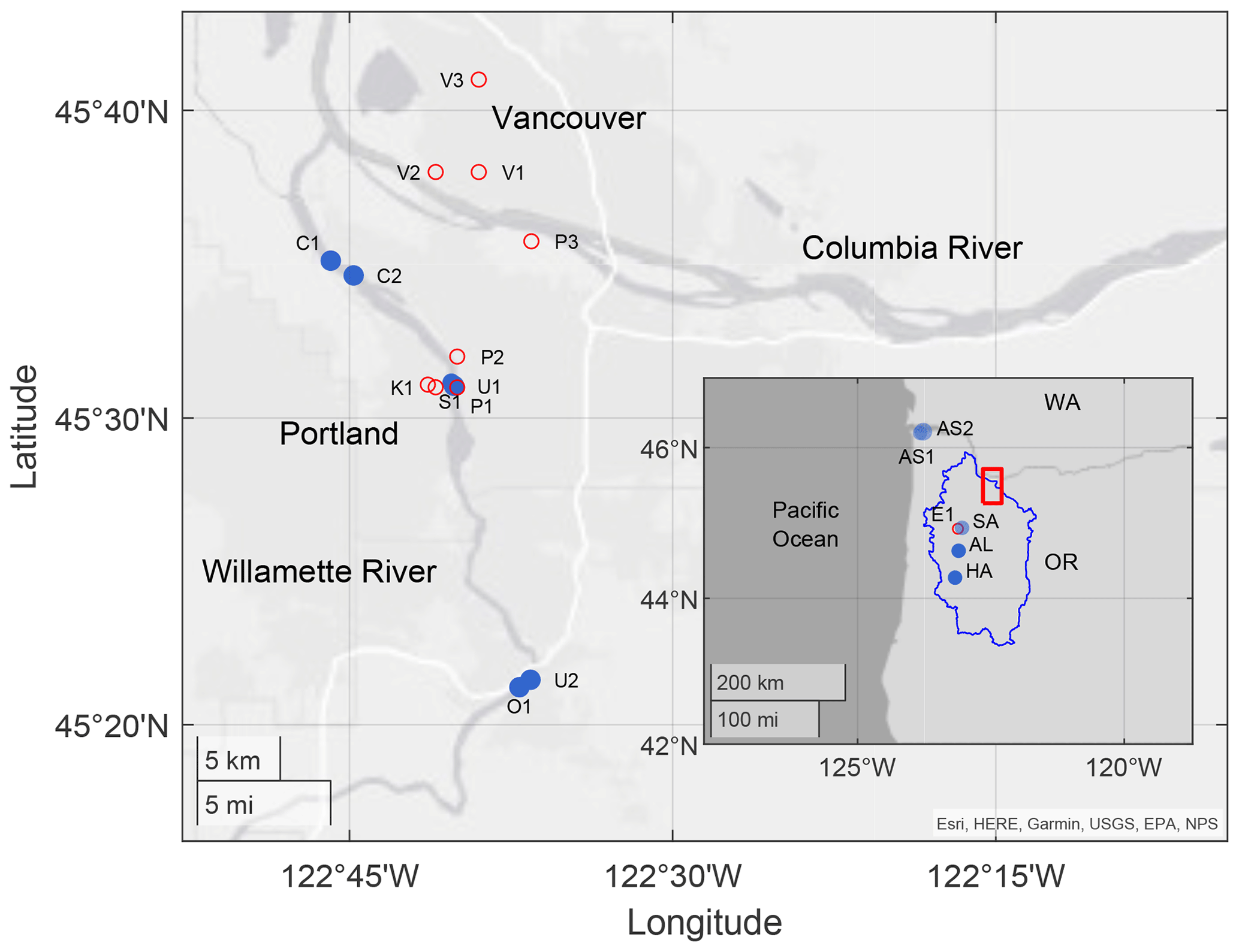
Figure 1Site map with locations of Tw (blue, closed circles) and Ta (red, open circles) measurements. The red bounding box in the inset denotes the Portland–Vancouver metropolitan area depicted in the larger figure. The Willamette River watershed boundaries are denoted in blue. OR is Oregon, and WA is Washington. Abbreviations and period of record of the measurements are provided in Table 1.
2.1 Study area
The Willamette River (Fig. 1) has a 1971–2020 mean annual discharge of 940 m3 s−1 and drains 29 700 km2 of coastal Oregon (Fig. 1; Branscomb et al., 2002). It is the 13th largest river in the contiguous United States by volume (Wallick et al., 2022), and its waters discharge into the larger Columbia River 162 km from the Pacific Ocean. The lower Willamette River, the focus of this study (Fig. 1), is 43 km long. It is influenced by ocean tides most of the year and by backwater from the Columbia River, particularly during spring (Helaire et al., 2019). Because of its location near the mouth, the lower Willamette is influenced by, and integrates climate changes and local anthropogenic changes within, its entire basin.
Evaluating changes in Tw in the lower Willamette River is important because it influences the long-term viability of salmon and other vulnerable and endangered species (Mantua et al., 2010; Bottom et al., 2011, Isaak et al., 2012; Caldwell et al., 2013; Clemens, 2022). Above a threshold of 18–21 ∘C, various species of salmon, steelhead, and trout are stressed and become more susceptible to disease (OR-DEQ, 2006; Mantua et al., 2010). The migration and spawning of Willamette River fish such as Pacific lamprey (Entosphenus tridentatus) (Clemens et al., 2016) and Chinook, coho, and chum salmon (Richter and Kolmes, 2005) are directly impacted by elevated temperatures. Because of such ecological effects, regulations require that the 7 d average of the daily maximum temperature should not exceed 20 ∘C, with a lower threshold set for rearing and spawning streams (e.g., OR-DEQ, 2006).
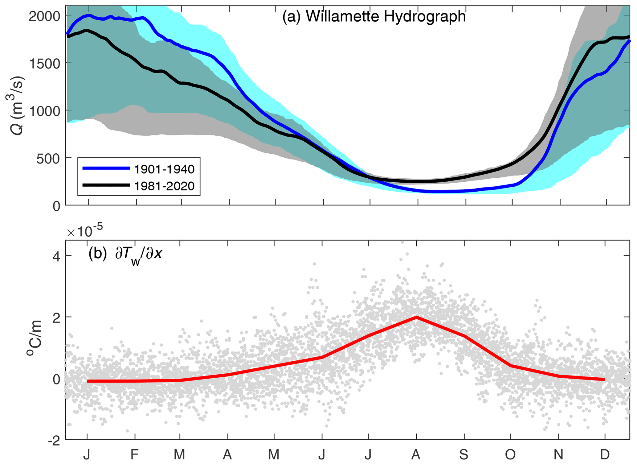
Figure 2(a) The Willamette hydrograph at Portland, Oregon, for the pre-reservoir (1901–1940) and modern (1981–2020) periods, and (b) the horizontal Tw gradient between Albany, Oregon, and Portland, Oregon, for the 2000–2017 time period, in units of 10−5 ∘C m−1. Positive indicates that downstream measurements in Portland are warmer. Shading in (a) denotes the 25th and 75th percentile of measured discharge. The along-river distance between Portland and Albany is 169 km. The red line in (b) denotes the monthly average. Tick marks denote the middle of each month.
The Willamette Basin has a temperate climate marked by overcast conditions from October–May and predominately dry conditions from June to September. Average annual precipitation on the valley floor is 1–1.3 m yr−1, with up to 5 m occurring in mountainous headwater areas (Baker et al., 2002). Rainfall and high-discharge events occur primarily between November and March (Fig. 2a). Historically, snowmelt contributed to elevated flows in the March–May time frame (Fig. 2a), but a combination of declining snowpack and flow regulation has reduced spring discharge (Mote et al., 2018; Rounds, 2010). During summer, 60 %–80 % of river water derives from high-elevation regions above 1200 m, either as direct snowmelt or as groundwater (Brooks et al., 2012). Late-summer discharge has increased, however, because of the managed release of water.
The mainstem Willamette River, which runs 300 km south to north, has been extensively modified since the latter part of the 19th century, first for navigation and agriculture and later for flood control. Land under irrigation was minor before 1910 but increased 8-fold from 13 500 to 110 000 ha between 1945 and 1979 (Sedell and Froggatt, 1984). Before European settlement, the floodplain was maintained in a prairie or savannah-like condition by burning (Christy and Alverson, 2011). After burning ceased (late 1700s), the 3–7 km wide floodplain became covered by a dense riparian forest and had two to five shallow, braided channels (1.5–3 m depth) that evolved each year (Thilenius, 1968; Sedell and Froggatt, 1984; Gregory et al., 2002a; Wallick et al., 2022). Beginning in the 1870s, but particularly in the first half of the 20th century, the river was reduced to a primarily single-thread stream and shortened by nearly 20 km (Sedell and Froggatt, 1984; Gregory et al., 2002a). Shading was much reduced (Lee, 1995; OR-DEQ, 2006). Bank-stabilization measures began in the late 1800s and occurred most prominently during the 1930s–1960s; approximately 25 % of Willamette River banks now have engineered protection (Gregory et al., 2002b). Further, from 1870–1950, approximately 65 000 dead trees (up to 60 m long with a diameter of 0.5–2 m) were removed (> 500 km−1; Sedell and Froggatt, 1984). As a result of these efforts, off-channel alcoves and sloughs – often 2–7 ∘C cooler than the mainstem – decreased in extent by 70 %–80 % (Landers et al., 2002). Additionally, forested floodplain decreased by 75 %–90 % (Landers et al., 2002; Gregory et al., 2019). Dredging further altered the river upstream of ∼ river kilometer (Rkm) 50, particularly before 1930 (Willingham, 1983); much more extensive dredging has occurred in Portland Harbor (e.g., Helaire et al., 2019). The depth of the river is currently ∼ 12 m in the lower ∼ 20 km of the Willamette, the focus area of our study (Fig. 1). Depths gradually reduce to a centerline depth as shallow as 1.5–2 m around Rkm 280 (US Geological Survey (USGS), 2003).
A total of 371 reservoirs and impoundments have been built in the Willamette Basin, with a combined capacity of more than 3.3 km3 (Payne, 2002). Given a mean discharge of about 980 m3 s−1 (Naik and Jay, 2011), these reservoirs potentially store ∼ 10.6 % of the annual average flow. The majority were built between 1950–1980, with only 23 built pre-1950 and about 25 after 1980 (Payne, 2002). A total of 11 federal storage and flood control reservoirs were built between 1953 and 1969 with a combined maximum storage capacity of 2.57 km3 (Payne, 2002; Rounds, 2010). The two federal reservoirs built in the 1940s were relatively small (combined capacity of 0.18 km3); therefore, we consider the period before 1953 to be pre-river flow regulation. Hydrological records suggest that flood control exerted some influence in the 1954–1969 period, reducing peak flows during the December 1964 flood considerably; thus, the modern hydrological regime began during this period (Waananen et al., 1970; Gregory et al., 2002c).
Reservoirs have increased the surface area of water within the system by about 200 km2, with the majority (80 %–85 %) occurring in the 13 federally operated water projects (Payne, 2002). An additional net increase of ∼ 50 km2 in water surface area is estimated for the Willamette Valley since 1851 (Gregory et al., 2002d), in part from water impoundments. By comparison, channelization between 1850 and 1995 removed ∼ 17 km2 of water surface on the mainstem Willamette, from 76 to 59 km2 (Gregory, 2002a). Summertime peak Tw values at reservoir sites are hypothesized to have decreased after dam construction; at the same time, fall Tw has increased (e.g., Angilletta et al., 2008; Rounds, 2010).
Table 1In situ Tw measurements used to obtain a composite record of daily minimum in Portland, 1881–2021. Locations ordered based on start date and originating agency. Precision based on measurement significant figures. A bias correction was applied to standardize measurements to the daily minimum Tw, based on the time of day of the measurement, and to account for the Tw gradient between Portland and upstream stations. River kilometers (km) from the mouth are indicated for the Columbia River (CR) and the Willamette River (WR). Additional information on the data used in the composite in situ Tw series is included in the data repository.
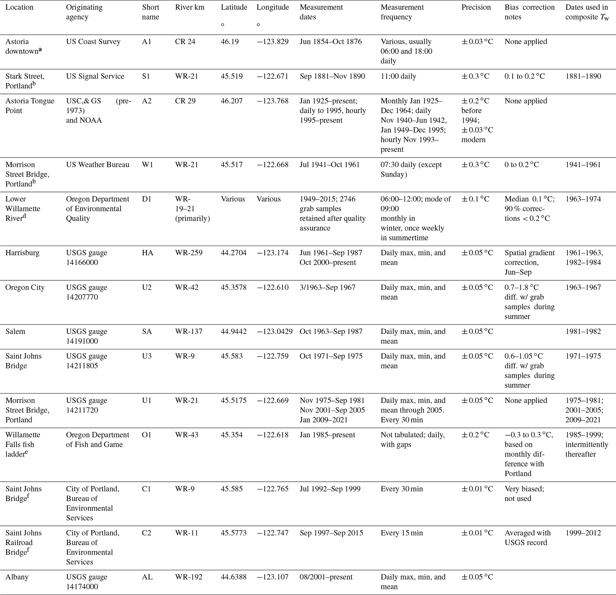
Stations ordered by start date, with earliest measurements first. All times given in local standard time. Bias corrections are subtracted from raw measurements on a monthly basis to obtain daily minimum; a positive value indicates a downward adjustment. Coordinates provided in the North American Datum of 1983. The locations for the measurements at Stark Street, Astoria downtown, Willamette fish ladder, and the City of Portland are estimated based on available data. River kilometers measure the thalweg distance from the mouth of the Willamette, except for Astoria which is on the Columbia River. a Measurements obtained from US National Archives; see Talke et al. (2020). b Measurements obtained from National Centers for Environmental Information. c Data obtained from NOAA; grab samples from 1925–1995, approximately daily, generally between 10:00–13:00; median ∼ 11:30. d Data obtained from US EPA STORET database. Measurements often made from bridges in the Portland metropolitan area, including the Hawthorne Bridge, the Steel Bridge, and the Burlington Northern Railway Bridge. Samples pre-1960 discarded because of lack of time stamp. Grab samples after 12:00 not considered to avoid afternoon heating signal. Pre-12:00 data adjusted to daily minimum on monthly basis based on modern USGS data. Measurements at 1–3 d frequency in 1964–1972. e Data from 1985–1999 obtained directly from agency; post-1999 records available online. Based on a comparison using 2001–2004 data, an average warming of 0.2 to 0.3 ∘C occurs between Willamette Falls and Portland from July to September. A cooling of up to 0.3 ∘C occurs between March and May. Little variation occurs at other times. f Obtained directly from agency; pre-2000 data also obtained from Berger et al. (2004).
Table 2Meteorological stations used to develop statistical models and associated root mean square error (RMSE) of Tw obtained for different calibration periods (annual, summer, and winter). The RMSE represents either the daily or monthly averaged difference with in situ Tw measurements, in degrees Celsius. Station identification (ID) numbers are from the US National Weather Service. Measurement dates denote the time period in which daily maximum temperature was recorded at the given location. The latitude–longitude values for Eola (near Salem, Oregon) are estimated. All stations except Vancouver are in Oregon.
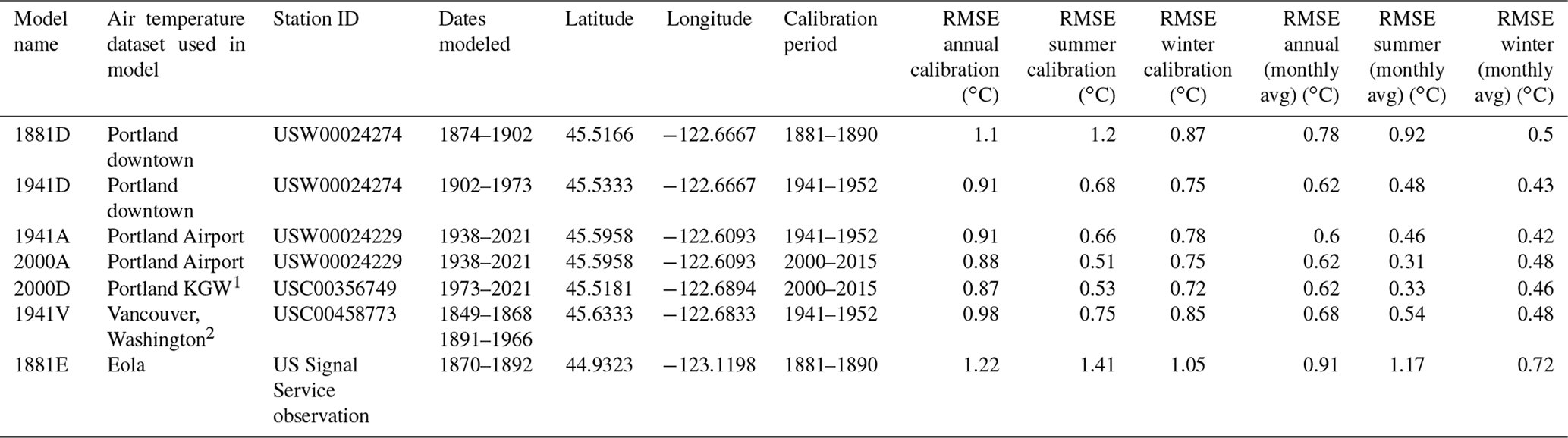
1 The annual RMSE between measurements and the climatological average is 1.86, 1.46, and 1.43 ∘C for the 1881–1890, 1941–1952, and 2000–2015 calibration periods, respectively. 2 The 1973–1999 measurement was at a slightly different location of (45.517∘ N, −122.683∘ E). The elevation of the 1973–present dataset is ∼ 48.5 m. The lapse rate for the standard atmosphere (6.5 ∘C per 1000 m) suggests that the difference to a measurement at sea level is ∼ 0.3 ∘C. An observed difference in average daily maximum temperature at Portland Airport (17.46 ∘C, < 10 m relative to sea level) and Portland KGW (17.07 ∘C) between 2000–2020 is therefore mostly caused by elevation differences. 3 The Dec. 1849–1868 measurement at Fort Vancouver was made by the US Signal Service; the approximate location was 45.633∘ N, −122.65∘ E and was several kilometers east of the 1891–1966 measurement. The gauge was moved in 1966 to a higher-elevation location with a known bias (Mote et al., 2003). The 1966–present data are therefore not used.
2.2 In situ measurements
Measurements were obtained from multiple federal, state, and local archives and databases to assess meteorological and fluvial conditions between 1850–2021 (Fig. 1; Tables 1 and 2). We found and digitized previously unused records from the US Signal Service (1881–1890) and the US Weather Bureau (USWB) (1941–1961) held at the National Centers for Environmental Information (NCEI). A spot check of US Army Corps of Engineers records from Willamette Rkm 10.5 from 1941–1942 (Moore, 1968) showed a general consistency with individual USWB measurements, to within 1 ∘C. Modern records of Tw have been available from the US Geological Survey (USGS) since 1961, with ∼ 26 station years available in the Portland metropolitan area since 1971 (Table 1). These federal records are supplemented by additional state and local records. Intermittent grab-sample measurements of Tw are available from the Oregon Department of Water Quality, particularly during summer (1949, 1953–present; obtained from the City of Portland). Additionally, nearly continuous daily measurements of Tw at the Willamette Falls fish ladder from 1985–2020 were obtained from the Oregon Department of Fish and Wildlife. Finally, continuous records were obtained for 1992–1999 and 1997–2015 at two locations near Portland (City of Portland; see also Annear et al., 2003).
We combined the above Tw records to obtain a 90-year record of in situ Tw covering 64 % of the 1881 to 2021 period (Table 1). Daily measurements were adjusted to the daily minimum temperature because most historical measurements were made in the morning. The adjustment, typically ∼ 0.1 ∘C, was based on the monthly averaged differences between measurement time stamps and the daily minimum in modern, high resolution data (Table 1). The composite 1881–2021 record uses lower Willamette records when available and the nearest mainstem data otherwise (if available). Records in Oregon City and farther upstream were adjusted for spatial heating effects through the use of monthly averaged gradients observed between coterminous measurements from 2000–2017. Most adjustments for spatial variability were minor (< 0.3 ∘C), except for 1962 and 1983–1984, for which the only available measurements were from the middle or upper Willamette River. Additional notes are included in Table 1, and the sources of data in the composite are included in the data record (see data repository).
Additionally, we use Tw measurements from the lower Columbia River to check our model estimates (see Sect. 2.4) during periods with no other data (Fig. 1, Table 1). Tw was measured up to twice daily at Astoria, approximately 24 km from the ocean, from 1854–1876 (Talke et al., 2020). Monthly estimates of Tw at Tongue Point (Rkm 29) are available from 1925–1964 (U.S. Coast and Geodetic Survey (USC & GS, 1967), and daily records were obtained from 1940–1942 (Moore, 1968) and 1949–present from the National Oceanographic and Atmospheric Administration. Before 1950, surface waters at Astoria were generally freshwater or brackish during typical flow conditions (Al-Bahadily, 2020; USC & GS, 1967) and therefore are representative of river Tw values.
The availability and quality of in situ data informs our choice of model calibration periods and interpretation of model/data comparisons. Monthly averages of the USGS, DEQ (Oregon Department of Environmental Quality), and City of Portland data from 2009 to 2015 agree to within 0.1–0.2 ∘C, indicating that modern measurements from the last 2 decades are consistent and of high quality. This comparison also shows that grab samples from the water surface compare favorably with other methods. Measurements by the US Signal Service (USSS) (1881–1890) and USWB (1941–1961) were made at a first-order weather station by trained professionals and appear to be of high quality (see, e.g., MWR, 1881–1890); however, little independent verification is possible. Evaluation of data from 1962 to the mid-1990s indicates some periods with lesser quality in which different measurements disagree with each other. For example, summertime measurements from a thermograph in Oregon City (1963–1967) are as much as 1.8 ∘C higher (monthly average) than coterminous grab samples; a smaller difference occurs between Saint Johns Bridge measurements (1971–1975) and grab samples (Table 1). Because the typical difference between such measurements is reported to be < 1 ∘F (0.56 ∘C) (Moore, 1967), an undocumented instrumental or measurement issue occurred.
Meteorological and flow records
A nearly complete USGS discharge record for the lower Willamette River is available from 1893 to present, with intermittent values available from 1878–1892. Daily discharge is available from the USGS in Portland from 1972 to present (USGS gauge 14211720). Routed estimates of discharge at Portland are available for earlier periods from 1878 forward from Jay and Naik (2011), based on USGS measurements at Albany (USGS gauge 14174000) and Salem (USGS gauge 14191000).
Several sources provide records of daily maximum Ta in the Portland–Vancouver area (Table 2). Daily USSS weather records at Vancouver (1849–1868) and Eola (1870–1892) were provided in digital form by the Midwestern Regional Climate Center (https://mrcc.purdue.edu/, last access: May 2023). Additional daily records from the USWB and the National Weather Service from Portland and Vancouver cover the 1874–present period and were obtained from NCEI.
Air temperature (Ta) records were carefully evaluated for potential bias and consistency with each other (Table 2; see Fig. 1 for locations). For example, the Vancouver record from 1895–1965 averages 0.4 to 0.5 ∘C warmer than the downtown Portland record. Average Portland Airport values were < 0.05 ∘C cooler than the downtown Portland Weather Bureau readings between 1940 and 1948. Thereafter, the downtown Portland record warmed more quickly and was 0.54 ∘C warmer than the airport from 1960–1969. The modern temperature record at the KGW television station in Portland (1973–present), located at 48.5 m above sea level, is slightly cooler from 1991 to 2020 (annually averaged daily maximum of 17.08 ∘C) than that at Portland Airport (17.47 ∘C). Under standard atmospheric conditions, with a lapse rate 6.5 ∘C per 1000 m, a difference of ∼ 0.3 ∘C is expected between these records as compared to the actual difference of 0.39 ∘C. Thus, we conclude that the measured difference between the stations is almost entirely explainable by elevation effects. After adjusting for mean biases, the root mean square error (RMSE) between the various daily Portland Ta records is about 1–1.1 ∘C from 1940–present. The RMSE between Vancouver and Portland Ta is larger (1.5–1.6 ∘C), possibly because of small differences in local climate. The influence of these small differences on our Tw model results is explored later.
2.3 Advection–diffusion equation
To develop our statistical model approach, understand its limitations, and motivate its form, we first consider the underlying physical dynamics. Heating and cooling of river water is governed by the advection–diffusion equation (ADE; e.g., Fischer et al., 1979). When vertical and cross-sectional variations in Tw are neglected, the 1-D ADE for Tw as a function of time t and along-channel coordinate x (positive downstream) reads
where K is a horizontal diffusion coefficient, u is river velocity, H is the sum of heat flux into or out of the system, d is the cross-sectionally averaged depth, ρ is the density of water, and cp is the heat capacity of water. This simple ADE does not consider groundwater flow, which cools the off-channel alcoves of the Willamette River during summer (Faulkner et al., 2020).
We use scaling of Eq. (1) to determine the relative importance of the advection, diffusion, and heating terms, relative to the time rate of change . An evaluation of measurements suggests that the diffusive term is negligible but that the nonlinear advective term is likely influential during summer, due to a positive (Fig. 2). Nonetheless, the low velocities in late summer counteract the influence of large . Based on our scaling, the heating term is usually the leading-order term that drives the time rate of change of Tw, (see also Wagner et al., 2011). When advection and diffusion are unimportant, the nonlinear heating term () drives the term. The term can be linearized, enabling use of a linear regression approach in which Tw is a function of Ta and river discharge Q (see Mohseni and Stefan (1999) or the Supplement for a more detailed discussion of linearization assumptions). The river discharge term incorporates the net influence of precipitation, snowmelt, and groundwater recharge.
The discussion above suggests that linear regression models have a basis in the underlying physical dynamics. However, a number of assumptions and approximations must be made to convert Eq. (1) to linear form, and a linearized representation of average conditions during a particular season may work less well under unusual or extreme conditions. Simplifying heating to a linear function of Ta and Q works best during periods of relatively constant Tw and river discharge (see Mohseni and Stefan, 1999). In summary, in Eq. (1) can be linearized and expressed in terms of three basis functions, Tw, Ta, and Q (see Supplement for more information):
where bw, ba, and cQ are coefficients, and the minus sign indicates that river flow reduces Tw. Using the approximation , we find that Tw at time step n is equal to the Tw at the previous time step (n−1) plus a correction that is a function of Ta and Q:
Equations (2) and (3) depict an autoregressive (AR1) process. Hence, at time n−1, Tw is a function of the Tw at time n−2, and the Tw at n−2 depends on Tw at n−3. Equation (3) can be rearranged such that is on the left-hand side only. If we develop and then substitute similar solutions for , , … into this modified version of Eq. (3) and solve for , we find that at time t,
where aτ and bτ are regression coefficients at time lag τ, C is a constant of regression, and the time period j is chosen to be long enough that the coefficients aτ and bτ at large time lags effectively become negligible and/or statistically insignificant. Further, at the large time lag τ=j, the influence of the time-lagged water temperature term in Eq. (3) becomes negligible and drops out. Note that the negative sign in Eq. (3) has been subsumed into coefficient bτ. The coefficients aτ and bτ can be modeled using an exponential filter approach (e.g., Al-Murib et al., 2019); here, as explained below, we estimate the coefficients directly.
2.4 Statistical model
We model Willamette River Tw by applying a stochastic modeling approach to Eq. (4) (see, e.g., Benyahya et al., 2007). In this approach, the dependent variable (Tw) and the independent variables (TA and river discharge Q) are decomposed into a long-term climatological average and a time-varying component. The deviation from climatology is modeled, and the result is added back to climatology to obtain estimates of Tw. A similar approach has also been applied to the Columbia River (Scott, 2020; Scott et al., 2023); other statistical models applied to this region include Moore (1967), Donato (2002), Bottom et al. (2011), and Mayer (2012). For a generic variable X(t) measured daily, we define the climatological average as
where T = 30 d, t is the integer number of days since the start of the year, y1 is the beginning year of the time series (e.g., 1881), y2 is the end year (e.g., 1890), and the overbar represents the climatological average. The 95 % uncertainty in the climatological average is given by , where t∗ = 1.96 for a large sample size N, and σ is the standard deviation. In practice, the number of years we used to define the climatological average is limited by available data.
The deviation from climatology, caused for example by a heat wave, is defined as
For a model to have predictive and explanatory power, it must exhibit a root mean square error (RMSE) with in situ data less than that of X′(t). Substituting Eqs. (5) and (6) into Eq. (4), and considering only deviations from climatology, our basis function becomes
where the prime indicates a deviation from climatology, and other terms are as defined in Eq. (4). Based on experimentation, we use daily lags up to 2 weeks. Thereafter, we use average to obtain a statistically significant correlation. A 15 d average is used for day 15–30, and 30 d averages are used thereafter, up to 6 months. Similarly, river discharge Q′ is averaged using a 10 d average for day 1–10, a 20 d average for day 11–30, and a 30 d average thereafter.
A total of seven statistical models are developed from Eq. (7), using data from the 19th century (1881–1890), mid-20th century (1941–1952), and modern period (2000–2015) (see Table 2). The models differ in the location of air temperature data and time period used. The three calibration periods were chosen based on available data; they approximate (nearly) pre-development conditions, pre-flood control conditions, and modern conditions. The models are named based on the first year of calibration data and the first letter of the meteorological station used; for example, 1941V and 1941D are models trained with 1941–1952 data from Vancouver and downtown Portland, respectively (Table 2). Within each model, we further developed a summer sub-model (July–September), a winter sub-model (January–March), and an annual model, based on all available data. Experimentation was used to obtain the optimal time span of winter and summer models, and the annual model is used for months not covered by the winter or summer models. For example, the summer model covers July to September, consistent with the observation that the horizontal temperature gradient is largest during this period (Fig. 2b). Through experimentation, we also determined that discharge only produces a statistically significant effect for summertime models based on 1941–1952 and 2000–2015 data (i.e., not winter or annual models).
Each statistical model produces an estimate of Tw over the period of record of its underlying Ta record (Table 2; data available in the Supplement). Based on output time series, a composite estimate of modeled Tw was produced using the best available statistical model. A compromise was required when deciding which era of model to use in the composite because there is no absolute delineation between pre- and post-reservoir conditions or between a nearly natural and substantially altered landscape. Models based on Vancouver Ta measurements were used pre-1868, Eola Ta measurements from 1870–1874, downtown Portland data from 1874–1939, and Portland Airport data thereafter. For each year, the two seasonal sub-models were used, with the annual sub-model used at other times. The mid-20th century calibration, representing pre-reservoir, post-landscape change conditions, was applied to the 1900–1960 period (1941A model); thereafter, we assume modern flood control, and applied the modern calibration (2000A model). Estimates from 1869–1899 used the calibration based on 1880s Tw data (1881D model). No overlap occurred between Vancouver Ta and Willamette Tw measurements during the 19th century. Hence, pre-1868 estimates used the mid-20th century calibration to Vancouver Ta (the 1941V model), since a 19th century calibration was unavailable.
The skill of each statistical model was assessed by evaluating the root mean square error (RMSE) between the composite model estimate and measurements. Our values are compared against the RMSE found between measurements and climatology. The uncertainty of modeled temperature estimates was assessed using a Monte Carlo approach. A total of 2000 possible ensembles of the model coefficients were created, under the assumption that coefficient uncertainty (obtained by the linear regression) was normally distributed. The 95th percentile of the resulting spread of solutions is reported.
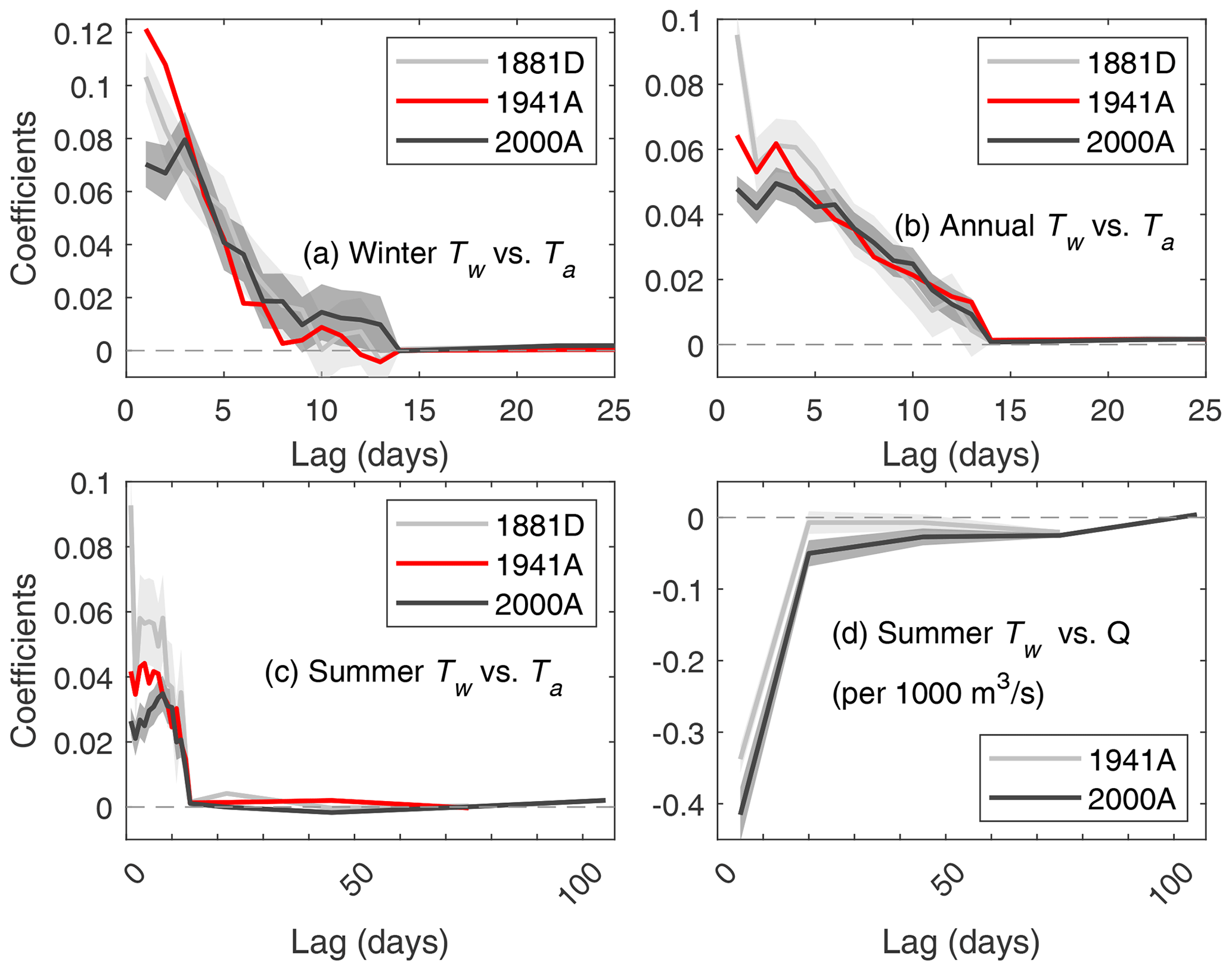
Figure 3Coefficients for statistical model vs. time lag for (a) Ta in the winter model (November–March), (b) Ta in the annual model (all months), (c) Ta in the summer model (July–September), and (d) discharge Q in the summer model (July–September). The 1881 model is calibrated to 1881–1890 Tw data, the 1941 model is calibrated to 1941–1952 Tw data, and the 2000 model is calibrated to 2000–2015 Tw data. The letter denotes whether Ta data were sourced from downtown Portland (D) or from the airport (A). Similar results are found for the model based on Vancouver Ta data (not shown). No statistically significant effect of river discharge was found for winter or annual models and the 1880s summer model. These results are not shown.
2.5 Attribution analysis
We approximate the influence of changing air temperatures, changing river discharge, and the integrated effect of river system changes through experimentation using our statistical models. The following first-order effects are approximated:
-
Climate change impacts. Climate change has driven changes in the 30-year average climatology of daily air temperature in the region (e.g., Mote et al., 2019). We estimate the influence of changed air temperature climatology by running our modern statistical model (model 2000A; see Table 2) using historical downtown climatology (1875–1904) and modern Portland Airport climatology (1991–2020) (daily timescale). River flow is kept constant and does not influence results. The difference between these scenarios is attributed to climate change. The uncertainty in modeled Tw is assessed by perturbing input climatology with plausible uncertainty and bias estimates in Ta.
-
Effect of altered river flow. Changes in river flow seasonality, caused primarily by water resources management but also influenced by changing snowpack (e.g., Naik and Jay, 2011), can influence water temperatures in our 1941 and 2000 era summer models (Table 2; river flow was not statistically significant in 1881 era models). The change in the river hydrograph (see Fig. 2a) is applied to the 1941 and 2000 era models (Table 2), with the Ta input kept the same between models. The difference in model output shows the influence of altered average river flow on modeled Tw for the July–September time frame between pre-reservoir (1901–1940) and modern (1981–2020) conditions.
-
Integrated system changes. Over the past 150 years, multiple landscape and watershed changes, including loss of riparian habitat and reservoir construction, have occurred (Sect. 2.1). We investigate their net influence on Tw by applying the same river flow and Ta data from 2000–2020 to models from different eras (Table 2). Because the input into each statistical model is identical, any differences in output Tw are caused by changes in model coefficients (Eq. 7). The uncertainty analysis in Sect. 2.4 is applied to determine whether differences are statistically significant, consistent with the hypothesis that river system changes have altered the river's response to external heating and other forcing.
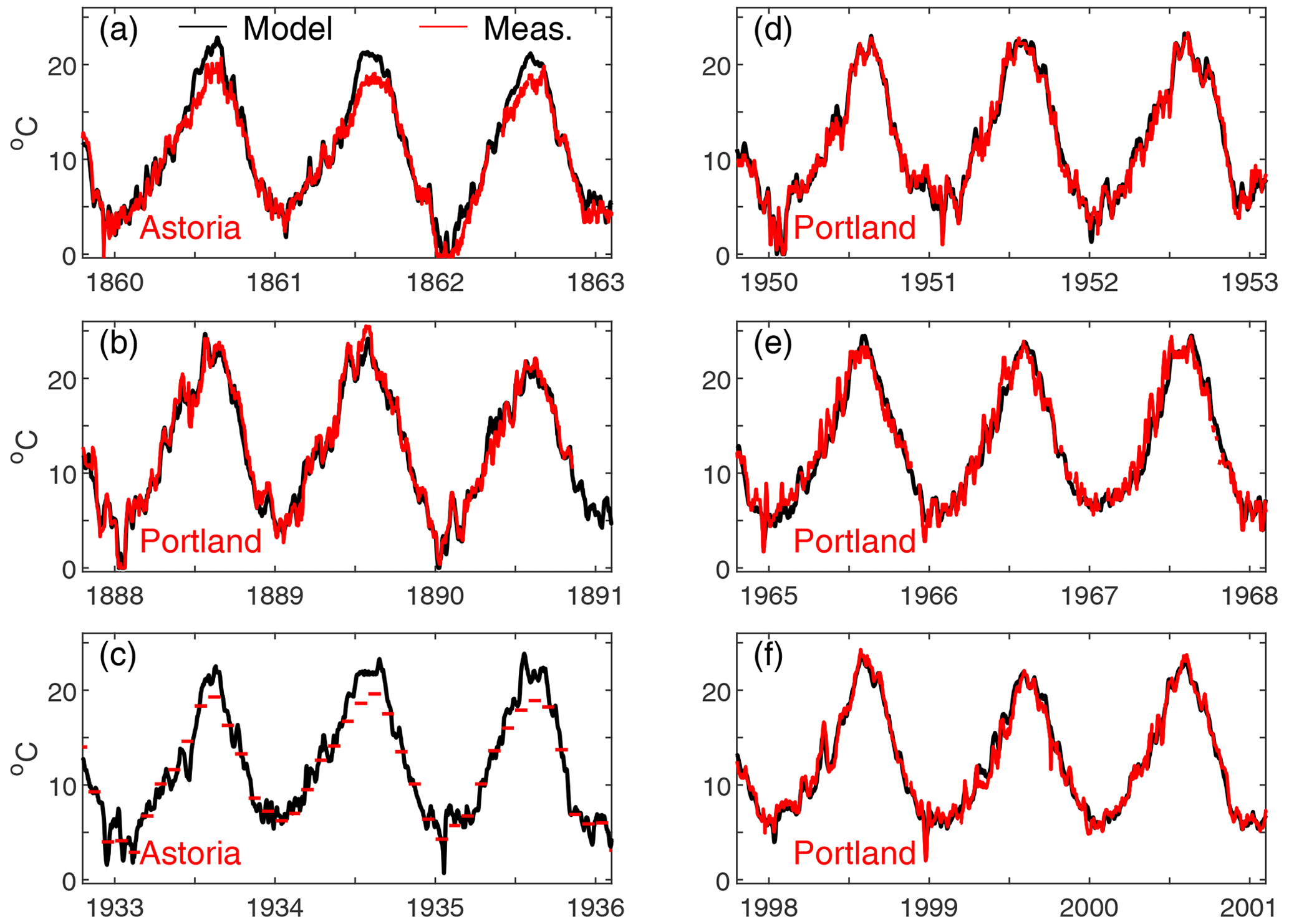
Figure 4Comparison of modeled and measured Tw for six 3-year periods. The composite Portland Tw is used in (b), (d), (e), and (f), while Astoria measurements are used in (a) and (c). Only monthly averages of Tw are available at Astoria from 1925 to 1940 and 1943–1948 (see Table 1). Black is modeled, and red is measured.
3.1 Model assessment
Results show that the model coefficients (see Eq. 7) generally decrease in magnitude as Ta (Fig. 3a–c) and river discharge (Fig. 3d) are lagged backwards in time. Further, the decorrelation structure is different for the 19th, mid-20th, and 21st century models (Fig. 3); hence, for the same forcing, these statistical models will produce a different output (Eq. 7). Statistically significant coefficients are found at up to a 3-month lag in the 1880s model and 4 months in the others. The magnitudes of coefficients at 2–4-month lags are larger today, at ∼ 0.0025 per day (modern) vs. ∼ 0.0017 per day (1940s; annual model). As discussed later, the changes in the statistical model between eras likely occur due to the integrated effect of land-use and water management changes.
Time-series comparisons of modeled and observed Tw (Fig. 4) and statistical evaluations (Table 2) confirm that the stochastic model reproduces year-to-year differences in Tw and weekly–monthly perturbations caused by persistent warm/cold weather. Some synoptic-scale events of less than a week are only partially captured, possibly because of factors not included in the model, e.g., cloud cover, wind, or depth changes due to backwater from the Columbia River (see also Wagner et al., 2011) and the tendency of statistical models to underestimate extremes. The RMSE between the measured and modeled daily minimum Tw varies from 0.87 to 1.1 ∘C for the annual model, with an RMSE as low as 0.53 and 0.72 ∘C for the summertime and wintertime models, respectively (Table 2). Results are less good using Eola (1870–1892), a historical weather station which was located ∼ 70 km from Portland and may imperfectly represent local meteorological forcing. For monthly averaged estimates, the RMSE varies from ∼ 0.3 to 0.9 ∘C, with the best agreement obtained during the modern period and the summertime sub-models (Table 2).
Our statistical model results compare favorably with numerical models, other statistical approaches, and climatology. For example, the RMSE at Portland for a calibrated numerical model based on measurements from April–September 2002 was 0.43 ∘C (Berger et al., 2004), compared to 0.52 ∘C for our model over the same period. Similarly, our models perform significantly better than estimates based on Tw climatology, which have a root mean square error (RMSE) of 1.86, 1.46, and 1.43 ∘C for the 1881–1890, 1941–1952, and 2000–2015 calibration periods, respectively (see Table 2). Our results compare well with traditional linear regression and stochastic models, which typically report a RMSE of ∼ 0.6–1.9 ∘C, depending on model type, river size and location, and averaging period (e.g., Caissie et al., 1998; see also review by Benyahya et al., 2007, and references therein). More recent statistical models, including air2stream (Toffolon and Piccolroaz, 2015) and machine learning approaches (e.g., Feigl et al., 2021), report an RMSE of 0.5–1 ∘C on a daily scale, similar to the results presented here (Table 2). Results are also comparable to numerical models that generally have an RMSE < 1 ∘C (e.g., Dugdale et al., 2017). We conclude that our statistical models accurately represent the most important factors affecting Tw, as long as the underlying measurements driving the model are reasonably accurate and representative of local conditions.
Modeled Tw estimates based on models using different Ta data series (Table 2) compare well with each other, with similar averages and variability. During their period of overlap from 1940–1973, daily modeled Tw values are slightly larger (0.08 ∘C) using the airport model (1941A) than the downtown Portland model (1941D). Similarly, the Vancouver model (1941V model) is 0.02 ∘C lower than the airport model (1941A) between 1940 and 1965. For the same periods, the daily RMSE between the 1941A model Tw and the 1941D and 1941V models is 0.29 and 0.32 ∘C, respectively. For the 1896–1965 period, the 1941D and 1941V models show a mean difference of 0.06 ∘C (Vancouver larger) and an RMSE of 0.37 ∘C. These observations provide an order-of-magnitude estimate of the aggregate influence of input data and model variability on uncertainty, whether caused by spatial variations in Ta, differences in the statistical coefficients, or instrumental measurement precision and bias errors. The consistency and small RMSE between model results improve our confidence in both the input data and the results.
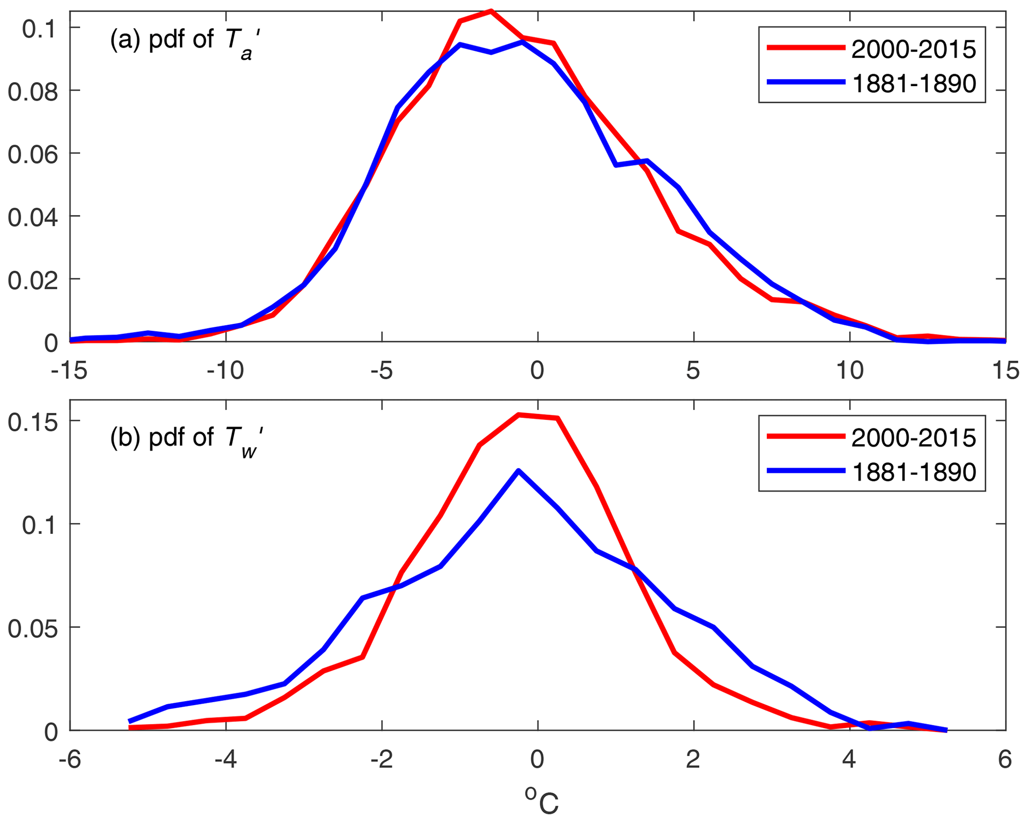
One of the factors driving the larger RMSE in the historical model is the larger overall system variance measured for 19th century Tw. The typical distribution of Ta anomalies from the climatological mean has remained stationary between different time periods, and the standard deviation is nearly the same (within ∼ 5 %; Fig. 5). However, between the 1880s and the 2000–2015 period used for calibration, the distribution of measured Tw anomalies markedly contracted, and the standard deviation decreased from 1.86 to 1.42 ∘C (Fig. 5). Since the distribution of Ta anomalies remained similar, a likely explanation for the decreased variance in Tw is anthropogenic change to the local environment (e.g., flow regulation, landscape changes, channel deepening), namely alteration of the riverscape (Peipoch et al., 2015) (see Discussion).
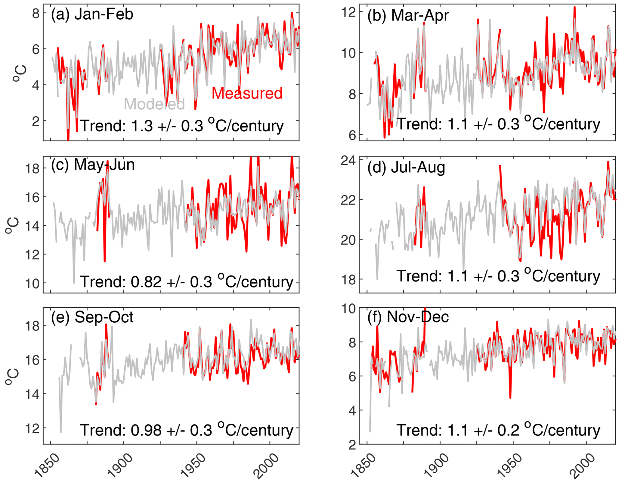
Figure 6Seasonal trends in water level, averaged over 2-month water periods. Measurements (red) and model results (grey) are correlated. The trends and 95 % confidence interval are based on a linear regression to model results, 1850–2020; November–April data for 1854–1876 are from Astoria (see Talke et al., 2020). Note different y-axis scales.
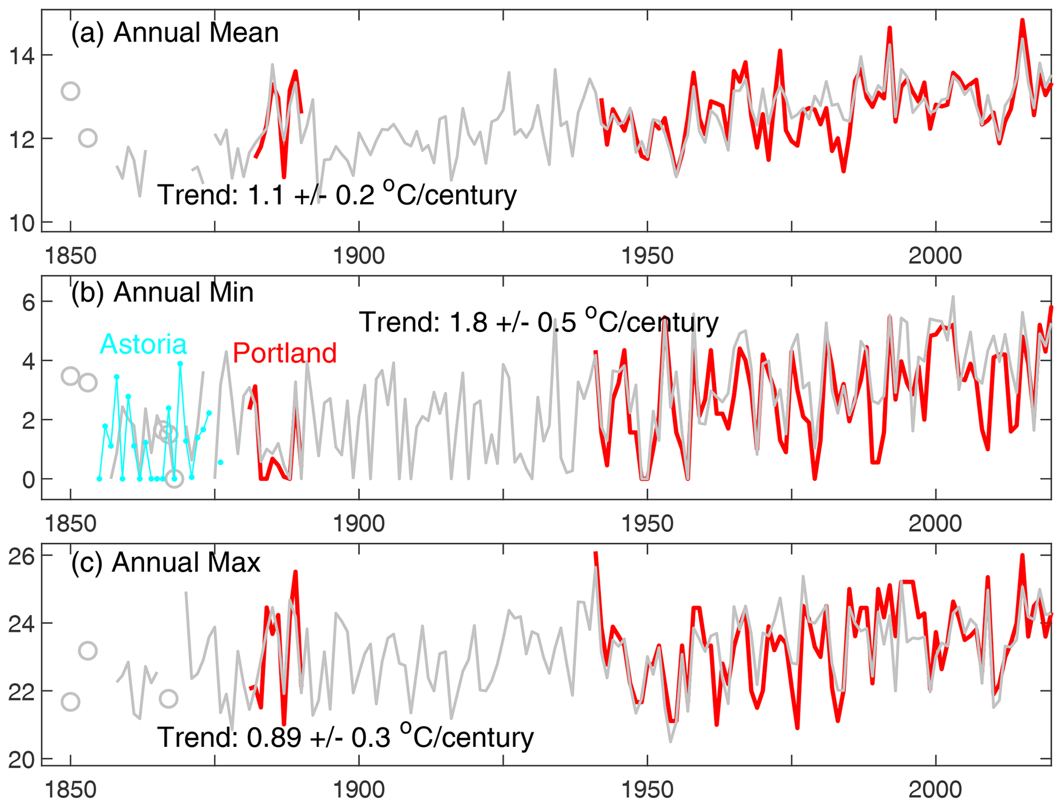
Figure 7Time rate of change of annual mean, annual minimum, and annual maximum Tw. Grey denotes model data, red denotes data from Portland region, and cyan denotes Tw measurements in Astoria (annual minimum only, b). The trend is calculated by results of the regression fit to the model over the 1850–2020 period. Evaluation is based on daily minimum Tw (see Sect. 2). Years in the 1850s and 1860s without sufficient model data are excluded.
3.2 Water temperature changes in lower Willamette
Measurements and model results show that water temperatures have increased steadily since the 1800s. Increases are observed at all times of the year (Fig. 6), leading to an increase in annually averaged Tw of 1.1 ± 0.2 ∘C per century (Fig. 7). The largest increase occurred in winter; during January–February, the trend in average Tw is 1.3 ± 0.3 ∘C per century (Fig. 6a). Similarly, the minimum annual water temperature is increasing quickly, at 1.8 ± 0.5 ∘C per century (Fig. 7b). The smallest bimonthly averaged trends occur in late spring, during May–June (0.82 ± 0.3 ∘C per century trend; Fig. 6d). Maximum summer temperatures are trending upwards at ∼ 0.9 ± 0.3 ∘C per century (Fig. 7c), smaller than the annual average. Overall, model results (grey) track available in situ measurements (red) well, except for some periods with lesser data quality in the 1960s–1970s (Figs. 6 and 7). The consistency of modeled and measured trends further increases confidence in our results.
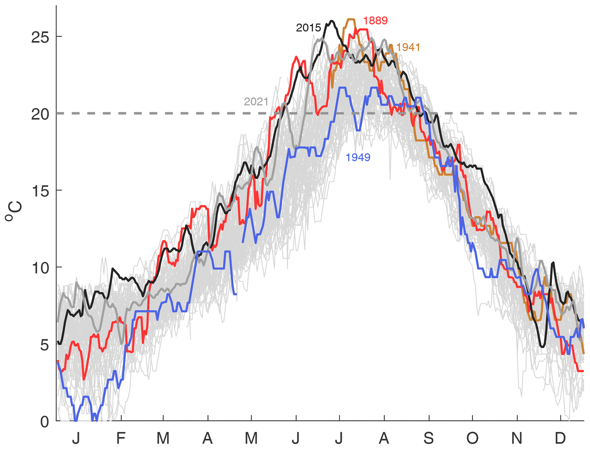
Figure 8Spaghetti plot of all measured Tw data from between 1881–1890 and 1941–2021. Five years (1889, 1941, 1949, 2015, and 2021) are colored as labeled for comparison. The tick marks on the x axis denote the middle of each month.
No single event or individual system perturbation appears to be causing trends, as there are no step-function changes or inflection points in Tw trends (Figs. 6 and 7). Instead, an upwards tendency in Tw is punctuated by large year-to-year variability. In the modern system, the largest interannual variation occurs during the typically high-flow spring months (May–June), with swings of ∼ 5 ∘C observed in bimonthly averages from year to year (Fig. 6). The late-summer and fall season (September–December) is least variable (± 1 ∘C variability between years). During the 19th century, greater year-to-year fluctuations occurred in both measurement and model means during all seasons, typically 4–6 ∘C (Fig. 6). The largest decreases in year-to-year variability are observed between September and February. Cool-season measurements at Astoria (1854–1876) from November–April confirm the historical cool-season variability and track modeled results despite its location on the Columbia River (see, e.g., Figs. 4a, c and 6). The correspondence likely occurs because during fall and winter, proportionally more water in the lower Columbia is sourced from coastal tributaries, especially the Willamette River, than during other times of year (see Naik and Jay, 2011, and Hudson et al., 2017).
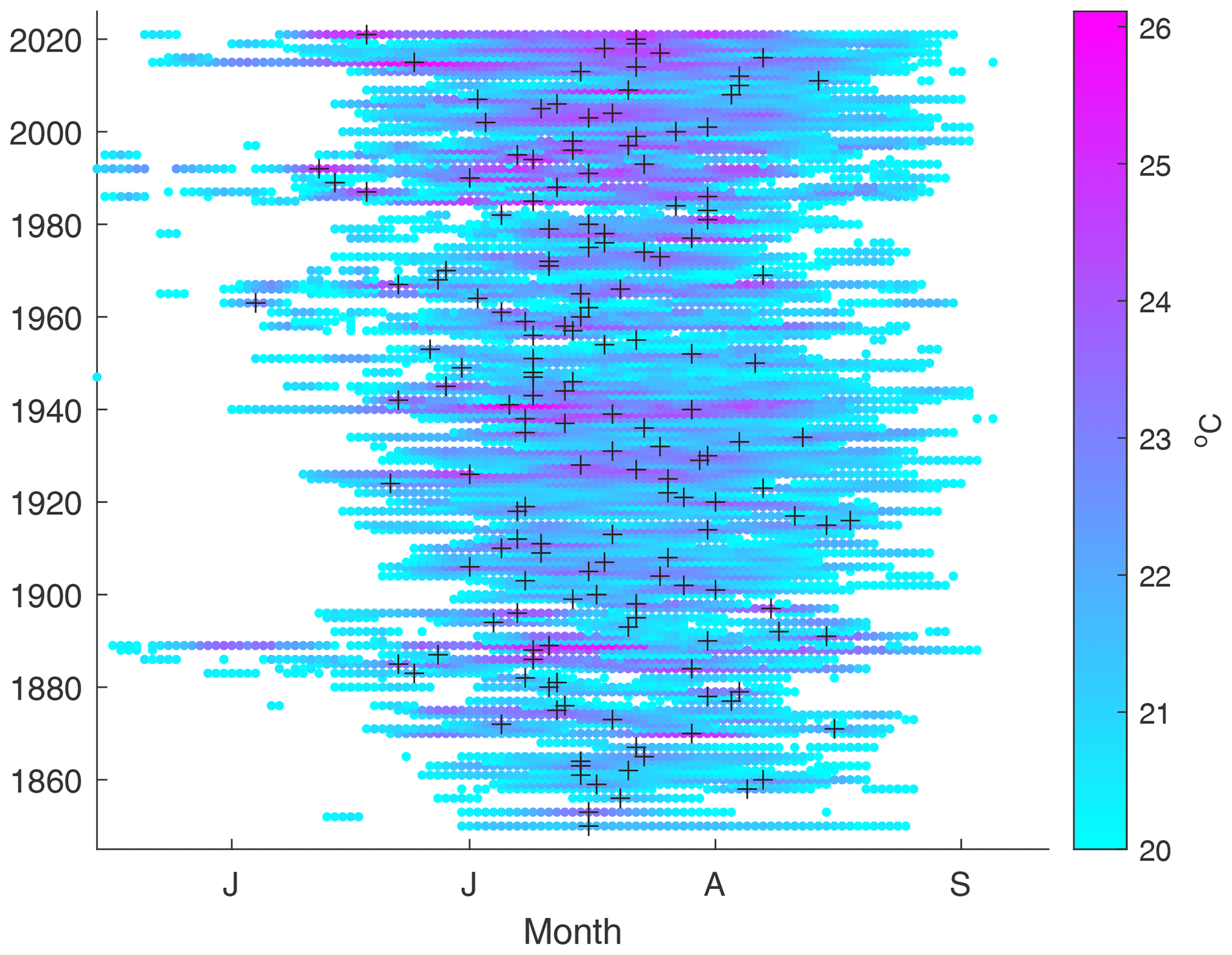
Figure 9Summertime Willamette River Tw exceedances of 20 ∘C, 1850 to 2021. The instrumental record is used between 1881 and 1890 and 1941 to 2021, and the remainder is infilled with modeled Tw. Crosses denote the time of the peak annual Tw. Missing Ta data precluded peak estimates for 1851–1852, 1854–1855, 1857, 1866, and 1868–1869 (see data in the Supplement). The tick marks on the x axis denote the middle of each month.
Results suggest that Tw has exceeded a threshold of 20 ∘C during summer for 15–95 d for the entire 1850–2021 period (Figs. 4, 7c, 8, 9, and 10), despite generally cooler 19th century conditions. A spaghetti plot of all available in situ data shows that maximum Tw and most exceedances of the 20 ∘C Tw threshold occurred in July and August (Fig. 8), with no secular trend in timing observed (Figs. 8 and 9). During some cool summers historically (e.g., 1949; see Fig. 8), Tw oscillated around 20 ∘C during summer. In other years, Tw reaches a peak of 25–26 ∘C and remains above the 20 ∘C threshold from June to September (Figs. 8 and 9). During the hot, low river-discharge summers of 1889 and 2015 (Fig. 8), Tw exceeded 20 ∘C for 91 and 95 d, respectively. The biggest difference between these years, consistent with other observations, is that Tw was more variable during the summer of 1889 than in 2015.
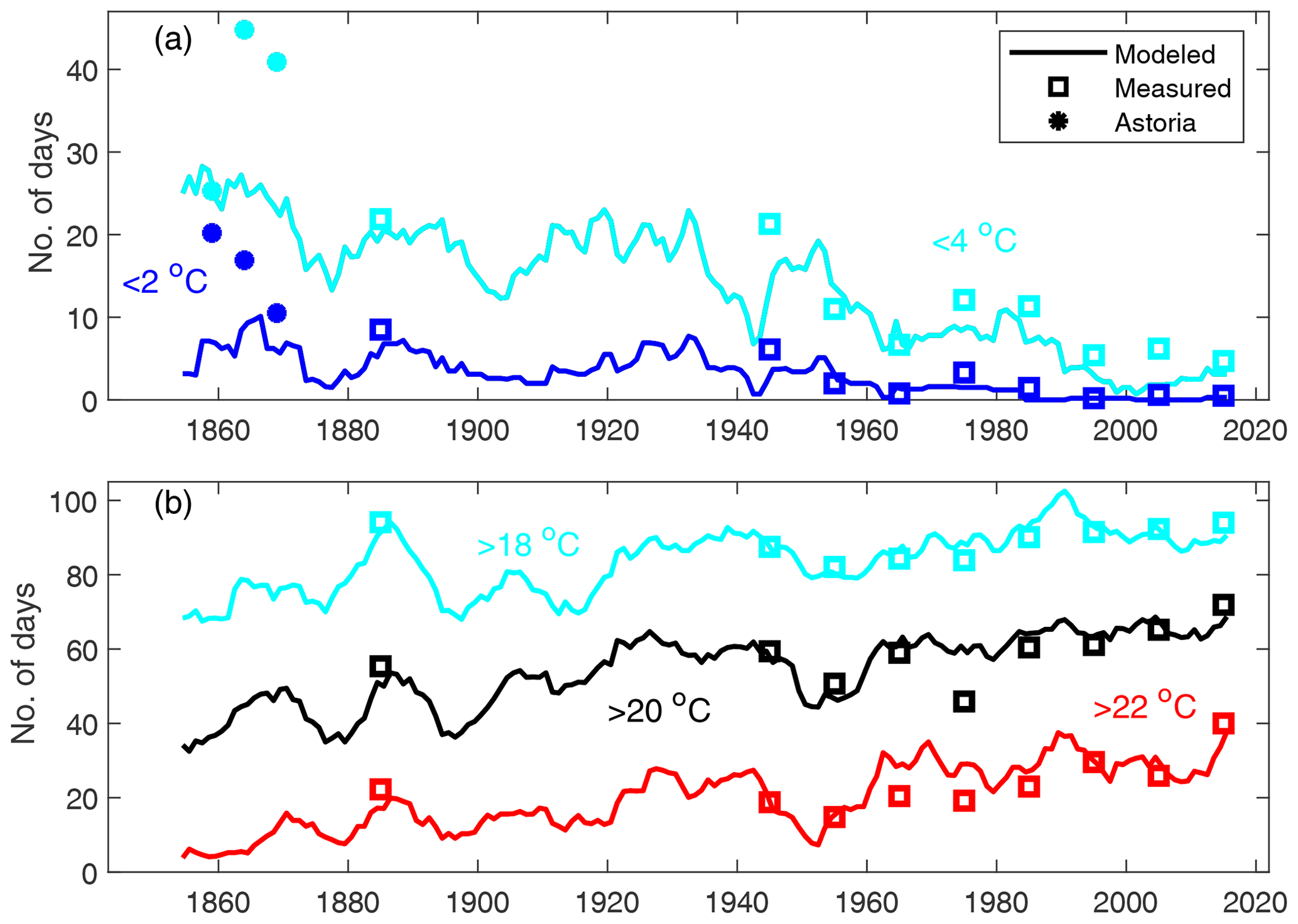
Figure 10Comparison of the modeled and measured number of days per year from 1850 to 2020 that Tw is (a) below thresholds of 2 or 4 ∘C and (b) above thresholds of 18, 20, or 22 ∘C. Square symbols denote the 10-year average based on measurements, while the solid line is a running 10-year average of modeled Tw. Measurements based primarily on bias-corrected upstream gauges (1962, 1983–1984) are excluded. Grey shading is the 95 % confidence interval, based on resampling of model coefficients using a Monte Carlo-based technique. Wintertime measurements from Astoria (1854–1876) are included in (a) for comparison.
Summers with persistently elevated Tw occur more often today than historically (Figs. 8 and 9). On average, Tw crosses the 20 ∘C threshold earlier in the season and exits later than in the 1800s (Fig. 9). From 1881–1890, measurements show that the 7 d average temperature exceeded the effective regulatory limit of 20.3 ∘C (a 0.3 ∘C allowance is added to the 20 ∘C limit; see OR-DEQ, 2006) an average of 42 d, with a range of 11–80 d. For the 2000–2021 period, the range was 35–92 d, with an average of 63 d (see also Fig. 9). Thus, modern measurements show both an increased number of exceedances and a decreased (though still substantial) year-to-year variability. Evaluated using a 10-year average, the number of days per year that exceed 20 ∘C increased by roughly ∼ 50 % (20 d) between 1850 and 2020, from around 40 d yr−1 to more than 60 d yr−1 (Fig. 10). The threshold of 22 ∘C was exceeded relatively rarely in the 1800s (< 5 d yr−1) but is now exceeded nearly 40 d yr−1.
The number of cold-water days in winter has declined as overall temperatures have warmed (Fig. 10a). Tw is now rarely below 4 ∘C, compared to about 25 d yr−1 in the mid-1800s. Similarly, near-freezing temperatures (below 2 ∘C) were common in the 1800s (up to 10 d yr−1) but almost never occur now.
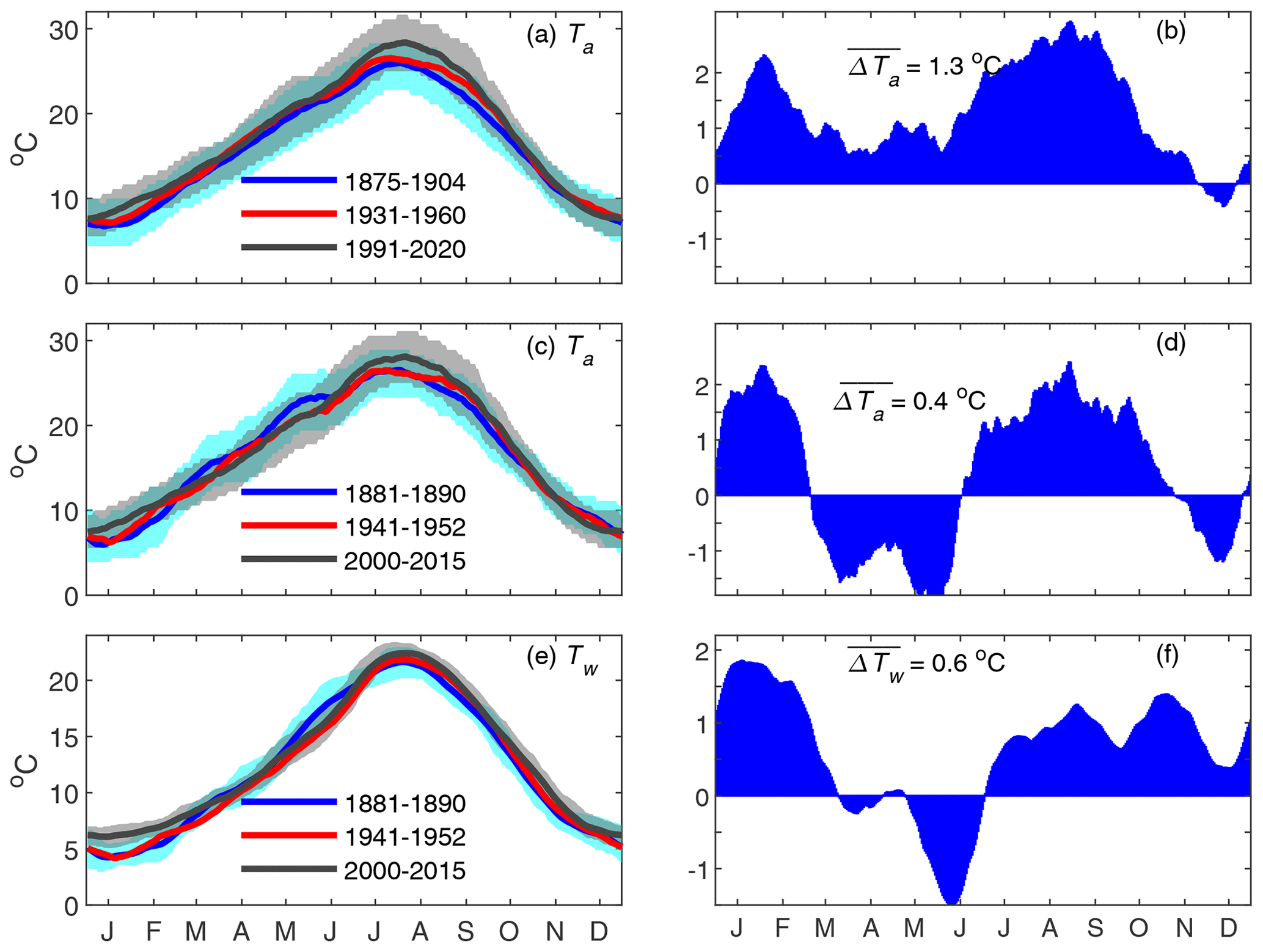
Figure 11Ta and Tw climatology in Portland (a, c, and e) and the corresponding difference between the modern and historical periods (b, d, and e). The Ta difference plot in (b) and (d) is the difference between late 19th and early 21st century air temperature data in (a) and (c), respectively. The difference in (f) is the difference between 2000–2015 and 1881–1890 Tw data. Climatology is determined using a 30 d moving average; shading in (a), (c) and (e) denotes the 25th and 75th percentile of the measurements. A 30-year average is used in (a); the time periods for (c) and (e) are determined by the time period used to calibrate the Tw model. The tick marks on the x axis denote the middle of each month. The average difference between the modern and earliest period is provided in (b, d, and e).
In general, seasonal patterns of measured Tw and shifts between 19th and 21st century data are consistent with measurements of Ta, with some slight variations in timing and magnitude (Fig. 11). Measurements in Portland indicate that average Ta increased by 1.3 ∘C between the 1875–1904 and 1991–2020 periods (based on daily maximum; Fig. 11b), consistent with warming trends of 0.5–2 ∘C per century at 100+ stations throughout the Pacific Northwest (Mote et al., 2003). The smallest increases in Portland Ta occur in spring (April–June) and in late fall (November–December), and the largest occur in January–February and July–October, again consistent with Ta trends in the Maritime Pacific Northwest (Mote, 2003). We find little evidence that the heat-island effect (e.g., Voelkel et al., 2018) is substantially affecting these trends (see the Supplement). Regional air temperature data processed for inferred biases suggest a slightly smaller average change of 0.9 ∘C over a similar period (see Scott et al., 2023), and overall the Pacific Northwest has increased by 1.1 ∘C since 1900 (Mote et al., 2019). Interestingly, the 1880s was an anomalously warm decade for both Ta and Tw; thus, the Ta climatology over a 30-year period shows a greater change between the 19th century and present day (Fig. 11a and b) than the shorter periods of Tw available for calibration (Fig. 11c and d); see the Supplement.
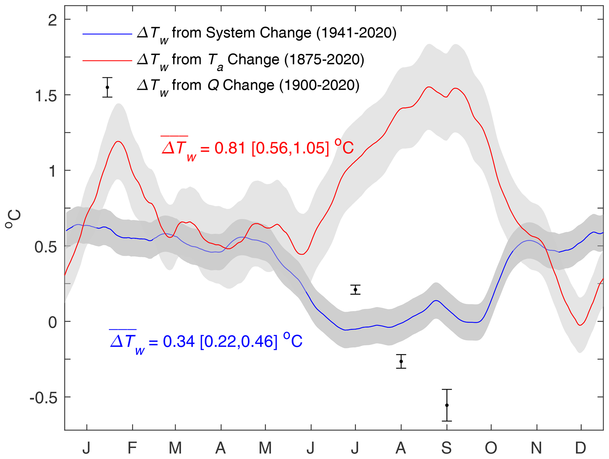
Figure 12Estimated Tw changes caused by Ta (climate change), system changes (i.e., differences between the parameters of the modern and historic models), and discharge changes (July–September). A positive value indicates an increase over time. Shading shows 95 % uncertainty bounds and is a combination of the uncertainty in the mean climatology and the model coefficients. The uncertainty bounds for the influence of altered river flow denote the difference in the 1941A and 2000A model estimates. See Sect. 2.5 for details.
3.3 Causes of water temperature changes
Model sensitivity tests confirm that changes in Ta driven by climate change are the most significant factor in long-term increases in Tw, with net river system changes an additional important contributor during the cool season (see Sect. 2.5, Fig. 12). Seasonally, changes in Ta between the 1875–1904 and 1991–2020 periods dominate the modeled trends in Tw during late winter, summer, and early fall (late January–early March, July–October; Fig. 12). Averaged over a year, a total increase in Tw of 0.81 ± 0.25 ∘C is correlated to Ta changes. A maximum climate-induced Tw change of ∼ 1.7 ± 0.3 ∘C occurs in September. Climate shifts produce a lesser shift of 0.5–0.6 ∘C increase in Tw in spring (late March to June), and little change occurs in December, consistent with air temperature climatology (compare Figs. 11 and 12). The uncertainty in the Ta contribution is driven by the uncertainty in the Ta climatological average, which is ± 0.22 ∘C and is caused by interannual variability (see Eq 5); model coefficient uncertainty is a minor factor. Modeled Tw changes are robust to small systematic biases in Ta; if the average change in Ta is reduced by 0.4 ∘C (consistent with the Scott et al., 2023, estimate for Portland Ta change), the average Tw only decreases by ∼ 0.23 ∘C. Hence, we conclude that changes in the meteorological heat balance (as represented by Ta) are the major cause of increasing Tw.
Integrated system changes between the 1940s and today (defined in Sect. 2.5) cause a Tw increase of ∼ 0.5–0.6 ∘C from November–May but are statistically insignificant from late June to early October (Fig. 12). Averaged over a year, the total increase in Tw caused by system change is 0.34 ± 0.12 ∘C since the 1940s; no statistically significant change between the 1881 and 1941 era models was found. The net change of 0.34 ∘C is caused by an altered decorrelation structure between models from the 2000 and 1941 eras (Fig. 3).
Changes in the average river hydrograph (Fig. 2a) are important for Tw during late summer. During July, a slight increase in Tw is observed from changed river flow. In August and especially September, the decreases in Tw caused by increased flow releases are significant (−0.27 and −0.56 ∘C, respectively). Thus, the release of water from reservoirs late in the summer to some extent counteracts the effects of increased air temperatures (Fig. 12). During other times of year, no statistically significant modeled correlation between Q and Tw was found, likely because the average Tw gradient in the mainstem Willamette River is small (Fig. 2b). While river flow may be important in winter during times of large positive or negative temperature gradients, these changes are likely transient, and a process-based model would be required to detect them. The net effect of summertime changes in Q on the annual average is small: a total decrease in annually averaged Tw of ∼ 0.05 ∘C is estimated.
The observed annual trend in Tw of 1.1 ± 0.2 ∘C per century in the lower Willamette River is similar to the magnitude of change observed or estimated in the few studies available over similar timescales. For example, Moatar and Gailhard (2006) estimated a 0.8 ∘C increase in the Loire since 1881, Webb and Nobilis (2007) estimated a change of 1.4–1.7 ∘C in Austrian rivers since ∼ 1900, and Scott et al. (2023) estimated a trend of 1.3 ∘C per century for the Columbia River over the past 170 years. Similar to our results, studies also often highlight that the seasonal distribution of changes of Tw is uneven (e.g., Webb and Nobilis, 2007). Consistent with our results, studies from the Pacific Northwest suggest that the processes driving increased Ta (i.e., climate change) have also been driving Tw trends over recent decades (Isaak et al., 2012). Future climate change is expected to continue to increase Ta and drive Tw trends, with the largest increases in summer (Caldwell et al., 2013; Ficklin et al., 2014). Additionally, unimpeded discharge is expected to increase in winter and decrease in summer (e.g., Chang and Jung, 2010), which would also raise late summer Tw (Fig. 12).
4.1 Interpretation of Tw patterns
Ongoing air temperature changes are the primary cause of the modeled increase in water temperatures, with river system changes an important contributor (Fig. 12). The sum of estimated temperature changes caused by climate, system, and water management changes from ∼ 1900 to present is ∼ 1.1 ± 0.3 ∘C (Fig. 12) and is consistent with the overall long-term trends in Tw of 1.1 ± 0.2 ∘C per century (Fig. 7a). Of modeled changes since ∼ 1900, 0.81 ± 0.25 ∘C (74 %) is caused by increased Ta, while 0.34 ± 0.12 ∘C (∼ 31 %) is caused by alterations in the Tw response to forcing (integrated river system change); river flow alteration produces a −5 % change, closing the balance. Thus, we conclude that the largest increases in Willamette water temperature are driven by climate change. This contrasts with the nearby Columbia River, in which flow regulation and other anthropogenic changes cause the majority of historical Tw shifts (Scott et al., 2023). One major difference is the percentage of water that is stored in reservoirs: approximately 40 % of Columbia River flow is stored behind reservoirs vs. about 10 % for the Willamette.
Our results suggest that deepening of the river system has altered the response of Tw to meteorological forcing and weather extremes, producing less water temperature variance (Figs. 5 and 6) and an altered decorrelation structure in model coefficients (Fig. 3). At short time lags of 0–5 d, historical model coefficients are as much as 2–3 times larger than modern coefficients, indicating more sensitivity to air temperature fluctuations (Fig. 3). In the modern system, increased depth d compared to historical conditions reduces the effect of atmospheric heating H, leading to smaller and smaller coefficients (see Eq 1; Caissie, 2006). Depth increases are driven by the reservoir system (e.g., Rounds, 2007), which is known to decrease Tw variability in the Willamette on 1–8 d timescales (Steel and Lange, 2007). The change from braided, shallow channels to a single, deeper channel is also likely influential (see Sect. 2.1 and Sedell and Froggatt, 1984).
The changing correlation structure (Fig. 3) and the influence of increasing depth have implications for how extremes occur in a changing climate. Specifically, a historical heat wave in Ta was likely to produce a larger change in Tw than it would today. The record-breaking, climate-change-influenced heat wave in July 2021 (e.g., White et al., 2023), with a high Ta of 46.7 ∘C, did not cause a record Tw. Despite Ta values exceeding the previous all-time high by nearly 5 ∘C, morning water temperature peaked at just over 24 ∘C, approximately 2 ∘C below the largest recorded (as discussed in Sect. 2.2, we use morning measurements in our model). A similar process mitigates the effect of cold air events and helps keep modern water temperatures above freezing (Fig. 7). Effectively, Tw in the modern river system has become more resilient to extreme heat waves or cold weather anomalies.
Another reason for historical Tw variability in winter was the occasional occurrence of deep freezes that no longer occur. During the winters of 1861–1862 and 1867–1868, for example, Ta remained below 0 ∘C for 32 and 31 d, respectively, and newspapers recorded ice-skating on the lower Willamette River. Navigation in Portland Harbor was halted or hindered by ice from New Year's Day until mid-March 1862. No 20th century winter matched the duration or severity of these events, though 18–19 freezing days (daily maximum below 0 ∘C) were recorded in 1915–1916, 1929–1930, and 1949–1950. In 1979, air temperatures remained below 0 ∘C for a total of 14 d; since 1980, no winter has produced more than 9 sub-freezing days. On average, the statistical variability of air temperature from its climatological mean is similar today to that historically (Fig. 5); however, the frequency of extremely cold waves (e.g., 1- in 10-year events) has decreased over the past century (Vose et al., 2017). The average coldest day of the year is now ∼ 2.7 ∘C warmer in the Pacific Northwest than during the first half of the 20th century, far outpacing the annual average increase of 1.1 ∘C since 1900 (Vose et al., 2017, Mote et al., 2019). Both increasing average winter air temperatures and decreasing cold extremes help explain upward trends in bimonthly averaged temperatures (Fig. 6) and seasonal minima (Fig. 7b). For example, the year-to-year variation in average January–February Tw was 0–6 ∘C during the 19th century and is 5–8 ∘C today (Fig. 6). During winter, the shallower historical streams may have contributed to the ice formation observed during some 19th century winters. Thus, changing meteorological forcing combines together with altered system response to increase wintertime temperatures but reduce variance (Fig. 12).
The integrated effect of weather during previous months is more important today than historically. At lags of > 2 weeks, coefficient magnitudes are ∼ 50 % larger in the modern models (see Sect. 3.1). Hence, the thermal memory of the system to Ta anomalies lasting a month or longer is larger. Nonetheless, the influence of each individual day at lags > 2 weeks is small (see Fig. 30), and only the integrated, monthly averaged effect is important. Hence, increased thermal memory smooths out variability and keeps the system closer to climatological conditions. Thermal memory (thermal inertia) also elevates wintertime and depresses early-summertime temperatures (e.g., Fig. 12). Similar patterns have been observed elsewhere and attributed to water regulation and storage (see, e.g., Webb and Walling, 1993; Caissie, 2006; Olden and Naiman, 2010) but can also be influenced by the time-lag effects of snowmelt.
Numerical, process-based models run over a shorter duration provide additional clues to the factors driving long-term changes. For example, loss of shading (86 %) and point-source discharges (∼ 14 %) increased Willamette River temperatures in Portland by 0.3 ± 0.05 ∘C between June and October 2001 (OR-DEQ, 2006). The same numerical model determined a reduction of approximately 0.1 ∘C for each additional 100 m3 s−1 of river flow released into the lower Willamette. This is consistent though not identical with our modern statistical model, which produces an average decrease of −0.07 ∘C for each extra 100 m3 s−1 of river flow.
River discharge is found to only be influential on Tw during summer (see also Isaak et al., 2012) and is driven by the substantial increase in water temperature along the river observed during July–September (positive ; Fig. 2b). Another factor is the increased velocity u and river depth d caused by regulated releases of water. Larger river flow increases the rate at which cooler water is moved downstream (increased ) and increased depth diminishes the contribution from surface heating on temperature (smaller ; see Eq. 1). The large increase in September discharge compared to historical conditions (Fig. 2) reduces temperatures by 0.56 ∘C, more than in August (Fig. 12). In October, average becomes small (Fig. 2), and managed releases are unlikely to reduce water temperature, on average. After September, our approach is unable to find a statistically significant influence of river discharge.
Interestingly, the overall river system was less sensitive to river flow fluctuations in the 1940s (Fig. 3d), and no statistically significant effect of river flow was observed in the 1880s. The lack of correlation in the 1880s may simply reflect incomplete flow estimates (see Jay and Naik, 2011). A dynamical explanation remains speculative without a process-based retrospective model using historical bathymetry. However, some factors may have reduced average summertime river flow influences () historically (Eq. 1). Compared to today, the bottomland forests and braided river networks of the historical Willamette River probably reduced velocity u, and the longer river length slightly reduces (see Sect. 2.1). Cold groundwater discharges, which are known to occur in off-main channel alcoves and were more connected to the river historically (e.g., Faulkner et al., 2020), may have reduced surface heating effects. Riparian shading and smaller watershed stream widths similarly reduced heating (OR-DEQ, 2006; White et al., 2017). Nonetheless, understanding the relative importance of these factors requires additional research.
4.2 Implications
The increase in the number of days that water temperatures exceed established thresholds has been observed in other river systems (e.g., Markovic et al., 2013) and is projected to continue in the Pacific Northwest (Mantua et al., 2010). Our observations show that the rate of change is threshold-dependent and slows as the accumulated number of days above a threshold becomes large. Therefore, the number of days over 20 ∘C (which is already large) is increasing less quickly than the number of days over 22 ∘C, which occur primarily during mid-summer (Fig. 9). Effectively, exceedances of lower thresholds like 18 and 20 ∘C are limited by spring and fall, when climatological values of Ta and Tw change quickly (note that springtime Tw is also held lower by thermal memory). Conversely, in winter, the largest rates of change are observed for larger levels of exceedance; hence, the number of cold-water days below 4 ∘C is decreasing faster than those below 2 ∘C. Both the decreased spread in water temperatures (Fig. 5) and increased mean temperatures (Fig. 6 and 7) drive the large change in the number of days below 4 ∘C. Increases in winter Tw minima and averages are not a focus of regulation but are ecologically important (e.g., Webb and Weber, 1993; Caissie, 2006). For example, cold-water events and wintertime conditions influence the survivability and recruitment of fish by altering their biotic interactions, habitat use, physical condition, feeding rates, and community structure (see reviews by Hurst, 2007; Brown et al., 2011; Weber et al., 2013). It is also possible that historical wintertime conditions, such as the deep freezes discussed above, provided some protection against non-native plants and fauna that thrive in warmer waters.
Compared to historical norms, Tw today exhibits lower variability, both day-to-day and between annual maximum and minimum values. A result is that temporal refugia – which we define as time periods in which Tw temporarily dips below biologically important thresholds such as 18 or 20 ∘C – are becoming less frequent (see Figs. 9 and 10). Hence, while the management practice of selectively releasing river water is successfully reducing average temperatures in late summer (Fig. 12), it may not be addressing the decrease in variance (e.g., Fig. 5) caused by system changes. Because some migrating fish such as steelhead delay migration during warm periods by weeks or months, likely causing increased mortality (e.g., Siegel et al., 2021), a reduction in temporal refugia is potentially important (see also Steel et al., 2012). At Portland, Tw exceeds biologically important thresholds during some part of every year and did so even in the 19th century. However, the more consistently warm river temperatures during summer and fall – as observed by the increase in time over 18 and 20 ∘C – likely creates a thermal barrier, with implications for salmon migration (see, e.g., Notch et al., 2020).
4.3 Study limitations
Statistical models are fast, can be applied over long time periods, and provide insights into the major factors influencing water temperature (e.g., Benyahya et al., 2007). Nonetheless, factors such as wind, heating, evaporation, time or spatial variation in parameters, and alterations in depth are only approximately represented by Ta and Q. At different times, various terms (e.g., depth, heat flux, and velocity) may contribute in varying degrees to the overall heat balance (Eq. 1), leading to a different statistical relationship between forcing variables and Tw. We address this issue by developing summer, winter, and annual sub-models and by developing models for different eras (Fig. 3). Nonetheless, river system and climate changes occurred continuously over the period of record, making application of the models to different time periods only approximate. For example, managed releases of water for temperature control became more prevalent in the late 1990s (National Research Council, 2004) and may decrease the hindcast skill of our 2000 era model for earlier periods. The quality and spatial variability of input data used in the model may also affect conclusions. If we use a 0.9 ∘C increase in air temperature since 1900 (following Scott et al., 2023), rather than 1.3 ∘C, the estimated average influence of Ta on Tw is reduced by 0.23 ∘C in Fig. 12. Nonetheless, our results are generally consistent between models (Sect. 3.1), and any small biases or uncertainties in the data only shift the details, but not the main conclusions, of the study.
Our approach cannot discern the influence of individual factors such as altered shading, river depth, storage, or snowpack, nor can we assess coupled, nonlinear changes. For example, changes in river flow (Fig. 2) may be caused jointly by climate change, land-use change, and water management change (e.g., Swain et al., 2021, Liang et al., 2020), and alterations in Ta can be influenced by urbanization or deforestation. A numerical modeling approach is needed to isolate individual anthropogenic stressors and to determine how landscape and climate changes can influence Tw in incremental, nonlinear, and interdependent ways (e.g., Berger et al., 2004). Nonetheless, our results provide insights into the causes of Tw change and why some parts of the year are subject to larger upward trends than others, over secular timescales.
In this contribution, we found, digitized, produced, and quality-controlled a 90-year-long Tw record (1881–2021) for the lower Willamette River in Portland, Oregon. The in situ measurements enabled the development of statistical Tw models based on the 1880s, 1940s, and modern time periods. Subsequently, estimates of daily minimum Tw for the years 1850–2021 were produced using daily measurements of maximum Ta and river discharge. A good comparison between measurements and models is observed, with an RMSE similar to numerical models.
Water temperatures are increasing throughout the year (average trend of 1.1 ± 0.2 ∘C per century), with the largest increase observed in winter. As a result, the number of cold-water days per year is declining, while the number of days above 20 ∘C has increased by an average of ∼ 20 d yr−1. The primary cause of changed Tw since 1900 is climate change (0.84 ∘C), followed by system changes such as the building of reservoirs, loss of shading, and other landscape alterations (0.34 ∘C). Changes in river discharge have a generally smaller influence, except during managed releases in late summer.
Ongoing climate changes (as observed through air temperature increases) are the primary cause of increased water temperatures, with river system changes an important contributor, particularly during winter. Because of a larger heat capacity and greater system depth, the day-to-day variability in Tw has decreased, and the sensitivity to meteorological heat waves or cold waves is diminished. These changes are observed in model coefficients and in a reduced variance from the climatological mean. Thus, average temperatures in summer are now higher than historically and have increased more rapidly than annual maxima. Hence, warm summers marked by low river flow produced similar peak temperatures in 1889, 1941, and 2015, but an extreme heat wave in 2021 did not produce record Tw values. River system alterations and climate change have greatly increased winter water temperatures and reduced year-to-year variability, and meteorologically induced disturbance events such as freezing rarely occur anymore. Similarly, temporal refugia – time periods in which Tw dips below biologically important warm water thresholds – have also decreased. These system changes may contribute to the threat to endemic species, particularly if climate-induced changes in Tw continue.
The Tw data have been archived in the Portland State University data depository (https://doi.org/10.15760/cee-data.06, Talke et al., 2023). Meteorological data are available from the National Centers for Environmental Information (https://www.ncei.noaa.gov/, NCEI, 2021). Pre-1890 Vancouver and Portland records were also obtained from the Midwestern Regional Climate Center (https://mrcc.purdue.edu/; MRCC, 2023). River flow records are obtained from the US Geological Survey and the sources described in Sect. 2.2.
The supplement related to this article is available online at: https://doi.org/10.5194/hess-27-2807-2023-supplement.
SAT found and processed archival data, conceptualized research question, developed the statistical model, analyzed results, produced figures, and was primary lead on drafting the paper. DAJ developed an earlier version of the model and assisted with research questions, interpretation, and paper development. HLD assisted with conceptualizing research questions, interpretation, literature review, and paper development.
The contact author has declared that none of the authors has any competing interests.
Publisher's note: Copernicus Publications remains neutral with regard to jurisdictional claims in published maps and institutional affiliations.
Funding was provided by Bonneville Power Administration, under project no. 2002-077-00 with the Pacific Northwest National Laboratory, and by the US National Science Foundation, CAREER Award 1455350 and NSF project 2013280. Margaret McKeon is thanked for her help defining the watershed boundaries in Fig. 1, and students at Portland State University are thanked for helping to digitize and quality-assure the 1854–1876, 1881–1890, and 1941–1961 Tw records used in this study.
This research has been supported by the National Science Foundation, Directorate for Geosciences (grant nos. 1455350 and 2013280), and the Bonneville Power Administration (grant no. 2002-077-00).
This paper was edited by Jan Seibert and reviewed by two anonymous referees.
Al-bahadily, A.: Long Term Changes to the Lower Columbia River Estuary (LCRE) Hydrodynamics and Salinity Patterns, PhD thesis, Portland State University, https://doi.org/10.15760/etd.7357, 2020.
Al-Murib, M. D., Wells, S. A., and Talke, S. A.: Integrating Landsat TM/ETM+ and numerical modeling to estimate water temperature in the Tigris River under future climate and management scenariosm, Water, 11, 892, https://doi.org/10.3390/w11050892, 2019.
Angilletta M. J., Steel E. A., Bartz K. K., Kingsolver J. G.,Scheurell M. D., Beckman B. R., and Crozier L. G.: Big dams and salmon evolution: changes in thermal regimes and their potential evolutionary consequences, Evol. Appl., 1, 286–299, https://doi.org/10.1111/j.1752-4571.2008.00032.x, 2008.
Annear, R., McKillip, M., Khan, S. J., Berger, C., and Wells, S.: Willamette Basin Temperature TMDL Model: Boundary Conditions and Model Setup, Technical Report EWR-03-03, Department of Civil and Environmental Engineering, Portland State University, Portland, Oregon, 2003.
Baker, J., Van Sickle, D., White, D.: Water Sources and Allocation, in: Willamette River Basin Planning Atlas, edited by: Hulse, D., Gregory, S., and Baker, J., Oregon State University Press, Corvallis, 40–43, ISBN 10 0870715429, 2002.
Benner, P. and Sedell, J.: Upper Willamette River Landscape: A Historic Perspective, in: River Quality: Dynamics and Restoration, edited by: Laenen, A. and Dunnette, D. A., CRC/Lewis, Boca Raton, 23–46, ISBN 9780203740576, https://doi.org/10.1201/9780203740576, 1997.
Benyahya L., Caissie, D., St-Hilaire, A., Ouarda, T. B. M. J., and Bobée, B.: A Review of statistical water temperature models, Can. Water Resour. J., 32, 179–192, https://doi.org/10.4296/cwrj3203179, 2007.
Berger, C., McKillip, M. L., Annear, R. L., Khan, S. J., and Wells, S. A.: Willamette Basin Temperature TDML Model: Model Calibration, Technical Report EWR-02-04, Department of Civil and Environmental Engineering, Portland State University, Portland, OR, https://pdxscholar.library.pdx.edu/cgi/viewcontent.cgi?article=1162&context=cengin_fac (last access: 13 July 2023), 2004.
Bottom, D., Baptista, A., Burke, J., Campbell, L., Casillas, E., Hinton, S., Jay, D. A., Lott, M. A., McCabe, G., McNatt, R., Ramirez, M., Roegner, G. C., Simenstad, C. A., Spilseth, S., Stamatiou, L., Teel, D., and Zamon, J. E.: Estuarine habitat and juvenile salmon: Current and historical linkages in the Lower Columbia River and estuary, Final report, 2002–2008, Report of the National Marine Fisheries Service to the U.S. Army Corps of Engineers, Portland, Oregon, https://www.fisheries.noaa.gov/resource/publication-database/northwest-fisheries-science-center-publications-database (last access: 13 July 2023), 2011.
Branscomb, A., Goicochea J., and Richmond, M.: Stream Network, in: Willamette River Basin Planning Atlas, edited by: Hulse, D., Gregory, S., and Baker, J., Oregon State University Press, Corvallis, 16–17, ISBN 10 0870715429, 2002.
Brooks, J. R., Wigington, P. J., Phillips, D. L., Comeleo, R., and Coulombe, R.: Willamette River Basin surface water isoscape (δ18O and δ2H): temporal changes of source water within the river, Ecosphere, 3, 39, https://doi.org/10.1890/ES11-00338.1, 2012.
Brown, R. S., Hubert, W. A., and Daly, S. F.: A primer on winter, ice, and fish: what fisheries biologists should know about winter ice processes and stream-dwelling fish, Fisheries, 36, 8–26, https://doi.org/10.1577/03632415.2011.10389052, 2011.
Bumbaco, K. A., Dello, K. D., and Bond, N. A.: History of Pacific Northwest Heat Waves: Synoptic Pattern and Trends, J. Appl. Meteorol. Clim., 52, 1618–1631, https://doi.org/10.1175/JAMC-D-12-094.1, 2013.
Caissie, D.: The thermal regime of rivers: a review, Freshwater Biol., 51, 1389–1406, https://doi.org/10.1111/j.1365-2427.2006.01597.x, 2006.
Caissie, D., El-Jabi, N., and St-Hilaire, A.: Stochastic Modelling of water temperatures in a Small Stream Using Air to Water Relations, Can. J. Civil Eng., 25, 250–260, https://doi.org/10.1139/l97-091, 1998.
Caldwell, R. J., Gangopadhyay, S., Bountry, J., Lai, Y., and Elsner, M. M.: Statistical modeling of daily and subdaily stream temperatures: Application to the Methow River Basin, Washington, Water Resour. Res., 49, 4346–4361, https://doi.org/10.1002/wrcr.20353, 2013.
Chang, H. and Jung, I. W.: Spatial and temporal changes in runoff caused by climate change in a complex large river basin in Oregon, J. Hydrol., 388, 186–207, https://doi.org/10.1016/j.jhydrol.2010.04.040, 2010.
Christy, J. A. and Alverson, E. R.: Historical vegetation of the Willamette Valley, Oregon, circa 1850, Northwest Sci., 85, 93–107, https://doi.org/10.3955/046.085.0202, 2011.
Clemens, B., Schreck, C., van de Wetering, S., and Sower, S.: The potential roles of river environments in selecting for stream- and ocean-maturing Pacific lamprey, Entosphenus tridentatus (Gairdner, 1836), in: Jawless fishes of the world, Volume 1, edited by: Orlov, A. and Beamish, R., Cambridge Scholars Publishing, Newcastle upon Tyne, UK, 299–322, 2016.
Clemens, B. J.: Warm water temperatures (≥ 20 ∘C) as a threat to adult Pacific lamprey: Implications of climate change, J. Fish Wildl. Manag., 13, 1–8, https://doi.org/10.3996/JFWM-21-087, 2022.
Cloern, J. E., Knowles, N., Brown, L. R., Cayan, D., Dettinger, M. D., Morgan, T. L., Schoellhamer, D. H., Stacey, M. T., van der Wegen, M., Wagner, R. W., and Jassby, A. D.: Projected evolution of California's San Francisco Bay-Delta-River System in a century of climate change, PLoS ONE, 6, e24465, https://doi.org/10.1371/journal.pone.0024465, 2011.
Crozier, L. G., Siegel, J. E., Wiesebron, L. E., Trujillo, E. M., Burke, B. J., Sandford, B. P., and Widener, D. L.: Snake River sockeye and Chinook salmon in a changing climate: implications for upstream migration survival during recent extreme and future climates, PLOS ONE, 15, e0238886, https://doi.org/10.1371/journal.pone.0238886, 2020.
Donato, M. M.: A Statistical Model for Estimating Stream Temperatures in the Salmon and Clearwater River Basins, Central Idaho, US Geological Survey Water Resources Investigations Report 2002-4195, US Geological Survey, https://doi.org/10.3133/wri024195, 2002.
Dugdale, S. J., Hannah, D. M., and Malcolm, I. A.: River temperature modelling: a review of process-based approaches and future directions, Earth Sci. Rev., 175, 97–113. https://doi.org/10.1016/j.earscirev.2017.10.009, 2017.
Faulkner B. R., Brooks J. R., Keenan D. M., and Forshay K. J.: Temperature Decrease along Hyporheic Pathlines in a Large River Riparian Zone, Ecohydrology, 13, 1–10, https://doi.org/10.1002/eco.2160, 2020.
Feigl, M., Lebiedzinkski, K., Herrnegger, M., and Schulz, K.: Machine-learning methods for stream water temperature prediction Hydrol. Earth Syst. Sci., 25, 2951–2977, https://doi.org/10.5194/hess-25-2951-2021, 2021.
Ficklin, D. L., Barnhart, B. L., Knouft, J. H., Stewart, I. T., Maurer, E. P., Letsinger, S. L., and Whittaker, G. W.: Climate change and stream temperature projections in the Columbia River basin: habitat implications of spatial variation in hydrologic drivers, Hydrol. Earth Syst. Sci., 18, 4897–4912, https://doi.org/10.5194/hess-18-4897-2014, 2014.
Fischer, H. B., List, E. J., Koh, R. C. Y., Imberger, J., and Brooks, N. H.: Mixing in inland and coastal waters, Academic, New York, ISBN 978-0-08-051177-1, https://doi.org/10.1016/C2009-0-22051-4, 1979.
Gregory, S., Wildman, R., Hulse, D., Ashkenas, L., and Boyer, K.: Historical changes in hydrology, geomorphology, and floodplain vegetation of the Willamette River, Oregon, River Res. Appl., 35, 1279–1290, https://doi.org/10.1002/rra.3495, 2019.
Gregory, S., Ashkenas, L., Oetter, D., Minear, P., and Wildman, K.: Historical Willamette River Channel Change, in: Willamette River Basin Planning Atlas, edited by: Hulse, D., Gregory, S., and Baker, J., Oregon State University Press, Corvallis, 18–25, ISBN 10 0870715429, 2002a.
Gregory, S., Ashkenas, L., Oetter, D., Wildman, R., Minear, P., Jett, S., and Wildman, K.: Revetments, in: Willamette River Basin Planning Atlas, edited by: Hulse, D., Gregory, S., and Baker, J., Oregon State University Press, Corvallis, 32–33, ISBN 10 0870715429, 2002b.
Gregory, S., Ashkenas, L., Jett, S., and Wildman, R.: Flood inundations/FEMA floodplains, in: Willamette River Basin Planning Atlas, edited by: Hulse, D., Gregory, S., and Baker, J., Oregon State University Press, Corvallis, 28–29, ISBN 10 0870715429, 2002c.
Gregory, S., Ashkenas L., Oetter,D., Minear, P., Wildman, K., Christy, J., Kolar, S., and Alverson, E.: Presettlement Vegetation ca. 1851, in: Willamette River Basin Planning Atlas, edited by: Hulse, D., Gregory, S., and Baker, J., Oregon State University Press, Corvallis, 38–39, ISBN 10 0870715429, 2002d.
Gregory, S. V., Frederick, J., Swanson, W., McKee, A., and Cummins, K. W.: An Ecosystem Perspective of Riparian Zones: Focus on links between land and water, BioScience, 41, 540–551, https://doi.org/10.2307/1311607, 1991.
Hamlet, A. F. and Lettenmaier, D. P.: Effects of climate change on hydrology and water resources in the Columbia River Basin, J. Am. Water Resour. As., 35, 1597–1623, https://doi.org/10.1111/j.1752-1688.1999.tb04240.x, 1999.
Helaire, L. T., Talke, S. A., Jay, D. A., and Mahedy, D.: Historical changes in Lower Columbia River and Estuary Floods and Tides, J. Geophys. Res., 124, 7926–7946, https://doi.org/10.1029/2019JC015055, 2019.
Hudson, A. S., Talke, S. A., and Jay, D. A.: Estuaries and Coasts Using satellite observations to characterize the response of estuary turbidity maxima to external forcing, Estuar. Coast., 40, 343–358, https://doi.org/10.1007/s12237-016-0164-3, 2017.
Hurst, T. P.: Causes and consequences of winter mortality in fishes, J. Fish Biol., 71, 315–345, https://doi.org/10.1111/j.1095-8649.2007.01596.x, 2007.
Isaak, D. J., Wollrab, S., Horan, D., and Chandler, G.: Climate change effects on stream and river temperatures across the northwest U.S. from 1980–2009 and implications for salmonid fishes, Climatic Change, 113, 499–524, https://doi.org/10.1007/s10584-011-0326-z, 2012.
Jay, D. A. and Naik, P. K.: Distinguishing Human and Anthropogenic Influences on Hydrological Disturbance Processes in the Columbia River, USA, Hydrolog. Sci. J., 56, 1186–1209, https://doi.org/10.1080/02626667.2011.604324, 2011.
Johnson S. L. and Jones J. A.: Stream temperature response to forest harvest and debris ?ows in western Cascades, Oregon, Can. J. Fish. Aquat. Sci., 57, 30–39, https://doi.org/10.1139/cjfas-57-S2-30, 2000.
Kaushal, S. S., Likens, G. E., Jaworski, N. A., Pace, M. L., Sides, A. M., Seekell, D., Belt, D. H., Secor, R. L., and Wingate, R. L.: Rising stream and river temperatures in the United States, Front. Ecol. Environ., 8, 461–466, https://doi.org/10.1890/090037, 2010.
Kinouchi, T.: Impact of long-term water and energy consumption in Tokyo on wastewater effluent: implications for the thermal degradation of urban streams, Hydrol. Process., 21, 1207–1216, https://doi.org/10.1002/hyp.6680, 2007.
Knowles, N. and Cayan, D.: Potential Effects of Global Warming on the Sacramento/SanJoaquin Watershed and the San Francisco Estuary, Geophys. Res. Lett., 29, 38-1–38-4, https://doi.org/10.1029/2001GL014339, 2002.
Landers, D., Fernald, A., and Andrus, C.: Off-channel Habitats, in: Willamette River Basin Planning Atlas, edited by: Hulse, D., Gregory, S., and Baker, J., Oregon State University Press, Corvallis, 26–27, ISBN 10 0870715429, 2002.
Lee, K.: Stream Velocity and Dispersion Characteristics Determined by Dye-Tracer Studies on Selected Stream Reaches in the Willamette River Basin, Oregon, U.S. Geological Survey Water-Resources Investigations Report 95-4078, U.S. Geological Survey, https://pubs.er.usgs.gov/publication/wri954078 (last access: 13 July 2023), 1995.
Liang, S., Wang, W., Zhang, D., Li, Y., and Wang, G.: Quantifying the impacts of climate change and human activities on runoff variation: case study of the upstream of Minjiang River, China, J. Hydrol. Eng., 25, 05020025, https://doi.org/10.1061/(ASCE)HE.1943-5584.0001980, 2020.
Mantua, N., Tohver, I., and Hamlet, A.: Climate change impacts on streamflow extremes and summertime stream temperature and their possible consequences for freshwater salmon habitat in Washington State, Climatic Change, 102, 187–223, https://doi.org/10.1007/s10584-010-9845-2, 2010.
Markovic, D., Scharfenberger, U., Schmutz, S., Pletterbauer,F., and Wolter, C.: Variability and alterations of water temperatures across the Elbe and Danube River Basins. Climatic Change 119, 375–389, https://doi.org/10.1007/s10584-013-0725-4, 2013.
Mayer, T. D.: Controls of summer stream temperature in the Pacific Northwest. J. Hydrol., 475, 323–335, https://doi.org/10.1016/j.jhydrol.2012.10.012, 2012.
Moatar, F. and Gailhard, J.: Water temperature behaviour in the River Loire since 1976 and 1881, Comptes Rendus Geosciences, 338, 319–328, https://doi.org/10.1016/j.crte.2006.02.011, 2006.
Mohseni, O. and Stefan, H. G.: Stream temperature/air temperature relationship: a physical interpretation, J. Hydrol., 218, 128–141, https://doi.org/10.1016/S0022-1694(99)00034-7, 1999.
Moore, A. M.: Correlation and analysis of water temperature data for Oregon Streams, United States Geological Survey Water-Supply Paper 1818-K, United States Geological Survey, 53 pp., https://pubs.er.usgs.gov/publication/wsp1819K (last access: 13 July 2023), 1967.
Moore, A. M.: Water temperatures in the lower Columbia River, Circular 551, United States Geological Survey, https://doi.org/10.3133, 1968.
Mote, P. W.: Trends in temperature and precipitation in the Pacific Northwest during the twentieth century, Northwest Sci., 77, 271–282, 2003.
Mote, P. W. and Salathé, E. P.: Future climate in the Pacific Northwest, Climatic Change, 102, 29–50, https://doi.org/10.1007/s10584-010-9848-z, 2010.
Mote, P. W., Parson E. A., Hamlet, A. F. , Keeton, W. S. , Lettenmaier D., Mantua, N., Miles, E. L., Peterson, D. W., Peterson, D. L., Slaughter, R., and Snover, A. K.: Preparing for Climatic Change: The Water, Salmon, and Forests of the Pacific Northwest, Climatic Change, 61, 45–88, https://doi.org/10.1023/A:1026302914358, 2003.
Mote, P. W., Rupp, D. E., Li, S., Sharp, D. J., Otto, F., Uhe, P. F., Xiao, M., Lettenmaier, D. P., Cullen, H., and Allen, M. R.: Perspectives on the cause of exceptionally low 2015 snowpack in the western United States, Geophys. Res. Lett., 43, 10980–10988, https://doi.org/10.1002/2016GL069965, 2016.
Mote, P. W., Li, S., Lettenmaier, D. P., Xiao, M., and Engel, R.: Dramatic declines in snowpack in the western US, Npj Climate and Atmospheric Science, 1, 2, https://doi.org/10.1038/s41612-018-0012-1, 2018.
Mote, P. W., Abatzoglou, J., Dello, K. D., Hegewisch, K., and Rupp, D. E.: Fourth Oregon Climate Assessment Report, Oregon Climate Change Research Institute, https://www.oregon.gov/lcd/NH/Documents/Apx_9.1.21_OR_ClimateAssmtRpt4_2019_OPT.pdf (last access: 13 July 2023), 2019.
MRCC – Midwestern Regional Climate Center: https://mrcc.purdue.edu/ (last access: 26 July 2023), 2023.
MWR – Monthly Weather Review: Temperature of Water, in: Volume 9 to 17, American Meteorological Society, ISSN 1520-0493, 1881–1890.
Naik, P. K. and Jay, D. A.: Human and climate impacts on Columbia River hydrology and salmonids, River Res. Appl., 27, 1270–1276, https://doi.org/10.1002/rra.1422, 2011.
National Academies of Sciences, Engineering, and Medicine: An Approach for Assessing U.S. Gulf Coast Ecosystem Restoration: A Gulf Research Program Environmental Monitoring Report, The National Academies Press, Washington, DC, https://doi.org/10.17226/26335, 2022.
National Research Council: Managing the Columbia River: Instream Flows, Water Withdrawals, and Salmon Survival, The National Academy Press, Washington, DC, https://doi.org/10.17226/10962, 2004.
NCEI – National Centers for Environmental Information: https://www.ncei.noaa.gov/ (last access: 16 August 2021), 2021.
Nelson, K. C. and Palmer, M. A.: Stream temperature surges under urbanization and climate change: data, models, and responses, J. Am Water Resour. As., 43, 440–452, https://doi.org/10.1111/j.1752-1688.2007.00034.x, 2007.
Notch, J. J., McHuron, A. S., Michel, C. J., Cordoleani, F., Johnson M., Henderson, M. J., and Ammann, A. J.: Outmigration survival of wild Chinook salmon smolts through the Sacramento River during historic drought and high water conditions, Environ. Biol. Fish., 103, 561–576, https://doi.org/10.1007/s10641-020-00952-1, 2020.
Olden, J. D. and Naiman, R. J.: Incorporating thermal regimes into environmental flows assessments: modifying dam operations to restore freshwater ecosystem integrity, Freshwater Biol., 55, 86–107, https://doi.org/10.1111/j.1365-2427.2009.02179.x, 2010.
Oregon Department of Environmental Quality (OR-DEQ): Willamette Basin TMDL and WQMP, Chapter 4: Temperature-Mainstem TDML and subbasin Summary, https://www.oregon.gov/deq/wq/tmdls/Pages/willamette2006.aspx (last access: 21 August 2021), 2006.
Palmer, M. A., Lettenmaier, D. P., Poff, N. L., Postel, S. L., Richter, B., and Warner, R.: Climate change and river ecosystems: protection and adaptation options, Environ. Manage., 44, 1053–1068, https://doi.org/10.1007/s00267-009-9329-1, 2009.
Payne, S. K.: Dams, in: Willamette River Basin Planning Atlas, edited by: Hulse, D., Gregory, S., and Baker, J., Oregon State University Press, Corvallis, 30–31, ISBN 10 0870715429, 2002.
Peipoch, M., Brauns, M., Hauer, F. R., Weitere, M., and Valett, H. M.: Ecological simplification: human influences on riverscape complexity, BioScience, 65, 1057–1065, 2015.
Peterson, J. H. and Kitchell, J. F.: Climate regimes and water temperature changes in the Columbia River: bioenergetic implications for predators of juvenile salmon, Can. J. Fish. Aquat. Sci., 58, 1760–1772, https://doi.org/10.1139/f01-111, 2001.
Piegay, H., Bornette G., Citterio A., Herouin, E., Moulin, B., and Statiotis, C.: Channel instability as a control on silting dynamics and vegetation patterns within perifulvial aquatic zones, Hydrol. Process., 14, 3011–3029, 2000.
Pohle I., Helliwell, R., Aube, C., Gibbs, S., Spencer, M., and Spezia, L.: Citizen science evidence from the past century shows that Scottish rivers are warming, Sci. Total Environ., 659, 53–65, https://doi.org/10.1016/j.scitotenv.2018.12.325, 2019.
Ralston, D. K., Talke, S. A., Geyer, W. R., Al'Zubadaei H., and Sommerfield, C. K.: Bigger tides, less flooding: Effects of dredging on water level in the Hudson River estuary, J. Geophys. Res., 124, 196–211, https://doi.org/10.1029/2018JC014313, 2019.
Richter, A. and Kolmes,S. A.: Maximum temperature limits for Chinook, coho, and chum salmon, and steelhead trout in the Pacific Northwest, Rev. Fish. Sci., 13, 23–49, https://doi.org/10.1080/10641260590885861, 2005.
Rounds, S. A.: Temperature effects of point sources, riparian shading, and dam operations on the Willamette River, Oregon, U.S. Geological Survey Scientific Investigations Report 2007-5185, p. 34, http://pubs.usgs.gov/sir/2007/5185 (last access: 13 July 2023), 2007.
Rounds, S. A.: Thermal effects of dams in the Willamette River basin, Oregon, U.S. Geological Survey Scientific Investigations Report 2010-5153, U.S. Geological Survey, p. 64, https://pubs.usgs.gov/sir/2010/5153 (last access: 13 July 2023), 2010.
Scott, M. H.: Statistical Modeling of Historical Daily water temperatures in the Lower Columbia River, Master of Science Thesis, Civil and Environmental Engineering, Portland State University, Portland, OR, USA, https://doi.org/10.15760/etd.7466, 2020.
Scott, M. H., Talke, S. A., Jay, D. A., and Diefenderfer, H.: Warming of the Columbia River, 1853 to 2018. River Res. Appl., accepted with minor revisions, 2023.
Sedell, J. R. and Froggatt, J. L.: Importance of streamside forests to large rivers: The isolation of the Willamette River, Oregon, USA, from its floodplain by snagging and streamside forest removal, Int. Ver. Theor. Angew. (International Association for Theoretical and Applied Limnology), Verhandlungen, 22, 1828–1834, 1984.
Siegel, J. E., Crozier, L. G., Wiesebron, L. E., and Widener, D. L.: Environmentally triggered shifts in steelhead migration behavior and consequences for survival in the mid-Columbia River, PLoS One, 16, e0250831, https://doi.org/10.1371/journal.pone.0250831, 2021.
Steel, E. A. and Lange, I. A.: Using wavelet analysis to detect changes in water temperature regimes at multiple scales: Effects of multi-purpose dams in the Willamette River basin, River Res. Appl., 23, 351–359, https://doi.org/10.1002/rra.985, 2007.
Steel, E. A., Tillotson, A., Larsen, D. A., Fullerton, A. H., Denton, K. P., and Beckman, B. R.: Beyond the mean: the role of variability in predicting ecological effects of stream temperature on salmon, Ecosphere, 3, 1–11, https://doi.org/10.1890/ES12-00255.1, 2012.
Stewart, I. T., Cayan, D. R., and Dettinger, M. D.: Changes toward earlier streamflow timing across western North America, J. Climate, 18, 1136–1155, https://doi.org/10.1175/JCLI3321.1, 2005.
Swain, S. S., Mishra, A., Chatterjee, C., and Sahoo, B.: Climate-changed versus land-use altered streamflow: A relative contribution assessment using three complementary approaches at a decadal time-spell, J. Hydrol., 596, 126064, https://doi.org/10.1016/j.jhydrol.2021.126064, 2021.
Talke, S. A., Mahedy, A., Jay, D. A., Lau, P. Hilley, C., and Hudson,A.: Sea level, tidal and river flow trends in the Lower Columbia River Estuary, 1853–present, J. Geophys. Res.-Oceans, 125, e2019JC015656, https://doi.org/10.1029/2019JC015656, 2020.
Talke, S. A., Jay, D. A., and Diefenderfer, H.: Data From: Warming of the Willamette River, 1850–Present: The Effects of Climate Change and Direct Human Interventions, Civil and Environmental Engineering Faculty Datasets, PDXScholar [data set], https://doi.org/10.15760/cee-data.06, 2023.
Thilenius, J. F.: The Quercus garryana forests of the Willamette valley, Oregon, Ecology, 49, 1124–1133, 1968.
Toffolon, M. and Piccolroaz, S.: A hybrid model for river water temperature as a function of air temperature and discharge, Environ. Res. Lett., 10, 114011, https://doi.org/10.1088/1748-9326/10/11/114011, 2015.
USC & GS – US Coast and Geodetic Survey: Surface water temperature and Density, Pacific Coast North and South America and Pacific Ocean Islands, Publication no. 31-3, U.S. Government Printing Office, Rockville, Maryland, https://www.biodiversitylibrary.org/item/85419#page/31/mode/1up (last access: 13 July 2023), 1967.
USGS (United States Geological Survey): Willamette River Bathymetric Survey – Willamette River water temperature Investigation, https://or.water.usgs.gov/projs_dir/will_tmdl/main_stem_bth.html (last access: 28 July 2022), 2003.
Voelkel J. , Hellman D., Sakuma R., and Shandas V.: Assessing Vulnerability to Urban Heat: A Study of Disproportionate Heat Exposure and Access to Refuge by Socio-Demographic Status in Portland, Oregon, Int. J. Env. Res. Pub. He., 15, 640, https://doi.org/10.3390/ijerph15040640, 2018.
Vose, R. S., Easterling, D. R., Kunkel, K. E., LeGrande, A. N., and Wehner, M. F.: Temperature changes in the United States, in: Climate Science Special Report: Fourth National Climate Assessment, Volume I, edited by: Wuebbles, D. J., Fahey, D. W., Hibbard, K. A., Dokken, D. J., Stewart, B. C., and Maycock , T. K., U.S. Global Change Research Program, Washington, DC, USA, https://doi.org/10.7930/J0N29V45, 185–206, 2017.
Waananen, A. O., Harris, D. D., and Williams, R. C.: Floods of December 1964 and January 1965 in the Far Western States; Part 1 Description and Part 2 Stream flow and sediment data, US Geological Survey Water Supply Papers 1866AandB, Washington, DC, 1970.
Wagner, R. W., Stacey, M. T., Brown, L. R., and Dettinger. M.: Statistical models of temperature in the Sacramento-San Joaquin delta under climate-change scenarios and ecological implications, Estuar. Coast., 34, 544–556, https://doi.org/10.1007/s12237-010-9369-z, 2011.
Wallick, J. R., Grant, G., Lancaster, S., Bolte, J. P., and Denlinger, R.: Patterns and controls on historical channel change in the Willamette River, Oregon USA, Large Rivers: Geomorphology and Management, in: 2nd Edn., Wiley Online Library 737–775, https://doi.org/10.1002/9781119412632.ch25, 2022.
Webb, B. W. and Nobilis, F.: Long-term changes in river temperature and the influence of climatic and hydrological factors, Hydrolog. Sci. J., 52, 74–85, https://doi.org/10.1623/hysj.52.1.74, 2007.
Webb B. W. and Walling D. E.: Temporal variability in the impact of river regulation on thermal regime and some biological implications, Freshwater Biol., 29, 167–182, https://doi.org/10.1111/j.1365-2427.1993.tb00752.x, 1993.
Weber, C., Nilsson, C., Lind, L., Alfredsen, K. T., and Polvi, L. E.: Winter disturbances and riverine fish in temperate and cold regions, BioScience, 63, 199–210, https://doi.org/10.1525/bio.2013.63.3.8, 2013.
White, R. H., Anderson, S., Booth, J. F., Braich, G., Draeger, C., Fei, C., Harley, C. D. G., Henderson, S. B., Jakob, M., Lau, C., Admasu, L. M., Narinesingh, V., Rodell, C., Roocroft, E., Weinberger, K. R., and West, G.: The unprecedented Pacific Northwest heatwave of June 2021, Nat. Commun., 14, 727, https://doi.org/10.1038/s41467-023-36289-3, 2023.
White, S. M., Justice, C. Kelsey, D. A., McCullough, D. A., and Smith, T.: Legacies of stream channel modification revealed using General land Office surveys, with implications for water temperature and aquatic life, Elementals: Science of the Anthropocene, 5, 3, https://doi.org/10.1525/elementa.192, 2017.
Willingham, W. F.: Army Engineers and the Development of Oregon, United States Army Corps of Engineers, Portland, 259 pp., https://usace.contentdm.oclc.org/digital/collection/p16021coll4/id/139/ (last access: 13 July 2023), 1983.