Dynamic root growth in response to depth-varying soil moisture availability: a rhizobox study

Plant roots are highly adaptable, but their adaptability is not included in crop and land surface models. They rely on a simplified representation of root growth, which is independent of soil moisture availability. Data of subsurface processes and interactions, needed for model setup and validation, are scarce. Here we investigated soil-moisture-driven root growth. To this end, we installed subsurface drip lines and small soil moisture sensors (0.2 L measurement volume) inside rhizoboxes (length × width × height of 45 × 7.5 × 45 cm). The development of the vertical soil moisture and root growth profiles is tracked with a high spatial and temporal resolution. The results confirm that root growth is predominantly driven by vertical soil moisture distribution, while influencing soil moisture at the same time. Besides support for the functional relationship between the soil moisture and the root density growth rate, the experiments also suggest that the extension of the maximum rooting depth will stop if the soil moisture at the root tip drops below a threshold value. We show that even a parsimonious one-dimensional water balance model, driven by the water input flux (irrigation), can be convincingly improved by implementing root growth driven by soil moisture availability.

1 Introduction

Droughts are expected to become more severe and last longer, resulting in increasing (water) stress on plants. However, the ability to grow dynamically provides plants with a strong ability to adapt and develop resilience to droughts and climate change (Engels et al., 1994; Gao et al., 2014). In particular, the flexibility of the root system can be crucial for the plants resilience to droughts and their natural adaptation strategies (King et al., 2003; Ristova and Barbez, 2018; Wasaya et al., 2018; Zhang et al., 2019; Wang et al., 2021). However, the flexibility of plant roots, and their ability to adapt to the environment, is badly included in crop and land surface models (Warren et al., 2015). At the same time, climate and ecosystem models poorly represent the fluxes of water and heat to the atmosphere (Giard and Bazile, 2000), are sensitive to the chosen vertical root distribution profiles (Feddes et al., 2001), and commonly underestimate the impact of the rooting depth on climate and climate change (He et al., 2004; van Dam et al., 2011; Warren et al., 2015).

In most crop and land surface models, the vertical root distribution is simply parameterized as an exponentially decaying function with soil depth (Feddes and Rijtema, 1972; Gerwitz and Page, 1974; Jackson et al., 1996; Kroes et al., 2009), while the maximum rooting depth is described by a linearly increasing function with time (Kroes et al., 2009), i.e., both independent of soil moisture. Some exceptional models treat root growth more dynamically by relating root growth to soil-related parameters as accumulated temperature. Models that take the vertical profiles of soil moisture into account, however, are scarce. However, many studies indicate that, in reality, parameters such as the root length, penetration depth, and depletion rate at depth are dominantly influenced by soil moisture (Barber et al., 1988; Coifman et al., 2005; Zhang et al., 2019) and that deviating functions and trends are commonly found in nature (Fan et al., 2017).

For maize and rape plants, it was found that the plants respond rapidly to the drying and rewetting of the topsoil by locally increasing root growth in soil layers with the most favorable conditions (Engels et al., 1994). The same study suggests that the plasticity in root growth contributes to the maintenance of an adequate nutritional status (Engels et al., 1994). For cotton, Klepper et al. (1973) were able to stimulate a maximum root length density deeper in the soil by altering irrigation schedules. For wheat plants, King et al. (2003) noted that a greater density of fine roots at depth increases yields through access to additional resources. Deeper roots lead to higher resilience to subsequent droughts by increasing the root zone and water accessibility (King et al., 2003).

Models for soil-moisture-driven dynamical root growth have been proposed by Adiku et al. (1996) and Schymanski et al. (2008). Both models allow for enhanced root density growth in areas where soil water is more easily available. The model of Adiku et al. (1996) furthermore includes a proportional dependency of the root growth on the local root length density, while the bulk root growth is linked to the bulk biomass growth (Adiku et al., 1996). The model was (only) qualitatively validated against root density measurements for two different scenarios, namely (1) for vertically homogeneous and non-limiting soil water conditions, in which case the model reproduced an exponential decline in root length density with increasing soil depth, and (2) for limiting soil water conditions with downward increasing water content, in which case the patterns of the simulated and observed root growth deviated from a simple exponential function, with more roots in the lower parts of the soil profile.

In the model of Schymanski et al. (2008), the bulk root density growth depends on the difference between the plants' water demand and the actual water uptake, leading to growth of the root bulk in the case of water shortage and decay of the root bulk in case of water abundance. The distributions in the vertical are related to the soil moisture profiles via the profiles of the water potential and water uptake rates. The model was validated against evapotranspiration data and soil moisture at 10 cm depth. It has been implemented as VOM-ROOT in the Noah land surface model (Wang et al., 2018) and was found to improve the simulation of phreatophytic root water uptake and the associated latent heat flux. Wang et al. (2018) also indicated the importance of including the flexible root scheme for a correct representation of the water and energy fluxes.

Based on observations in a rhizobox study, we introduce another (more parsimonious) root growth model. We use a somewhat similar root distribution function to VOM-ROOT (Schymanski et al., 2008), but we relate the root growth profile directly to the soil moisture profile and presume the soil moisture to also be a dominant steering factor for the bulk root growth. Note that the existing models are not unambiguous about the dominant factor driving the bulk root growth, since some models assume a positive effect of (moderate) water shortage on root growth, while others assume a negative effect of a (persistent) water shortage (through a reduced biomass growth rate). Most probably, the parameters such as plant type and the size of demand are decisive. In contrast to a demand-driven dependency, we here presume a supply-driven bulk root growth; i.e., root growth (of both the local and the bulk) is stimulated by soil moisture availability. To apply our experimental setup for a model calibration and validation, we simulate a single soil–plant system. Hence, a direct comparison with the experimental data is possible, and the model can be validated against measurements of both the water balance components and root growth rates. Our model is characterized by simplicity; the water balance model requires the irrigation as system driver and the following three calibration parameters: (1) the vertical root growth rate in saturated conditions, (2) the water extraction rate per root centimeter in saturated conditions, and (3) the root density growth rate in saturated conditions.

In the next chapter, we describe our experiments and model formulation. In Sect. 2.1, the experimental setup is discussed. The results are first used to define a diagnostic equation between the root growth and soil moisture in Sect. 2.2. Second, we combine the diagnostic equation for root density growth with the Richards equation and formulations for root water uptake (Sect. 2.3) in order to simulate both variables (i.e., root growth and soil moisture) as a function of irrigation (Sect. 2.4). A parameter evaluation process and a model validation process are included in each subsection that treats part of the model. Section 3 includes a discussion of the results and possible next steps towards the application of the model. Finally, the conclusions are presented in Sect. 4.

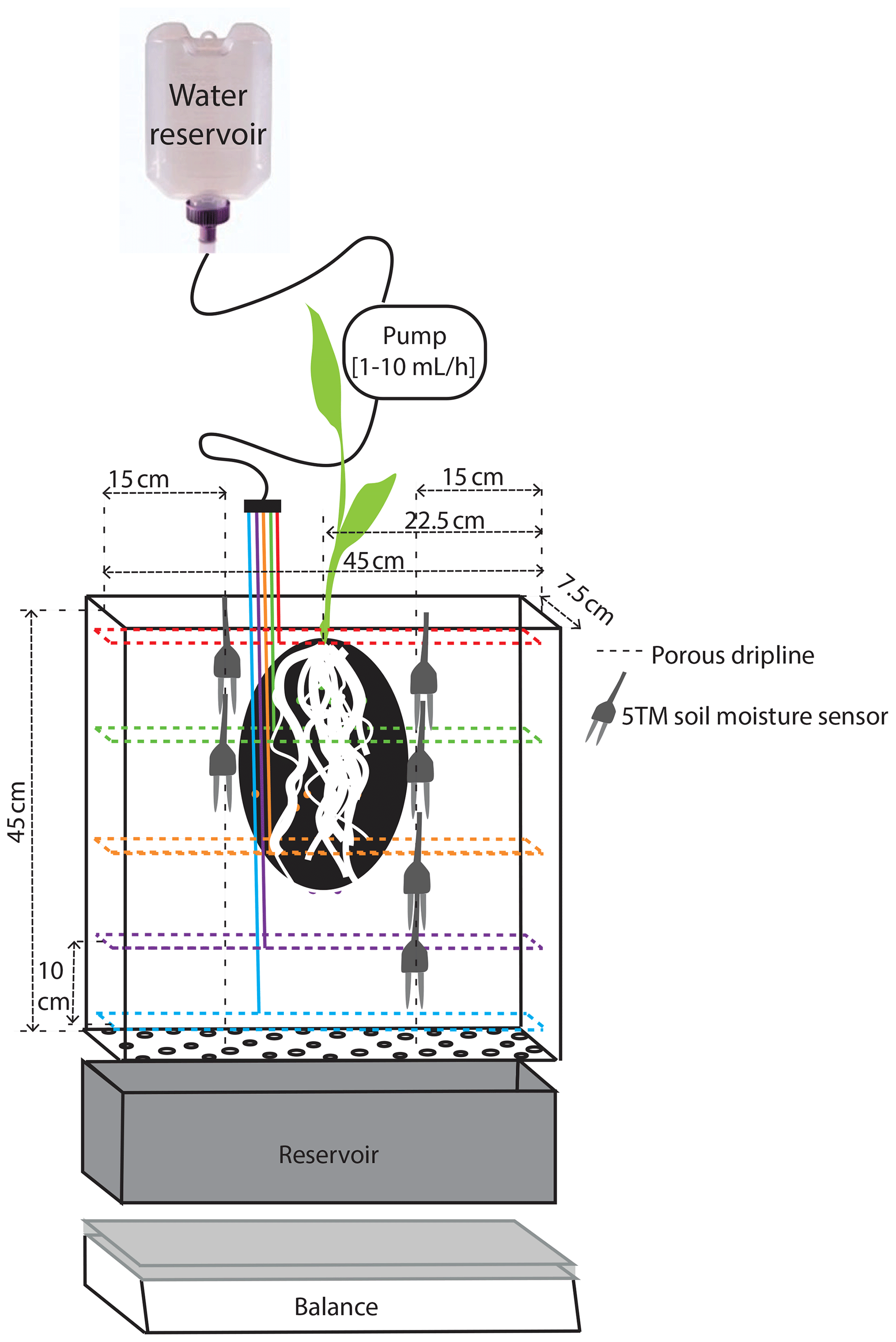
Figure 1 Schematic representation of the experimental setup inside a rhizobox. The dashed colored lines represent the driplines at the different levels.

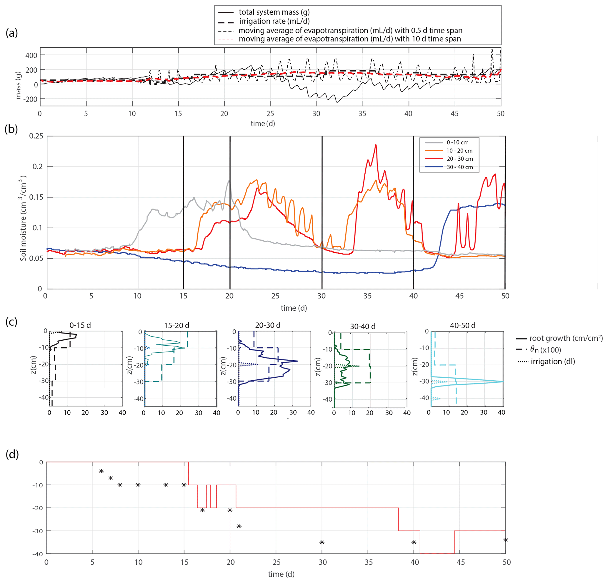
Figure 2 (a) Time series of the overall system mass, irrigation rate, and evapotranspiration. (b) Time series of the soil moisture within four different depth intervals. (c) Total root length that appears in the considered time frame (solid lines), time-averaged soil moisture profiles (dashed lines), and total applied irrigation volume (dotted lines). Root development is most pronounced in the intervals with the largest soil moisture. (d) Applied irrigation depth (red line) and observed maximum rooting depth (markers).

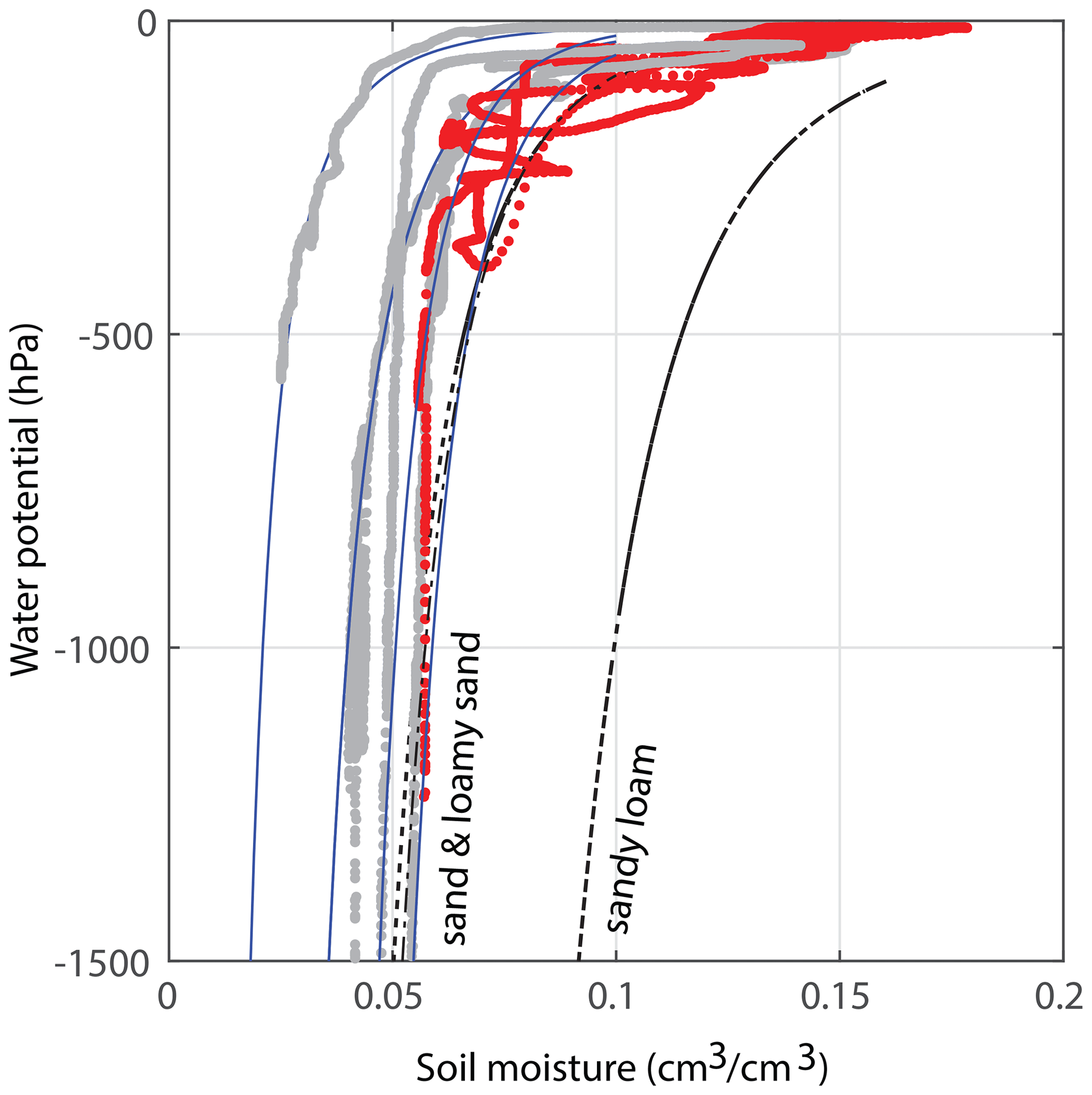
Figure 3 Estimates for the water retention curve of the applied soil. The red data have been obtained during the main experiment of this publication; at 30 cm depth, a water potential TEROS 21 sensor was installed about 15 cm away from the soil moisture sensor. This is a rough estimate, as the sensors are not (and cannot be) installed directly next to each other. The gray curves were derived from other experiments with the same sand : potting soil ratio. All blue lines are fits that fall within the theoretical variations for sand and loamy sand (i.e., within the standard deviations of these soil types, according to Clapp and Hornberger, 1978). The black curves are the curves for the average sand, loamy sand, and sandy loam. Note that the graphs of other soil types such as clay/clay–sand are very different and not visible on these axes.

2 Experiments

2.1 Experimental setup

We study 50 d of evolution of a maize soil–root system inside a rhizobox (with a length × width × height of 45 × 7.5 × 45 cm, respectively; see Fig. 1). Irrigation is supplied continuously at a low flow rate through porous driplines (with an inside diameter of 4 mm) that were installed at five different levels (with 10 cm intervals) at 1.5 cm distance and parallel to each window (see Fig. 1). The flow rate is constant throughout the day but adjusted in steps (in an attempt to follow the water demand of the plant; see the dashed black and red curves in Fig. 2a). To control the vertical soil moisture gradients, the irrigation depth was increased over time to moisten the deeper soil layers one by one (see Fig. 2d). Irrigation is applied to one depth at a time. The rhizobox was filled with a sifted black potting soil (Pokon universal potting soil, which is largely made up of peat moss) and sand mix (weight ratio 1:2.7; see Fig. 3 for the lab-determined water retention curve). The soil moisture is measured continuously at four depths inside the rhizobox with ECH20 EC-5 soil moisture sensors. Every few days the root growth is monitored by tracing the roots on a transparent sheet through the transparent window. Subsequently, pictures were made of the transparent sheets, and Fiji ImageJ software was used to measure root lengths and (a proxy for) root densities (i.e., the total measured root length in each vertical centimeter divided by the horizontal dimension of the rhizobox of 45 cm). At the bottom, a drainage reservoir was installed. The top of the soil was covered with plastic to prevent evaporation from the soil. The setup was placed on a 1 g precision scale (Mettler Toledo MS32000Le/01) to track the overall water balance. It should be noted, however, that the total time series of the system mass, as plotted in Fig. 2a, was subjected to multiple extrapolations from shorter time series (with time spans from hours to days) to deal with (daily) interruptions during the execution of the experiments. Furthermore, the increase in the plant mass was neglected. The aboveground wet biomass was measured after the whole period to be 105 g (determined by cutting the plant at ground level and measuring the corresponding weight change), which is small compared with the gross irrigation and evapotranspiration fluxes (typically about 100 g daily) but significant compared with the net changes in the water balance. The weight measurements were mainly used to have an estimate for the evapotranspiration flux, which is compared with the simulations, and to determine the long-term water demand or abundance in order to adjust the irrigation rate to what the plant needs. The experiment starts at t=0, when a maize plant (which was sown around 2 weeks earlier in a small pot) with a maximum root length of 5 cm and an aboveground height of 10–15 cm was placed inside the rhizobox.

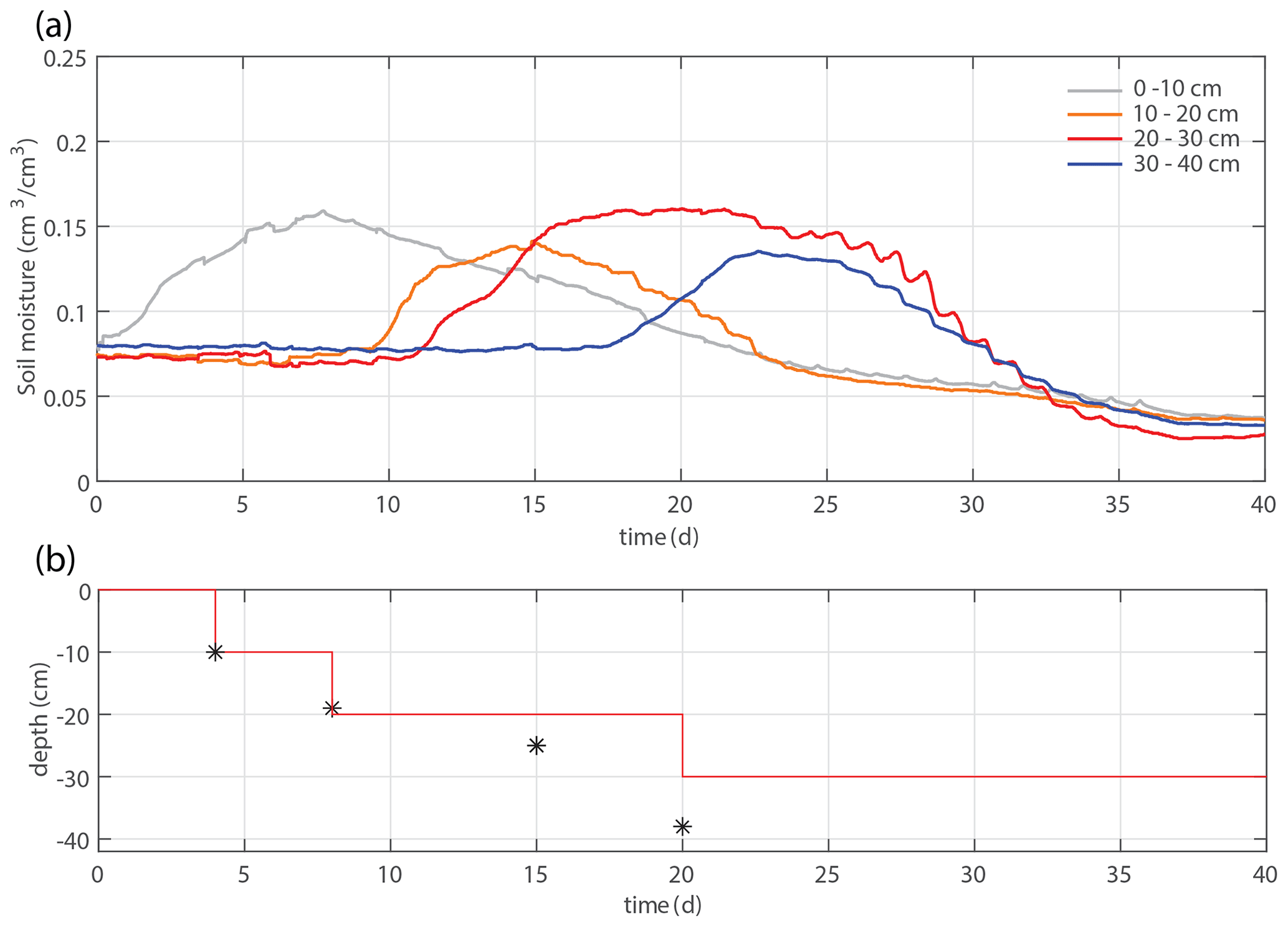
Figure 4 (a) Time series of the soil moisture within four different depth intervals. (b) Applied irrigation depth (red line) and observed maximum rooting depth (markers).

2.2 Diagnostic model of root growth: root follows moisture

2.2.1 Time series and correlations

Figures 2 and 4 show two experiments with a varying irrigation strategy that were used for further model formulation and model validation, respectively. Qualitative results of a third experiment with yet another different irrigation strategy can be found in the Supplement. For the main experiment, the soil moisture development is plotted together with profiles of the soil moisture and root density growth within succeeding periods in Fig. 2b–c. Root development is found to be most pronounced at depth intervals with the highest soil moisture. These results suggest that soil moisture and root growth distributions are strongly connected.

2.2.2 Model formulation

As a first step to model the flexible root growth, we test the following (straightforward) diagnostic equation to calculate the root growth rate distribution as function of the (normalized) soil moisture:

$$\begin{array}{}\text{(1)}& {\displaystyle \frac{\partial R}{\partial t}}{\displaystyle \frac{\mathrm{1}}{r}}={\displaystyle \frac{{\mathit{\theta }}_{\mathrm{n}}}{{\int }_L^{\mathrm{0}}{\mathit{\theta }}_{\mathrm{n}}\mathrm{d}z}},\end{array}$$

where R(z,t) (cm cm⁻³) is the root density profile, θ_n is the normalized water content, and

$$\begin{array}{}\text{(2)}& {\mathit{\theta }}_{\mathrm{n}}={\displaystyle \frac{\mathit{\theta }-{\mathit{\theta }}_{\mathrm{w}}}{{\mathit{\theta }}_{\mathrm{s}}-{\mathit{\theta }}_{\mathrm{w}}}},\end{array}$$

with θ_s as the saturated water content and θ_w the wilting point; i.e., the minimum amount of water in the soil that is required for any water absorbance by the roots (Kirkham, 2005).

r(t) in Eq. (1) is the depth-integrated root growth,

$$\begin{array}{}\text{(3)}& r\left(t\right)=\underset{L}{\overset{\mathrm{0}}{\int }}{\displaystyle \frac{\partial R}{\partial t}}\mathrm{d}z,\end{array}$$

with L(t) (cm) as the maximum vertical rooting depth, which is assumed to increase linearly in time by a constant growth rate u₁, as follows:

$$\begin{array}{}\text{(4)}& {\displaystyle \frac{\partial L}{\partial t}}=u_{\mathrm{1}}.\end{array}$$

Hence, Eq. (1) links the local root growth tendency, normalized by the bulk growth tendency, to the local soil moisture, which is also normalized by the bulk soil moisture. In other words, the hypothesis is that the vertical root growth distribution linearly follows the vertical soil moisture distribution.

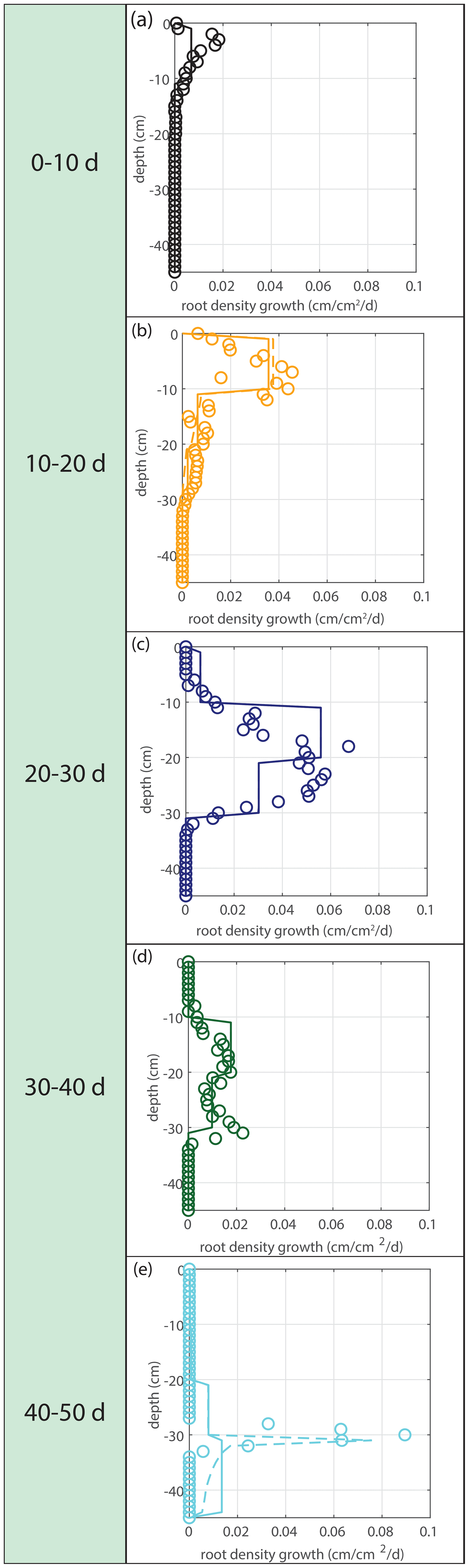
Figure 5 Vertical profiles of averaged root growth rates within succeeding periods as observed (circles) and as diagnostically calculated by Eq. (1) (roots follow moisture principle; solid lines), using the measured bulk root growth and soil moisture profiles. Dashed lines are simulations with a threshold for root growth (θ > 0.075).

Figure 6 Sensitivity of root growth profiles to different values of the vertical root growth rate u₁. The different colors refer to the consecutive time periods of Fig. 5; i.e., the graphs represent 10 d averages of the daily root density growth rates.

2.2.3 Model parameter evaluation and results

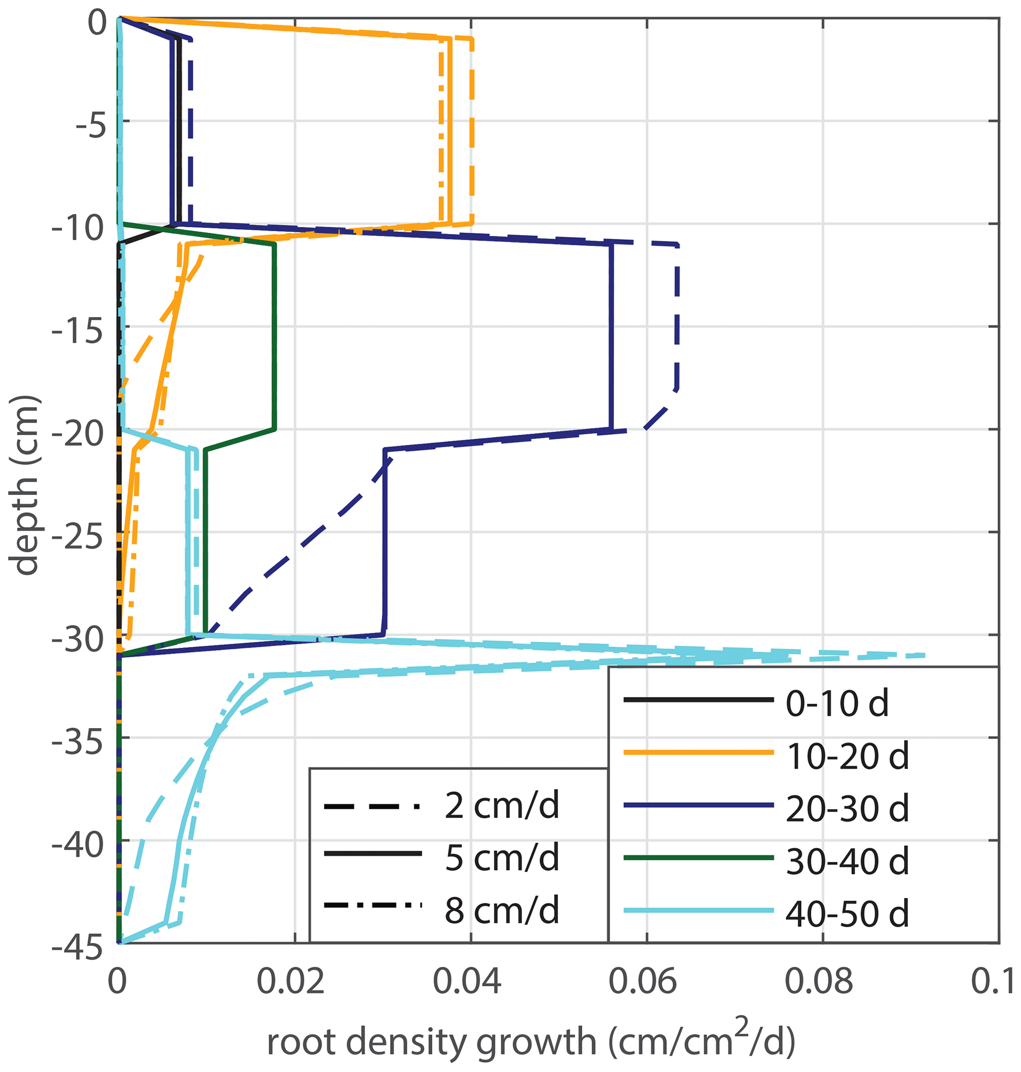
Modeled root growth profiles are compared with the experimental data for successive time periods (see Fig. 5a–e). Note that the two-dimensional root length density observed at the window (in cm cm⁻²) is used as a direct proxy for the actual root length density R(z,t) (cm cm⁻³). For the results in Fig. 5 and for the further experiments presented in this paper, the extension rate of rooting depth is taken as u₁=5 cm d⁻¹ (based on model comparison with the observed root profiles). In Fig. 6, the sensitivity to this parameter is investigated. For the wilting point, we take θ_w=0.075 (Saxton and Rawls, 2006; Yost, 2016). Patterns of root growth are represented fairly well (Fig. 5), with the exception of the sharp local peak that occurs within the time slot 40–50 d (at $z=-\mathrm{30}$). This latter case is improved by adopting an extra condition for vertical root growth at the root tip, namely that no vertical root growth occurs if the soil moisture at the root tip is smaller than θ=0.075 (see Fig. 5).

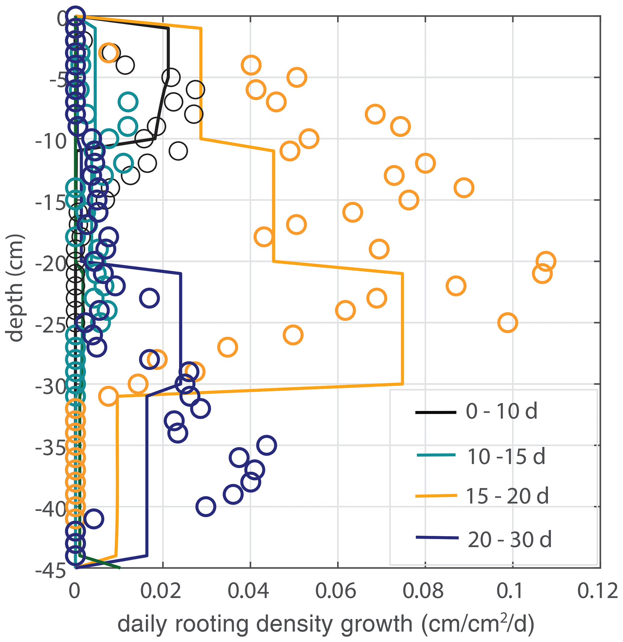
Figure 7 Model validation. Vertical profiles of modeled (lines) and observed (circles) root growth for the second data set with a different irrigation schedule and identical model parameter u₁ (and a threshold for root growth at the root tip of θ > 0.075, but the simulation is found to be insensitive to this parameter). No significant additional root growth was observed after 30 d.

2.2.4 Model validation

To validate the model and the evaluated parameters, we use a second experiment with an identical experimental setup but a different irrigation schedule. In contrast to the main experiment, the irrigation depth is adjusted directly when roots are observed at a new (deeper) irrigation level (the bottom layer was wetted by the dripline at the second-deepest level, however, so that the bottom line has not been used). The whole box was moistened within 25 d, and the observed maximum rooting depth develops faster. Time series of the soil moisture and irrigation depth are indicated in Fig. 4, while Fig. 7 shows a comparison of the measured root density profiles with the model, using the same parameter value of u₁=5 cm d⁻¹. No significant additional root growth was observed after 30 d.

2.3 Soil moisture and water uptake model

2.3.1 Model formulation

Soil moisture and root growth are interacting variables. To gain insight into the interaction between both variables, we aim to simulate the time evolution of both variables prognostically. We therefore also need a formulation for how roots in turn affect soil moisture.

To calculate the evolution of the water content (θ) due to irrigation, soil water flow, and plant water uptake, we the apply the Richards equation, as follows:

$$\begin{array}{}\text{(5)}& {\displaystyle \frac{\partial \mathit{\theta }}{\partial t}}={\displaystyle \frac{\partial q}{\partial z}}-S+I,\end{array}$$

with S (cm³ cm⁻³ min⁻¹) as the soil water extraction by plant roots, I (cm³ cm⁻³ min⁻¹) as the irrigation, z (cm) as the vertical coordinate taken positively upward, and q (cm min⁻¹) as the soil water flux density (positive upward). q is given by Darcy's equation, as follows:

$$\begin{array}{}\text{(6)}& q=K\left(h\right){\displaystyle \frac{\partial (h+z)}{\partial z}},\end{array}$$

with K (cm min⁻¹) as the hydraulic conductivity and h (cm) as the soil water pressure head. Following (Clapp and Hornberger, 1978), h is taken as

$$\begin{array}{}\text{(7)}& h=h_s{\left({\displaystyle \frac{\mathit{\theta }}{{\mathit{\theta }}_{\mathrm{s}}}}\right)}^{-b},\end{array}$$

and K is taken as

$$\begin{array}{}\text{(8)}& K=k_{\mathrm{s}}{\left({\displaystyle \frac{\mathit{\theta }}{{\mathit{\theta }}_{\mathrm{s}}}}\right)}^{\mathrm{2}b+\mathrm{3}},\end{array}$$

with h_s and k_s, respectively, being the soil water pressure head (cm) and conductivity at saturation, θ_s is the saturated water content, and b is an empirical exponent. The values of k_s, θ_s, and b are taken from Clapp and Hornberger (1978) and correspond to loamy sand.

Following Adiku et al. (1996), the soil water extraction S is calculated by

$$\begin{array}{}\text{(9)}& S=u_{\mathrm{2}}R{\mathit{\theta }}_{\mathrm{n}},\end{array}$$

where u₂ is the water extraction rate per centimeter of root in saturated conditions (mL cm⁻¹ min⁻¹ or cm³ cm⁻¹ min⁻¹), S is the actual soil water extraction by plant roots per soil volume per minute (mL cm⁻³ min⁻¹), and R(z,t) is the root length density, i.e., roots per soil volume (cm cm⁻³).

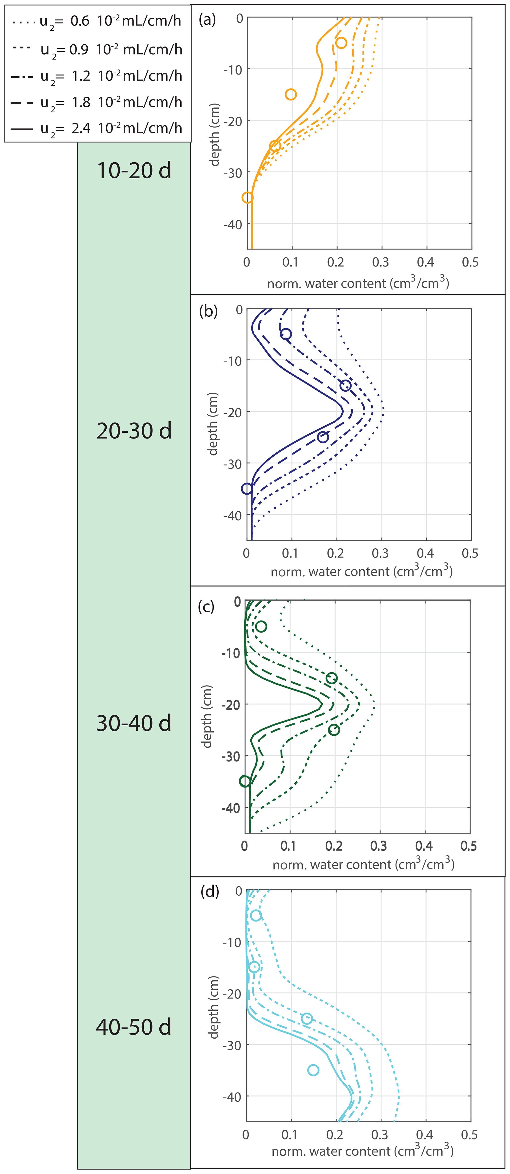
Figure 8 Sensitivity analysis for the water extraction rate per centimeter of root in saturated conditions u₂.

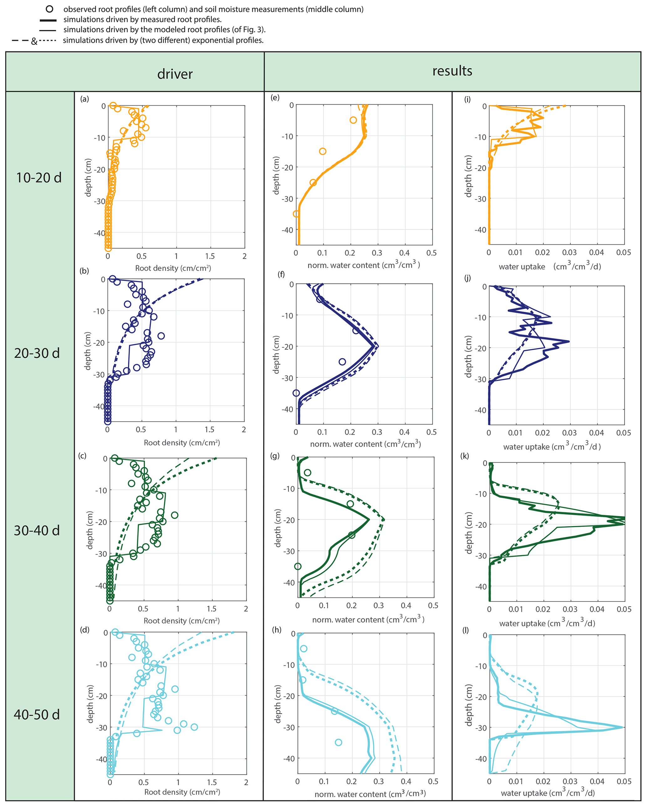
Figure 9 Offline simulations of time-averaged soil moisture (middle column) and water uptake (right column) for the measured root profiles at the start of each period for the calculated root profiles and for exponential equivalents.

2.3.2 Model parameter evaluation

The water extraction rate per centimeter of roots in saturated conditions u₂ is determined by comparing the soil moisture data with the soil moisture simulations driven by the measured root density data. The sensitivity to a range of tested variations is indicated in Fig. 8. The first 10 d were omitted because of the lack of observable root growth; it took a couple of days before the roots could be observed at the window. For Fig. 9 and the further experiments, we take $u_{\mathrm{2}}=\mathrm{1.2}\times {\mathrm{10}}^{-\mathrm{2}}$ mL cm⁻¹ h⁻¹, based on observation.

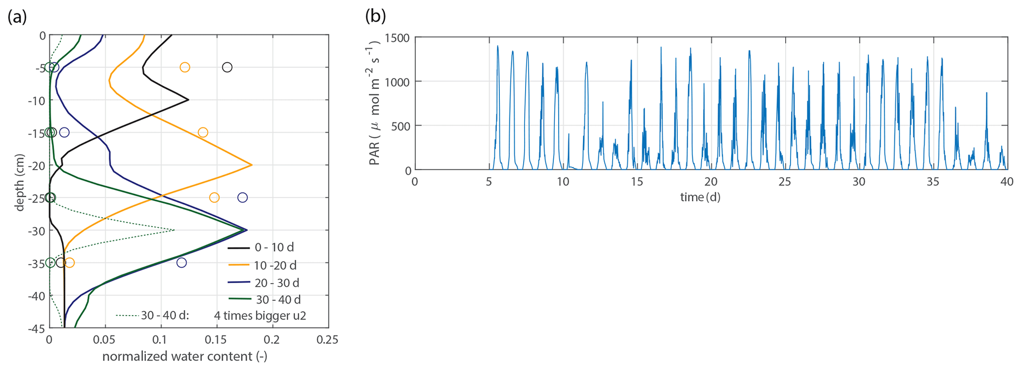
Figure 10 Model validation. (a) Vertical profiles of the normalized water content for the second data set, as described in Sect. 2.2.4, using the same parameter values (solid lines). For the period 30–40 d, an extra simulation is shown with a 4 times bigger value for u₂ ($\mathrm{4.8}\times {\mathrm{10}}^{-\mathrm{2}}$ mL cm⁻¹ h⁻¹). (b) Time series of the measured photosynthetically active radiation (PAR). A mature plant and higher PAR values are possible explanations for a greater water extraction rate per centimeter of root in saturated conditions.

2.3.3 Model validation

Figure 10 shows the modeled soil moisture profiles derived from the root profiles of the second data set by using the same parameter values (solid lines). For the period 30–40 d, an extra simulation is shown with a 4 times bigger value for u₂ ($\mathrm{4.8}\times {\mathrm{10}}^{-\mathrm{2}}$ mL cm⁻¹ h⁻¹), which is a better fit with the observations.

2.4 A prognostic model for coupled soil moisture and root growth

2.4.1 Model formulation

To prognostically simulate the time evolution of both variables, we implement the following equation for root density growth in the model described in Sect. 2.3:

$$\begin{array}{}\text{(10)}& {\displaystyle \frac{\partial R}{\partial t}}=u_{\mathrm{3}}{\mathit{\theta }}_{\mathrm{n}}.\end{array}$$

Hence, the local root growth tendency is now normalized by the (static) root density growth in optimal conditions (saturation) u₃ (cm cm⁻³ min⁻¹) instead of by the (measurable) bulk root growth tendency in Eq. (1). Equation (10) differs from the formulation proposed by Adiku et al. (1996), which includes a proportional dependency of the root growth on the local root length density. The simulations with the exponential equivalent are performed in a similar fashion. After each update of the root density profile, the exponential equivalent (with identical overall root length) is calculated and used for calculating the plant water uptake. The model is driven by irrigation data only.

2.4.2 Model parameter evaluation

The root density growth in saturated soil u₃ is estimated by comparing the simulated root profiles with the data. The sensitivity to the tested variations is indicated in Fig. 11. Based on the results in Fig. 11, we take u₃=0.2 cm cm⁻³ d⁻¹ for the simulations in Fig. 12.

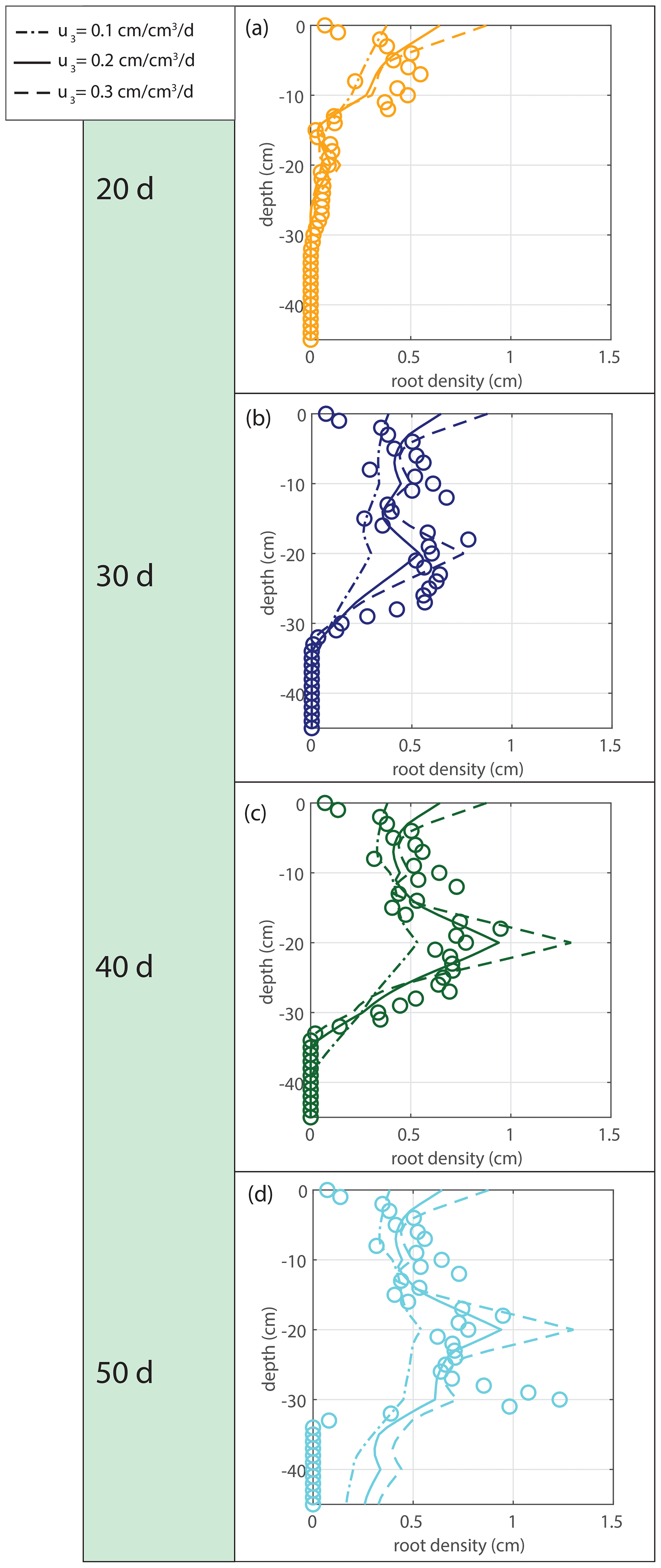
Figure 11 Sensitivity analysis for the root density growth rate in optimal (saturated) conditions u₃.

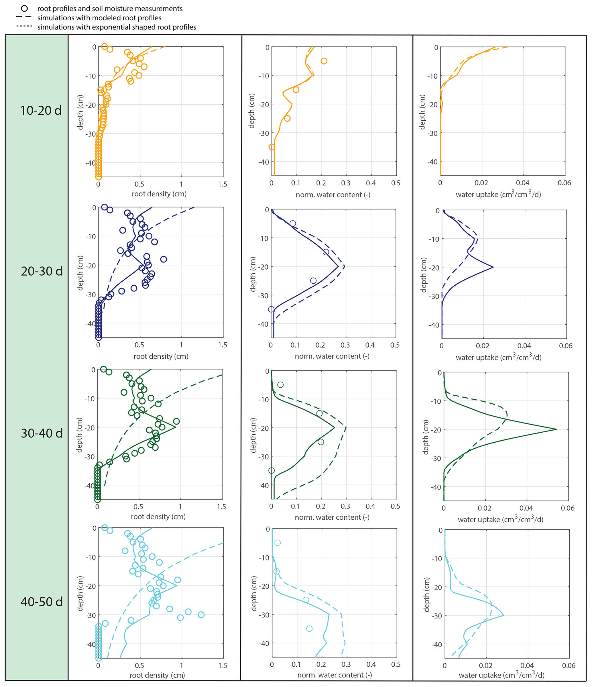
Figure 12 Fully coupled model with irrigation as the system driver. The left column shows the observed (circles), simulated (solid lines), and exponential (dashed lines) root profiles (at the start of each period). The middle column shows the corresponding soil moisture profiles. The right column shows the simulated uptake profiles for the simulated and exponentially shaped root profiles.

2.4.3 Model validation

Figure 13 shows the modeled soil moisture profiles derived from the root profiles of the second data set by using the same parameter values for u₁, u₂, and u₃. The model clearly underestimates root growth between days 10 and 20. The spatial patterns, however, are modeled reasonably well. In Fig. 14 a comparison is made between the results of different soils. The figure shows that the impact of the tested soil types (sandy loam versus loamy sand) is smaller than the impact of the tested u₂ values.

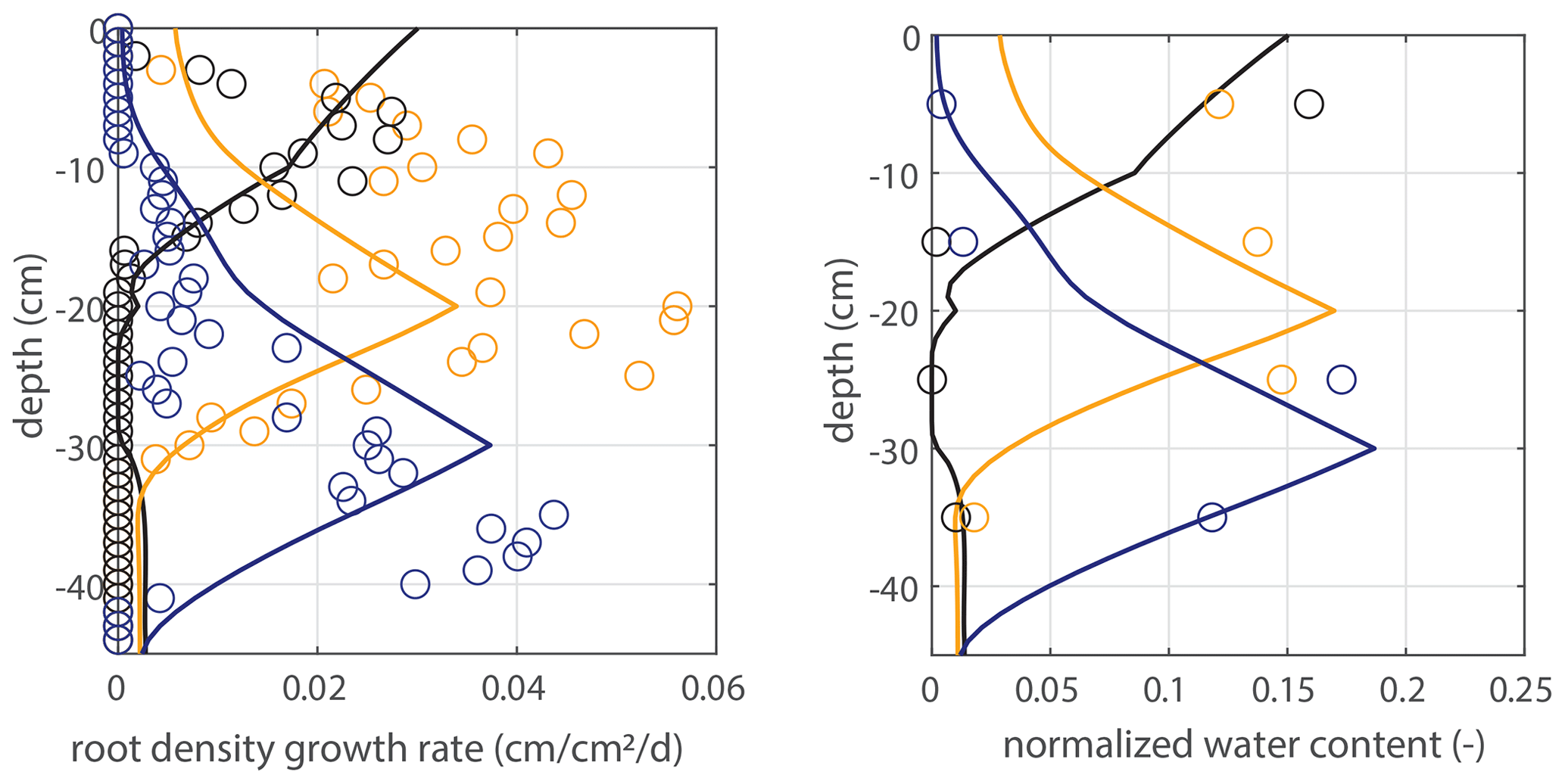
Figure 13 Model validation, with results for the second data set using identical model parameters.

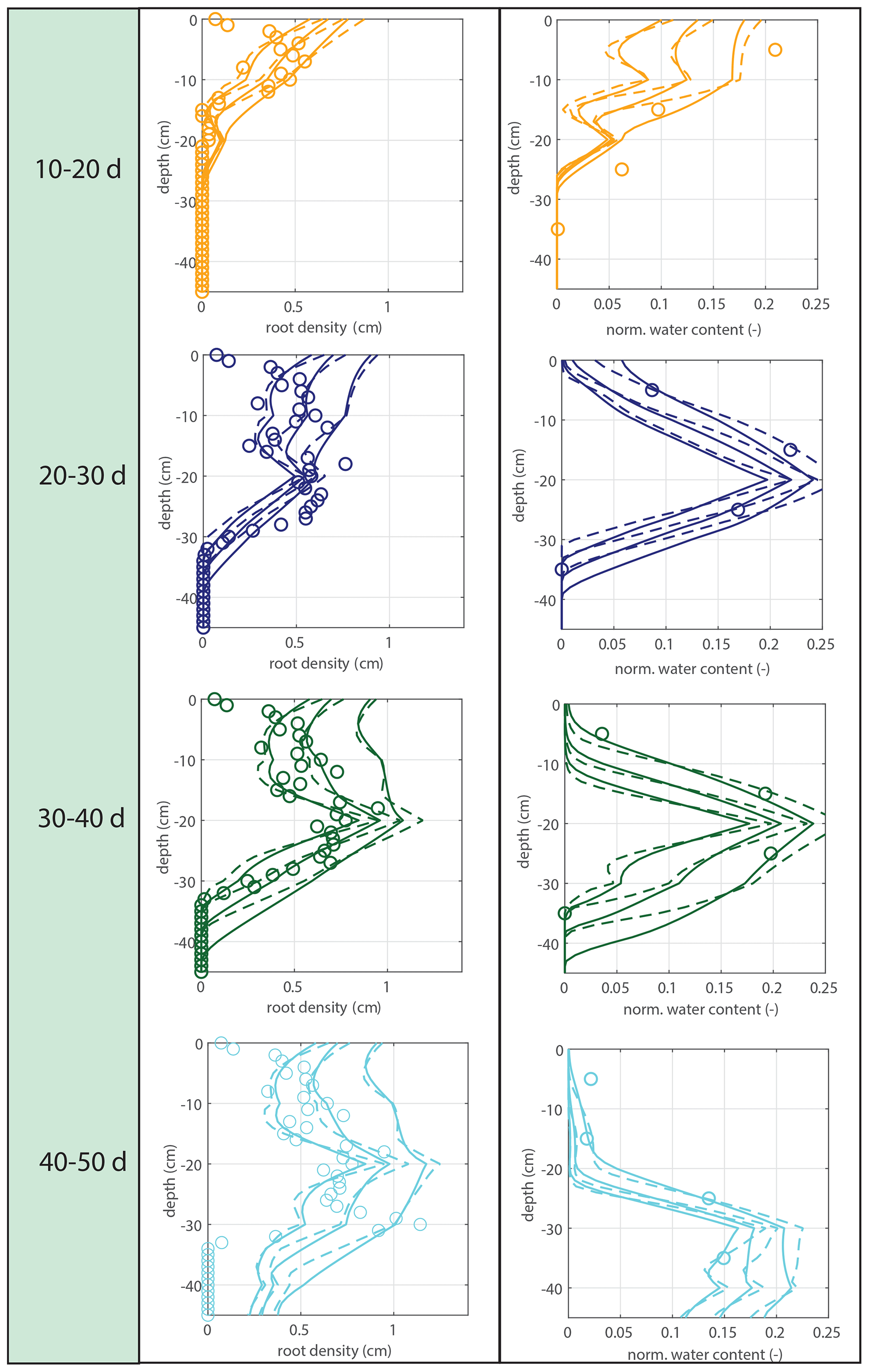
Figure 14 Comparison of results for loamy sand (solid lines) and sandy loam (dashed lines) for three different values for u₂ ($\mathrm{0.6}\times {\mathrm{10}}^{-\mathrm{2}}$, $\mathrm{1.2}\times {\mathrm{10}}^{-\mathrm{2}}$, and $\mathrm{2.4}\times {\mathrm{10}}^{-\mathrm{2}}$ mL cm⁻¹ h⁻¹).

3 Results and discussion

3.1 Diagnostic model

Figure 5 shows the observed and modeled root profiles. The observed root growth profiles deviate from simple exponential or linearly decreasing profiles. These patterns of root growth are represented fairly well by the model (Fig. 5).

Subsequently, soil moisture and water uptake rates were calculated for (1) the measured root profiles, (2) the calculated root profiles, and (3) for exponential equivalents (most roots in the upper soil), all with identical (measured) overall root growth rates. Figure 9 shows a comparison between those simulations and the observed soil moisture profiles. The soil moisture profiles derived from the modeled root profiles correspond fairly well with the soil moisture profiles derived from the measured root profiles (comparison solid and dashed lines in Fig. 9), whereas the results derived from the exponentially shaped root profiles show larger deviations, especially for the periods of 30–40 and 40–50 d. Furthermore, the simulations driven by the measured and modeled root profiles tend to correspond better with the measured total uptake rates compared to the simulations driven with the exponentially shaped root profiles (see Table 1). It has to be noted, however, that the derivation of the total water uptake rates show substantial uncertainties when considering the differences between the values derived from the mass balance and those derived from the observed soil moisture profiles (note that matching measurements would result in a value of 1 in the first column of Table 1). The differences between the simulations of the water components obtained with the different root profiles are relatively small compared to the large differences in the root profiles themselves. Even with the less realistic exponential root profiles, quite similar soil moisture profiles are found (Fig. 9). In each panel, the local peaks in the soil moisture coincide with the depths of irrigation. Smaller local root densities at these depths correspond with higher and wider soil moisture peaks (compare the dashed and dotted lines with the solid lines in the middle column of Fig. 9), which can simply be explained by the smaller local uptake rates. Note that wider peaks result, in turn, in a larger area in which uptake by plant roots can occur. Hence, this positive effect on the water uptake rates implies a negative (regulating) feedback loop between these components of the water balance (i.e., higher soil moisture leads to more water uptake, which subsequently reduces soil moisture), thus keeping the differences limited.

Table 1 Ratios of the calculated bulk water uptake rates (i.e., vertically integrated) to the measured bulk water uptake rates (derived from the mass balance). Calculations of the bulk water uptake are based on measured, modeled, or exponential root profiles (RPs).

3.2 Prognostic model

Also in a coupled fashion, driven by irrigation data only, the modeled root profiles are clearly improvements on the exponential profiles (left column in Fig. 12), except for the first 20 d, during which the exponential profile seems to be a good approximation. Also, the simulated soil moisture profiles (comparison of the data points with the dashed and solid lines in the middle column of Fig. 12) and the overall water extraction rates (Table 2) are slightly improved, although (as also for the diagnostic model) these differences were smaller than expected when compared to the relatively big differences in the root density distributions. Table 3 indicates that the exponential profiles resulted in larger overall (bulk) root lengths when compared with the flexible profiles. Note that the bulk root growth rate depends linearly on the vertically integrated soil moisture field via Eq. (10). An off-shape profile that results in higher vertically integrated soil moisture values will therefore trigger extra root growth. Hence, from a water balance perspective, an inefficient (unrealistic) profile shape is compensated by extra root growth, which (in another way) points (again) to the relevance of including soil-moisture-dependent (bulk) root growth for realistic water balances. This is in contrast with the linear dependency of the overall root growth on the overall biomass growth (independently of soil moisture), which is often assumed in crop and land surface models.

Table 2 Ratios of the calculated bulk water uptake rates (i.e., vertically integrated) to the measured bulk water uptake rates (derived from the mass balance). Calculations of the bulk water uptake are based on simulations with the coupled model with flexible root profiles (RPs) or exponential root profiles.

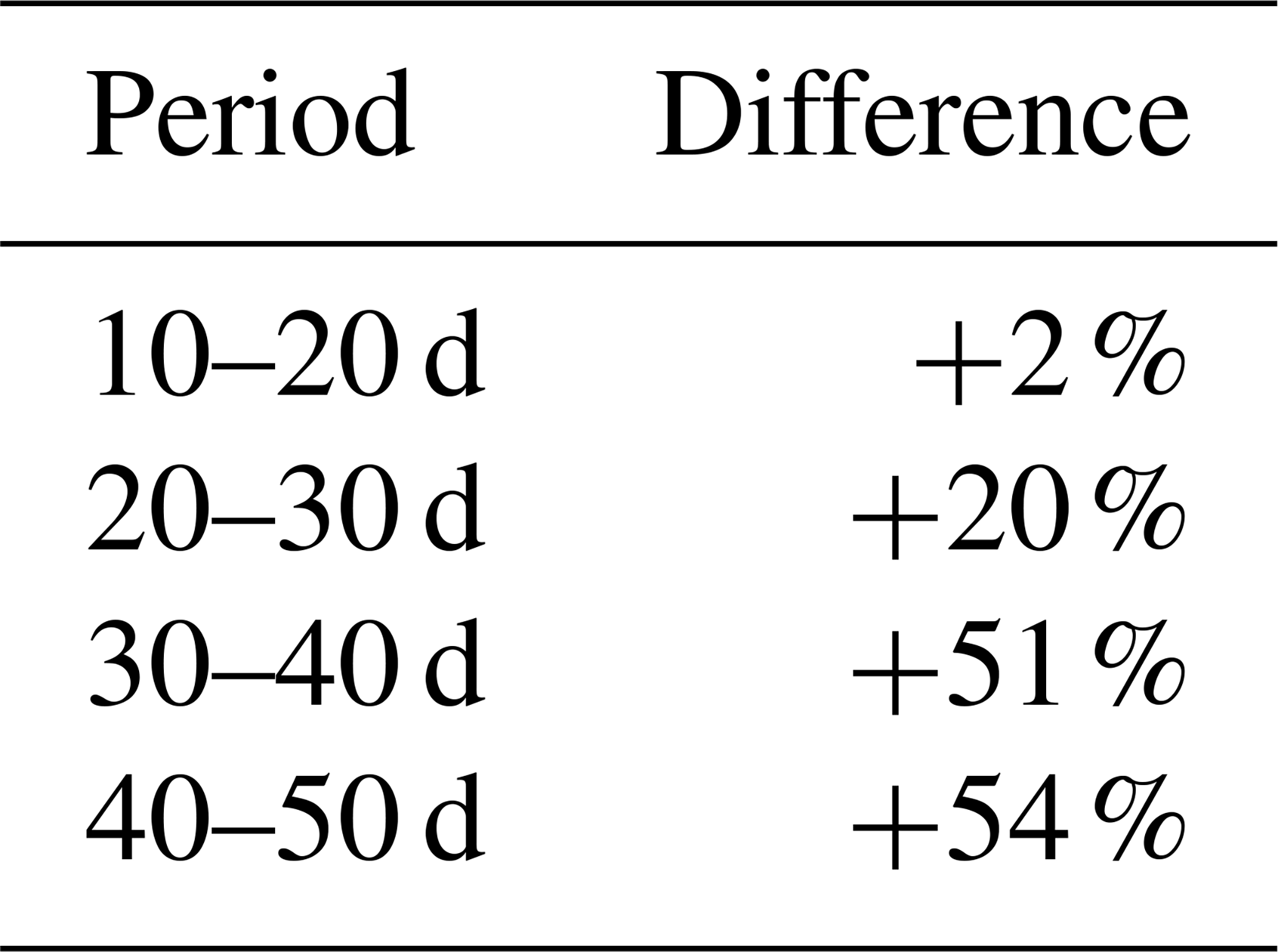
Table 3 Percentage increase in the total modeled root length in the case of exponential profiles instead of dynamic root profiles.

3.3 Applying the model at larger scales in crop and land surface models

We tested the model on single soil–plant systems. A next step is to consider its application at field scales and larger; i.e., to couple the routine for soil-moisture-dependent root growth to a crop or land surface model in order to link the model variables to measurables in the field. There are two options for applying the model in an existing land surface scheme, namely (1) applying Eq. (1) to include soil-moisture-dependent vertical root distributions (while using the standard procedure in the existing land surface scheme for calculating the bulk root growth) and (2) applying Eq. (10), i.e., soil-moisture-driven vertical distributions and bulk root growth. Hence, we do not advise including our water uptake routine. More advanced modules are already included in land surface models (and the water extraction rate per centimeter of root in saturated conditions is sensitive to aboveground settings, e.g., photosynthetically active radiation and potential evapotranspiration; see Fig. 10). We briefly discuss the field measurements that could be applied for parameter calibration and model validation here because the continuous measurement of root growth will be difficult at the field scale. Instead, one could derive and analyze sediment cores, including soil moisture and roots, on a spatial grid in the field at successive moments in time. Sensors for measuring soil moisture (profiles) can be applied in the field, and additionally, (satellite) remote sensing data can be used to derive (sub)surface soil moisture (subjected to an infiltration scheme) and evapotranspiration fluxes for parameter evaluation and model validation. Precipitation data will be needed for forcing the land surface model.

4 Conclusions

Our results confirm that there is a strong, and dominant, influence of soil moisture on root density growth and the extension rate of the maximum rooting depth. We show that root profiles can be predicted realistically from information on soil moisture profiles only. If soil-moisture-driven root growth is coupled to a vertical water transfer model, both the root and soil moisture profiles can be obtained based on water input, in addition to a few constants and simple principles. This suggests that root growth is mainly driven by soil moisture and is relatively insensitive to aboveground processes and overall biomass growth. However, a detailed (crop-specific) parameter study is needed for further validation and for generalizing the results based on a single soil–plant system.

Our results also suggest that, in our modeled soil–plant system, the effect of unrealistic root profiles on the water balance component is partly compensated by, for example, the spatial diffusion and soil-pressure-driven water flow redistribution. This means that missing information on the precise root distribution does not automatically mean that large errors in the water budgets are made. However, in the latter case, the correct water budget results from compensating errors rather than from the correct process mechanism.

This study treats root growth independent of aboveground processes, while such a dependence is plausible. However, our results suggest that the soil moisture status is a dominant factor influencing root growth. An underestimation of the impact of soil moisture on root growth rates can result in underestimated plant resilience to drought and environmental changes. Regarding the resilience to drought stress, we suggest that continuous, adequate root growth during periods of favorable soil moisture conditions might be a strategy for plants to prevent water stress during dry periods.

The conceptual simplicity of our proposed model enables straightforward implementation in regional land–atmosphere models that can replace current exponential root profiles. The main benefits will be a more correct representation of soil–plant water fluxes, especially in situations where soil moisture availability is predominant in the deeper soil layers.