Study on a mother wavelet optimization framework based on change-point detection of hydrological time series

Hydrological time series (HTS) are the key basis of water conservancy project planning and construction. However, under the influence of climate change, human activities and other factors, the consistency of HTS has been destroyed and cannot meet the requirements of mathematical statistics. Series division and wavelet transform are effective methods to reuse and analyse HTS. However, they are limited by the change-point detection and mother wavelet (MWT) selection and are difficult to apply and promote in practice. To address these issues, we constructed a potential change-point set based on a cumulative anomaly method, the Mann–Kendall test and wavelet change-point detection. Then, the degree of change before and after the potential change point was calculated with the Kolmogorov–Smirnov test, and the change-point detection criteria were proposed. Finally, the optimization framework was proposed according to the detection accuracy of MWT, and continuous wavelet transform was used to analyse HTS evolution. We used Pingshan station and Yichang station on the Yangtze River as study cases. The results show that (1) change-point detection criteria can quickly locate potential change points, determine the change trajectory and complete the division of HTS and that (2) MWT optimal framework can select the MWT that conforms to HTS characteristics and ensure the accuracy and uniqueness of the transformation. This study analyses the HTS evolution and provides a better basis for hydrological and hydraulic calculation, which will improve design flood estimation and operation scheme preparation.

1 Introduction

Under multiple influences of human activities, atmospheric circulation and other factors, the original evolution of river runoff is featured by randomness, fuzziness, nonlinearity, non-stationarity and multi-timescale variation, which breaks the consistency in the “three properties” of hydrological time series (HTS; formed by the time arrangement of hydrological elements such as rainfall and runoff) (Chen et al., 2021; Fang and Shao, 2022). Independent and identically distributed (IID) is an assumption of mathematical statistics in hydrological and hydraulic calculation (Mat Jan et al., 2020). When the series cannot meet the IID, analysing its internal evolution and division will help to improve the accuracy and decision-making of the hydrological forecasting and operation scheme preparation by the mathematical model (Li et al., 2021).

In stochastic hydrology, HTS consist of deterministic components and stochastic components. The analysis of their evolution involves the period, trend and change point (Hobeichi et al., 2022). The period and trend mainly focus on deterministic components, while change-point detection is used to explain the stochastic components caused by various random and uncertain factors (Dang et al., 2021). Change-point detection determines the starting and ending points of period and trend division; thus it is the key to analysing HTS evolution (Şen, 2021). However, affected by feature uncertainty, change-point detection has become a complex problem because the extent, number and occurrence time of change points must be determined at the same time (Zhao et al., 2019). The t test, the two-sample Kolmogorov–Smirnov (K-S) test and the Shapiro–Wilk test are commonly used quantitative methods for series variation. In particular, the K-S test can calculate the degree of change by indicators such as asymptotic significance (two-tailed, p); therefore it is widely used (Jia et al., 2022).

Commonly used change-point detection methods include graphical methods (cumulative anomaly method, etc.), parametric methods (sliding t test and the Lee–Heghinian test, etc.) and nonparametric methods (ordered clustering method, Mann–Kendall test, and wavelet change-point detection, etc.). Graphical methods have the advantages of simple calculation and intuitive results, but the detection accuracy is low. Parametric methods assume that the series to be analysed obey a known distribution, which have certain limitations (Liu et al., 2022). Nonparametric methods have higher detection accuracy but are easily affected by factors such as parameter settings and series marginal effects (Stasolla and Neyt, 2019). Malki et al. (2022) used machine learning to compare the gap between historical data and forecasts from real-time monitoring data to determine whether the consistency of IoT energy consumption data has changed. Shi et al. (2022) constructed a single change-point test based on the covariance, cumulative sum and likelihood ratio of forecast residuals to detect the potential change point in time series. Corradin et al. (2022) constructed a Bayesian nonparametric multivariate change-point detection method by combining prior distributions with multivariate kernels and argued that the posterior probability of most change points should be lower than the posterior estimate. Xie et al. (2022) calculated the fitted local trend line based on the piecewise linear representation algorithm and the Akaike information criterion to realize change-point detection and series division and classified change points into three categories with the help of the slope and intercept. Change-point detection is of great significance to series division and is the basis for making full use of HTS to carry out more research. It can be seen that there is no unified standard to determine the change point of HTS. Therefore, this is a field worthy of further study.

After the change-point detection, the period and trend of HTS can be further explored. These methods include a cumulative anomaly method, the Mann–Kendall (M-K) test, continuous wavelet transform (CWT) and mode decomposition (empirical or extreme point symmetric, etc.) (De Oliveira-Júnior et al., 2022; Qin et al., 2021). Among them, CWT has a relatively complete theoretical system, which can comprehensively analyse the evolution of HTS and reveal their localization characteristics in the time domain (time variation) and frequency domain (frequency and amplitude variation), so it has been widely used in hydrology (Zerouali et al., 2022). However, the analysis results of CWT highly depend on the selection of the mother wavelet (MWT). Moradi (2022) optimized MWT by comparing the similarity of cross-correlation function, signal-to-noise ratio and mean standard error between the denoised series and the original. Benhassine et al. (2021) determined the optimal MWT by comparing the minimum mean square error between the original image and the denoised. Strömbergsson et al. (2019) proposed and verified the validity of using the Shannon entropy of the wavelet coefficients as the index for selecting MWT. However, change-point detection has not been explored by scholars to optimize the MWT that conforms to the series characteristics.

To solve the above problems, we proposed the change-point detection criteria based on a cumulative anomaly method, the M-K test, wavelet change-point detection and the K-S test, which can detect the consistency of HTS and complete a reasonable division. Furthermore, based on the detection accuracy, a MWT optimal framework that conforms to series characteristics was proposed, and the evolution analysis was summarized by CWT. This work proposed, in a pioneering way, an efficient way to optimize the MWT based on variance and change-point detention. Using the optimal MWT in CWT is helpful in catching the HTS evolution accurately and fully mining its information, which provides a feasible way to use inconsistent measured data for hydrological and hydraulic calculations.

2 Methodology

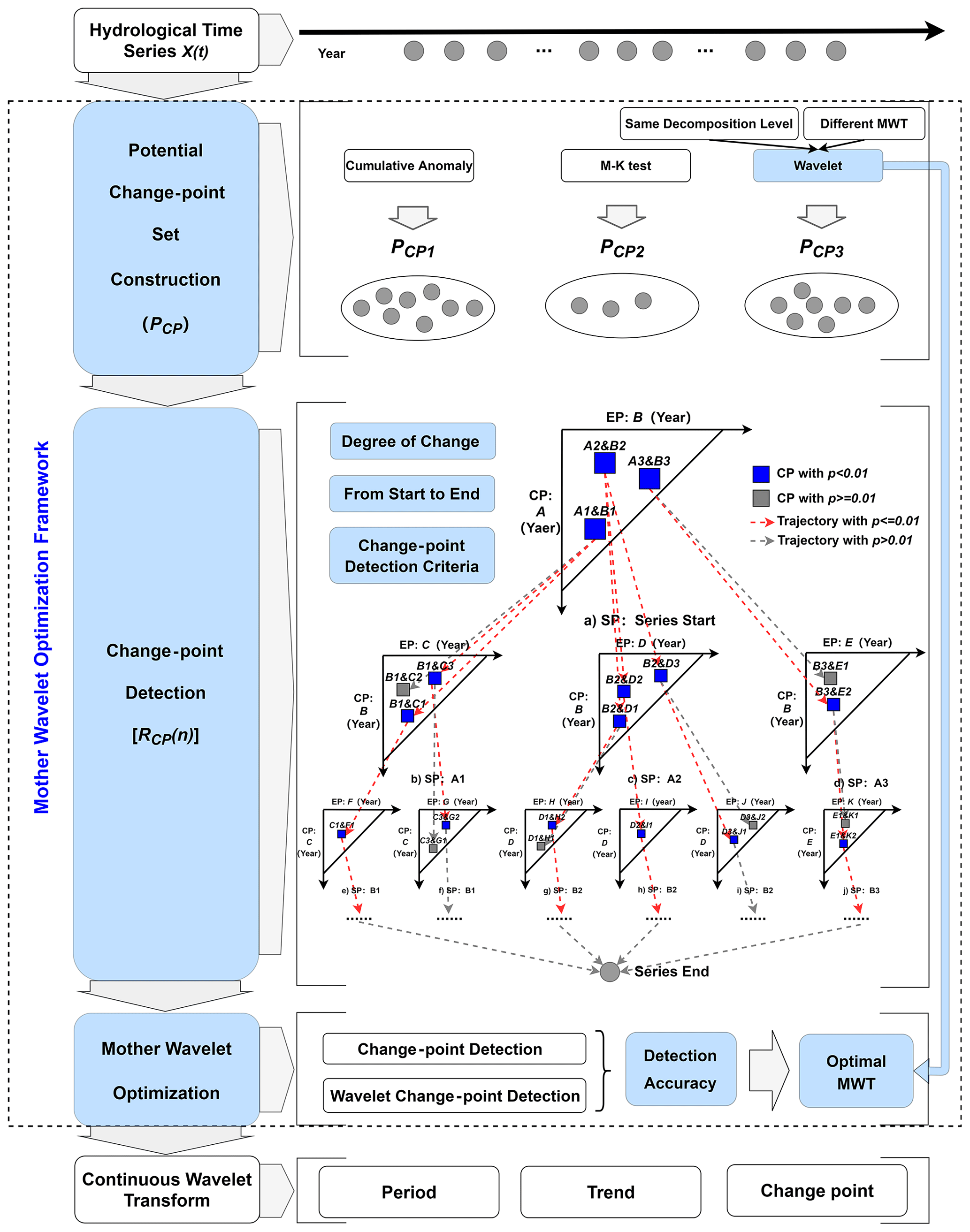
To solve the problems of incomplete change-point detection and non-unique MWT optimization, we followed the process of potential change-point set construction, change-point determination, MWT optimization and evolution analysis, and then we proposed the change-point detection criteria and the MWT optimization framework, as shown in Fig. 1.

Figure 1 Study framework and main modules of MWT optimization.

2.1 Wavelet transform and change-point detection

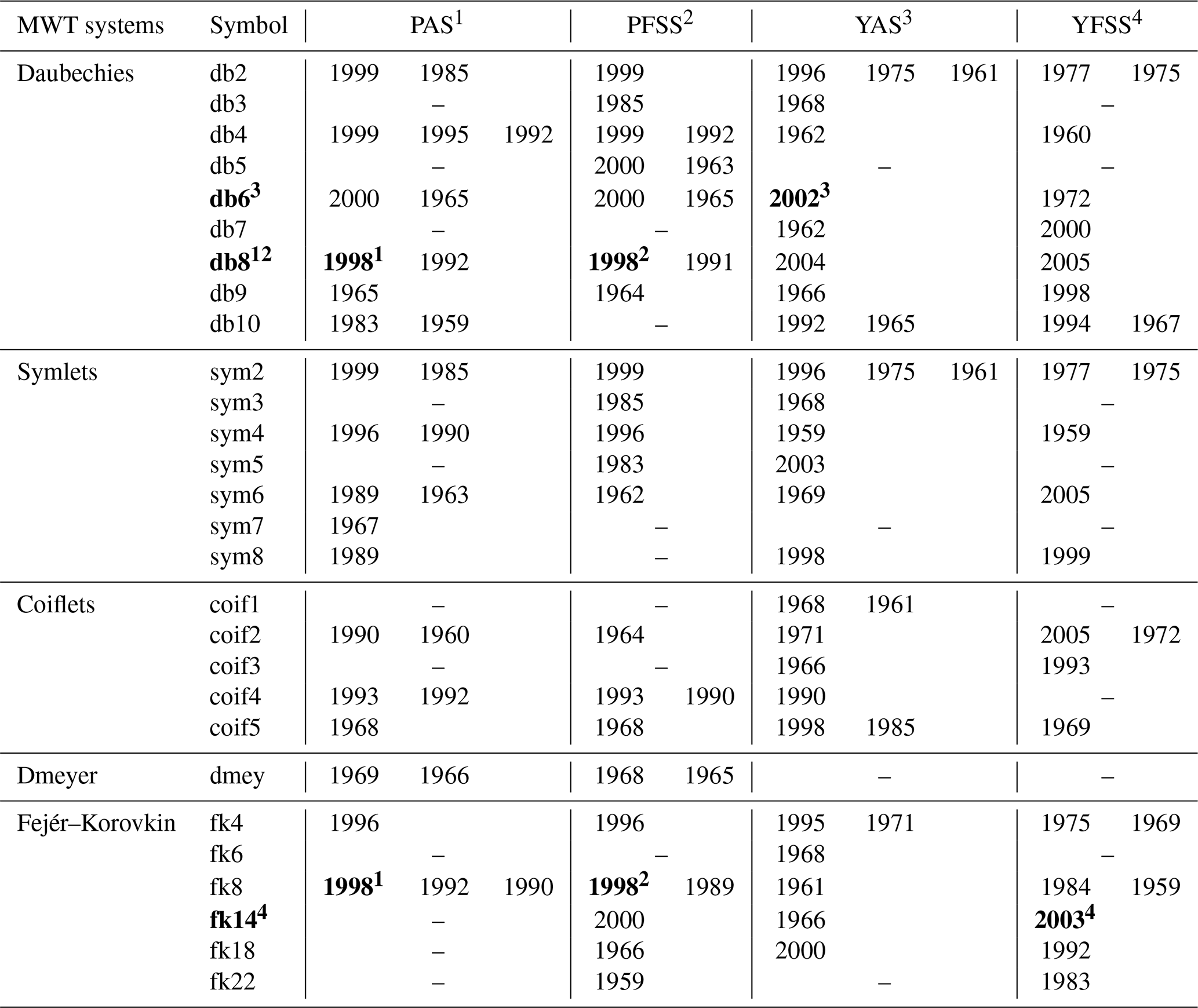
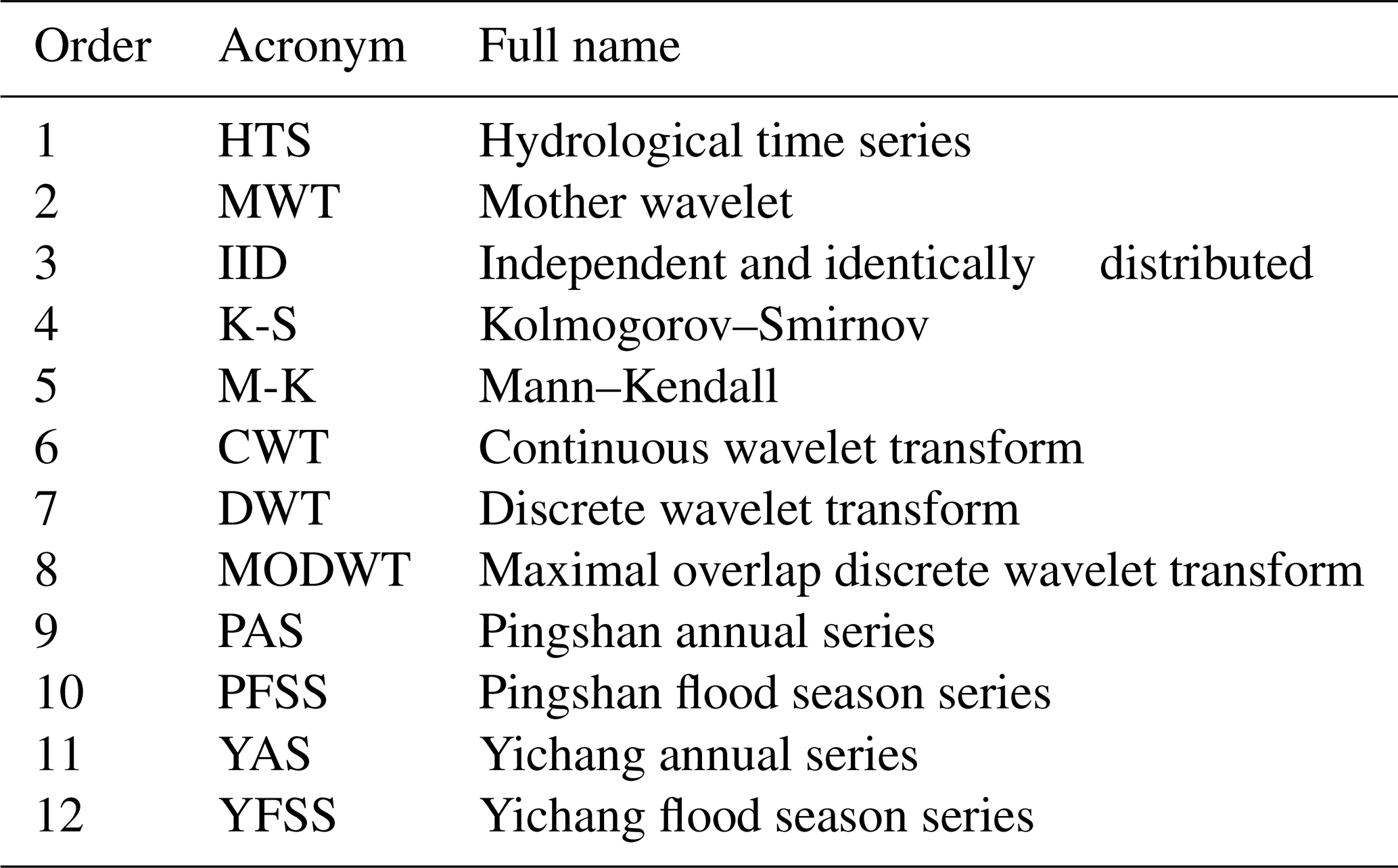
Wavelet transform can be divided into continuous wavelet transform (CWT) and discrete wavelet transform (DWT). Its essence is to reveal the similarity between the HTS to be analysed and the MWT. Therefore, the selection of MWT is a key factor affecting the accuracy of wavelet transform. MWT (φ(t)) is a wave of finite length and zero mean, with irregularity and asymmetry. The 16 commonly used MWT systems are shown in Table 1 (Moradi, 2022; Nielsen, 2001).

Table 1 Properties and application range of commonly used MWT systems.

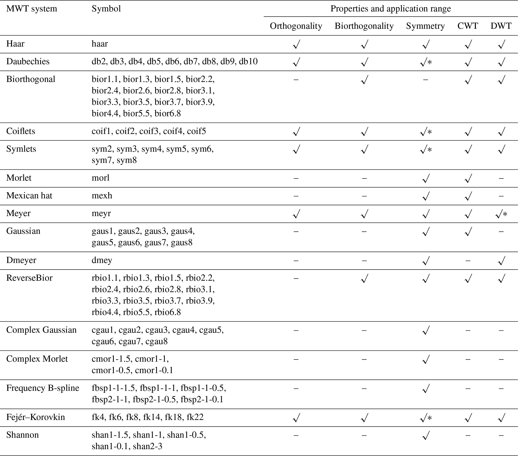
Note that “√” means has this property. “$\surd \ast$” means approximately having this property. “–” means does not have this property.

2.1.1 Continuous wavelet transform (CWT)

CWT can be used to determine whether there is periodicity in HTS and identify the main timescales and their local trends. Let L²(R) denote the measurable square-integrable functions on the real axis. If HTS X(t) ($t=\mathrm{1},\mathrm{2},\mathrm{\dots },T$) is a CWT in L²(R), which can be expressed as

$$\begin{array}{}\text{(1)}& {\displaystyle }{W}_X(a,b)=\underset{-\mathrm{\infty }}{\overset{+\mathrm{\infty }}{\int }}X\left(t\right){\mathit{\phi }}_{a,b}^{\ast }\left(t\right)\mathrm{d}t\text{(2)}& {\displaystyle }{\mathit{\phi }}_{a,b}\left(t\right)={\displaystyle \frac{\mathrm{1}}{\sqrt{a}}}\mathit{\phi }\left({\displaystyle \frac{t-b}{a}}\right)a,b\in R,a\ne \mathrm{0},\end{array}$$

where W_X(a,b) is the coefficient of CWT; ${\mathit{\phi }}_{a,b}^{\ast }\left(t\right)$ is the complex conjugate function of φ_a,b(t); t is the time; a is the timescale factor, which reflects the period length of MWT; and b is the time position factor, which reflects the translation of MWT in time.

The multi-timescale variation in wavelet transform refers to the multi-level structure and localized features of X(t) in the time domain, which is usually analysed with the help of the real part or modulus-square contour map of CWT coefficients. HTS evolution of a certain year on different timescales can be observed by vertically intercepting the contour map. At a certain period, the HTS evolution over time can be observed by horizontally intercepting the contour map. In addition, the positive wavelet coefficient corresponds to the wet season. The negative wavelet coefficient corresponds to the dry season. The wavelet coefficient is zero, which corresponds to the transition point of wet and dry. The larger the absolute value of the wavelet coefficient, the more obvious its change.

2.1.2 Discrete wavelet transform (DWT)

Since the measured HTS are usually discrete, by discretizing Eq. (1), we can get

$$\begin{array}{}\text{(3)}& {\displaystyle }{W}_X(j,b)=\underset{-\mathrm{\infty }}{\overset{+\mathrm{\infty }}{\int }}X\left(t\right){\mathit{\phi }}_{j,b}^{\ast }\left(t\right)\mathrm{d}t\text{(4)}& {\displaystyle }\mathit{\phi }{}_{j,b}\left(t\right)=a_{\mathrm{0}}^{\frac{-j}{\mathrm{2}}}\mathit{\phi }(a_{\mathrm{0}}^{-j}t-k{b}_{\mathrm{0}}),\end{array}$$

where W_X(j,b) is the coefficient of DWT, a₀ and b₀ are both constants, and j ($j=\mathrm{1},\mathrm{2},\mathrm{\dots },J$) is the decomposition level.

Both W_X(a,b) and W_X(j,b) are the values output by X(t) through the unit impulse response filter, which can reflect the evolution of X(t) in the time domain and frequency domain at the same time. In practical applications, it is often decomposed with the help of dyadic DWT, i.e. a₀=2 and b₀=1, and Eq. (4) can be expressed as

$$\begin{array}{}\text{(5)}& \mathit{\phi }{}_{j,b}\left(t\right)={\mathrm{2}}^{\frac{-j}{\mathrm{2}}}\mathit{\phi }({\mathrm{2}}^{-j}t-k).\end{array}$$

According to the dyadic DWT, the theoretical maximum value J of decomposition level j is

$$\begin{array}{}\text{(6)}& J=\left[{\log }_{\mathrm{2}}\right(T_{X\left(t\right)}\left)\right],\end{array}$$

where [⋅] represents the rounding operation, and T_X(t) represents the length of the X(t).

2.1.3 Wavelet change-point detection

Variance is one of the important parameters to detect whether HTS has fundamentally changed. Wavelet change-point detection is based on the maximal overlap discrete wavelet transform (MODWT). By calculating the variance of wavelet coefficients to be analysed one by one (Strömbergsson et al., 2019), the number and location of change point at a confidence level of 95 % can be determined through the MATLAB software toolbox.

(1) MODWT multi-resolution analysis

Decompose X(t) into T-dimensional column vectors $W_{\mathrm{1}},W_{\mathrm{2}},\mathrm{\dots },W_J$ and V_J, where W_J is calculated from the MODWT wavelet coefficient of X(t) within τ_jΔt, and V_J consists of τ_j+1Δt and higher dimensional MODWT scaling coefficients. X(t) can be expressed as

$$\begin{array}{}\text{(7)}& X=\sum _{j=\mathrm{1}}^J{D}_j+S_j,\end{array}$$

where $D_j=W_{j^{F^k}}^F{h}_j^{\ast }$ ($k=\mathrm{0},\mathrm{1},\mathrm{\dots },T-\mathrm{1})$ is the jth maximal-overlap detail. $S_j=V_{j^{F^k}}^F{g}_j^{\ast }$ is the jth maximal-overlap smooth. h_j and g_j are the high-frequency filter and the low-frequency filter, respectively. F is a T×T dimensional matrix that cyclically shifts h_j by one unit.

(2) MODWT variance decomposition

After a series of decompositions are performed on the variance of X(t) part by part, on the premise that the wavelet coefficient is stable, it can be expressed as

$$\begin{array}{}\text{(8)}& \Vert X{\Vert }^{\mathrm{2}}=\sum _{j=\mathrm{1}}^J\Vert W_j{\Vert }^{\mathrm{2}}+\Vert V_j{\Vert }^{\mathrm{2}}.\end{array}$$

Based on the above decomposition, the evolution of wavelet coefficient variance of X(t) with time in different timescales can be obtained, and the point where the variance changes can be recorded as the change point. It is worth noting that the MWT used for change-point detection needs to be biorthogonal (see Table 1).

2.2 Traditional change-point detection method

Change point detection has always been a significant issue in hydrology. However, except for the deterministic runoff changes caused by human activities such as large-scale river regulation, reservoir construction or operation (seasonal and above regulation capacity), there exist many uncertain factors, such as whether there is a change point in HTS, how many change points exist and the specific occurrence time of each change point. Therefore, it is necessary to integrate multiple detection methods. The main methods used in this study are as follows.

2.2.1 Cumulative anomaly method

The cumulative anomaly method is a graphic method. The cumulative anomaly value of X(t) at a certain time can be expressed as

$$\begin{array}{}\text{(9)}& \text{JP}\left[X\right(t\left)\right]=\sum _{t=\mathrm{1}}^N\left[X\right(t)-\stackrel{\mathrm{‾}}{X}],\end{array}$$

where JP[⋅] is the cumulative anomaly value of X(t), and T and $\stackrel{\mathrm{‾}}{X}$ are the length and mean of X(t), respectively.

The cumulative anomaly curve can be obtained by drawing the cumulative anomaly value in chronological order. According to the curve fluctuation, the change trend and potential change point of HTS can be identified. If the cumulative anomaly value is greater than 0, it indicates that the HTS is in an up trend; otherwise, the HTS is in a downtrend. The point that changes the trend can be regarded as the potential change point.

2.2.2 Mann–Kendall (M-K) test

The M-K test analyses the number, location, trend and significance of change points in HTS by setting a confidence level α and calculating statistics ($U_{F_k}$ and $U_{B_k}$). The $U_{F_k}$ statistics of X(t) is calculated as follows:

$$\begin{array}{}\text{(10)}& U_{F_k}\left[X\right(t\left)\right]={\displaystyle \frac{S_k^{X\left(t\right)}-E\left[S_k^{X\left(t\right)}\right]}{\sqrt{\text{Var}\left[S_k^{X\left(t\right)}\right]}}},\end{array}$$

where $U_{F_k}\left[X\right(t\left)\right]$ is the statistical series of X(t) calculated in order, and $S_k^{X\left(t\right)}$ is the rank sum of time k in X(t), which is the cumulative value of the numbers at time k greater than time i ($\mathrm{1}\le k\le i$). $E\left[S_k^{X\left(t\right)}\right]$ and $\text{Var}\left[S_k^{X\left(t\right)}\right]$ are the mean and variance of $S_k^{X\left(t\right)}$, respectively.

When $U_{F_k}\left[X\right(t\left)\right]>\mathrm{0}$, X(t) shows an upward trend; on the contrary, it shows a downward trend. The statistic $U_{B_k}\left[X\right(t\left)\right]$ is obtained by repeating Eq. (10) in the reverse order. Draw $U_{F_k}\left[X\right(t\left)\right]$ and $U_{B_k}\left[X\right(t\left)\right]$ in the same figure. If the two statistics intersect within the confidence interval $U_{\mathrm{0.05}}=\pm \mathrm{1.96}$ (confidence level 95 %), the time corresponding to the intersection is the change point of X(t).

2.2.3 Kolmogorov–Smirnov (K-S) test

The K-S test can determine whether the distributions of the two series are the same according to the maximum vertical distance between the two empirical distributions. The empirical distribution of X(t) is

$$\begin{array}{}\text{(11)}& F_n\left[X\right(t\left)\right]={\displaystyle \frac{\mathrm{1}}{T}}\sum _{t=\mathrm{1}}^T{I}_{[-\mathrm{\infty },T]}^n\left[X\right(t\left)\right],\end{array}$$

where $I_{[-\mathrm{\infty },T]}^n\left[X\right(t\left)\right]$ is the indicator function of X(t).

The original hypothesis H₀ is as follows: F₁[X(t)]=F₂[X(t)]; that is, the empirical distribution of the two series is consistent. The alternative hypothesis H₁ is as follows: F₁[X(t)]≠F₂[X(t)]; that is, the empirical distribution is inconsistent. To quantify the difference between the empirical distributions, a maximum difference D is proposed, calculated as

$$\begin{array}{}\text{(12)}& D=\underset{-\mathrm{\infty }<X\left(t\right)<\mathrm{\infty }}{sup}\left|F_{\mathrm{1}}\right[X\left(t\right)]-F_{\mathrm{2}}[X\left(t\right)\left]\right|.\end{array}$$

D_T,α is used to represent the rejection domain when the series capacity is T at significant level α. When $D\ge D_{T,\mathit{\alpha }}$, reject H₀; otherwise, accept H₀. To further quantify the significance of the difference, p is introduced to concretize α. The value of α is usually 95 % or 99 %, and the corresponding p is 0.05 and 0.01. If p≤0.01, it indicates that the determination result is strong and H₀ should be rejected; that is, the two series obey different distributions and are not consistent. If $\mathrm{0.01}\le p\le \mathrm{0.05}$, the determination result is weak. In this case, p is considered to be marginal, and H₀ is usually rejected. If p>0.05, H₀ is acceptable.

2.3 Change-point detection criteria

Based on the change-point detection results of various methods, the potential change-point set P_CP(n) ($n=\mathrm{1},\mathrm{2},\mathrm{\dots },N$) of HTS is constructed with deduplication and sorting. To determine the change point, it is necessary to further calculate the degree of change (p) before and after potential change points with the help of the K-S test. At a confidence level of 99 %, first, record the starting point and ending point of X(t) as P_CP(0) and P_CP(N+1) respectively, and arrange the potential change-point set in chronological order. Secondly, take P_CP(0) as the starting point and P_CP(1) as the change point, and use K-S test to successively calculate the p of the end point from P_CP(2) to P_CP(N+1). Finally, the change point and its trajectory (connection of change points) of X(t) are determined according to the change-point detection criteria:

• Criterion 1. Before and after the change point of X(t), p<0.01.

• Criterion 2. The change point can realize the continuous division of X(t) from P_CP(0) to P_CP(N+1).

• Criterion 3. The trajectory contains the largest number ($m=\mathrm{1},\mathrm{2},\mathrm{\dots },M$) of change points.

• Criterion 4. The p of M−1 in the trajectory is the minimum value.

2.4 MWT optimization framework

By comparing R_CP(n) and the results of wavelet change-point detection, a MWT that conforms to HTS characteristics can be selected. The MWT optimization framework includes the construction of potential change-point set, change-point detection and optimal MWT determination. Among them, the potential change-point set is built to improve the efficiency of change-point detection, and the specific optimization steps are as follows:

• Optimization step (1). Select candidate wavelet with the highest change-point detection accuracy.

• Optimization step (2). When two or more candidate wavelets have the same detection accuracy, the MWT or the MWT system with the highest frequency in different statistic series (length, flow, etc.) of the same hydrological station is selected as the optimal one.

After optimization, we can perform CWT according to the MWT conforming to HTS characteristics and analyse its evolution. For DWT, HTS can be more accurately decomposed and reconstructed, providing a good basis for hydrological forecasting and reservoir operation scheme formulation.

3 Data and study area

The Yangtze River originates from the southwest of the Tanggula Mountains on the Qinghai–Tibet Plateau. Its main stream flows through central China from west to east, with a total length of about 6300 km, and the total catchment area is 1.8×10⁶ km², accounting for about 18.8 % of the total area of China. The main stream from Yibin to Yichang is called the upstream, with a length of about 4504 km and an area of about 1×10⁶ km². With the superposition and collection of upstream floods to the Yichang hydrological station (Yichang station), it tends to form a process of high peaks and large volumes (Wang et al., 2021). The Pingshan hydrological station (Pingshan station) on the Jinsha River controls about half of catchment area and one-third of the flood season average flow of Yichang station and is the basic source of upstream flooding. Therefore, exploring the runoff evolution at Pingshan station and Yichang station will help to scientifically arrange the watershed storage space to alleviate the frequent floods in flood seasons and water shortages in dry seasons in the middle and lower Yangtze River. The overview of the upper Yangtze River is shown in Fig. 2, and the hydrological parameters of the tow stations are shown in Table 2.

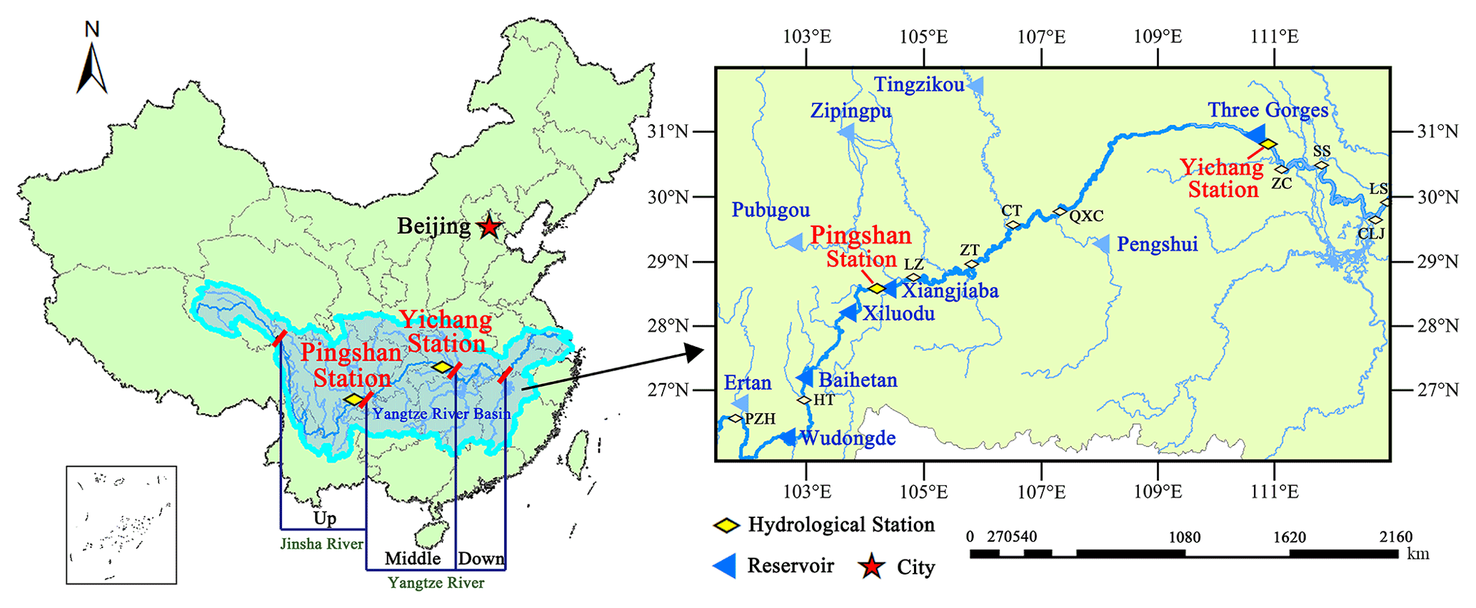
Figure 2 Location of the study area.

Table 2 Main hydrological parameters of Pingshan station and Yichang station.

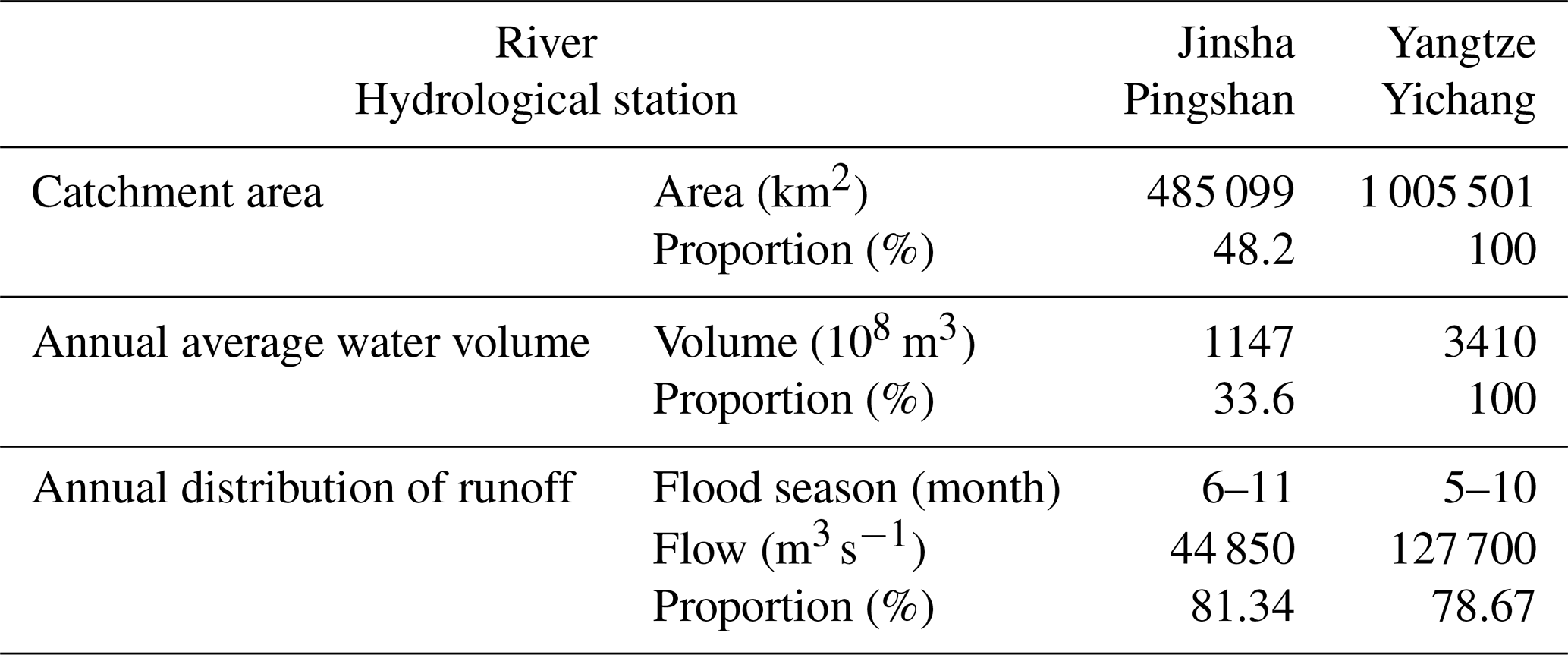
The flood season of Pingshan station is from June to November, and the flood season of Yichang station is from May to October. The three months with the largest flow on the two stations are both from July to September (accounting for 49.96 % and 54.18 % of the year, respectively). In 2012, Pingshan station was moved down 24 km to Xiangjiaba hydrological station. In addition, the runoff of Pingshan station should consider the influence of the upstream Ertan Reservoir (seasonal regulation, water storage in May 1998), and Yichang station should consider the Three Gorges Reservoir (annual regulation, water storage in June 2003). Combining the above factors, the measured runoff data of Pingshan station (1950–2011) and Yichang station (1950–2016) were used to test the applicability of the change-point detection framework and the MWT optimization framework proposed in this study, and the runoff evolution of the two stations was analysed by CWT.

4 Results and discussion

The statistical series of the two stations used in the study includes Pingshan annual mean runoff series (Pingshan annual series, PAS), Pingshan 6–11 mean runoff series (Pingshan flood season series, PFSS), Yichang annual mean runoff series (Yichang annual series, YAS) and Yichang 5–10 mean runoff series (Yichang flood season series, YFSS), collectively referred to as “4-Series”.

4.1 Construction of potential change-point set

The cumulative anomaly method, M-K test and wavelet change-point detection were used to detect the potential change points in the 4-Series. At the same time, by comparing the annual series and the flood season series at the same station, we further analysed the sensitivity of the three methods to the variation of flow amplitude and the influence of flood season on the annual series.

4.1.1 Results of cumulative anomaly method and M-K test

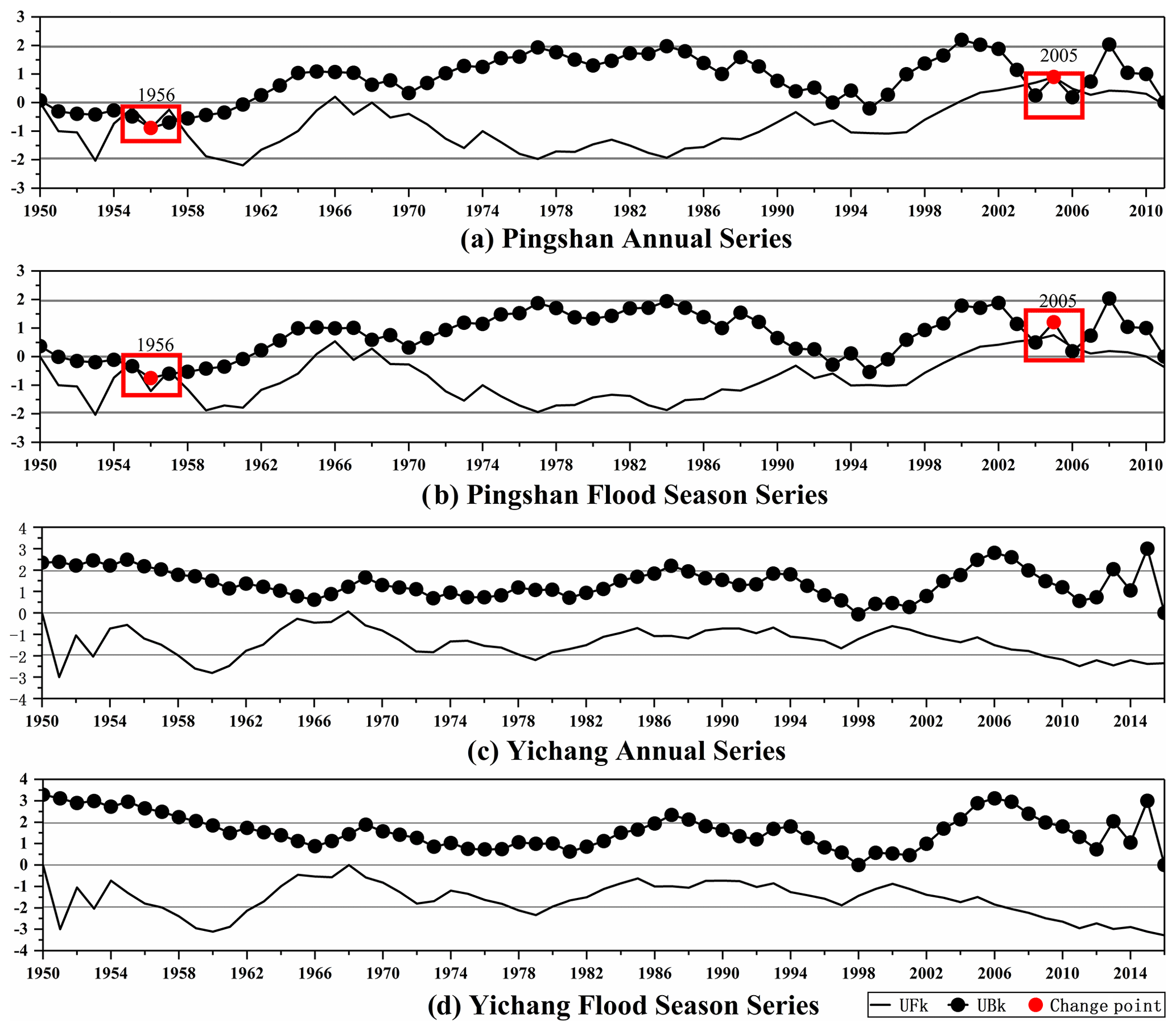
The points causing the trend change can be regarded as potential change points, and the detection results of the cumulative anomaly method are shown in Fig. 3. At a confidence level of 95 % (the upper and lower critical lines are ±1.96), the intersection of $U_{F_k}$ and $U_{B_k}$ is a potential change point, and the M-K test results are shown in Fig. 4. Potential change points in the two figures were marked in red.

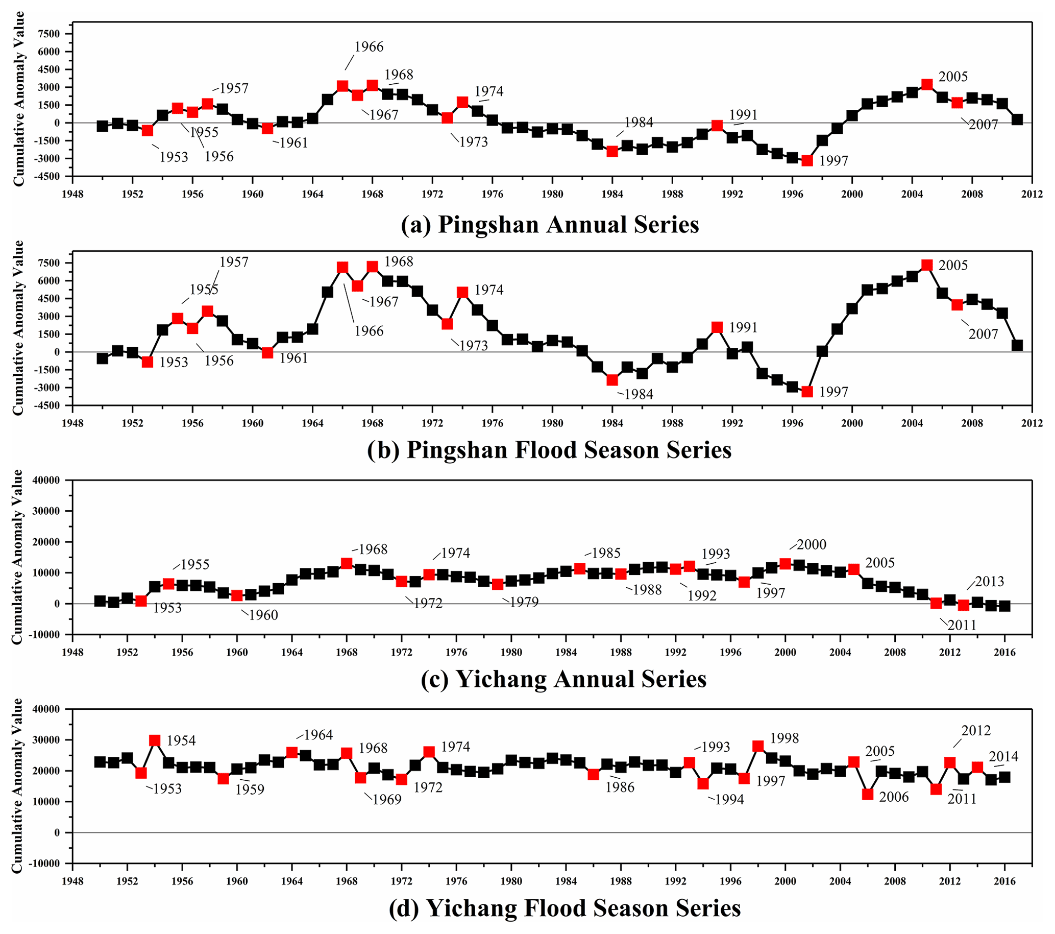
Figure 3 Potential change points of the cumulative anomaly method at Pingshan station and Yichang station.

Figure 4 Potential change points of the M-K test at Pingshan station and Yichang station.

The number of potential change points of 4-Series detected by the cumulative anomaly method is 15, 15, 16 and 18 (Fig. 3). However, the number detected by the M-K test is 2, 2, 0 and 0 (Fig. 4). In addition, there are differences in the potential change-point detection results between the annual series and the flood season series, indicating that the cumulative anomaly method has a certain response ability to flow changes. However, the consistent rate of potential change points in Pingshan station is 100 %, while Yichang station is 37.5 % and 33.33 %, respectively. This means that the response ability can only be reflected when the flow variation reaches a certain extent.

The change-point detection results of M-K test at Pingshan station (Fig. 4a and b) are concentrated around 1956 and 2005. During the same timescale, the intersection of the flood season series is slightly later than the annual series, but the amplitude of $U_{F_k}$ and $U_{B_k}$ is lower, which indirectly reflects the flood season in Pingshan station being relatively gentle, but the difference between the wet and dry seasons of the year is obvious. The YFSS is the opposite. In addition, the detection results of M-K test for 4-Series are basically consistent, insensitive to flow variation. The detected number of potential change points is small. It can be included that the cumulative anomaly method is more suitable for constructing the potential change-point set of HTS. A more accurate locating of the change point needs other methods.

4.1.2 Results of wavelet change-point detection

Among the 16 commonly used MWT systems, 8 of them satisfy the biorthogonality (59 MWT systems in total). In this study, 59 MWT systems were used to detect the potential change points of 4-Series one by one, and the number of decomposition layers used is five. However, only five MWT systems can detect the change points of 4-Series, as shown in Table 3.

Table 3 Wavelet change-point detection results of biorthogonal MWT at Pingshan station and Yichang station (number of decomposition layers is 5). Bold font represents the optimal MWT or change point. The number represents the HTS corresponding to the optimal MWT or change point.

The change point and the optimal MWT are marked with the same number (in the upper right corner) as the series.

From Table 3, the number of potential change points detected by a single MWT is between 1 and 3. The top two potential change points of the PAS are 1992 and 1999, of the PFSS 1999 and 2000, of the YAS 1961 and 1968, and of the YFSS 1975 and 2005. The number of 4-Series of change points detected is 19, 18, 19 and 17 respectively. Compared with the cumulative anomaly method and M-K test, the wavelet change-point detection has the highest contribution to the construction of the potential change-point set, followed by the cumulative anomaly method.

As the MWT changes, the detection results are quite different. For the same hydrological station and the same MWT, there is also a difference in the detection results between the annual series and the flood season series, indicating that the wavelet change-point detection is very sensitive to the flow variation of HTS. Furthermore, the detection results of Pingshan station are concentrated in 1959–2000, while those of Yichang station are concentrated in 1959–2004. Compared with the series length used in the study (Pingshan 1950–2011 and Yichang 1950–2016), the detection results are susceptible to marginal effects, and the potential change points at both ends of the series (before and after 10 years) may be ignored.

4.2 Results of change-point detection

We deduplicated and sorted the above detection results as potential change-point sets for each series, with capacities of 31, 30, 31 and 28, respectively. The degree of change (p) before and after each potential change point was calculated by the K-S test. Traditional change-point detection often adopts the method of traversal series. Take PAS as an example (62 years in total); because the starting point, change point and end point are changing, its p value is calculated ${\sum }_{n=\mathrm{1}}^{\mathrm{60}}{\sum }_{i=\mathrm{1}}^{n}i=\mathrm{35}\mathrm{990}$ times. After constructing the potential change-point set, the number of calculation is reduced to ${\sum }_{n=\mathrm{1}}^{\mathrm{29}}{\sum }_{i=\mathrm{1}}^{n}i=\mathrm{4060}$, and the efficiency is improved by 88.72 %, and the calculation results are shown in Fig. 5a. The change-point trajectories (marked with red lines and blue dots) and alternative trajectories of 4-Series were determined according to the detection criteria in Sect. 2.3, as shown in Fig. 5b and c.

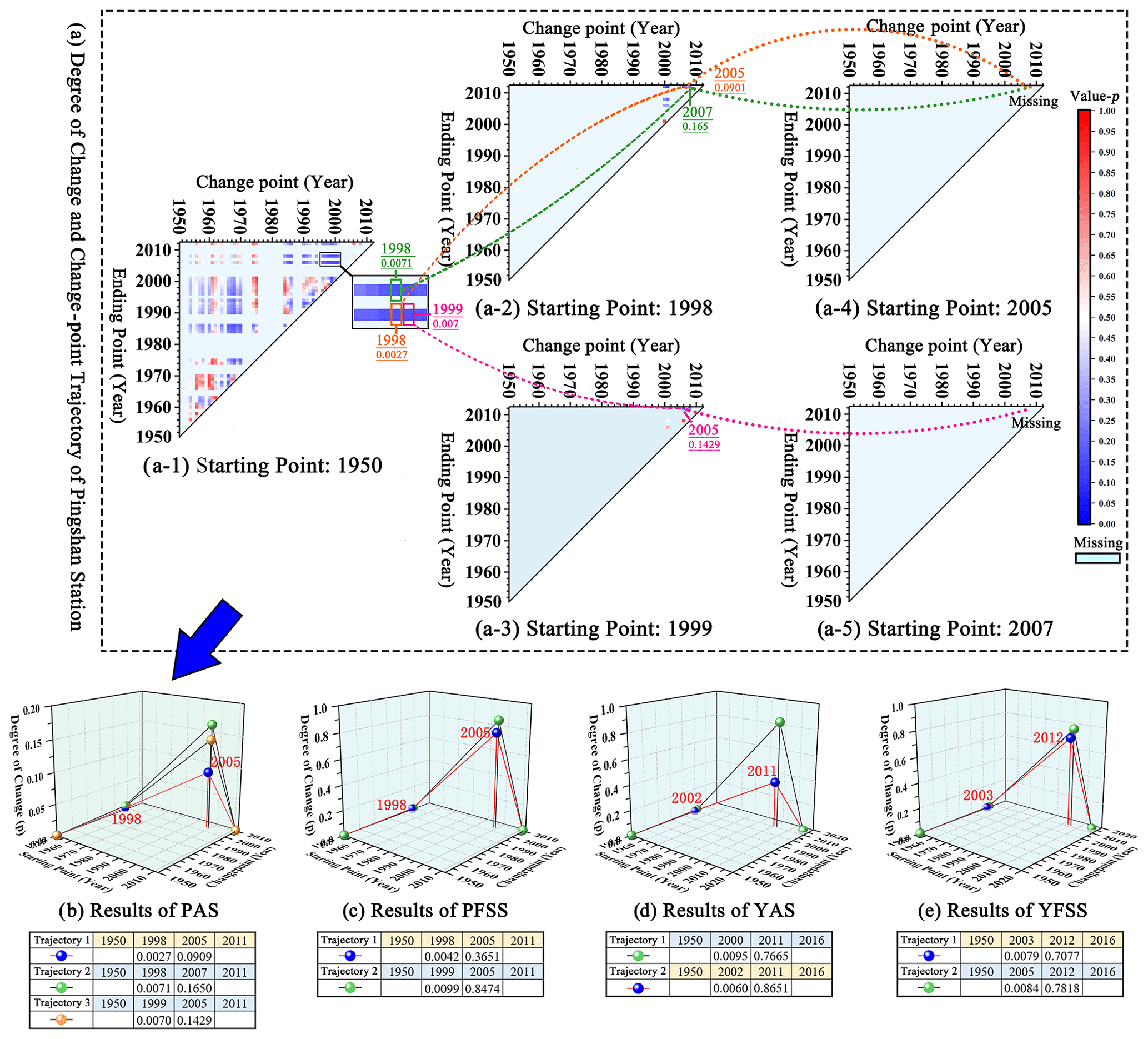
Figure 5 Change-point trajectory of Pingshan station and Yichang station (confidence level 99 %).

For PAS, the starting point of the change-point trajectory is 1950. We need to find the grid point with p<0.01 in Fig. 5a-1. Then, with the change point as the starting point and the ending point as the change point, find the grid point with p<0.01 until 2011. At a confidence level of 99 %, there are three points in Fig. 5a-1 that meet the requirements of Criterion 1, namely 1950–1998–2005 (Trajectory 1), 1950–1998–2007 (Trajectory 2) and 1950–1999–2005 (Trajectory 3), and p is shown in Fig. 5b. It can be seen that Criterion 1 can effectively narrow the selection range of change points from many potential points. Criterion 2 requires further search extending to 2011, which can fully explore the change point and ensure the continuity of the trajectory. When there are multiple alternative trajectories with an inconsistent number of change points, Criterion 3 requires to select the one with the most points, which helps to divide the series in detail. Figure 5b–e show all alternative trajectories that meet the requirements of the above three detection criteria. According to Criterion 4, select the year with small p of the first M−1 change points one by one, which can make the series before and after the change point have a large degree of change.

Based on the change-point detection criteria, the year in which the series consistency has changed due to human factors (water storage of large reservoirs, etc.) can be determined (Fig. 5b–e red line). The change-point trajectory of PFSS is consistent with PAS, while YFSS lags behind YAS by 1 year. The reason could be related to the interannual variation of runoff. The flood season of Pingshan station is from June to November, accounting for 81.34 % of the annual average runoff. The upstream Ertan Reservoir (water storage in May 1998) has seasonal regulation capacity, so it can have a direct impact on PFSS, which is divided into 1950–1997, 1998–2004 and 2005–2011. However, the flood season of Yichang station is from May to October, and the runoff in May accounts for 7.1 % of the year. The annual mean runoff from 2001 to 2004 is 13154.73, 12454.25, 12991.84 and 13115.10 m³ s⁻¹ respectively. The monthly mean runoff in flood season from 2001 to 2004 is 20010.98, 18895.22, 20690.22 and 19841.30 m³ s⁻¹ respectively. For the hydrological regime, 2002 is a year with less water inflow, while 2003 is the opposite. However, affected by the Three Gorges Reservoir, the water inflow in 2002 is closer to 2003–2010 in the flood season series, while the annual series is closer to 1950–2001. It indirectly shows that the change-point detection framework proposed in this study considers the influence of both human factors and hydrological regime on the series. The HTS division results of Pingshan station and Yichang station are shown in Fig. 5b–e. Dividing series helps ensure consistency of HTS and provides a basis for better information mining through statistical analysis methods.

4.3 Results of MWT optimization

Based on the change-point trajectories, the detection accuracy of the three methods was calculated, and the MWT optimization can be completed according to the optimization framework in Sect. 2.4. The screening process is shown in Table 3, and the optimization results of MWT are shown in Table 4.

Table 4 Change point and optimal MWT of Pingshan station and Yichang station (Confidence Level 99 %).

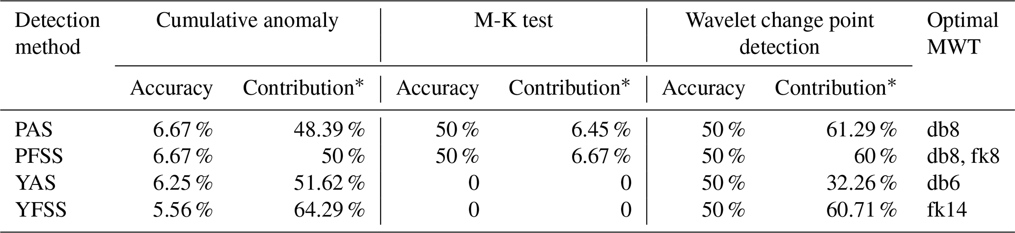
^∗ Contribution refers to the percentage of change points provided by the detection method for the potential change-point set.

Combining the MWT optimization results in Tables 3 and 4, it is found that the change point is the key to series division, and optimization step (1) can quickly locate the MWT that conforms to the series characteristics. For Pingshan station, the annual series of MWT meeting optimization step (1) is db8, and the flood season series are db8 and fk8. The optimization step (2) is selected according to the runoff physical cause at the same station, which makes it easier to analyse the evolution of the two series from the time–frequency space of the same MWT. Therefore, the optimal MWT of PFSS is db8.

When the optimal MWT of the series is determined, the accuracy of wavelet change-point detection is generally higher than the cumulative anomaly method and the M-K test (Table 4). Except for YAS, the contribution rate of wavelet change-point detection to the overall potential change point is also higher than both of them. The results show that the MWT optimization framework proposed in this study can accurately screen the optimal MWT of each series. The wavelet transform based on the MWT conforming to the series characteristics is helpful to improve the rationality of the analysis.

4.4 Analysis of HTS evolution based on CWT

Based on the optimization results of MWT in Table 4, the evolution of 4-Series was analysed by CWT. To further explore the influence of MWT, Haar, Morlet and Mexican hat (referred to as three common wavelets) were used in CWT of PAS, as shown in Fig. 6a. The analysis results of the optimal MWT are shown in Fig. 6b–e.

Figure 6 Results of CWT at Pingshan station and Yichang station (wavelet variance and real part of a contour map, with a confidence level of 99 %).

The three common wavelets have great differences in the analysis results of the main periods of PAS, namely 10a and 35a, 10a and 29a, and 3a and 10a (Fig. 6a). Furthermore, they frequently alternate between wet and dry in the short time period and exhibit a distinct “wet–dry–wet” evolution over the long time period. Compared with Fig. 6b, the CWT of three common wavelets is relatively scattered in the timescale of 0 to 60a, and the Morlet and Mexican hat wavelets show a wet period after 1998, which does not reflect the regulation effect of the Ertan Reservoir on Pingshan station, and the accuracy of the analysis results is questionable. According to historical records, during the flood season in June 1998, a basin-wide flood occurred in the middle and lower Yangtze River due to continuous heavy rain in Dongting Lake and Panyang Lake below Yichang station (Zhang et al., 2021). From the timescale (Fig. 6b and c), Pingshan station and Yichang station suffer continuous dry years, which is consistent with the actual situation. Based on the analysis of integrated moisture transport, land-falling atmospheric rivers geometric metrics and large-scale climatic circulations, Ayantobo et al. (2022) believed that the extreme rainfall in the Yangtze River basin had a declining period after 1999, which was consistent with the analysis results of this study. We believe that optimizing the MWT that conform to series characteristics based on the change-point detection is a suitable approach.

According to the analysis, the main periods of PAS are 10a and 30a, and the flood season series are 10a and 29a. The long-period scale of flood season is slightly earlier than the annual series, indicating that the annual adjustment of Pingshan station has a certain buffer capacity. On the short-period scale 10a, the two series show the phenomenon of frequent alternation of wet and dry seasons, but the consecutive dry seasons from 1926 to 1968 and 1998 to 2004 have a serious impact on the series. Especially after 1998, due to the operation of Ertan Reservoir, the runoff reduction in the annual series is larger than that in flood season, so attention should be paid to the annual water demand of river channels and cities along the route. From 2005 to 2011, Pingshan station had the wet season, and attention should be paid to flood control and flood resource utilization. The main periods of YAS are 9a and 27a, and the main periods of flood season series are 9a and 31a. Similarly, Yichang station frequently alternates between wet and dry on the short-period scale. The annual series shows the evolution of “wet–dry–wet–dry–wet” on the long-period scale, while the flood season series shows “wet–dry–wet–dry”. After 2002–2003, YFSS did not enter the wet season as the annual series, indicating that the operation of the Three Gorges Reservoir has a large reduction in the flood season. On the premise of ensuring the storage of the downstream reservoir at the end of the flood season, it is helpful to adjust the annual and interannual distribution of the runoff in the Yangtze River and improve the utilization efficiency of water resources.

5 Conclusion

Hydrological time series (HTS) is the basis of water conservancy project planning and construction. However, under the multiple effects of human activities and other factors, the consistency of HTS is destroyed. It is necessary to analyse its evolution to ensure the rationality of hydrological and hydraulic calculation. Wavelet transform is one of the widely used analysis tools of evolution in hydrology, but the its analysis accuracy is closely related to mother wavelet (MWT). To solve these two problems, with the help of the cumulative anomaly method, the Mann–Kendall (M-K) test and wavelet change-point detection, we proposed the change-point detection criteria and a MWT optimization framework in this study and took Pingshan station and Yichang station on the Yangtze River as study cases to test their effectiveness. The main conclusions are as follows:

1. Change-point detection criteria. Based on the three change-point detection methods, a potential change point set of HTS is constructed, which can make up for the limitations of a single method affected by factors such as parameter settings and marginal effects and improve the calculation efficiency. In addition, with the help of the Kolmogorov–Smirnov (K-S) test, we proposed the detection criteria to quickly confirm the change-point trajectory from the beginning to the end of HTS. While ensuring the uniqueness of the result, the change point formed by the combined action of multiple factors can be accurately identified to complete the series division.

2. MWT optimization framework. Based on the change-point detection accuracy of wavelet change-point detection, the MWT consistent with the series characteristics can be selected to ensure the accuracy of wavelet transform to analyse the HTS evolution and provide a good basis for hydrological and hydraulic calculation.

It is found that the change points of the Pingshan annual series and the Pingshan flood season series both are 1998 and 2005, the Yichang annual series are 2002 and 2011, and the Yichang flood season series are 2003 and 2012. In addition, the optimal MWT of 4-Series is db8, db8, db6 and fk8 respectively. The Ertan Reservoir has a greater impact on the annual runoff of Pingshan station, while the Three Gorges Reservoir only reduces the runoff of the Yichang station to a large extent during the flood season. Limited by the data, we did not explore the evolution of the two stations after 2017. It is also found that the wavelet change-point detection is not sufficient enough to detect the potential change point of 10 years before and after the series.

Appendix A

Table A1 Acronym list.