Using normalised difference infrared index patterns to constrain semi-distributed rainfall–runoff models in tropical nested catchments

A parsimonious semi-distributed rainfall–runoff model has been developed for flow prediction. In distribution, attention is paid to both the timing of the runoff and the heterogeneity of moisture storage capacities within sub-catchments. This model is based on the lumped FLEXL model structure, which has proven its value in a wide range of catchments. To test the value of distribution, the gauged upper Ping catchment in Thailand has been divided into 32 sub-catchments, which can be grouped into five gauged sub-catchments at which internal performance is evaluated. To test the effect of timing, first the excess rainfall was calculated for each sub-catchment, using the model structure of FLEXL. The excess rainfall was then routed to its outlet using the lag time from the storm to peak flow (TlagF) and the lag time of recharge from the root zone to the groundwater (TlagS), as a function of catchment size. Subsequently, the Muskingum equation was used to route sub-catchment runoff to the downstream sub-catchment, with the delay time parameter of the Muskingum equation being a function of channel length. Other model parameters of this semi-distributed FLEX-SD model were kept the same as in the calibrated FLEXL model of the entire upper Ping River basin (UPRB), controlled by station P.1 located at the centre of Chiang Mai province. The outcome of FLEX-SD was compared to the (1) observations at the internal stations, (2) calibrated FLEXL model, and (3) the semi-distributed URBS model – another established semi-distributed rainfall–runoff model. FLEX-SD showed better or similar performance during calibration and especially in validation. Subsequently, we tried to distribute the moisture storage capacity by constraining FLEX-SD on patterns of the NDII (normalised difference infrared index). The readily available NDII appears to be a good proxy for moisture stress in the root zone during dry periods. The maximum moisture-holding capacity in the root zone is assumed to be a function of the maximum seasonal range of NDII values and the annual average NDII values to construct two alternative models, namely FLEX-SD-NDII_MaxMin and FLEX-SD-NDII_Avg. The additional constraint on the moisture-holding capacity (Sumax) by NDII, particularly in FLEX-SD-NDII_Avg, improved both the model performance and the realism of its distribution across the UPRB, which corresponds linearly to the percentage of evergreen forests (R²=0.69). To check how well the models represents simulated root zone soil moisture (Su_i), the performance of the FLEX-SD-NDII models was compared to the time series of the soil water index (SWI). The correlation between the Su_i and the daily SWI appeared to be very good and was even better than the correlation with the NDII, which does not provide good estimates during wet periods. The SWI, which is model-based, was not used for calibration but appeared to be an appropriate index for validation.

1 Introduction

Runoff is one of the most important components of the hydrological cycle and can be monitored by the installation of a gauging station. Unfortunately, only a limited number of high-quality gauging stations are available due to topographic, financial, and human resources limitations. A wide variety of rainfall–runoff models has been developed in gauged and ungauged catchments in different parts of the globe. Most rainfall–runoff models are categorised as lumped models, which provide runoff estimates only at the site of calibration. These models include FLEXL, FLEX-Topo (Euser et al., 2015; Gao et al., 2014), NAM (Bao et al., 2011; Tingsanchali and Gautam, 2000; Vaitiekuniene, 2005; Yew Gan et al., 1997), SCS (Hawkins, 1993; Lewis et al., 2000; Mishra et al., 2005; Suresh Babu and Mishra, 2011; Yahya et al., 2010), and others. Among the wide range of existing lumped rainfall–runoff models, FLEXL has proven to be an adequate model for runoff estimation in a wide range of catchments (Fenicia et al., 2008, 2011; Gao et al., 2014; Kavetski and Fenicia, 2011; Tekleab et al., 2015). This model was further developed by Gharari et al. (2011) and Gao et al. (2016) to account for the spatial variability in landscape characteristics (FLEX-TOPO), which is useful for prediction in ungauged basins (Savenije, 2010).

However, the generation of runoff exhibits the spatial and temporal variability in nature, which is not effectively accounted for by the conceptualisation of lumped models. Hence, the distribution of key routing and storage parameters is implemented in semi-distributed frameworks to better understand their effects on the partitioning of moisture and water balance. The URBS model accounts for the spatiotemporal variability in rainfall by separating the catchment of interest into a series of sub-catchments (Mapiam and Sriwongsitanon, 2009). This framework allows runoff to be estimated at any required upstream location (Carroll, 2004; Malone, 1999), thus providing useful application for real-time flood forecasting in a variety of catchments in Australia and globally (Malone, 2006; Malone et al., 2003; Mapiam and Sriwongsitanon, 2009; Mapiam et al., 2014; Rodriguez et al., 2005; Sriwongsitanon, 2010). But accounting for distributed routing and storage parameters alone does not address the variability in moisture storage capacities across heterogeneous sub-catchments, which is a key parameter for runoff generation. For this reason, room for improvement with respect to the realism of conceptual hydrological models lies within their effectiveness at better capturing the variability in moisture stresses.

The fact that remote sensing (RS) proxies for moisture storage are available in ungauged basins makes RS an essential additional data source for distributed modelling, even though such proxies themselves have intrinsic model-based uncertainties. Remote sensing observation techniques have been demonstrated in several studies to account for the spatial patterns of different vegetation types and moisture states, such that they could be valuable in constraining semi-distributed hydrological models (e.g. Savenije and Hrachowitz, 2017).

The normalised difference infrared index (NDII) is an index that detects canopy water content (Hardisky et al., 1983), which has recently been investigated for monitoring drought conditions (Moricz et al., 2018; Xulu et al., 2018). The index is indicative of differences in moisture capacities and has been shown to correspond with root zone soil moisture (RZSM) dynamics. Sriwongsitanon et al. (2016) used NDII as a proxy for RZSM and showed its effectiveness in eight sub-catchments of the upper Ping River basin in Thailand. This agrees with the study carried out by Castelli et al. (2019), who found reasonable correlations between Landsat 7 NDII values and the measured RZSM contents of rainfed olive trees growing in the arid regions of southeastern Tunisia. Mao and Liu (2019) found RZSM signatures to be well-correlated to NDII in most regions, except in river basins with high forest coverage, in addition to those with low moisture stress or those with trees intercepting deep groundwater (e.g. Eucalyptus). As such, the above studies reveal the worthwhileness of incorporating NDII to constrain semi-distributed models to enhance model realism, as indicated by the achieved accuracy improvements to runoff estimation. This study utilises the fundamental model structure of FLEXL, which includes the same distributed time lags and channel routing as used in URBS and includes distributed root zone soil moisture capacity per sub-catchment to create a new parsimonious semi-distributed FLEX model for flood and flow monitoring within the (ungauged) sub-catchments of the gauged upper Ping River basin. (1) To introduce the effect of runoff timing in a catchment with multiple sub-catchments, travel times to the outfall of each individual sub-catchment are computed on the basis of topographical indicators, and the routing of the discharge from the sub-catchment outfall to stations further downstream is computed using the Muskingum method. These time lags are then applied in the FLEX-SD model system and in the well-established URBS model for the purpose of comparison. These two semi-distributed models only account for timing but not for the distribution of the moisture storage capacity, which is a crucial parameter in runoff generation. The distribution of time lags is expected to properly simulate the hydrograph shape, particularly the timing and shape of the peaks of all sub-catchments within calibrated gauging station, but it does not affect the partitioning of the hydrological fluxes or the water balance and the accuracy of runoff estimates. (2) Subsequently, the effect of the distribution of the root zone moisture storage is studied in the FLEX-SD model, making use of the spatial distribution pattern of the maximum and minimum range of NDII values and the annual average NDII values to construct two alternative models, namely FLEX-SD-NDII_MaxMin and FLEX-SD-NDII_Avg. (3) As a validation of the realism of the hydrological models tested, as indicated by their ability to capture the variability in internal moisture states across sub-catchments, the derived simulated root zone moisture storages are compared to the independent time series of the model-based soil water index (SWI) and the RS-based NDII.

2 Study area and datasets

2.1 Study area

The upper Ping River basin (UPRB) is situated between 17^∘14^′30^′′ to 19^∘47^′52^′′ N and 98^∘4^′30^′′ to 99^∘22^′30^′′ E in the provinces of Chiang Mai and Lamphun. The catchment area of the basin is approximately 25 370 km². The basin is dominated by well-forested, steep mountains, generally in a north–south alignment (Sriwongsitanon and Taesombat, 2011). The areal average annual rainfall and runoff of the basin from 2001–2016 is 1224 and 235 mm yr⁻¹, respectively. The land use for the UPRB in 2013 can be classified into six main classes comprising forest, irrigated agriculture, rainfed agriculture, bare land, waterbody, and others, which cover approximately 77.40 %, 3.11 %, 12.54 %, 1.99 %, 1.23 %, and 3.73 % of the catchment area, respectively (Land Development Department, LDD). The landform of the UPRB varies from an undulating to a rolling terrain, with steep hills at elevations of 1500–2000 m, and valleys of 330–500 m (Mapiam and Sriwongsitanon, 2009; Sriwongsitanon, 2010). The Chiang Dao district, north of Chiang Mai, is the origin of the Ping River, which flows downstream to the south to become the inflow of the Bhumibol Dam – a large dam with an active storage capacity of about 9.7 × 10⁹ m³ (Sriwongsitanon, 2010). The climate of the basin is dominated by tropical monsoons. The southwestern monsoon causes a rainy season between May and October, and the northeastern monsoon brings dry weather and low temperatures between November and April. Only 6142 km² of the total area controlled by the runoff station P.1 (situated at the centre of Chiang Mai) is selected for this study (Fig. 1). The catchment area of the station P.1 is divided into 32 sub-catchments (Fig. 1), which is where the semi-distributed rainfall–runoff models are tested.

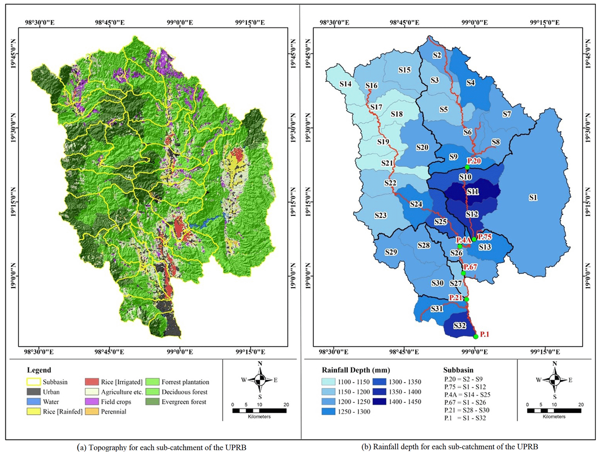
Figure 1 Topography and mean annual rainfall depth for each sub-catchment of the UPRB.

2.2 Rainfall data

Daily rainfall data from 48 non-automatic rain gauge stations located within the UPRB and its surroundings from 2001–2016 were used in this study. These data are owned and operated by the Thai Meteorological Department and the Royal Irrigation Department. These data have been validated for their accuracy on a monthly basis using double mass curve, and some inaccurate data were removed from the time series before spatially averaging using an inverse distance square (IDS) to be applied as the forcing data of URBS, FLEXL, and FLEX-SD. Mean areal rainfall depth for each of 32 sub-catchments varies between 1100 (S17) and 1402 mm yr⁻¹ (S11), as shown in Fig. 1b, while the average rainfall depth of P.1 is approximately 1224 mm yr⁻¹.

2.3 Runoff data

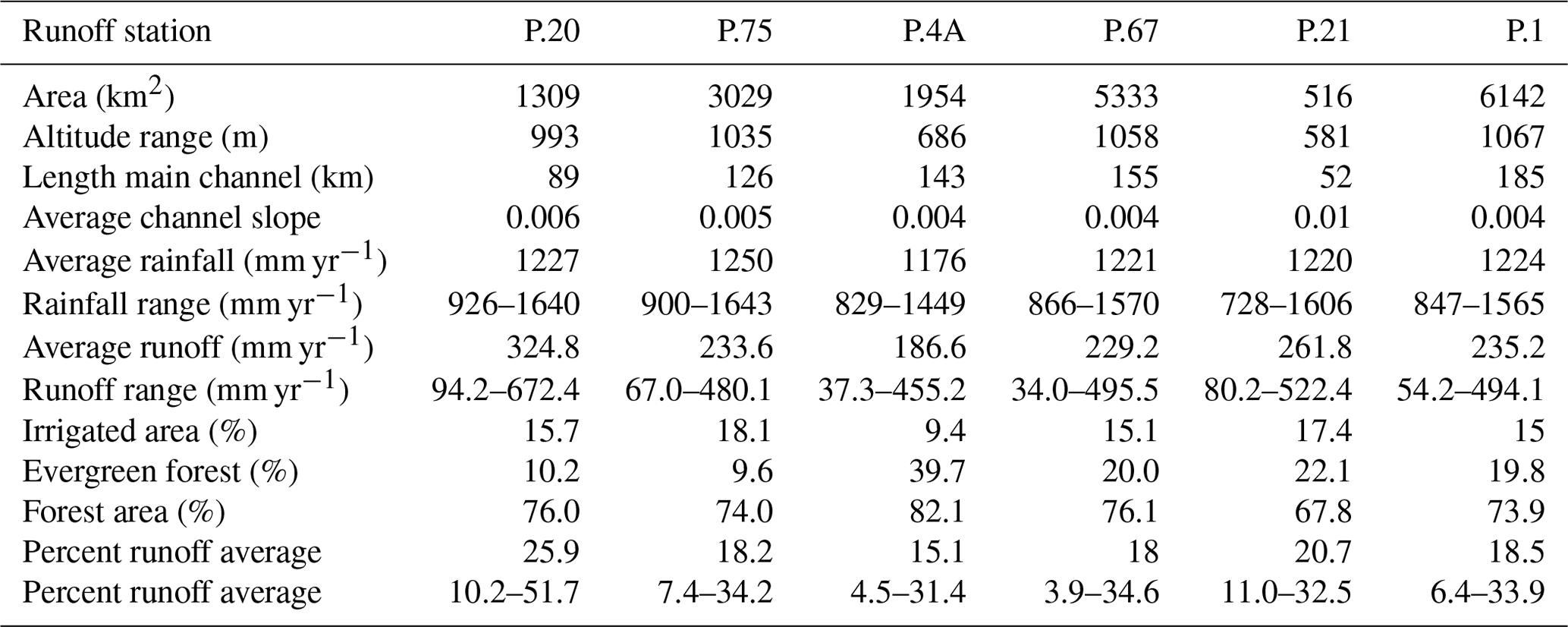
The Royal Irrigation Department (RID) operated seven daily runoff stations in the study area between 2001 and 2016, as shown in Fig. 1. Catchment P.56A was rejected from the study because it is located upstream of the Mae Ngat reservoir. Outflow data from the reservoir were used as input data in model calibration. Runoff data at the remaining six stations were used for the study, since they are not affected by large reservoirs. The data have been checked for their accuracy by comparing them with average rainfall data covering their catchment areas at the same periods. Table 1 presents the catchment characteristics and hydrological data for these six gauging stations in the UPRB. In this study, the catchments of these six stations were divided into 32 sub-catchments (see Fig. 1), with areas ranging from 57 to 230 km². High variation in catchment size is due to the proximity between the locations of these runoff stations and the outlets of the tributaries. Runoff data have been checked for their accuracy by comparing the annual runoff coefficient between all stations. The comparison revealed that the runoff coefficients at P.20 in 2006 and 2011 are overestimated, while the runoff coefficient at P.21 in 2004 is underestimated, and in 2007 and 2009, the runoff coefficients are overestimated due to the incorrect rating curves (see Fig. 2). These inaccurate data would affect the results of the model calibration.

Figure 2 Runoff coefficient of each station.

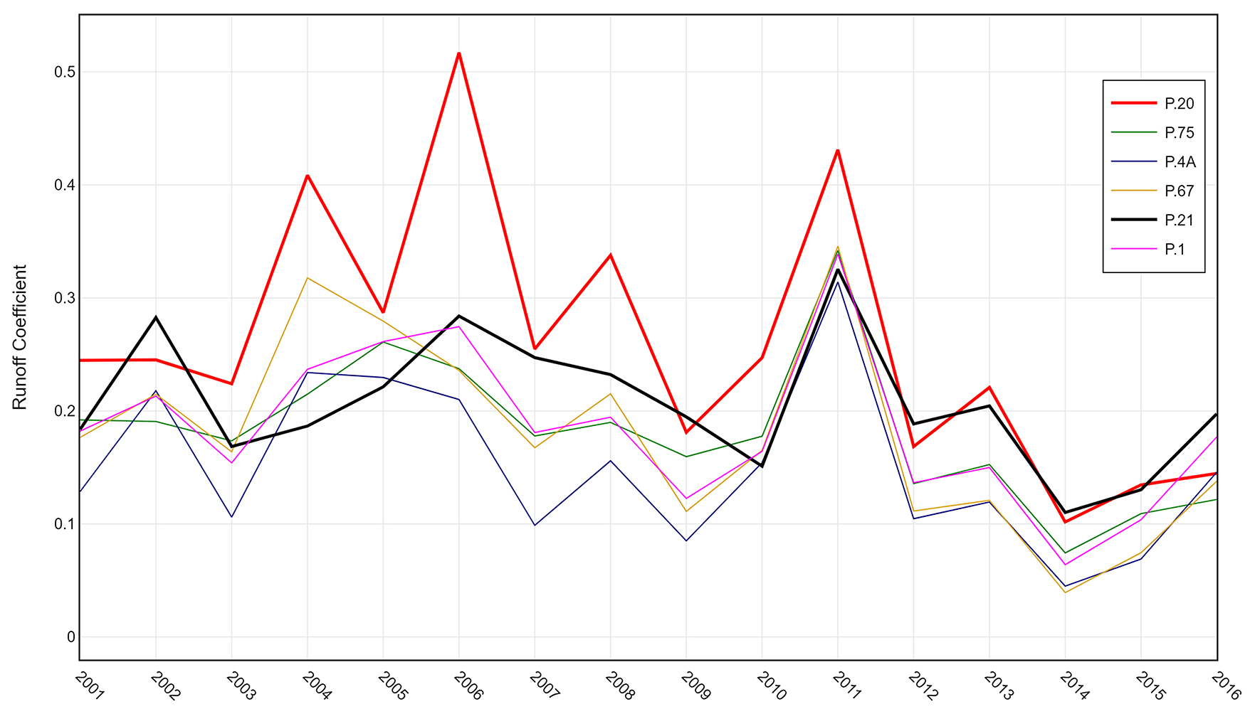
Table 1 Catchment characteristics and hydrological data for six gauging stations in the study area.

2.4 NDII data

The normalised difference infrared index (NDII) is a ratio of the near-infrared (NIR) and shortwave infrared (SWIR) bands, centred at 859 and 1640 nm, respectively, as shown in Eq. (1). In this study, the NDII was calculated using the MODIS level 3 surface reflectance product (MOD09A1), which is available at 500 m resolution in an 8 d composite of the gridded level 2 surface reflectance products. Atmospheric correction has been carried out to improve the accuracy and can be downloaded from ftp://e4ftl01.cr. usgs.gov/MOLT (last access: 14 November 2020; Vermote et al., 2011). The 8 d NDII values between 2002–2016 were averaged over each of 31 sub-catchments of the UPRB to be used for estimating the model parameter within sub-catchment and for it to be compared to the 8 d average Su (root zone storage) values extracted from the model results at each station.

$$\begin{array}{}\text{(1)}& \mathrm{NDII}={\displaystyle \frac{(\mathrm{NIR}-\mathrm{SWIR})}{(\mathrm{NIR}+\mathrm{SWIR})}}\end{array}$$

2.5 SWI data

The near-real-time SWI is derived from the reprocessed surface soil moisture (SSM) data derived from the Advanced SCATterometer (ASCAT) sensor (Brocca et al., 2011; Paulik et al., 2014), which is a C-band scatterometer measuring at a frequency of 5.255 GHz in vertical transmit and receive polarisation (VV) (Paulik et al., 2014). The product makes use of a two-layer water balance model to describe the time series relationship between surface and profile soil moisture. This dataset of moisture conditions is available on a daily basis for eight characteristic time windows (1, 5, 10, 15, 20, 40, 60, and 100 d). The global-scale SWI dataset is available at 0.1^∘, which is about 10 km resolution, within 3 d after observation and can be downloaded from the Copernicus Global Land Service website. The dataset is available from January 2007 onwards. Since the SWI dataset is not complete in 2007, only the data between 2008 and 2016 have been used in this study. The characteristic time length is the only parameter in the SWI procedure. Bouaziz et al. (2020) specified the optimal T values (T_opt) by matching the modelled time series of RZSM from a calibrated FLEXL model to several SWI products in 16 contrasting catchments in the Meuse river basin. They concluded that the characteristic time lengths are differentiated amongst land cover (percent agriculture), soil properties (percent silt), and runoff signatures (flashiness index). In Sect. 5.4.2, the appropriate timescale for the Ping basin will be determined in 40 d.

3 Theoretical background

3.1 FLEXL model

FLEXL is a lumped hydrological model comprising five reservoirs, namely a snow reservoir (Sw), an interception reservoir (Si), an unsaturated soil reservoir (Su), a fast-response reservoir (Sf), and a slow-response reservoir (Ss; Gao et al., 2014). Excess rainfall from a snow reservoir, an interception reservoir, and an unsaturated soil reservoir is divided and routed into a fast-response reservoir and a slow-response reservoir using two lag functions. It includes the lag time from storm to peak flow (TlagF) and the lag time of recharge from the root zone to the groundwater (TlagS). Each reservoir has process equations that connect the fluxes entering or leaving the storage compartment to the storage in the reservoirs (so-called constitutive functions; Sriwongsitanon et al., 2016). The water balance equations and constitutive equations for each conceptual reservoir are summarised in Fig. 3 and Table 2. The total number of model parameters is 11. Forcing data include the daily average rainfall and potential evaporation derived by the Penman–Monteith equation.

Figure 3 Model structure of FLEXL model.

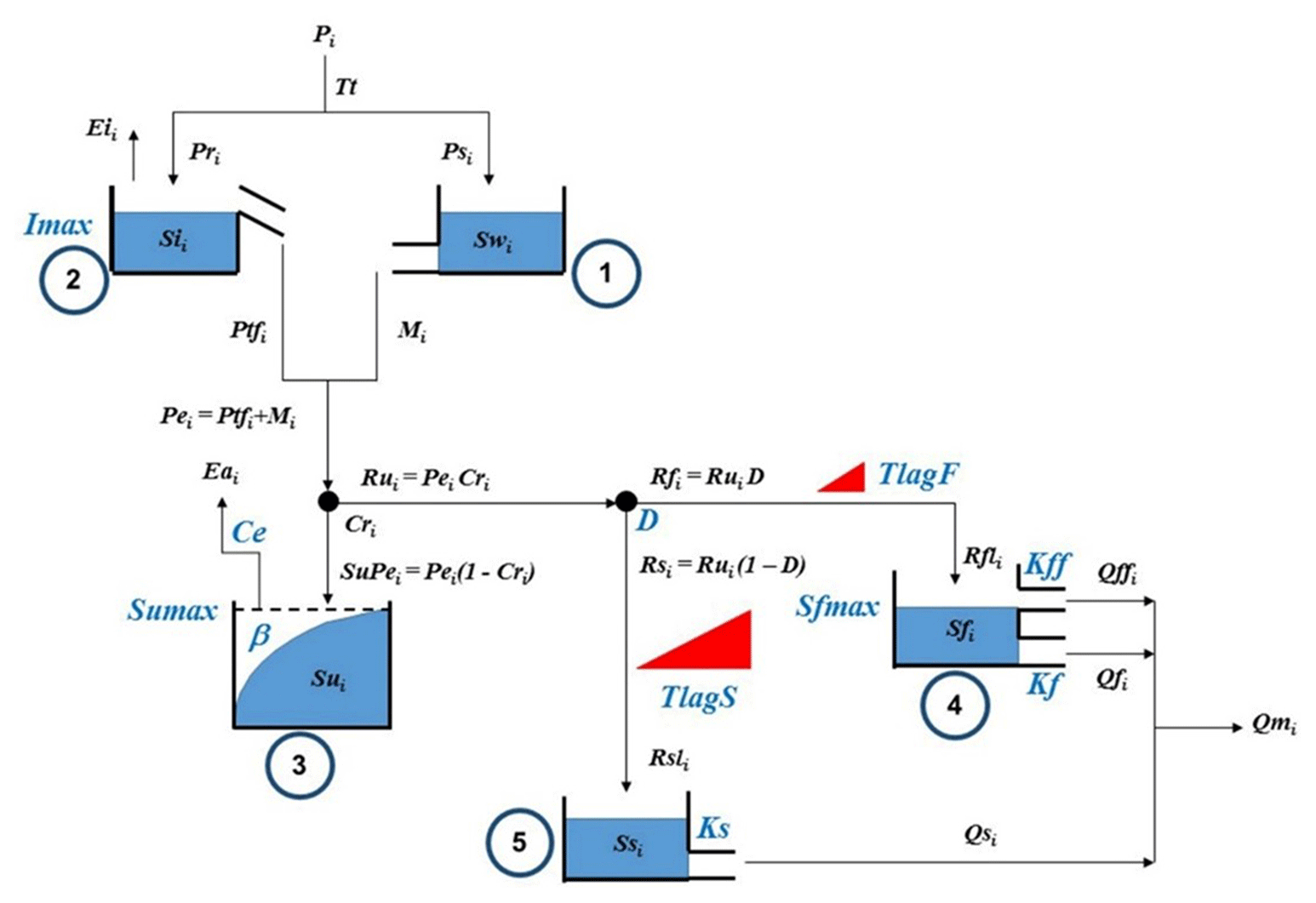
Table 2 Constitutive and water balance equations used in FLEXL.

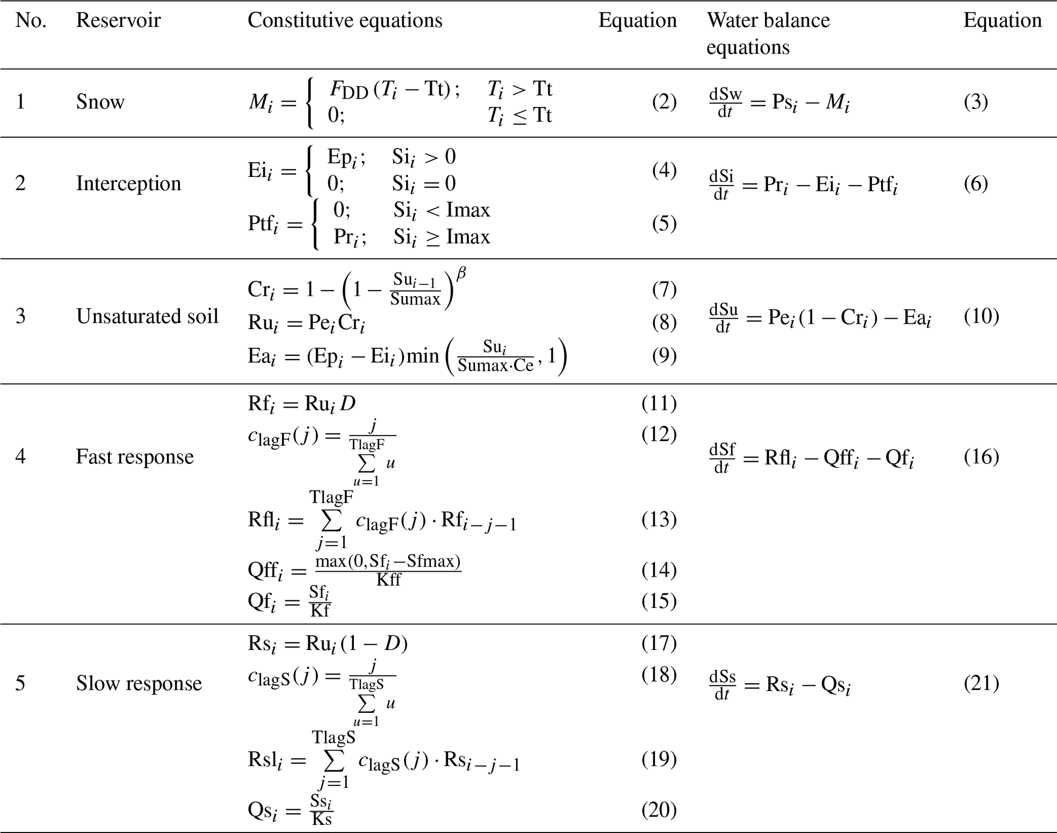
3.1.1 Snow reservoir

The snow routine, which is not very relevant in Thailand, can play an important role in areas with snow. When there is snow cover and the temperature (T_i) is above Tt, then the effective precipitation is equal to the sum of the rainfall (P_i) and snowmelt (M_i). The snowmelt (M_i) is calculated by the melted water per day per degree Celsius above Tt (F_DD; Eq. 2). The snow reservoir uses the water balance equation, Eq. (3), where Sw_i (mm) is the storage of the snow reservoir.

3.1.2 Interception reservoir

Interception is more important in summer and autumn. The interception evaporation (Ei_i) was calculated by the potential evaporation (Ep_i) and the storage in the interception reservoir (Si_i), with a daily maximum storage capacity (Imax; Eqs. 4 and 5). The interception reservoir uses the water balance equation, Eq. (6), as presented in Table 2.

3.1.3 Root zone reservoir

The root zone routine, which is the core of the hydrological models, determines the amount of runoff generation. In this study, we applied the widely used beta function of the Xinanjiang model (Ren-Jun, 1992) to compute the runoff coefficient for each time step as a function of the relative soil moisture. In Eq. (7), Cr_i indicates the runoff coefficient, Su_i is the storage in the root zone reservoir, Sumax is the maximum moisture-holding capacity in the root zone, and β is the parameter describing the spatial process heterogeneity of the runoff threshold in the catchment. In Eq. (8), Pe_i indicates the effective rainfall and snowmelt into the root zone routine, and Ru_i represents the generated flow during rainfall events. In Eq. (9), Su_i, Sumax, and potential evaporation (Ep_i) were used to determine the actual evaporation from the root zone Ea_i; Ce indicates the fraction of Sumax above which the actual evaporation is equal to potential evaporation, which is set here to 0.5, as previously suggested by Savenije (1997). Otherwise, Ea_i is constrained by the water available in Su_i. The unsaturated soil reservoir uses the water balance equation, Eq. (10), as presented in Table 2.

3.1.4 Fast-response reservoir

In Eq. (11), Rf_i indicates the flow into the fast-response routine, and D is a splitter to separate the recharge from preferential flow. Equations (12) and (13) were used to describe the lag time between storm and peak flow. Rf${}_{t-i+\mathrm{1}}$ is the generated fast runoff in the unsaturated zone at time $t-i+\mathrm{1}$, TlagF is a parameter which represents the time lag between storm and fast-runoff generation, c_lagF(i) is the weight of the flow in i−1 days before, and Rfl_i is the discharge into the fast-response reservoir after convolution.

A linear-response reservoir, representing a linear relationship between storage and release, was applied to conceptualise the discharge from the surface runoff reservoir, fast-response reservoirs and slow-response reservoirs. In Eq. (14), Qff_i is the surface runoff, with timescale Kff, which is active when the storage of the fast-response reservoir exceeds the threshold Sfmax. In Eq. (15), Qf_i represents the fast runoff, Sf_i represents the storage state of the fast-response reservoirs, and Kf is the timescales of the fast runoff. The fast-response reservoir uses the water balance equation, Eq. (16), as presented in Table 2.

3.1.5 Slow-response reservoir

In Eq. (17), Rs_i indicates the recharge of the groundwater reservoir. Equations (18) and (19) were used to describe the lag time of recharge from the root zone to the groundwater. Rs${}_{t-i+\mathrm{1}}$ is the generated slow runoff in the groundwater zone at time $t-i+\mathrm{1}$, TlagS is a parameter which represents the lag time of recharge from the root zone to the groundwater, c_lagS(i) is the weight of the flow in i−1 days before, and Rsl_i is the discharge into the slow-response reservoir after convolution. In Eq. (20), Qs_i represents the slow runoff, Ss_i represents the storage state of the groundwater reservoir, and Ks is the timescale of the slow runoff. The slow-response reservoir uses the water balance equation, Eq. (21), as presented in Table 2.

3.2 URBS model

URBS was developed by the Queensland Department of Natural Resources and Mines in 1990, based on the structures of RORB (Laurenson and Mein, 1990) and WBNM (Boyd et al., 1987). URBS is a semi-distributed rainfall–runoff model that can provide runoff estimates not only at the calibrated station but also at the outlet of every sub-catchment at any required location upstream. The calibrated catchment area needs to be divided into sub-catchments to obtain different areal rainfall and different catchment and channel travelling time.

Table 3 presents five main processes used in URBS, comprising the calculation of the initial loss, proportional loss, excess rainfall, catchment routing, and channel routing. Excess rainfall is calculated separately between the pervious and impervious areas. For the pervious area, URBS assumes that there is a maximum initial loss rate (IL_max) to be reached before any rainfall can become the effective rainfall ($R_i^{\mathrm{eff}}$). The initial loss (IL_i) can be recovered when the rainfall rate (R_i) is less than the recovering loss rate (rlr) per time interval (δt; see Eq. 22).

Table 3 Constitutive equations used in URBS.

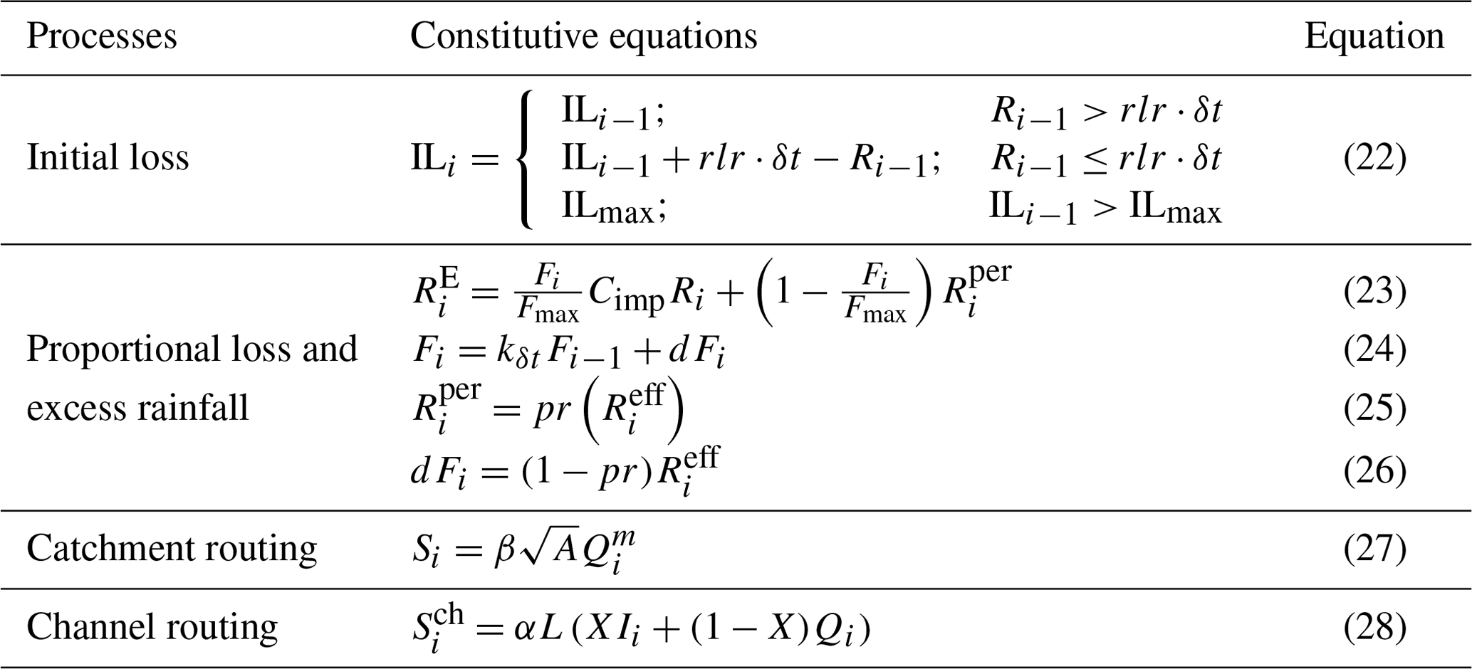
Excess rainfall for each time step is calculated using Eq. (23), by weighting the excess rainfall between pervious and impervious area using a ratio of the cumulative infiltration (F_i) and the maximum infiltration capacity (F_max). The recovering rate is included by simply reducing the amount infiltrated after every time step, using the reduction coefficient (k_δt), as shown in Eq. (24), and the pervious excess rainfall ($R_i^{\mathrm{per}}$) is calculated using the Eq. (25), where pr is the proportional runoff coefficient. The remaining water $(\mathrm{1}-\mathrm{pr})R_i^{\mathrm{eff}}$ will infiltrate to the root zone storage (dF_i; see Eq. 26). Excess rainfall is then routed to the centroid of any sub-catchment using a nonlinear reservoir relationship ($S_i=K{Q}_i^m$). The parameter m is the catchment nonlinearity, and K is the catchment travel time, which can be calculated for different sub-catchment using the multiplication between the catchment lag time coefficient (β) and square root of each sub-catchment area (A; see Eq. 27).

Thereafter, the outflow at the centroid of each sub-catchment is routed along a reach downstream of each sub-catchment, using the Muskingum equation ($S_i^{\mathrm{ch}}=K_{\mathrm{ch}}(X{I}_i+(\mathrm{1}-X\left)Q_i\right)$). The parameter X is the Muskingum coefficient, and K_ch is the channel travel time, which can be calculated for different sub-catchment using the multiplication between the channel lag coefficient (α) and the reach length (L) between the closest location in the channel to the centroid and the outlet of each sub-catchment (see Eq. 28).

4 Methodology

4.1 Development of the semi-distributed FLEX models

The first step in distribution is to account for the timing of floods and the rooting of flood waves as a function of topographical factors. The resulting semi-distributed FLEX-SD model is therefore expected to better represent the shape of hydrographs, although it would not affect the partitioning of fluxes or the water balance. The root zone storage capacity is a strong control on partitioning, affecting both runoff generation and evaporation. Therefore, the distribution of this parameter would potentially affect overall model performance more strongly than merely affecting the timing of the peaks. Therefore, in a second step, the NDII, as a proxy for moisture storage, is used to assess the distribution of moisture storage among sub-catchments.

4.1.1 Accounting for distributed timing and channel-routing

FLEX-SD is set up by applying lumped models for each sub-catchment, which adds up to a semi-distributed model for a downstream calibration site. Therefore, the catchment area of any gauging station needs to be divided into sub-catchments. Runoff estimates at each sub-catchment can be simulated using the structure of the original FLEXL, by calculating different excess rainfall for each sub-catchment. The excess rainfall of each sub-catchment is routed to its outlet using the lag time from rainfall to surface runoff (TlagF) and the lag time of recharge from the root zone to the groundwater (TlagS). In this study, TlagF and TlagS are calculated in hours instead of days to increase the model performance. The lag time is distributed among sub-catchments using the following equations.

$$\begin{array}{}\text{(29)}& {\displaystyle }& {\displaystyle }{\mathrm{TlagF}}_{\mathrm{sub}}=\mathrm{TlagF}\sqrt{A_{\mathrm{sub}}/A}\text{(30)}& {\displaystyle }& {\displaystyle }{\mathrm{TlagS}}_{\mathrm{sub}}=\mathrm{TlagS}\sqrt{A_{\mathrm{sub}}/A},\end{array}$$

where TlagF and TlagS are lag time parameters for the entire catchment of a calibrated gauging station. The lag time of each sub-catchment (TlagS_sub) is scaled by the square root of each sub-catchment area divided by the overall catchment area (A).

Runoff estimates from an upstream sub-catchment are later routed from their outlet to the outlet of a downstream sub-catchment using the Muskingum method (Eq. 31) before adding to the runoff estimates of the downstream sub-catchment.

$$\begin{array}{}\text{(31)}& {\displaystyle }& {\displaystyle }{S}_{\mathrm{chnl}\text{-}\mathrm{sub}}=K_{\mathrm{sub}}\left(X{Q}_{\mathrm{up}}+(\mathrm{1}-X)Q_{\mathrm{down}}\right)\text{(32)}& {\displaystyle }& {\displaystyle }{K}_{\mathrm{sub}}=\mathit{\alpha }{L}_{\mathrm{sub}},\end{array}$$

where α and X are the delay time parameter and the channel routing parameter for the entire catchment, respectively. The delay time parameter of each sub-catchment (K_sub) can be calculated by the multiplication between α and the main channel length of each sub-catchment, as shown in Eq. (32).

4.1.2 Accounting for distributed root zone storage at sub-catchment scale using the maximum and minimum values of NDII (FLEX-SD-NDII_MaxMin model)

The normalised difference infrared index (NDII) was used to estimate the root zone storage capacity for each sub-catchment. The NDII values, which are available at 8 d intervals, were found to correlate well with the 8 d average root zone moisture content (Su) simulated by FLEXL during the dry period in eight sub-catchments in the UPRB (Sriwongsitanon et al., 2016). The relation between NDII and Su can be described by an exponential function of the type ae^b(NDII)+c, with c being close to zero. The maximum value that Su can achieve is Sumax, which is the storage capacity of the root zone. The hypothesis is that the ecosystem creates sufficient storage to overcome a critical period of drought (Gao et al., 2014; Savenije and Hrachowitz, 2017). Every year has a maximum range of storage variation. If a sufficiently long NDII record is available, then the maximum of the annual ranges of the NDII should provide an estimate of the root zone storage capacity Sumax. By calibrating the hydrological FLEX model to discharge observations at the gauging stations, a Sumax value can be calibrated for each gauged catchment. This is a representative Sumax value for a particular gauging station, consisting of n sub-areas, as indicated by Sumax_n.

$$\begin{array}{}\text{(33)}& {\mathrm{Sumax}}_n={\displaystyle \frac{\sum _{i=\mathrm{1}}^n\left(A_i{\mathrm{Sumax}}_i\right)}{\sum _{i=\mathrm{1}}^n{A}_i}}\end{array}$$

By using the NDII as proxy for root zone storage, we have developed the following equation for the proxy root zone storage capacity Sumax${}_i^{\prime }$ for a sub-area within a river basin consisting of 31 sub-catchments:

$$\begin{array}{}\text{(34)}& {\mathrm{Sumax}}_i^{\prime }={\displaystyle \frac{{\left[e^{b\times {\mathrm{NDII}}_{i,\max }}-e^{b\times NDI{I}_{i,\min }}\right]}_{\max }}{{\left[e^{b\times {\mathrm{NDII}}_{n,\max }}-e^{b\times {\mathrm{NDII}}_{n,\min }}\right]}_{\max }}},\end{array}$$

where Sumax${}_i^{\prime }$ is a scaled proxy for the root zone storage capacity of each sub-catchment, and b is the remaining calibration parameter because the constant c and the factor a of the exponential function drop out. NDII_i,max and NDII_i,min represent the maximum and minimum values of NDII for each year of each sub-catchment, while NDII_n,max and NDII_n,min indicate the maximum and minimum values of NDII for each year in the reference basin, which, in this case, is the entire upper Ping basin controlled by station P.1. The unscaled root zone storage capacity per sub-catchment then becomes the following:

$$\begin{array}{}\text{(35)}& {\mathrm{Sumax}}_i={\mathrm{Sumax}}_n{\displaystyle \frac{{\mathrm{Sumax}}_i^{\prime }}{{\mathrm{Sumax}}_n^{\prime }}},\end{array}$$

where Sumax_n is the calibrated value of the root zone storage capacity of the gauged catchment, and Sumax${}_n^{\prime }$is the area-weighted proxy for the root zone storage capacity.

$$\begin{array}{}\text{(36)}& {\mathrm{Sumax}}_n^{\prime }={\displaystyle \frac{\sum _{i=\mathrm{1}}^n\left(A_i{\mathrm{Sumax}}_i^{\prime }\right)}{\sum _{i=\mathrm{1}}^n{A}_i}}\end{array}$$

4.1.3 Accounting for distributed root zone storage at sub-catchment scale using average value of NDII (FLEX-SD-NDII_Avg)

Instead of applying the maximum and minimum of the annual ranges of the NDII to distribute root zone storage at a sub-catchment scale, we tested the annual average NDII value of each sub-area to calculate Sumax${}_i^{\prime }$ as presented in the following equation.

$$\begin{array}{}\text{(37)}& \begin{array}{rl}{\mathrm{Sumax}}_i^{\prime }& =\left(\mathrm{0.5}-{\displaystyle \frac{R}{\mathrm{2}}}\right)\\ & +R\left({\displaystyle \frac{\left(e^{b\times {\mathrm{NDII}}_i}\right)-{\left(e^{b\times {\mathrm{NDII}}_{i\to n}}\right)}_{\min }}{{\left(e^{b\times {\mathrm{NDII}}_{i\to n}}\right)}_{\max }-{\left(e^{b\times {\mathrm{NDII}}_{i\to n}}\right)}_{\min }}}\right),\end{array}\end{array}$$

where NDII_i represents the annual average NDII value of each sub-catchment, while $(e^{b\times {\mathrm{NDII}}_{i\to n}}{)}_{\max }$ and $(e^{b\times {\mathrm{NDII}}_{i\to n}}{)}_{\min }$ indicate the maximum and minimum values of exponential function produced by the annual average NDII value within 32 sub-catchments. The parameters b and R can be determined by model calibration. The parameter R is suggested to vary between 0.2 and 0.8 to force a scaled factor (Sumax${}_i^{\prime }$) to be more than 0 and less than 1. The average NDII value is supposed to reflect the maximum moisture storage capacity as well, since a high maximum value also leads to a higher average but is much easier to calculate. However, this method requires the introduction of the additional calibration parameter R.

4.2 Model applications

First, FLEXL and the four semi-distributed models, URBS, FLEX-SD, FLEX-SD-NDII_MaxMin, and FLEX-SD-NDII_Avg were individually calibrated (2001–2011) and validated (2012–2016) at the stations P.4A, P.20, P.21, P.75, P.67, and P.1 to provide baselines for comparison of model performances. Furthermore, additional runoff estimates at the outlet of 31 sub-catchments, inclusive of the internal gauging stations upstream of P.1, were extracted from the four semi-distributed models. The runoff estimates at the above stations were compared to the observed data and also for their comparability to the performance of FLEXL at individual stations.

The model parameters of the calibrated models were determined using the MOSCEM-UA (Multi-Objective Shuffled Complex Evolution Metropolis–University of Arizona) algorithm (Vrugt et al., 2003), by finding the Pareto-optimal solutions defined by three objective functions of the Kling–Gupta efficiencies for high flows, low flows, and the flow duration (KGE_E, KGE_L and KGE_F), respectively. KGE_E is analysed using the following equations, where $\overline{X}$ is the average observed discharge, $\stackrel{\mathrm{‾}}{Y}$ is the average simulated discharge, S_X is the standard deviation of observed discharge, S_Y is the standard deviation of simulated discharge, and r is the linear correlation between observations and simulations. KGE_L can be calculated using the logarithm of flows to emphasise low flows. The Nash–Sutcliffe efficiency (NSE) is an independent statistical indicator, which is not utilised in the objective function but merely used to summarise model performance. The model calculates at daily time steps, but this is disaggregated to hourly to take the time lags into account. The output is again aggregated to daily time steps.

$$\begin{array}{}\text{(38)}& {\displaystyle }& {\displaystyle }\mathrm{KGE}=\mathrm{1}-\mathrm{ED}\text{(39)}& {\displaystyle }& {\displaystyle }\mathrm{ED}=\sqrt{(r-\mathrm{1}t{)}^{\mathrm{2}}+(\mathit{\alpha }-\mathrm{1}{)}^{\mathrm{2}}+(\mathit{\beta }-\mathrm{1}{)}^{\mathrm{2}}}\text{(40)}& {\displaystyle }& {\displaystyle }\mathit{\alpha }=S_Y/S_X\text{(41)}& {\displaystyle }& {\displaystyle }\mathit{\beta }=\stackrel{\mathrm{‾}}{Y}/\stackrel{\mathrm{‾}}{X}\end{array}$$

The results of this section are presented in Sect. 5.1 and 5.2.

Additionally, to test the efficacy of the distribution of moisture capacities by NDII, we investigated the relationship between the proportion of evergreen forests and the Sumax values produced by FLEX-SD-NDII_Avg and FLEX-SD-NDII_MaxMin in each sub-catchment. The results are presented in Sect. 5.3.

4.3 Estimation of uncertainty in FLEX-SD-based models

In hydrological models, inherent uncertainties caused by imperfect model structures and model parameters are unavoidable (Solomatine and Shrestha, 2009). To identify uncertainty in developed models, FLEX-SD, FLEX-SD-NDII_MaxMin, and FLEX-SD-NDII_Avg were calibrated (2001–2011) and validated (2012–2016) at P.1 station using 50 000 random parameter sets. The 5 % best-performing parameter sets were identified as feasible (Hulsman et al., 2020) and utilised to evaluate the uncertainties. The results of KGE_E, KGE_L, and KGE_F at the calibrated station (P.1) and at five upstream stations (P.20, P.4A, P.21, P.75, and P.67) were assessed.

4.4 Relationship between the average root zone soil moisture storage (Su_i) and the average NDII and SWI

Sriwongsitanon et al. (2016) suggested that NDII can be used as a proxy for soil moisture storage in hydrology. Here, 8 d average NDII values were compared to 8 d average root zone moisture storage (Su_i) derived at the six gauging stations, as calculated by FLEXL, FLEX-SD, FLEX-SD-NDII_MaxMin, and FLEX-SD-NDII_Avg. The Su estimates were compared to the SWI product at the daily timescale. The Su–SWI relationship was examined for all characteristic time lengths to deduce the optimal time length which best represents RZSM dynamics in the UPRB. The results of Su–NDII and Su–SWI were aggregated to present these relationships at the seasonal basis. The coefficient of determination (R²) and NSE were used as objective functions. Subsequently, for the FLEX-SD-based models, their Su time series were extracted at the outlets of 31 sub-catchments to be compared to time series of NDII and the optimal time length of SWI. These derived relationships serve as an indicator of the realism for the FLEX-SD-based hydrological models examined.

5 Results

5.1 Model performances

The assessment of model performances during the calibration and validation periods are presented in two sub-sections. Section 5.1.1 presents the results at internal gauging stations through the calibration/validation at all stations and from all models. Section 5.1.2 shows the results at internal gauging stations from the semi-distributed models through calibration/validation at P.1, which were compared to the corresponding performance of FLEXL through calibration/validation at all stations. A discussion of the model parameters is provided in Sect. 5.1.3. Figures A1–A3 provide a comparison between performances undertaken at all stations and at P.1 only, in terms of accumulated flows, hydrographs, and duration curves, respectively. In the following sections, the term “average” refers to the average across all gauging stations (P.4A, P.20, P.67, P.75, P.21, and P.1).

5.1.1 Performance of all models by calibration/validation at all stations

For the calibration period (Fig. 4a), similar overall accuracy was produced by all models, with URBS and FLEXL showing NSE of 0.69 and 0.73, respectively, and the three FLEX-SD-based models (FLEX-SD-NDII_Avg, FLEX-SD, and FLEX-SD-NDII_MaxMin) yielding NSE of 0.76. However, FLEXL provided a slightly lower average KGE_L at some stations. For the validation period (Fig. 4b), a lower overall accuracy was achieved by FLEXL (NSE = 0.53) and URBS (NSE = 0.59) and with notably lower KGE_L at some stations. Meanwhile, the FLEX-SD-based models showed NSE of 0.65–0.66. All models provided similar KGE_E and KGE_F during both periods.

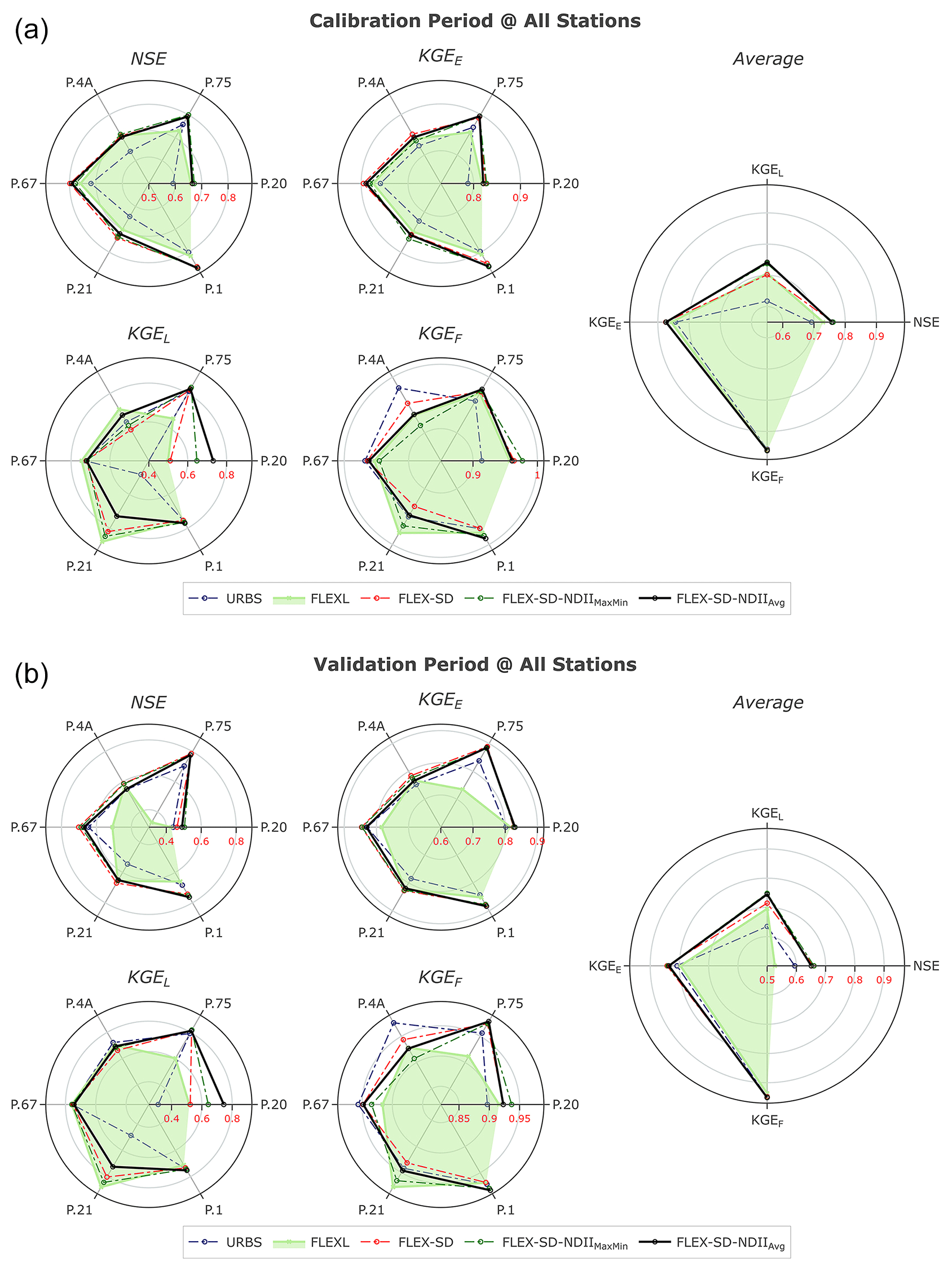
Figure 4 Comparison of the statistical indicators by (a) calibration and (b) validation at each station, using FLEXL and four semi-distributed models.

In conclusion, all developed FLEX-SD-based models can simulate runoff with similar accuracy or perform even better than the lumped model, FLEXL, and the established semi-distributed model, URBS.

5.1.2 Performance of semi-distributed models by calibration/validation at P.1

As previously mentioned, the performance of FLEXL at each gauging station provides a baseline comparison for the results of the semi-distributed models in the predictive mode. Over the calibration period (Fig. 5a), the FLEX-SD-based models produced similar accuracies (average NSE = 0.72–0.75), while URBS performed slightly worse (NSE = 0.68). This is comparable to, if not slightly better than, FLEXL (NSE = 0.73). However, in terms of the KGE_E indicator, FLEXL (KGE_E=0.86) performs notably better than the semi-distributed models (KGE_E=0.78–0.82). For the validation period (Fig. 5b), the FLEX-SD-based models (NSE = 0.67–0.70) and URBS (NSE = 0.65) performed notably better than FLEXL (NSE = 0.53).

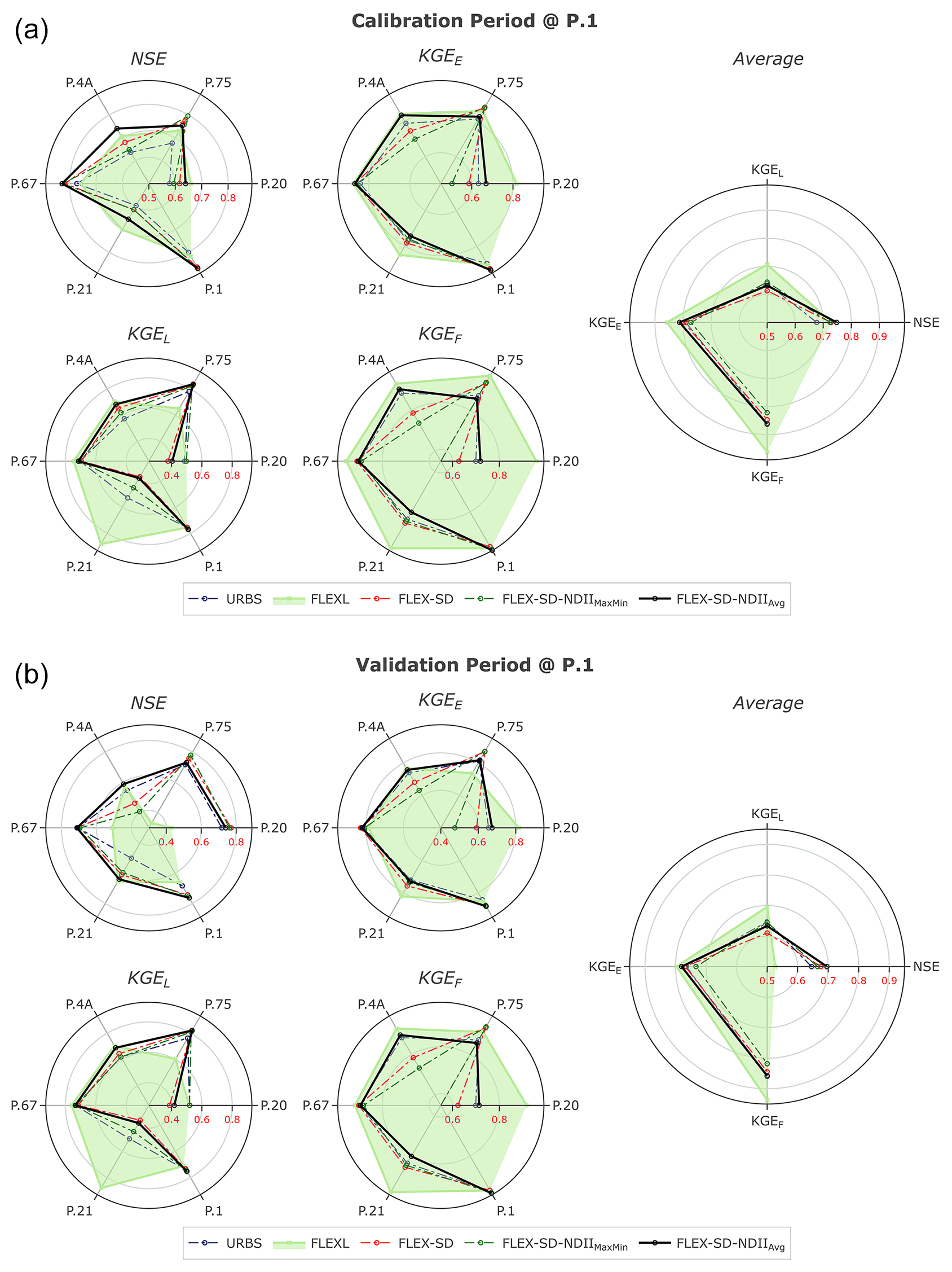
Figure 5 Comparison between the statistical indicators by calibration (a) and validation (b) at each station using FLEXL and by calibration and validation at P.1 using four semi-distributed models.

As shown in Fig. A1, the semi-distributed models are not capable of closing the water balance in four stations, except at the most downstream stations (P.67 and P.1). Additionally, the calibration/validation performed at all stations also closes the water balance better than achieved in predictive mode, although this may be due to over-fitting. Nonetheless, the fact that the validation mode of all semi-distributed models obtains more accurate results than the lumped and calibrated FLEXL model indicates a higher predictive capacity of the semi-distributed models.

Needless to say, issues such as flow regulation and water withdrawal pose challenges to these semi-distributed models. This is apparent at P.75, where outflows from Mae Ngat reservoir were potentially abstracted for agricultural demands but were unaccounted for, thereby causing notable overestimations of observed flows. This is reinforced in Fig. A3, which shows the lowest observed flows to be mostly below the modelled flows. P.4A also revealed overestimated flows, which drain a mountainous catchment with evergreen forest. In contrast, flow underestimations were seen in P.21 and P.20, which are intensively used catchments with rating problems (see Fig. 2). The lumped models are apparently not yet able to distinguish well between different landscapes. A landscape-based model, as suggested by Gharari et al. (2011) and Savenije (2010), could be the next step for improvement.

5.1.3 Discussion of model parameters

The model parameters used in FLEXL, FLEX-SD, and FLEX-SD-NDII_MaxMin and FLEX-SD-NDII_Avg are summarised in Table A1. The FLEX-SD-based models provide different values for TlagF (the time lag between storm and fast-runoff generation) and TlagS (the lag time of recharge from the root zone to the groundwater); the other parameters are kept the same as the calibrated values for P.1. Since TlagF and TlagS were designed to be related to the catchment area, the parameter values for each station are more reasonable compared to the values given by FLEXL. It can be noted that the values of TlagF obtained by FLEX-SD-NDII_Avg are much closer to the ones presented by FLEX-SD compared to the values obtained by FLEX-SD-NDII_MaxMin.

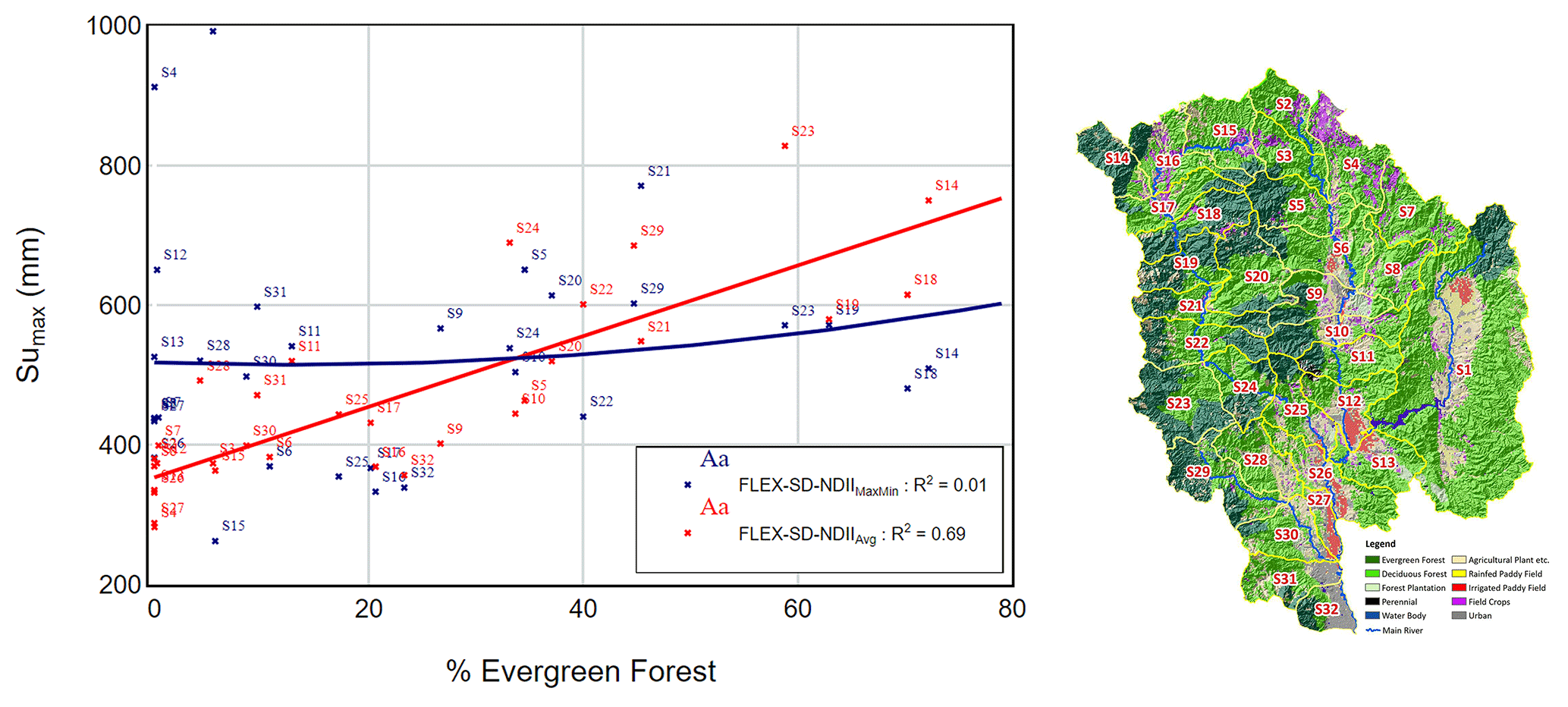
Figure 6 Relationships between the percentage of evergreen forest and modelled Sumax in 31 sub-catchments, as calibrated and validated by FLEX-SD-NDII_Avg and FLEX-SD-NDII_MaxMin. The topography of UPRB is presented alongside.

In general, FLEX-SD provides lower Sumax estimates than the other models, constraining evaporation in the dry season but compensating for this reduction with a smaller β value so as to limit excessive flood generation. Since these parameters jointly control Eq. (7), they can compensate for each other, leading to equifinality. If one of the parameters is constrained by additional information, as is the case here using the NDII, then this is no longer possible. The performance with respect to best-fit parameters may reduce in the process, but the model has gained realism and hence predictive power.

We see that the FLEXL-SD-NDII models show the highest realism (illustrated in Fig. A2) but not a very good performance in the sub-catchment P.20, although they are still better than the other semi-distributed models. P.20 remains a difficult sub-catchment to predict, due to its flow regulation and water consumption. Also, we see that adding constraints to model calibration does not always improve best-fit performance, as compared to free calibration, but that realism can be improved.

5.2 Relationship between Sumax and percentage of evergreen forests at the sub-catchment scale

The relationship between modelled Sumax values and the proportion of evergreen forests in each sub-catchment has been presented in Fig. 6. R² of 0.69 and 0.01 were yielded by FLEX-SD-NDII_Avg and FLEX-SD-NDII_MaxMin, respectively, indicating that Sumax values from the former model increase with greater vegetation coverage. With this unforeseen distinguishing power between sub-catchments of varying land use compositions, it is worth investigating the merit of implementing FLEX-SD-NDII_Avg in the ungauged basins. To further test the realism of the models, the outputs of the models were compared to observations of NDII and the global-scale SWI dataset for verification, as described in Sect. 5.3.

5.3 Uncertainty in runoff estimation using FLEX-SD, FLEX-SD-NDII_MaxMin, and FLEX-SD-NDII_Avg

Figure 7 displays the 2500 parameter sets selected to demonstrate the uncertainty (KGE_E, KGE_F, and KGE_L) at the six gauging stations. The results of all indicators are similar at P.67 and P.1. At Station P.75, KGE_L values are similar, while KGE_E and KGE_F provided by FLEX-SD-NDII_MaxMin are slightly higher than the others. At P.21, FLEX-SD performed marginally better than the others for all indicators. The most notable observations are at P.4A and P.20, where FLEX-SD-NDII_Avg is shown to outperform the others in terms of KGE_E and KGE_F. This is reinforced by the observed and calculated hydrographs in Fig. A4, where this model shows the narrowest uncertainty band at these stations. Moreover, the uncertainty bands in the flow duration curves of Fig. A5 show that FLEX-SD-NDII_Avg produced the narrowest bands at P.4A and P.21, but FLEX-SD showed the best performance at P.20 and P.67. In summary, all models show similar uncertainties; however, FLEX-SD-NDII_Avg reveals significantly better performance for upstream sub-catchments and not much difference for other areas compared to the other two models.

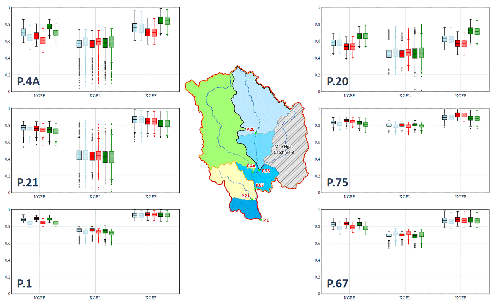
Figure 7 Comparison of box plots of the KGE_E, KGE_L, and KGE_F at six gauging stations provided by three FLEX-SD models using 5 % best-performing parameter sets. Full boxes indicate calibration and transparent boxes validation. Blue, red, and green indicate FLEX-SD, FLEX-SD-NDII_MaxMin, and FLEX-SD-NDII_Avg, respectively.

5.4 Relationship between the average root zone soil moisture storage (Su_i) and the average NDII and SWI

5.4.1 Su–NDII relationships

Figure 8 shows the R² and NSE during the wet and dry seasons for all six stations generated by three FLEX-SD models. Figure 8a shows that the time series of NDII correlates well with Su values during the dry season by giving an average R² value of 0.75–0.79. The average NSE values given by these models are 0.50-0.58, respectively. During the wet season, these correlations are lower (average R²=0.41–0.46; NSE = 0.44–0.49).

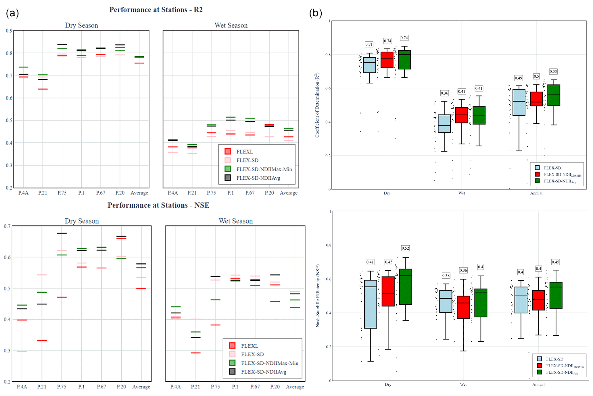
Figure 8 R² and NSE values from the exponential relationships between NDII values and simulated root zone moisture storage (Su) during the wet and dry seasons for six subbasins (a) and 31 sub-catchments (b) generated by three FLEX-SD models.

The same procedure was also carried out for all 31 sub-catchments and the results shown in Fig. 8b. During the dry season, the average R²=0.71–0.74, but FLEX-SD-NDII_Avg provided notably higher NSE (0.52) than FLEX-SD (0.41) and FLEX-SD-NDII_MaxMin (0.45). The relationships are significantly lower in the wet season (average R²=0.36–0.41; average NSE = 0.36–0.40). All in all, FLEX-SD-NDII_Avg provided higher R² and NSE than FLEX-SD-NDII_MaxMin in both seasons.

It is worth noting that FLEX-SD-NDII_Avg was able to differentiate the signatures in catchments of various soil moisture capacities. For a number of sub-catchments, particularly those with more evergreen forest (e.g. S14 = 72.2 %, S23 = 58.8 %, and S29 = 44.7 %), the estimates of Su from FLEX-SD-NDII_Avg provide notably higher NSE than others. Figure 9 presents the time series of simulated root zone moisture storage (Su), NDII, and SWI (discussed in following section) for a selection of contrasting sub-catchments. NDII signatures are well correlated with Su in sub-catchments with low percentages of evergreen forest (S4, S6, S9, S15, and S32). Low correlations were found in evergreen-forest-rich sub-catchments (S14, S23, and S29). The evergreen forest probably experiences less moisture stress compared to other land use land cover (LULC), so the situation NDII does not relate as well to simulated root zone soil moisture.

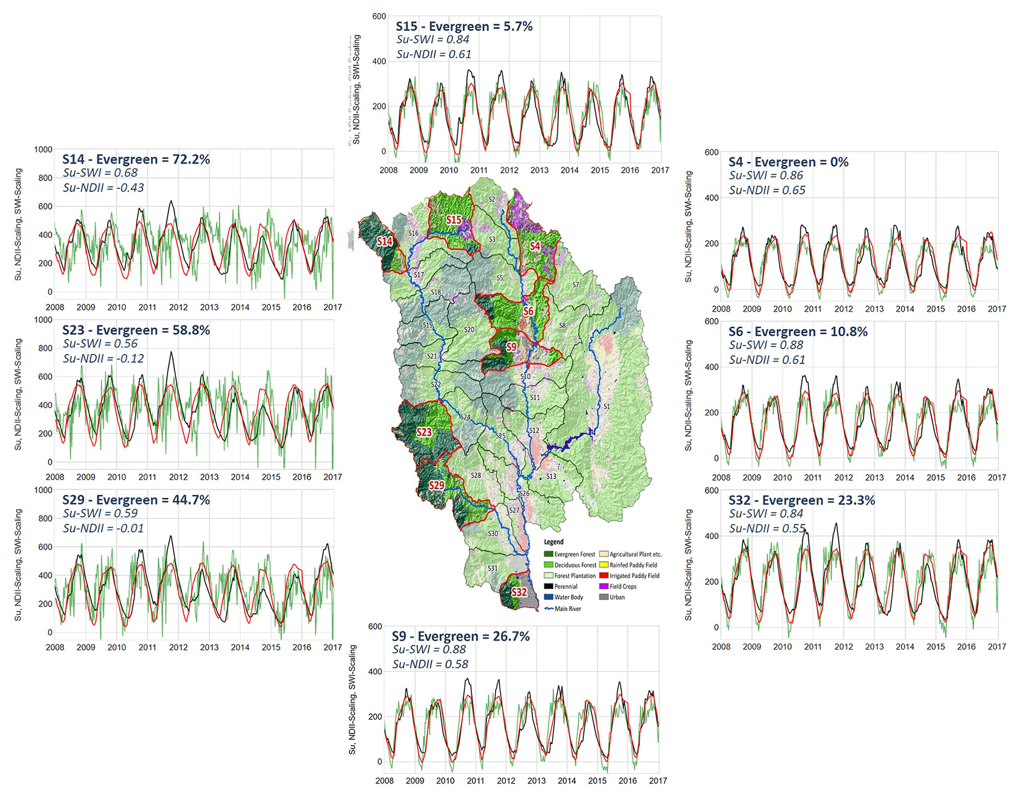
Figure 9 Comparison between simulated root zone moisture storage (Su; in black), NDII (in green), and SWI (in red) for eight sample sub-catchments with different percentages of evergreen forest.

5.4.2 Su–SWI40 relationships

Through testing all available characteristic time lengths (TLs) of SWI, the TL of 40 d produced the optimal Su–SWI relationship across the six gauging stations. This was thereby used for subsequent investigation and referred to as SWI40. Figure 10 shows the R² and NSE at all six stations simulated by the FLEX-SD-based models. Figure 10a shows that SWI40 correlates well with Su values during the dry season (R²=0.86–0.89 and NSE = 0.76–0.81). During the wet season, these correlations are of the same order of magnitude as in the dry season (R²=0.87–0.89 and NSE = 0.80–0.84). The results for all 31 sub-catchments are shown in Fig. 10b, which show average R² values of 0.86–0.87 and NSE of 0.78–0.79 during the dry season. During the wet season, R² values of 0.87 and NSE of 0.79–0.81 were yielded.

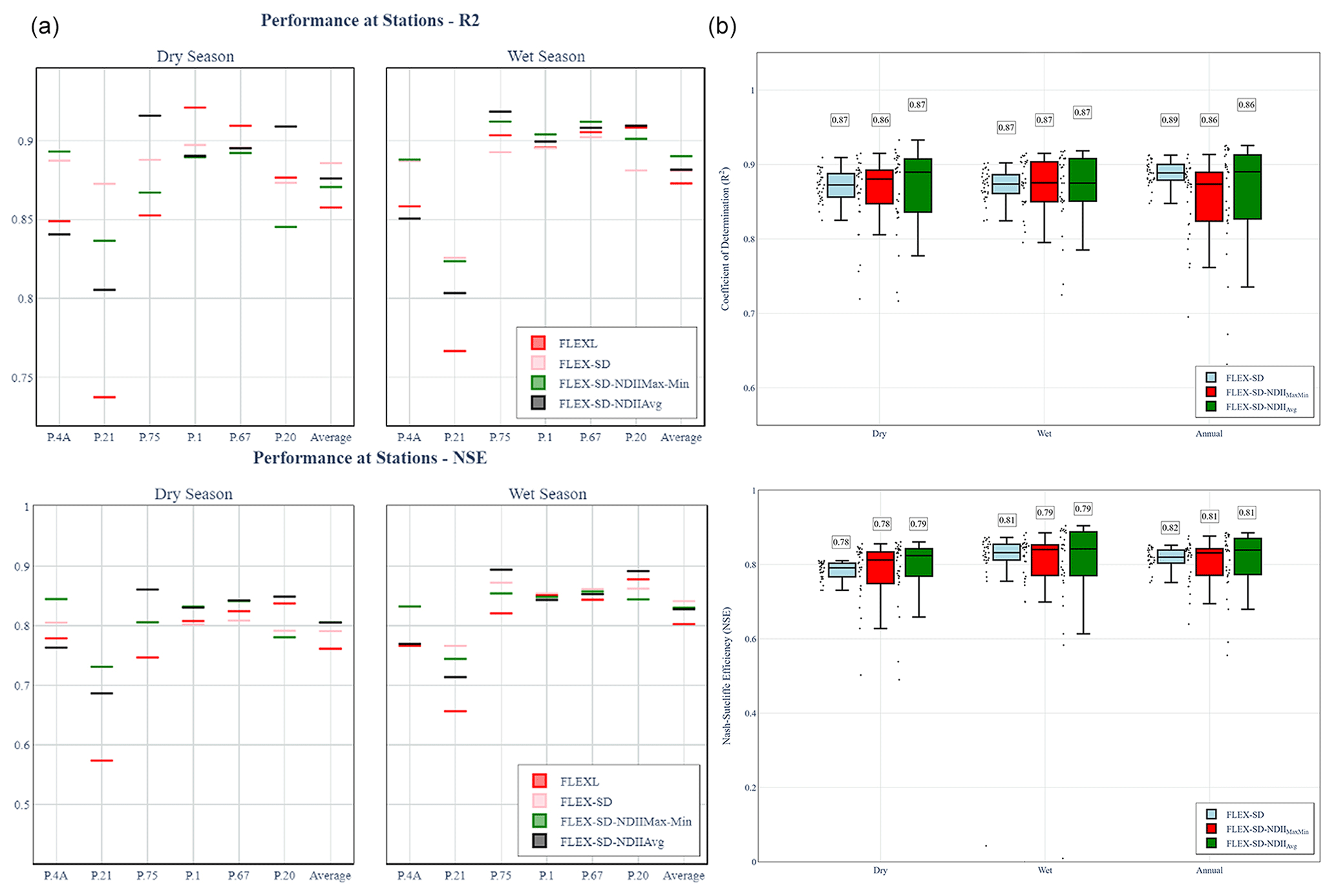
Figure 10 R² and NSE values from the exponential relationships between SWI40 and simulated root zone moisture storage (Su) during the wet and dry seasons for six subbasins (a) and 31 sub-catchments (b), as generated by three FLEX-SD models.

Despite the overall consistency in the average performance amongst these models and limited seasonality, it is evident that FLEX-SD-NDII_Avg shows the most variability across the 31 sub-catchments. In addition to the sensitivity of NDII to the proportion of evergreen forests, Fig. 9 also reveals the sensitivity of SWI40 to it. This is reflected in the notable time lag of the Su time series from SWI40 in the productive sub-catchments (e.g. S14, S23, and S29). This observation was not apparent with Su derived from FLEX-SD or FLEX-SD-NDII_MaxMin.

6 Discussion

Inspired by the significance of Sumax in governing the hydrological cycle, we investigated the utilisation of NDII to constrain our formulated FLEX-SD model with the objective of distributing the parameter of interest across the UPRB's 31 sub-catchments. The distribution of Sumax, particularly as achieved by FLEX-SD-NDII_Avg, helped produce better-informed runoff estimates for the gauged (especially for stations P.4A and P.20, which are densely forested areas) and ungauged sub-catchments than FLEX-SD, FLEX-SD-NDII_MaxMin, and URBS. The analysis of model uncertainties reinforces the improvements to flow estimation in ungauged sub-catchments. As explained below, this study has raised a few points worthy of discussion.

1. With the better representation of Su, the Su–NDII relationship yielded has become more informative about the underlying degree of aridity; that is, arid and productive sub-catchments exhibit greater differences than presented by FLEX-SD and FLEX-SD-NDII_MaxMin. The increased variation challenges the preconception from the study by Sriwongsitanon et al. (2016) that NDII is a suitable proxy for RZSM dynamics in the dry season, as it was hereby shown to barely correspond with Su_i in evergreen forests under any circumstances.

2. Upon testing the accuracy of derived Su_i against SWI, we realise the potential of implementing SWI to indicate moisture states of river basins. However, we should be reminded of its simplicity, such as using a single parameter, T, to emulate RZSM signatures. Furthermore, the model lacks the ability to account for the effects of local characteristics (e.g. LULC), which likely explains the variable Su–SWI correlation across the 31 sub-catchments. Nonetheless, in future work, we are convinced that appropriately manipulating the T parameter to specific catchments, instead of using a T value of 40 d to represent the RZSM characteristics of the entire catchment as done in this study, could widen the potential of implementing SWI to indicate moisture states in river basins of contrasting characteristics.

3. It is worth noting the increased variability in Su–SWI across the 31 sub-catchments (as seen in Fig. 10), in spite of the systematic increase in Su–NDII, which, counterintuitively, could be attributed to the improved realism of the FLEX-SD-NDII_Avg. That is, by using NDII to distribute Sumax, and thereby improving accuracy of estimated runoff, this accounts for the greater variability in Su signatures across the 31 sub-catchments than was produced by FLEX-SD.

7 Conclusion

Most lumped rainfall–runoff models are controlled by a gauging station at the outfall on which it is calibrated. Runoff estimation at any location upstream requires indirect approaches, such as model parameter transfer from gauged stations to ungauged locations, or applying relationships between model parameters and catchment characteristics to the ungauged locations. By using any of these approaches, the uncertainty in runoff estimation for ungauged catchments is unavoidable. A semi-distributed hydrological model could offer a better alternative. Besides considering lag times and flood routing (as in FLEX-SD), it has been shown that it is required to account for the spatial variation in the moisture-holding capacity of the root zone. Therefore, the model was constrained by using NDII patterns (particularly average NDII, so as to produce the FLEX-SD-NDII_Avg) as a proxy for the spatial variation in root zone moisture leading to distributed Sumax values among sub-catchments. The model parameters provided by the semi-distributed FLEX models are more realistic compared to the original FLEXL, since they are distributed according to catchment characteristics comprising catchment area, reach length, and the NDII.

With the inclusion of NDII, the estimated catchment-scale root zone soil moisture (Su_i) has been shown to be increasingly sensitive to the underlying degree of aridity, which is arguably more representative of the hydrological responses across heterogeneous sub-catchments. Such knowledge should be used in further studies to explore the opportunities of implementing the model-based SWI to estimate soil moisture in different land use land cover.

Appendix A

Table A1 Model parameters of FLEXL (calibrated at all stations) and FLEX-SD and FLEX-SD-NDII (calibrated only at P.1).

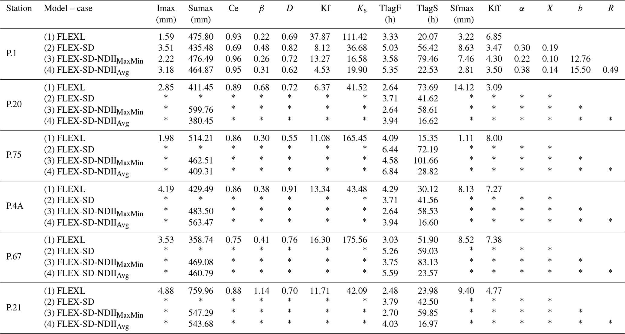
Note that the asterisk^* indicates the same parameter values as P.1 for FLEX-SD and FLEX-SD-NDII.

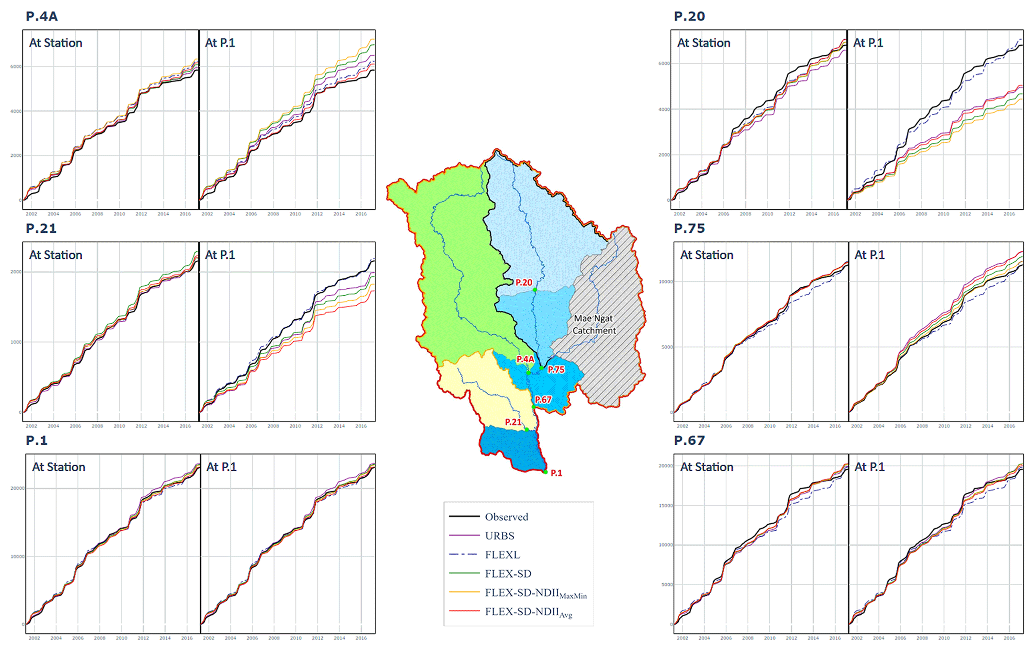
Figure A1 Accumulated simulated and observed runoff (units in MCM) of all models produced by calibration and validation at (1) each station (At Station) and (2) at P.1. Note that FLEXL is the only lumped model and was thereby only calibrated at each station.

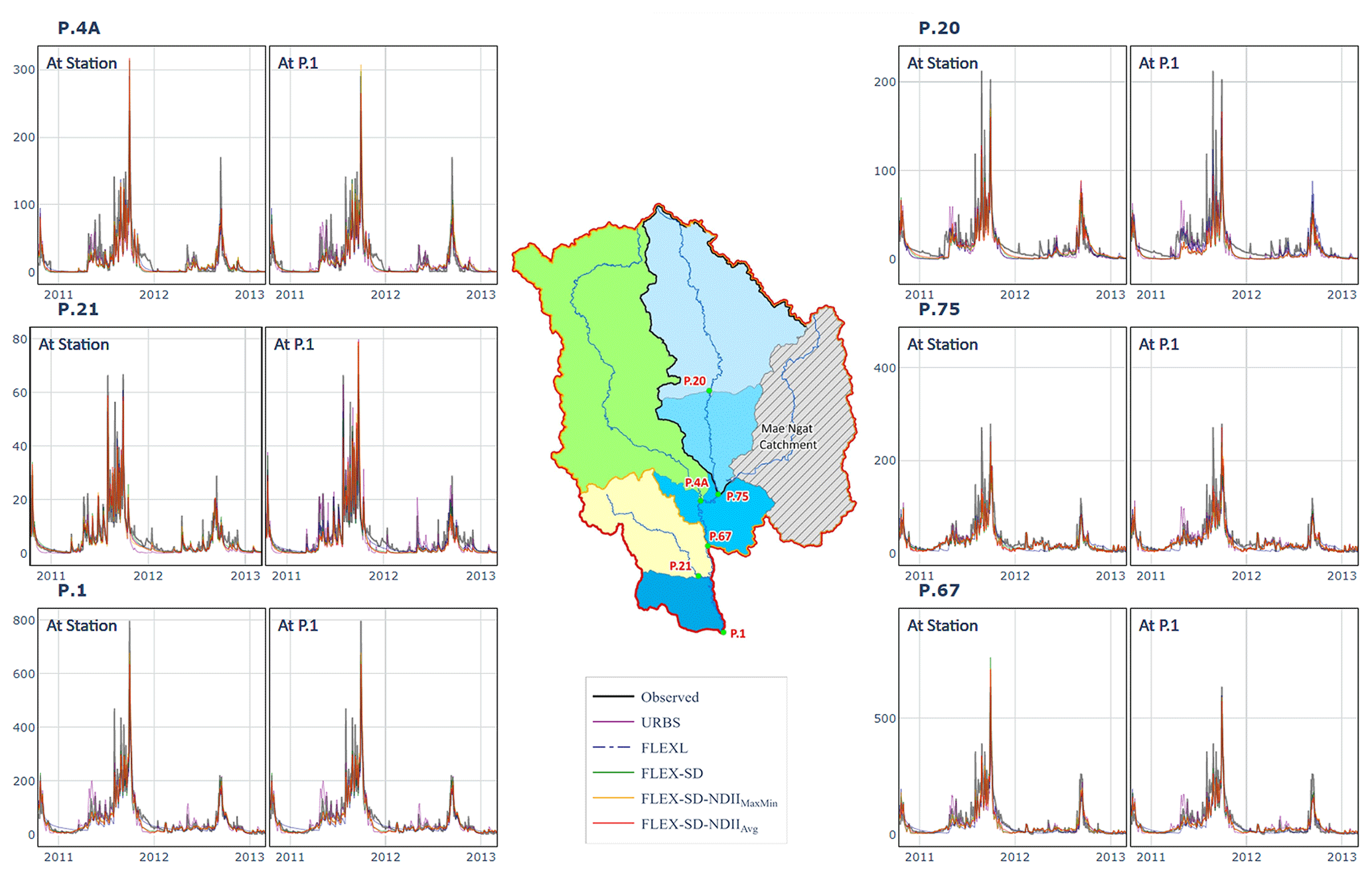
Figure A2 Hydrographs of simulated and observed runoff (units in cubic metres per second) of all models at all stations produced by calibration and validation at (1) each station (At Station) and (2) at P.1. Note that FLEXL is the only lumped model and was thereby only calibrated at each station.

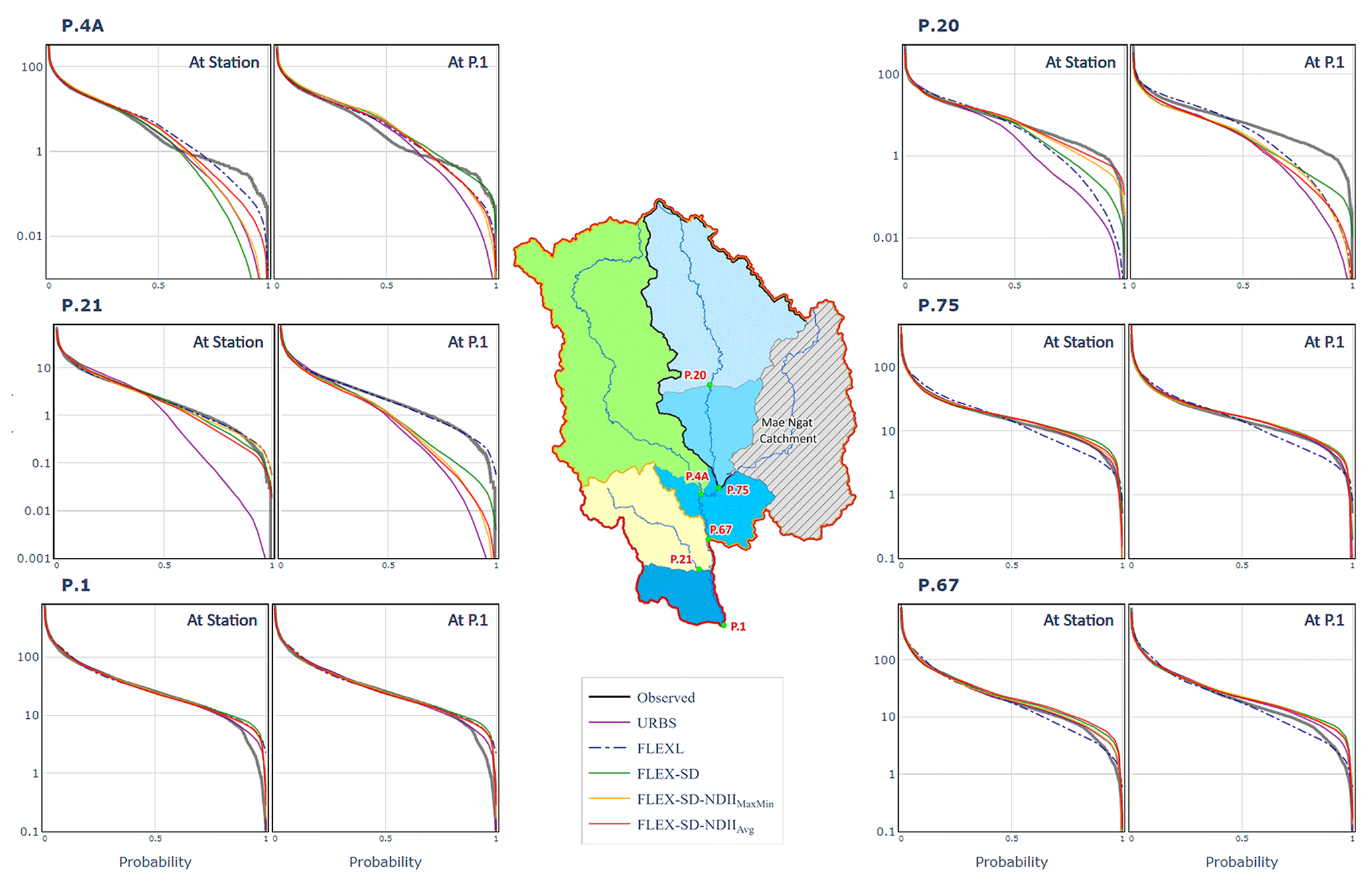
Figure A3 Flow duration curves of simulated and observed runoff of all models at all stations produced by calibration and validation at (1) each station (At Station) and (2) at P.1. Note that FLEXL is the only lumped model and was thereby only calibrated at each station.

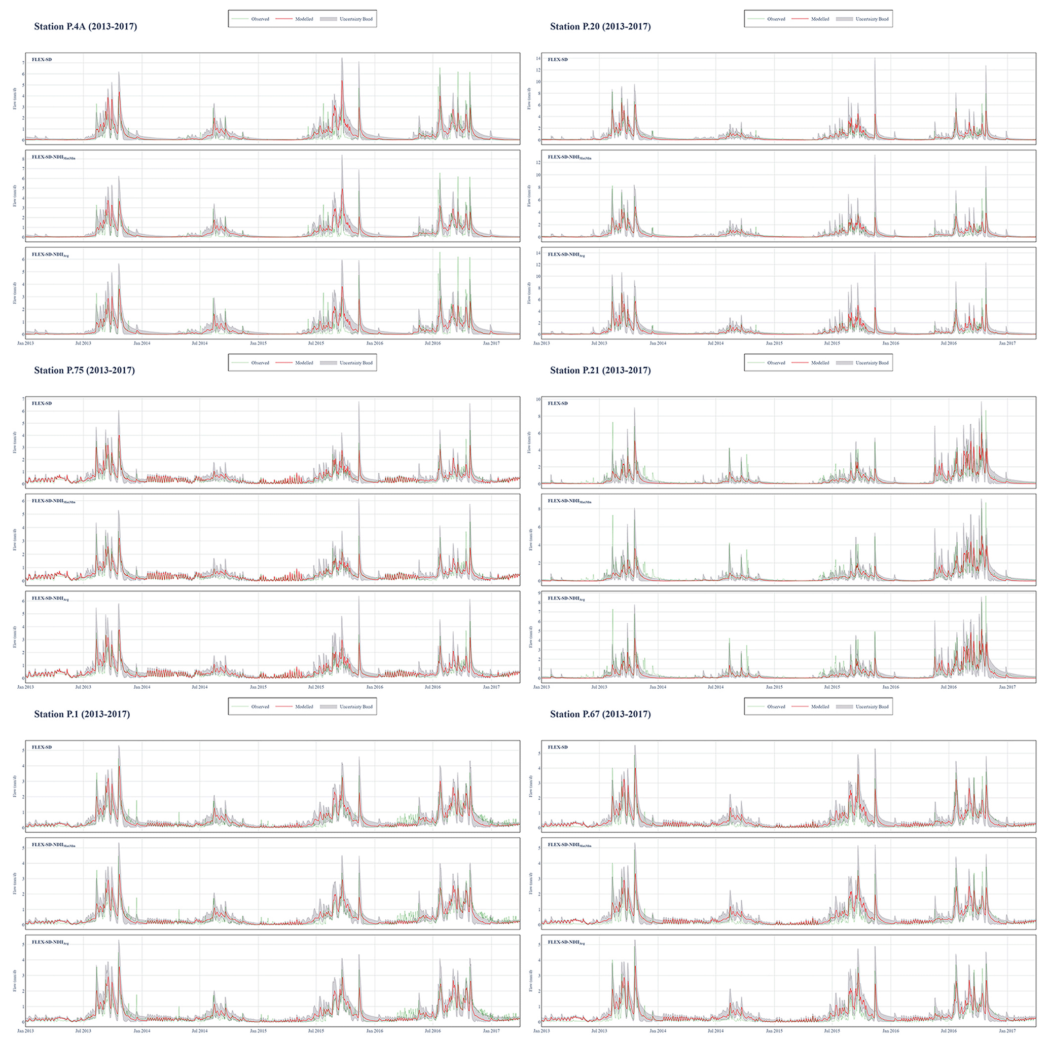
Figure A4 Comparison of the observed and calculated hydrographs at six stations acquired from the 5 % best-performing parameter combinations generated by three FLEX-SD models.

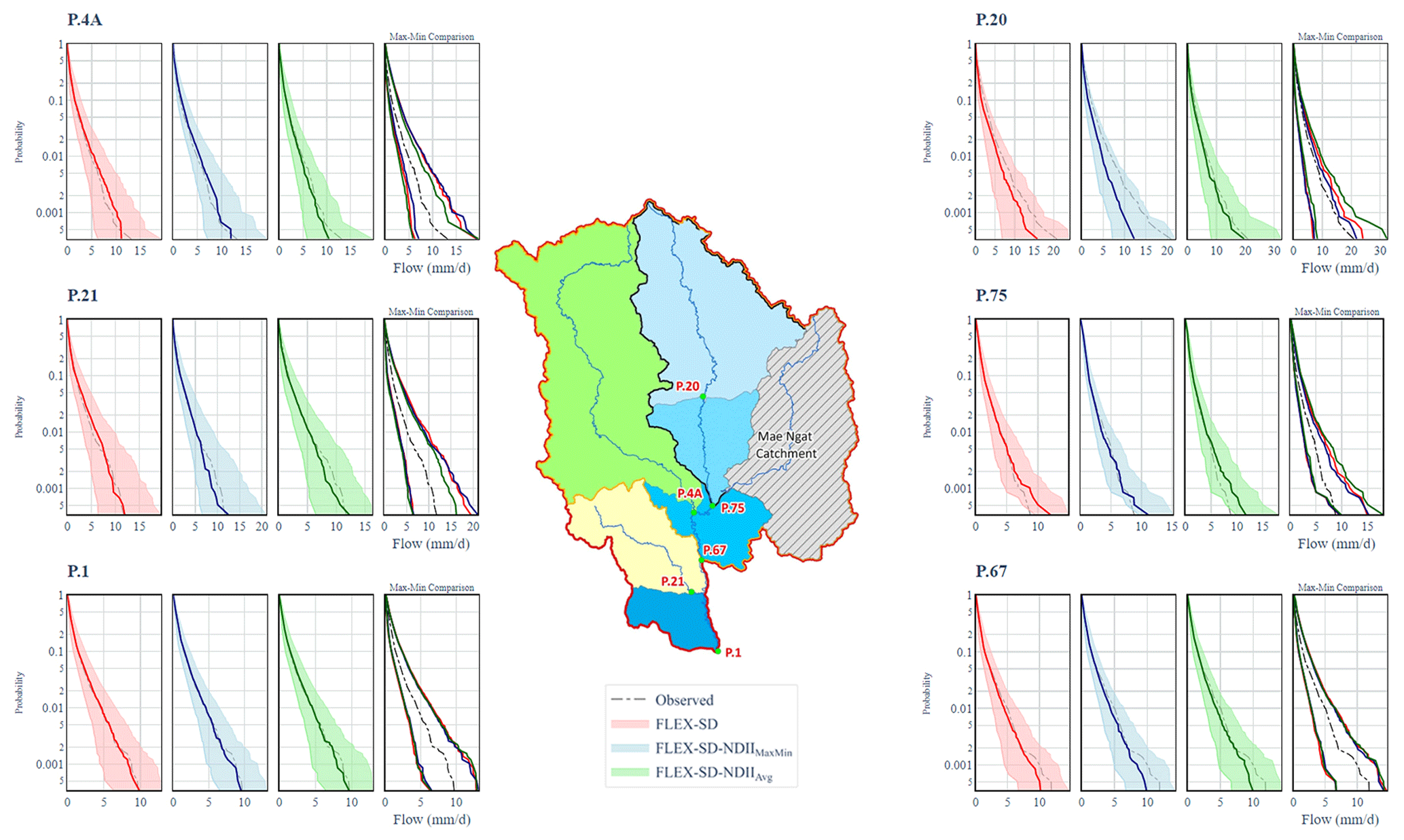
Figure A5 Comparison of the observed and calculated flow duration curves at six stations acquired from the 5 % best-performing parameter combinations generated by three FLEX-SD models.