the Creative Commons Attribution 4.0 License.
the Creative Commons Attribution 4.0 License.
 | 26 May 2023
An optimized long short-term memory (LSTM)-based approach applied to early warning and forecasting of ponding in the urban drainage system
Wen Zhu
Tao Tao
Hexiang Yan
Jieru Yan
Jiaying Wang
Shuping Li
Kunlun Xin
In this study, we propose an optimized long short-term memory (LSTM)-based approach which is applied to early warning and forecasting of ponding in the urban drainage system. This approach can quickly identify and locate ponding with relatively high accuracy. Based on the approach, a model is developed, which is constructed by two tandem processes and utilizes a multi-task learning mechanism. The superiority of the developed model was demonstrated by comparing with two widely used neural networks (LSTM and convolutional neural networks). Then, the model was further revised with the available monitoring data in the study area to achieve higher accuracy. We also discussed how the number of selected monitoring points influenced the performance of the corrected model. In this study, over 15 000 designed rainfall events were used for model training, covering various extreme weather conditions.
- Article
(8214 KB) - Full-text XML
- BibTeX
- EndNote


The intensity and frequency of urban floods are growing as a result of the increased frequency of extreme weather, rapid urbanization, and climate change (Hossain Anni et al., 2020; Guo et al., 2021; Huong and Pathirana, 2013). It is becoming increasingly clear that urban floods significantly impact city management and endanger the safety of peoples' lives and the stability of various property types. The ability to reliably characterize and forecast urban floods and generate high-precision flood risk maps has become critical in flood mitigation and decision-making.
The most common approach to simulating urban floods is to develop a hydrodynamic model (i.e., storm-inundation simulation), which utilizes a collected topographic map, information on the pipe network, historical rainfall data, monitoring data, and other information on the study area (Jamali et al., 2018; Aryal et al., 2020; Balstrøm and Crawford, 2018; Tian et al., 2019). However, a realistic hydrodynamic model for continuous simulation requires vast data, such as comprehensive information on topography, infiltration conditions, and sewage system data (including exact locations, depths, and diameters of sewage pipes). However, the above data are difficult to obtain, especially in metropolitan areas (Rahman et al., 2002; Kuczera et al., 2006). Furthermore, the calculation in a storm-inundation simulation is sophisticated and often computationally intensive, which takes a long time to execute. The most detailed representation of the storm-inundation simulation is the 1D–2D model (Djordjević et al., 1999, 2005), which summarizes the dynamic interaction between the flow that enters the underground drainage network and the overloaded flow that spreads to the surface flow network during high-intensity rainfall. Representatives of such a model include XPSWMM, TUFLOW, and MIKE FLOOD (Leandro and Martins, 2016; Teng et al., 2017; Zhang and Pan, 2014).
The lack of underlying information has hampered the continuous development of hydrodynamic models in urban flood forecasting. As a result, deep learning has emerged as another viable forecasting tool. Deep learning is a particular machine-learning technique that leverages neural networks to learn nonlinear relationships from a dataset (Mudashiru et al., 2021; Sit et al., 2020; Shen, 2018; Moy De Vitry et al., 2019). It can compensate for data scarcity by training on a large designed dataset. Unlike traditional hydrodynamic models, deep learning does not require any assumptions on the physical processes behind it.
However, there are opportunities to further the application of deep learning in urban flood forecasting. First, the training dataset needs to be enriched to reflect the superiority of the approach. Many studies in urban flood forecasting only use a small number of samples to develop the deep learning models. For example, Cai and Yu (2022) used 25 historical floods for forecasting. Abou Rjeily et al. (2017) used only 10 rainfall events for training and verification, which was insufficient to reflect the characteristics of rainfall distribution. Second, due to the high cost of monitoring equipment, researchers usually have to rely on unvalidated simulations produced from hydrodynamic models. For example, Chiang et al. (2010) used synthetic data from the SWMM model as the target values to train the recurrent neural network (RNN) and then compared the predictions with simulation results to evaluate the model accuracy in estimating water levels at ungauged locations. Third, some studies have focused on building more complex deep learning architectures to improve model performance. Examples include but are not limited to the automatic encoder (Bai et al., 2019), the encoder–decoder (Kao et al., 2020), and customized layers based on long short-term memory (LSTM; Sit et al., 2020; Kratzert et al., 2019a, b). For example, an encoder–decoder LSTM has been proposed for runoff forecasting up to 6 and 24 h ahead (Xiang et al., 2020; Kao et al., 2020). Nevertheless, the urban flooding forecasting tasks with multiple time steps are mainly based on the precipitation forecast hours in advance, which is not available in this paper. Because of the short duration of rainfall, the real-time data volume is not enough to support the hours-ahead prediction.
In this study, we propose an optimized LSTM-based approach for the early warning and forecasting of ponding in urban drainage system. This approach can quickly identify and locate ponding with relatively high accuracy. The model is constructed by two tandem processes and introduces a multi-task learning mechanism. The evaluation results of the model were compared with those of two widely used neural networks, i.e., LSTM and CNN (convolutional neural network). The model was further revised with monitoring data in the study area to improve the emulation performance. We also discussed the influence of the number of monitoring points selected on the model performance. Over 15 000 designed rainfall events were used for model training, covering various extreme weather conditions.
The rest of the paper is organized as follows: Sect. 2 introduces the methodology used to develop the LSTM-based modeling framework in addition to the experimental setup and application of the model. Section 3 presents the results of the model. Section 4 presents the discussion, and Sect. 5 concludes this paper by drawing brief conclusions.
2.1 LSTM-based model
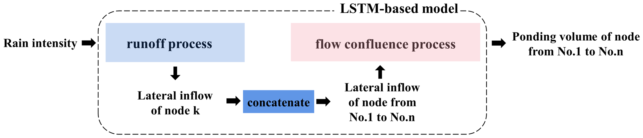
Like a hydrodynamic model, which is generally composed of two processes, namely the runoff process and flow confluence process, the LSTM-based model proposed in this study is also constructed with two stages. Figure 1 illustrates the model architecture from input (i.e., rain intensity) to output (i.e., ponding volume of each node).
The two processes are in tandem; the inputs of the flow confluence process are inherited and concatenated from the outputs of all nodes in the runoff process. However, during the training process, the two processes are trained separately without mutual interference, as the inputs and outputs of both processes are produced from a hydrodynamic model.
2.1.1 Runoff process
With a general understanding of a hydrodynamic model, the runoff process involves surface runoff and infiltration, while the most important influential factor is rainfall. As a mass rainfall curve can reflect the characteristics of a specific rainfall process, it can be directly used as the input of a neural network. The output of the neural network (i.e., lateral inflows at each node) reflects the hydraulic state in the runoff process.
Figure 2 illustrates the training, validation, and testing procedures in the runoff process. As shown in Fig. 2, a training set with two time series of data is fed into the neural network, thus giving the rainfall intensity and lateral inflow at each node. At each epoch, four indicators are used to evaluate the consistency between the predicted lateral inflows and the simulation from the hydrodynamic model. If the model converges, the network is further evaluated on the test set. Otherwise, the next training epoch is started.
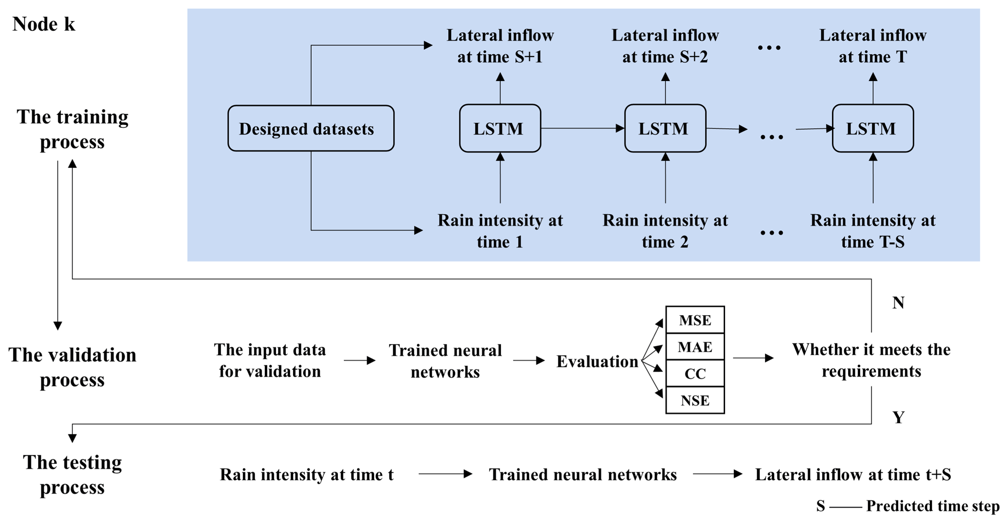
Figure 2The training, validation, and testing procedures used when developing the LSTM-based runoff emulator (MAE – mean absolute error; MSE – mean squared error; CC – correlation coefficient; NSE – Nash–Sutcliffe efficiency coefficient).
2.1.2 Flow confluence process
The flow confluence process is set up in the same manner as the simulation process of a hydrodynamic model (e.g., the SWMM model). If we compare the urban drainage system to a black box, then only the lateral inflows at each node and outflows from the outlets enter and leave the system, respectively (Archetti et al., 2011). If a free-outflow condition is considered, namely the hydraulic state behind the outlets has little influence on the interior of the system, then the inputs of the flow confluence process are only the lateral inflows at each node. Figure 3 illustrates the details of the network architecture in the flow confluence process.
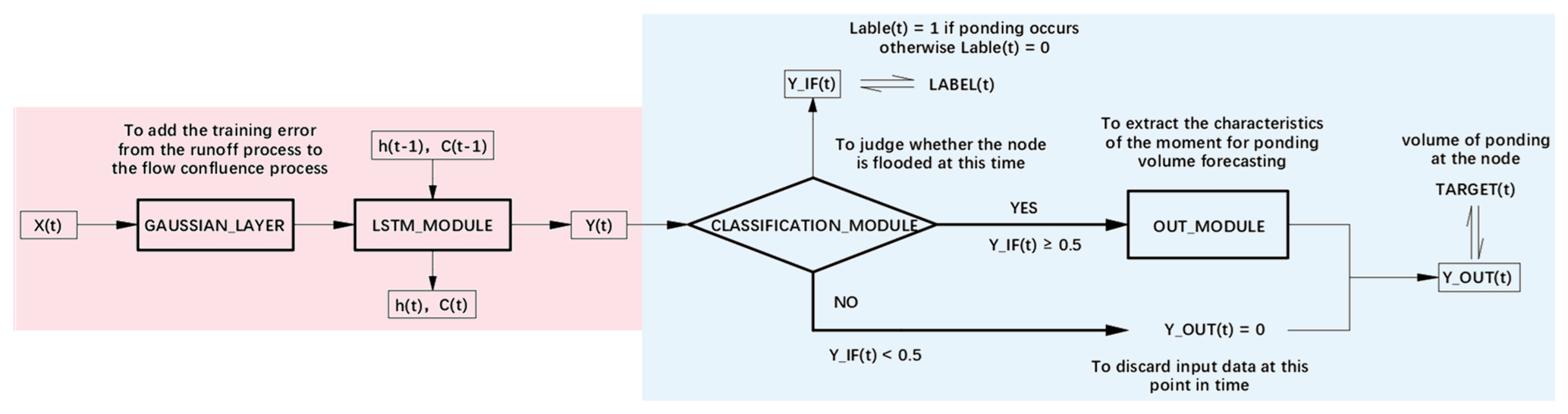
As illustrated in the pink block in Fig. 3, a Gaussian layer is added after the input layer in the flow confluence process during training. The Gaussian layer serves as a filter to compensate for the inaccuracy of the prediction (by the hydrodynamic model) in the runoff process. The model is trained to minimize the differences between the predictions (from the neural network; i.e., the output from the runoff process) and the simulations (from the hydrodynamic model). Then (as illustrated in the blue block in Fig. 3), a classification layer is added after the outputs of the LSTM module to judge whether ponding occurs at the time step. Only when ponding occurs at the time step can the output of the LSTM module enter the “OUT_MODULE” to continue with the learning. Otherwise, the output of the LSTM module at this time step is discarded. In this way, the interference of the time points without ponding on the ponding volume forecasting is eliminated to a great extent. The higher the classification accuracy, the more accurate the prediction of ponding volume will be. Moreover, the multi-task learning has a hard parameter-sharing mechanism, which effectively alleviates the overfitting of the model. The parameters in the “LSTM_MODULE” (including the parameters of the LSTM layers, batch normalization layers, activation functions, etc.) are shared by the “CLASSIFICATION_MODULE” and “OUT_MODULE”.
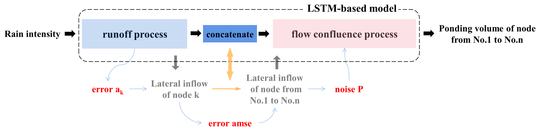
Figure 4The error transmission during training from the runoff process to the flow confluence process.
2.2 Error transmission
Figure 4 illustrates how the training error in the neural network propagates from the runoff process to the flow confluence process during training. Noise P () is added to the lateral inflows before feeding the data into the neural network in the flow confluence process in order to avoid the interference caused by the training error in the runoff process and also to alleviate the overfitting of the neural network. The magnitude of noise P can be determined as follows:
-
The mean squared error (MSE) is used to characterize the training error in the runoff process, where the error at node K can be computed by the following:
where T represents the duration of event j (in min), S represents the number of events in the training data, represents the simulated lateral inflow at node K at the ith time step in the jth rainfall event (in L s−1), and Xij represents the output of the runoff process at node K at the ith time step in the jth sample event (in L s−1).
-
Then the average mean squared error in all nodes is computed by the following:
where N represents the number of nodes.
-
Then amse is converted into the noise percentage ε, with the mean value of the predicted lateral inflows at all nodes in the training set, by the following:
where PS represents signal power, and PN represents noise power.
-
Finally, noise P is added to the inputs (X) in the flow confluence process during the training process. In other words, a set of random numbers G is generated with the length of X, using the pseudorandom number generator, where G obeys a normal distribution (); i.e., , where p is computed by the following:
2.3 Model correction system
The LSTM-based model is built based on the simulation results of a relatively accurate hydrodynamic model. However, the differences between the simulation from the hydrodynamic model at the monitoring points and the obtained monitoring data always exist during the operation of the pipe network, which leads to a discrepancy between the predicted results from the proposed LSTM-based model and the actual situation. Thus, it is necessary to correct the model using the measured level and flow data at the monitoring points. Moreover, how to revise the model properly using the available data is also one of the focuses of this study. Figure 5 describes the model correction process using the measured rainfall data, depths and flows at the monitoring points, and ponding data at any node. Specifically, the LSTM-based model is corrected using the following two steps:
-
The runoff process is corrected with the measured rain, level, and flow data by referring to the transfer learning. Transfer learning is mainly used to transfer the knowledge of one domain (source domain) to another domain (target domain), such that the target domain can achieve better learning effects (Pan and Yang, 2010).
-
The flow confluence process is corrected using the updated lateral inflows of all concatenated nodes and the measured ponding volume.
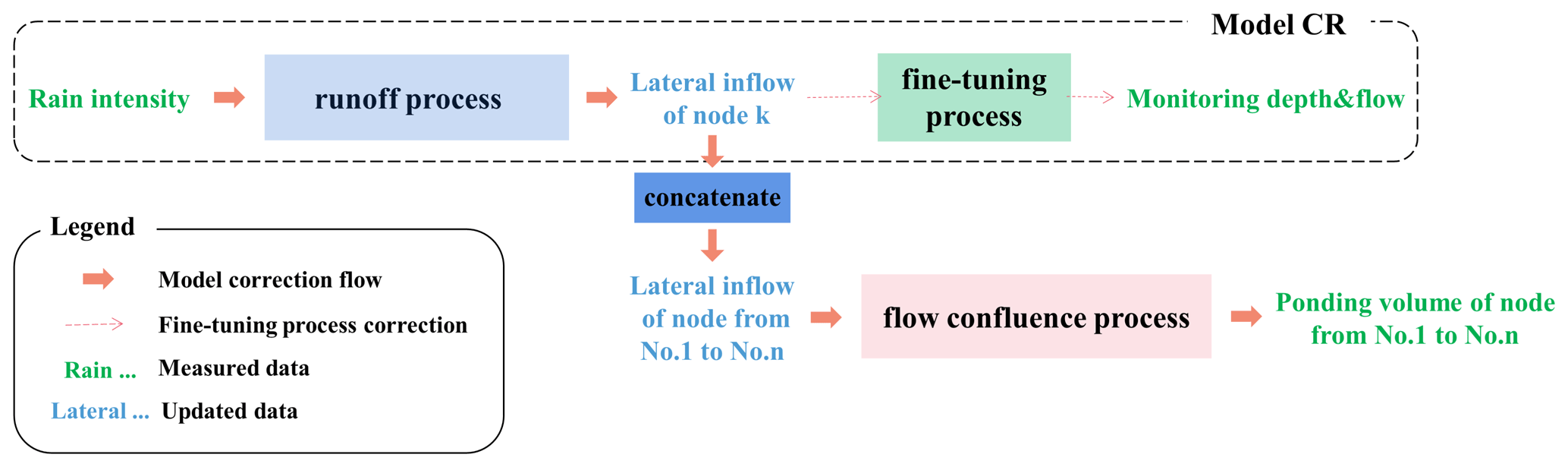
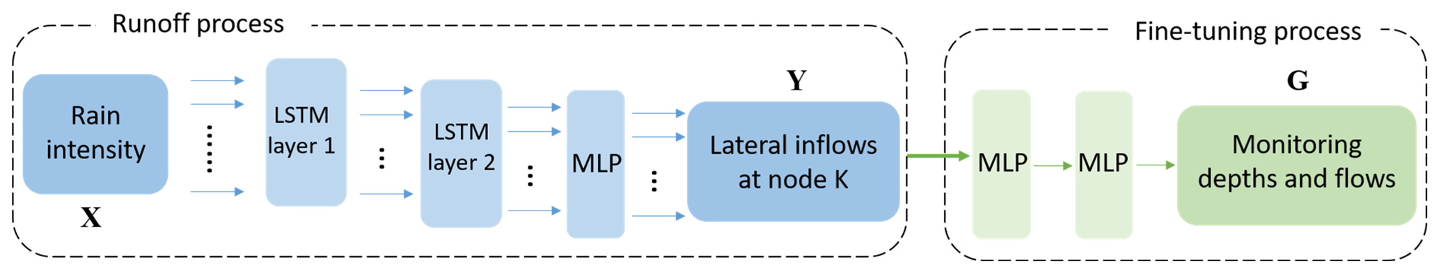
Figure 6 shows the schematic of model CR (correction of the runoff process). It migrates the network structure of the runoff process from rain data (X) to lateral inflows (Y) to the input–output connection between X and monitoring data (G). Then, multiple fully connected layers are added after the output layer of Y. Model CR is designed to update the runoff process in the primary LSTM-based model. The correction has two steps, namely training and updating. First, model CR is trained based on a pretrained mapping from X to Y (as shown in Sect. 2.1.1) with constructed rain data, a simulated level, and flow data. Then, it is updated on pairs of measured rain data, monitored water depths, and flows.
2.4 Case study
2.4.1 Study area
The LSTM-based model trains nodes in the pipe network one by one. Namely N submodels with the same architecture are generated, where N is the number of nodes in the system. In both the runoff process and flow confluence process, these submodels are trained separately. Due to this structural characteristic, the size of the case area does not limit the model's performance. Regarding the model structure, the output of the runoff process is the lateral inflow at a single node. Likewise, the output of the flow confluence process is the ponding volume at a single node. Regardless of the size of the pipe network, the output of the model is at each node. However, a large-scale pipe network with lots of nodes will significantly increase the time spent training the model and also require extra processing power.
To verify the feasibility of the modeling framework above, a small-scale case area JD, a residential district in S city, is selected as the study area. Figure 7a shows the elevation map of the study area. There are 32 residential buildings in the district, with a total area of 6.128 hm2. The study area is separated from the municipal roads by walls, with three entrances on the community's northern, eastern, and western sides. Rain pipes in the study area are circular pipes with 200, 300, 400, 500, or 600 mm in diameter (mostly 300 mm). The total length of this pipe network is 5.5 km. The network contains 336 nodes and 340 pipes and is connected to the municipal pipe networks through four outlets, as denoted by the green triangle in Fig. 7b. There are 15 level gauges and 3 flowmeters in the current pipe network. The layout of monitoring points is also shown in Fig. 7b.
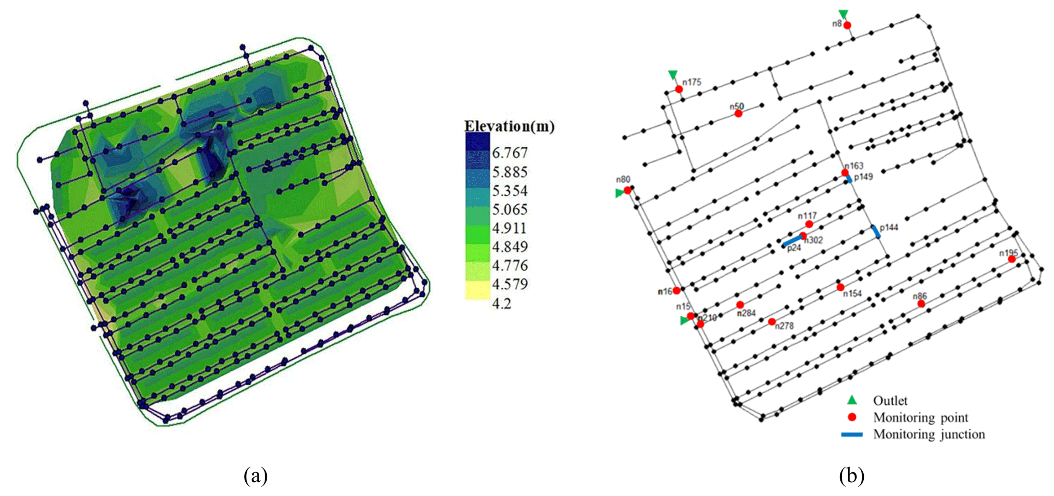
Figure 7Study area, JD, which is a residential district. (a) The elevation map and stormwater system in the case area. (b) The layout of the monitoring points in the case area.
2.4.2 Rainfall data
The rainstorm intensity for S city is designed using Eq. (5), which is obtained according to a universal design storm pattern proposed by Keifer and Chu (1957). The storm pattern is broadly used both at home and abroad. The generated storms are usually extreme enough to reflect the state of the pipe networks under the most unfavorable conditions (Skougaard Kaspersen et al., 2017).
where q is the rainstorm intensity (in L s−1 hm−2), P is the reappearing rainfall period (in a(a)), t is the duration of rainfall (in min), and A, C, b, and n are parameters of the rainstorm intensity design formula.
The rainstorm intensity before or after the peak is determined using Eq. (6).
where tb and ta are the times before and after the peak (in min), respectively, and r is the rainfall peak coefficient.
Then single-peak rainfall scenarios were constructed unevenly by using different rainfall reappearing periods (P) ranging from 0.5 to 100 a, a peak coefficient (r) ranging from 0.1 to 0.9, and a duration (T) ranging from 60 to 360 min.
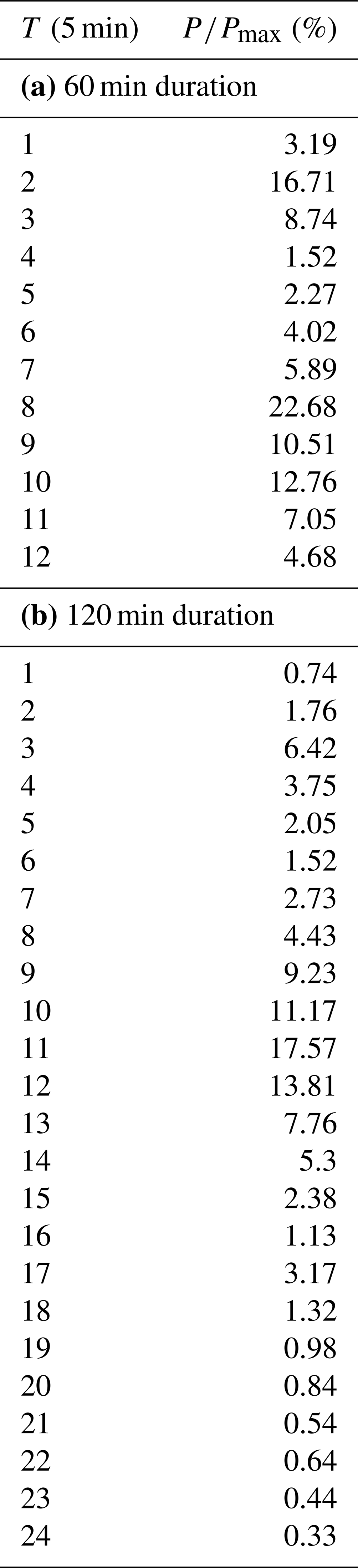
In addition to single-peak rainfall scenarios, we also considered bimodal rainfall scenarios. According to the historical bimodal rainfall data in S city, the rainfall peaks corresponding to the bimodal design storm pattern with the duration from 60 to 360 min could be computed by Pilgrim and Cordery (1975). Pilgrim and Cordery (1975) present a method to count the historical rainfall data and deduce the rainstorm pattern from it.
Table 1 shows the bimodal design storm patterns with 60 and 120 min duration time, respectively, where represents the distribution of rainfall intensity over time (with a 5 min unit period). Then, double-peak rainfall scenarios were constructed according to Table 1 using reappearing periods ranging from 0.5 to 100 a.
The produced single-/double-peak rainfall data were then added with Gaussian white noise (produced according to the procedures described in Sect. 2.2) to ensure that the obtained dataset contains enough extreme conditions. Take the rainfall with a return period of 5 a as an example. Figure 8 shows the effect of adding noise, where panel (1) shows the randomly generated Gaussian white noise over the duration, panel (2) shows the distribution of the reordered white noise, and panel (3) magnifies the part circled in panel (2). Panels (4)–(6) show the design rainfalls after adding 30 %, 50 %, and 70 % white noise, respectively. Specifically, we have limited the noises near the rainfall peak; i.e., only negative noises are allowed there.
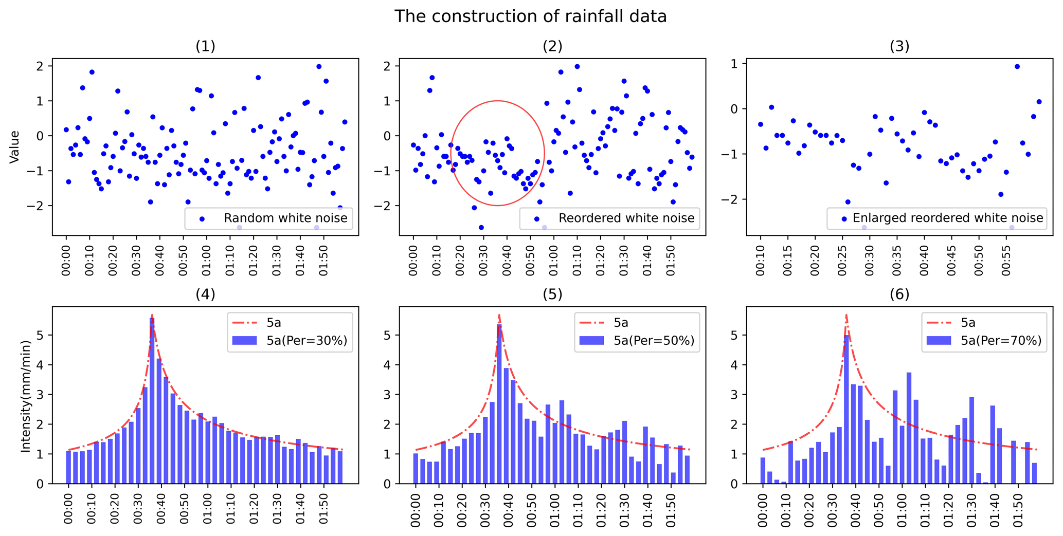
In this study, the noise percentages went from 0 % to 100 % in increments of 10 % to blur the characteristics of the design storm pattern and intensify the extreme conditions. The synthetic dataset contained a total of 16 960 rainfall events. The ratios of the training, validation, and test sets were 80 %, 10 %, and 10 %, respectively.
In general, a small training set normally leads to a poor approximation effect. Thus, a convergence test was performed to evaluate the data requirement for the proposed LSTM-based model to obtain the desired approximation effect. The model performances using different sizes of training data were compared, as shown in Fig. 9. When the data size was reduced to two-thirds of the origin volume, then the model performance fell down to 90 % of the original. Moreover, if the data size was halved, then less than 80 % of the origin model performance remained.

Figure 9The learning curve which describes the relationship between model performance and data volume.
2.4.3 Simulated and measured data
A hydrodynamic model was established for the case pipe network. The simulation results (i.e., the lateral inflows and the volume of ponding at each node, in addition to the level and flow data at the monitoring points) were obtained using the constructed rainfall events described in Sect. 2.4.2. In the simulation process, we considered a uniform rainfall distribution in space. A simplified representation of the sewer system and a constant, uniform infiltration rate in the green area were also considered for runoff computation (Löwe et al., 2021). Meanwhile, we did not consider the two-dimensional surface overflow.
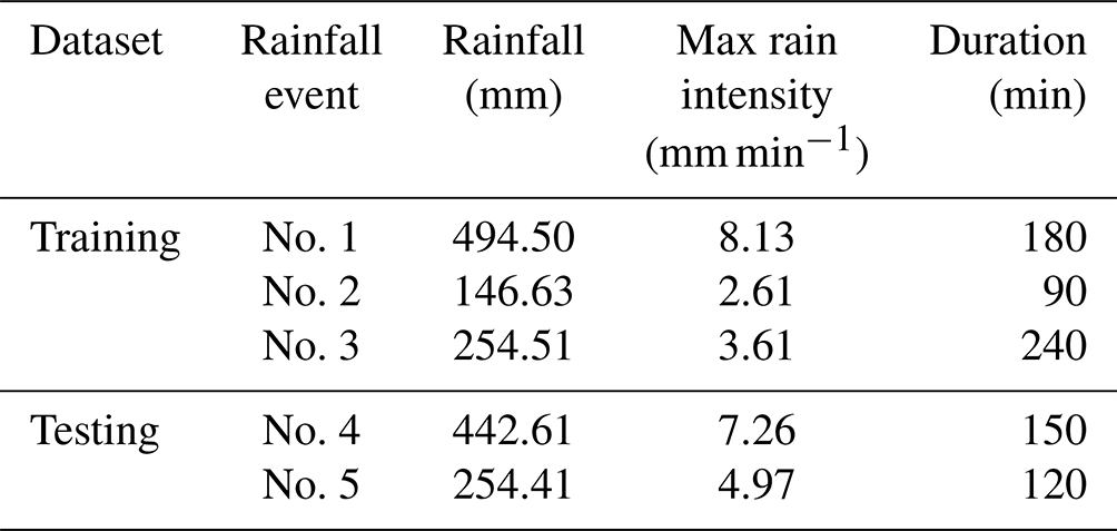
Besides, the measured rain data and monitoring data (water depth and flow) of five historical rainfall events were used to verify the performance of the corrected model. The uncertainty in the measurements was not considered (Huong and Pathirana, 2013). In this study, we considered the simulation results of the verified hydraulic model to be the ground truth.
Table 2 shows the measurements of the five historical rainfall events used in the process of model correction. Among the five events, three were used to correct model CR and the flow confluence process, while the other two were used to evaluate the reliability of the approach.
Table 2The five historical rainfall datasets used to correct the LSTM-based model.
2.4.4 Model construction
The hyperparameters used in this paper were mainly determined by Hyperopt (Bergstra et al., 2013). Hyperopt is a Python library for hyperparameter optimization that adjusts parameters using Bayesian optimization.
Table 3 shows the hyperparameters in the learning process of the model setup and model correction obtained by Hyperopt.
Table 3Hyperparameter configuration in the model setup and correction processes.

Note that the asterisks* refers to setting the hyperparameters of “CLASSIFICATION_MODULE” and “OUT_MODULE” in the flow confluence process to the same values. SGD is the stochastic gradient descent.
2.4.5 Performance evaluation
The mean absolute error (MAE), mean squared error (MSE), correlation coefficient (CC), and Nash–Sutcliffe efficiency coefficient (NSE) are broadly used indicators to assess the performance of a data-driven model. In this study, we used MAE and MSE to quantify the size of the errors; i.e., difference at each node between the prediction by the proposed LSTM-based model and simulation from the hydrodynamic model. Moreover, NSE and CC were also used to evaluate the level of agreement at all nodes. Equations (7)–(10) list the formulas of these four indicators.
where D is the number of events in the test set, T is the number of time steps of the relevant rainfall event, Yst is the prediction given by the neural network at the tth time step in the sth event, and is the simulation given by the hydrodynamic model.
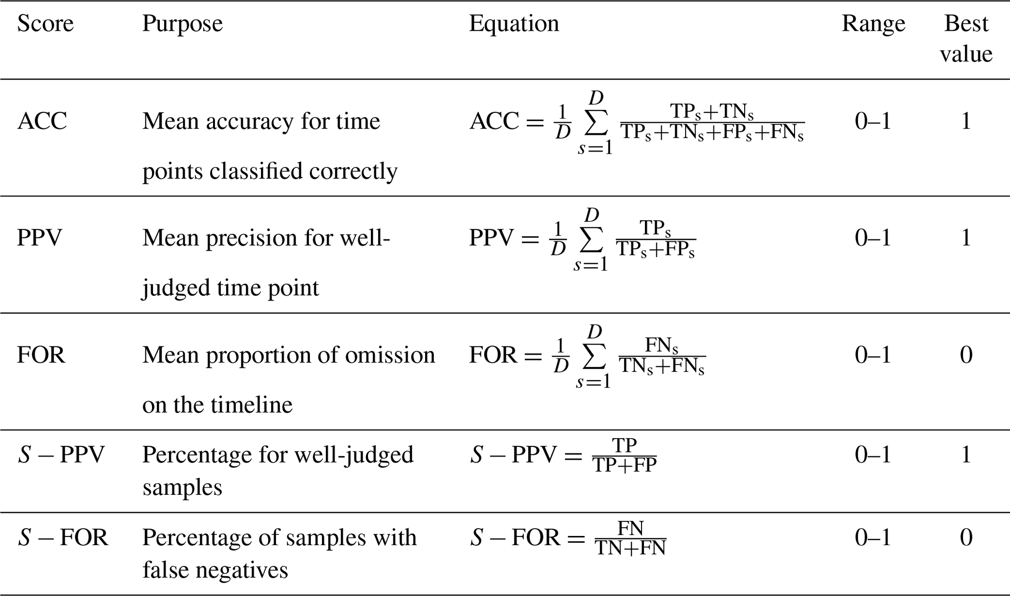
To evaluate the accuracy of the proposed model in predicting ponding, we have introduced five indicators (as shown in Table 4), namely accuracy (ACC), precision (PPV), and false omission rate (FOR) to evaluate the model accuracy in predicting the occurrence of ponding at a single node and S−PPV and S−FOR to evaluate the model accuracy in predicting the occurrence of ponding for a single event. TP and TN denote the number of occurrences when a ponding case and a normal case (no ponding occurs) are correctly identified, respectively, FP is the number of occurrences when a normal case is incorrectly identified as a ponding case, and FN is the number of occurrences when a ponding case is ignored by the model. The subscript “s” denotes the number of time steps in the sth event.
Table 4Indicators used to evaluate accuracy of the proposed model in predicting ponding for a single node and for a single event.
3.1 Model setup
The LSTM-based model was trained by the designed rainfall data and simulation produced from the hydrodynamic model. According to the procedures described in Sect. 2.2, the noise (ε) transmitted from the runoff process to the flow confluence process was equal to 1.9412 % in the case of the pipe network. For the sake of convenience, the noise was set to 2 %.
Figure 10 described the overall performance of the model using four box plots of the mean scores (of all nodes) on the test set, with the outliers removed. As shown in Fig. 10, the median values of MAE and MSE were much smaller than 0.1, indicating that the model has converged at all nodes. The median value of CC was close to 1, even though the minimum value was higher than 0.95. The median value of NSE was higher than 0.95, yet the minimum value was about 0.75, which indicated that, although the model's performance at each node was slightly different, the overall prediction was generally reliable.
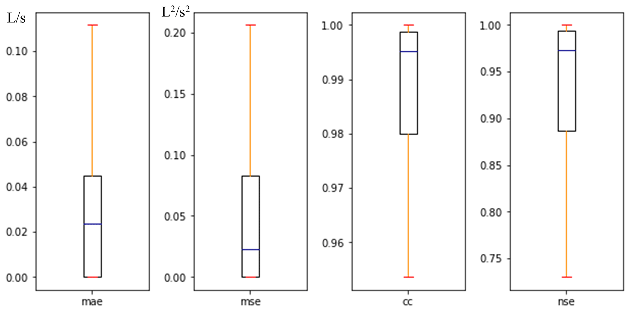
Figure 10Box plots of score values for comprehensive evaluation of all nodes in the case area in the model development procedure.
Due to the limited space, we only listed the evaluation results of six representative nodes. The six nodes (as shown in Fig. 11) were selected because of the severity of consequence once ponding occurred and also because they were relatively uniformly distributed in the pipe network. Moreover, three of them (nodes 2, 238, and 313) were chosen because the positive samples (where ponding occurred) accounted for less than 50 % of the training set, and the other three had the opposite case. For example, at node 238, the positive samples accounted for 18.33 % of the training set, while at node 95, up to 98.6 % samples were positive.

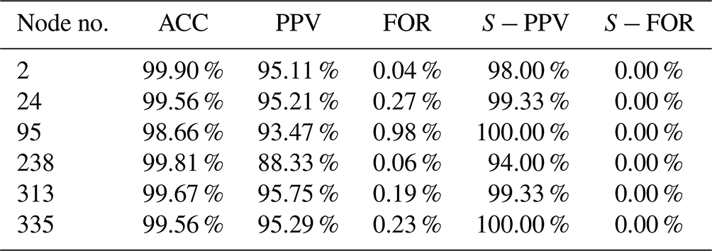
Table 5 lists the scores at the six selected nodes for evaluating the model performance in ponding occurrence prediction. In Table 5, columns ACC to FOR reflect the accuracy of ponding occurrence prediction in the sense of time (i.e., averaged in time). The mean ACC values (accuracy) for all six nodes were higher than 98.5 %. Compared to ACC, the mean PPV values (precision) were slightly lower, with the minimum value about 88 % at node 238, which indicated that a ponding case had at least an 88 % chance of being correctly identified. The mean FOR value (false omission rate) of each node was generally lower than 1 %, and among them the worst performance occurred at node 95 (FOR=0.98 %), which indicated that the model had a relatively small chance to ignore the ponding. The last two columns in Table 5 reflect the accuracy of the model in predicting ponding occurrence for a single rainfall event. For example, falsely reported events took up 6 % of the testing events at node 238 ( %), which was already the worst performance among the six selected nodes, while the S−FOR values at all of these six nodes equalled 0, which indicated that the model did not miss any ponding incidents in the testing set.
Table 5The scores at the six selected nodes for evaluating the model performance in ponding occurrence prediction.
The scores for evaluating the model performance in the ponding volume prediction are listed in Table 6. As shown in Table 6, the MAE and MSE scores were generally small, with the highest MAE score (0.0770 L s−1) occurring at node 95 and the highest MSE score (0.3788 L2 s−2) occurring at node 2. Compared to the MAE and MSE scores, the variability in the CC scores was much smaller. All of them were very close to 1. As for the NSE scores, the lowest score (NSE=0.8195 at node 238) was above 0.8. The results shown in Table 6 indicate that the proposed model had a relatively good performance in ponding volume prediction.
Table 6The scores at the six selected nodes for evaluating the model performance in ponding volume prediction.

Furthermore, in the above analysis, the mean score values on the test set were used for evaluation, and the variability was ignored. Figure 12 shows the predicted ponding volume at the selected nodes compared with the simulation results in six testing rainfall events. As shown in panel (1), the predicted start time of ponding was 5 min earlier than the simulation at node 2. As shown in panel (2), three peaks appeared in the ponding process of node 95, and the model has identified each of them. No ponding occurred at node 238, given the testing precipitation, as shown in panel (5), and the prediction of the model was in consistent with it. Overall, the prediction of the model was relatively accurate.
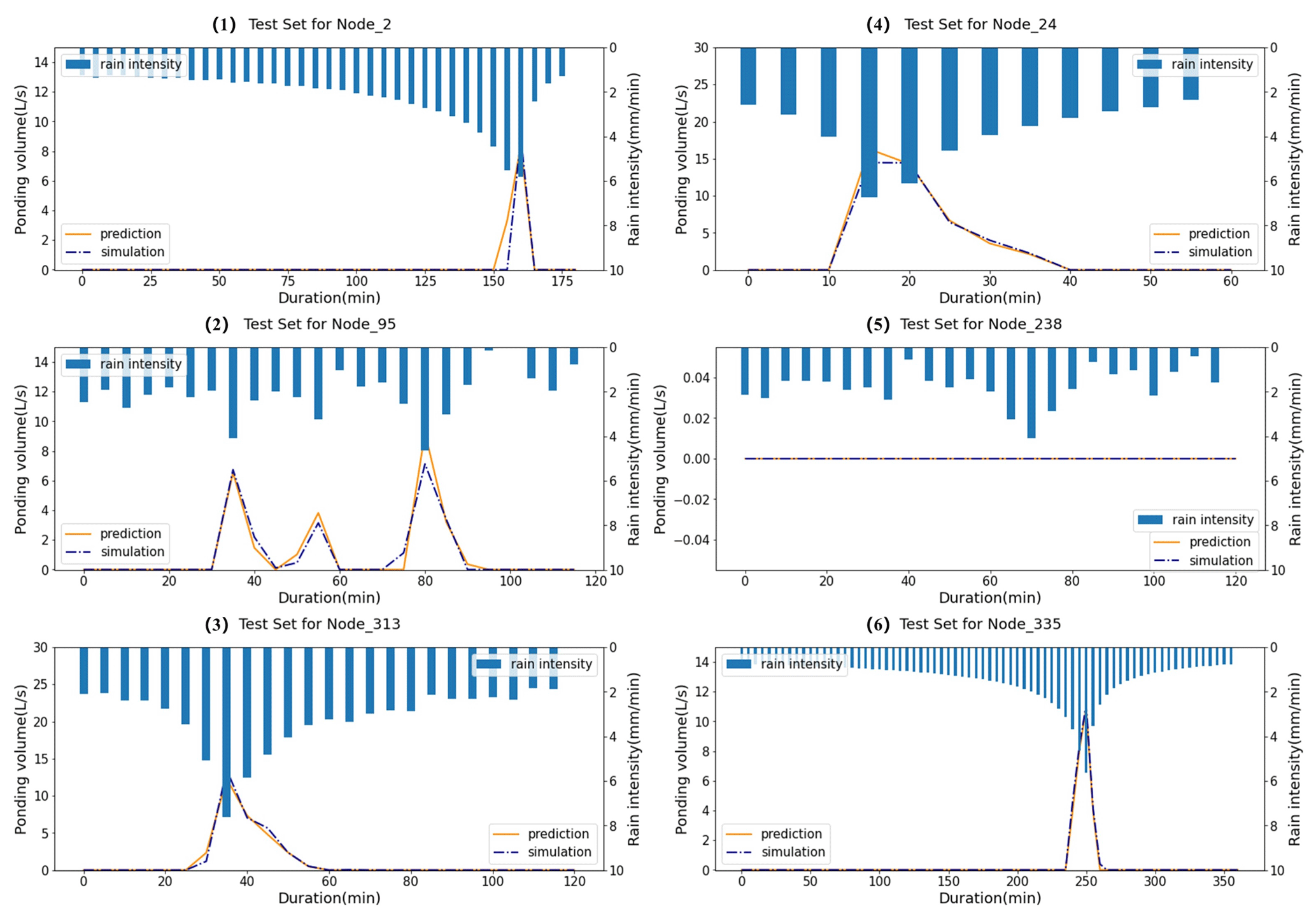
Figure 12Comparison between the predicted ponding volume and simulation from the hydrodynamic model at the selected nodes for six testing rainfall events that were chosen randomly.
3.2 Model correction
In this study, the model was trained based on the simulation results from a hydrodynamic model. Though the hydrodynamic model has been verified, the differences between the simulation (from the hydrodynamic model) at the monitoring points and the monitoring data persisted during the essential operation of the pipe network, which inevitably degraded the accuracy of the LSTM-based model in ponding forecast. Thus, it is necessary to correct the model using the measured rainfall data, level or flow data at the monitoring points, and ponding data.
The discrepancy between the measurements and simulation from the hydrodynamic model can be exemplified by Fig. 13. As shown in Fig. 13, rainfall event no. 5 was one of the measured precipitation events where the maximum precipitation intensity reached 4.97 mm min−1. For this event, the measured water depth and flow data were compared with the simulation from the hydrodynamic model, as shown in the left and right panels of Fig. 13, respectively.
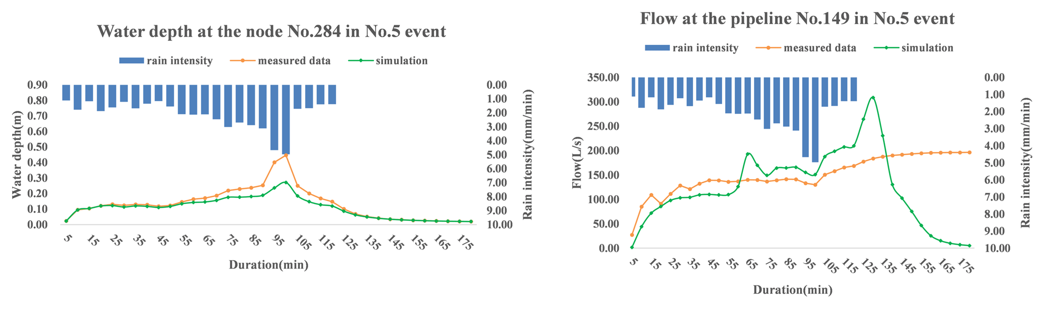
Figure 13Comparison between the measured data and simulation from the hydrodynamic model at node 284 and pipeline 149 for event no. 5.
The ponding process predicted by the corrected model was compared with the monitored ponding data to evaluate the model performance. Figure 14 illustrates the overall performance of the corrected model using four indicators, as described in Sect. 2.4.5. To be specific, the four box plots show the range of the mean score values on the test set at all nodes. As shown in the Fig. 14, the median values of the CC and NSE scores maintained values above 0.98 and 0.9, respectively. In contrast, the maximum values of MAE and MSE scores remained lower than 0.30 L s−1 and 0.6 L2 s−2, respectively.
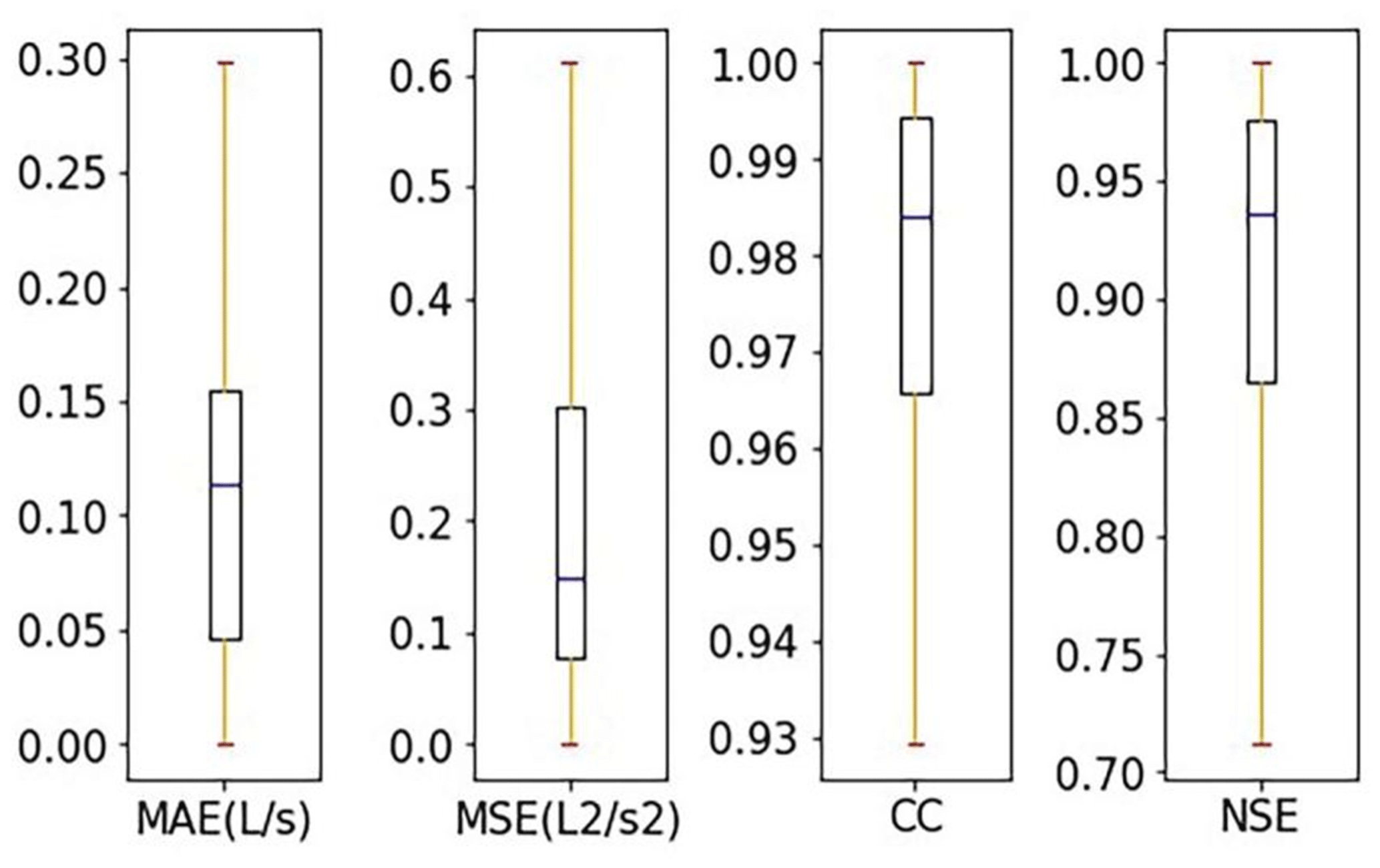
Figure 14Box plots of mean score values of the test set for all nodes in the model updating procedure.
Specifically, the mean score values at the six selected nodes obtained using the corrected model are summarized in Table 7. As shown in Table 7, the MAE and MSE scores were generally small, the NSE score at each node was stably above 0.9, and the CC scores were all above 0.95. The results shown in Table 7 suggest that the corrected model performed well at different nodes.
Table 7Mean score values at the six selected nodes obtained using the corrected model.
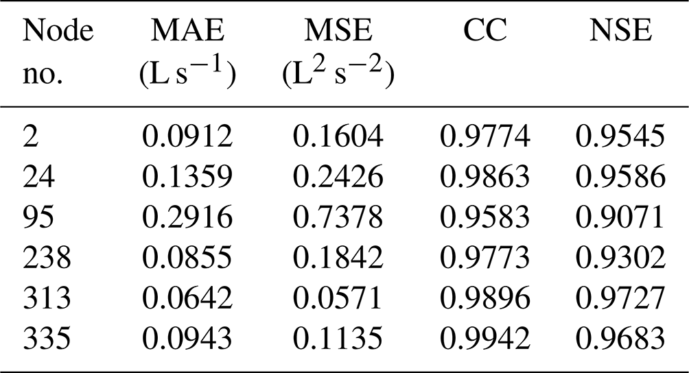
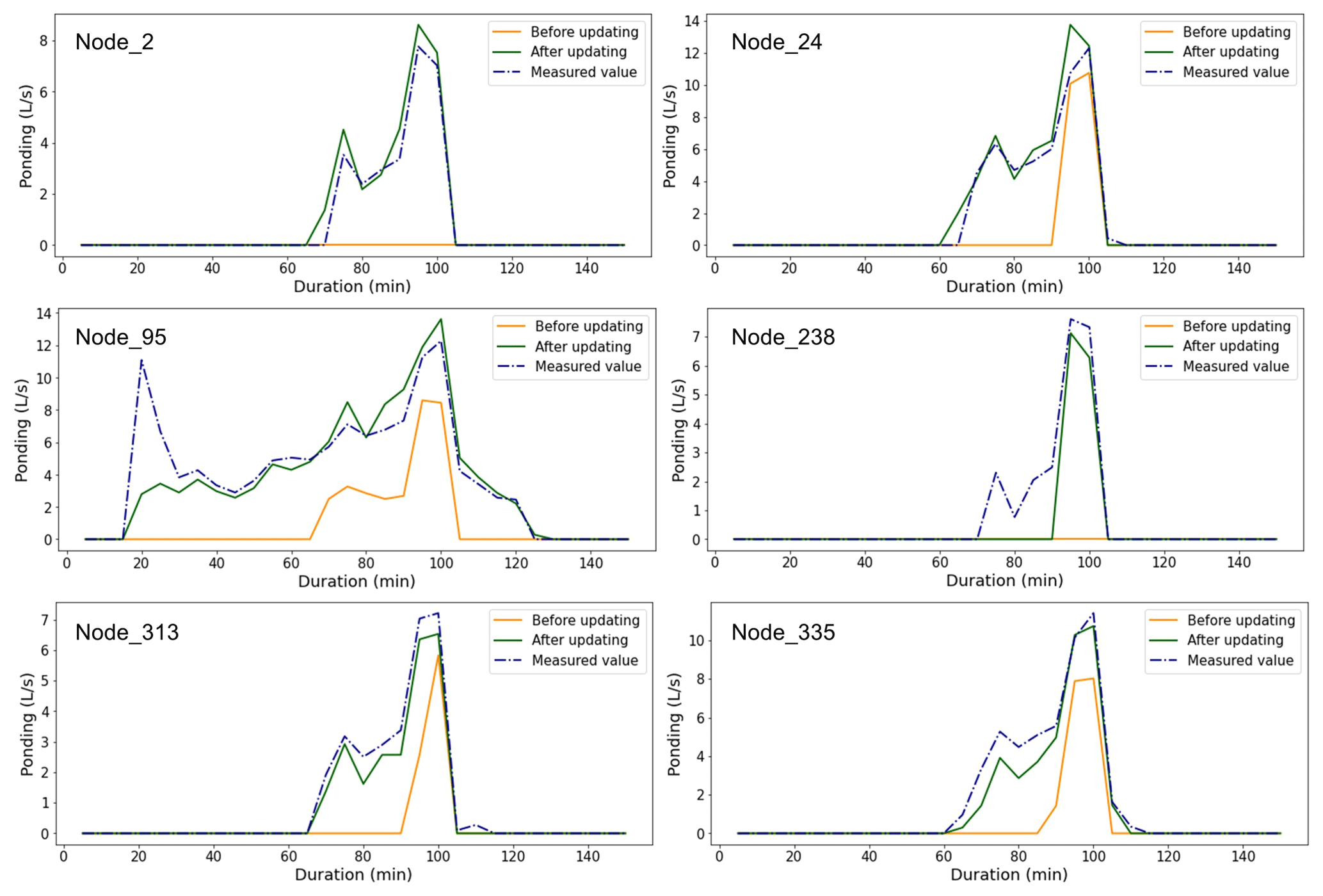
Figure 15Comparison between the predicted ponding volume and measured values at the selected nodes in rainfall event no. 5.
To further test the capability of the corrected model, the mean scores of all nodes for five measured rainfall events are summarized in Table 8, where the results from the model without correction are also listed as a comparison. As shown in Table 8, all of the four indicators suggest that the corrected model performed much better than the model without correction. Specifically, the NSE score obtained from the model without correction was less than 0, while this score rose up to 0.8316 after applying the model correction procedure, which indicated the necessity of the correction.
Table 8Mean score values of all nodes for five measured rainfall events, obtained by using the model with/without correction.

To further demonstrate the effect of model correction procedure, we have shown the predicted ponding process at the six selected nodes for rainfall event no. 5, obtained by using the model with and without correction, as shown in Fig. 15. As shown in Fig. 15, the corrected model performed better at all the selected nodes, e.g., by having a more accurate prediction of the start/end times of the ponding and more accurate ponding curves (more similar to the measured ones).
All of the results shown above demonstrate the superiority of the corrected model compared to the original one, in which the monitoring data were introduced in the model correction procedure.
4.1 Comparison of neural network structures
The proposed model (termed model A) was compared with the conventional LSTM structure (termed model B) to show the superiority of the variant of the LSTM structure in the flow confluence process. The schematic diagrams of the two models are shown in Fig. 16a–c. As shown in the various panels, model B has exactly the same structure as model A in the runoff process. The only difference in the two models lies in the flow confluence process, where a multi-task learning mechanism is introduced in the learning process of model A.

Figure 16Schematic diagrams of different network structures for comparison. (a) The same runoff process in models A and B. (b) The multi-target learning in the flow confluence process of model A (marked in light blue). (c) The flow confluence process in model B (marked in dark blue). (d) The LSTM structure in model C. (e) The CNN structure in model D.
Furthermore, model A, as proposed in this paper, was compared with two other models (models C and D) to illustrate the necessity of having the two processes in tandem, i.e., the runoff and flow confluence processes. The network structures of models C and D are shown in Fig. 16d and e, respectively, where the ponding information was obtained directly from the rainfall data without extracting the characteristics of lateral inflows.
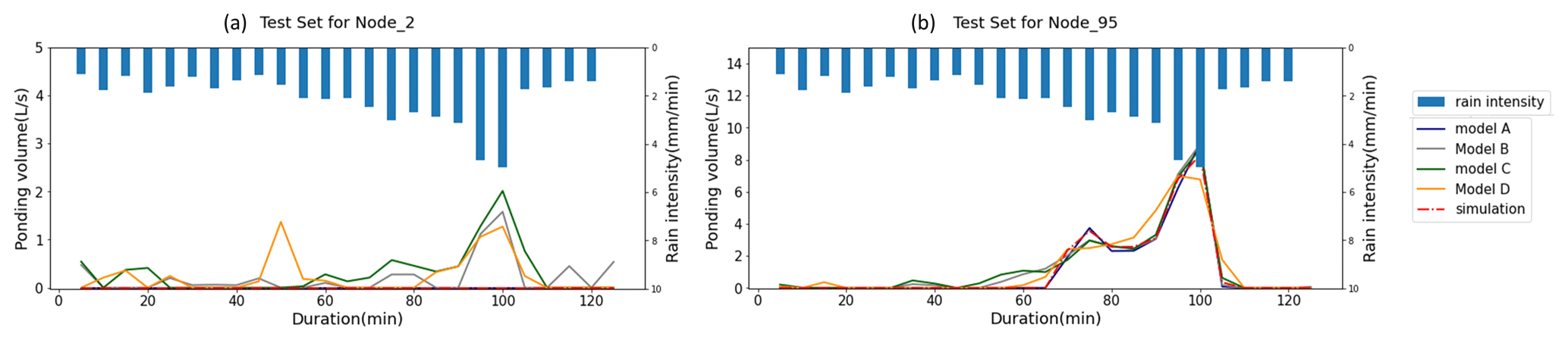
Figure 17A comparison between the predicted ponding volume by the LSTM-based model (model A) and by models B, C, and D for a particular rainfall event. (a) Case a, where ponding did not occur at node 2. (b) Case b, where ponding occurred at node 95.
Figure 17 shows two examples. In the first example, as shown in Fig. 17a, ponding did not occur at node 2. However, about 2–4 L s−1 ponding volume was falsely reported by the three alternative models (models B, C, and D), while model A predicted no ponding at this node, which was consistent with the simulation (considered to be the ground truth). In the second example, as shown in Fig. 17b, where ponding occurred and lasted for about 40 min, model A predicted a more accurate ponding curve than the other three alternative models.
Figure 18 presents the range of mean score values on the test set for all nodes, as obtained by using models A–D. As shown in the figure, the range of the MAE or MSE score from model A was half that of model B. The CC scores from model A were very close to 1, while the CC scores from model B varied from about 0.8 to 1. The NSE scores from model A were generally higher than 0.7, while the NSE scores from model B were unstable and generally lower than those from model A. Obviously, model A performed much better than model B in ponding volume prediction, as indicated by all four of the indicators.

Figure 18Comparison of model performance on the ponding volume forecasting. The results of the proposed model A are compared to those obtained from models B, C, and D.
As also shown in Fig. 18, the obvious superiority of model A (or B) over models C and D demonstrates the necessity of having two processes in tandem. Besides, it is also shown in Fig. 18 that the range of all four of these indicators expanded gradually from model A to D, which indicated decreased steadiness.
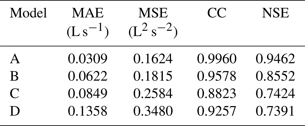
Table 9 shows the mean score values at all nodes (on the test set) obtained by using the four models. According to the results, the performance ranking of the four models was model A > model B > model C > model D.
Table 9Mean score values of all nodes obtained from models for predicting the volume of ponding.
The comparative analyses above indicated that the LSTM-based model proposed in this paper had remarkable superiority over the other three alternatives for ponding volume forecasting. There are two reasons behind this. First, the proposed model had two processes in tandem, namely the runoff and flow confluence processes. The second is due to the auxiliary classification task introduced in the flow confluence process. The two tandem processes reduced the computational burden of this data-driven approach and avoided interference with each other during training, while the classification task introduced facilitated the capability of the model to identify ponding.
4.2 The influence of the number of monitoring points on model correction
It was easy to spot from the trial that the performance of the corrected model depended on whether the layout of the monitoring points could reflect the hydraulic conditions of the pipe network. An unreasonable design of the monitoring equipment might lead to a failure in model correction.
There were 15 level gauges and 3 flowmeters in the case pipe network, as shown in Fig. 7b. To analyze how the number of monitoring points impacted the performance of the revised model, different numbers of monitoring points were randomly selected as a quantitative control group. Figure 19 presents the evaluation results of the revised model for ponding volume forecasting, as obtained by using different numbers of monitoring points.
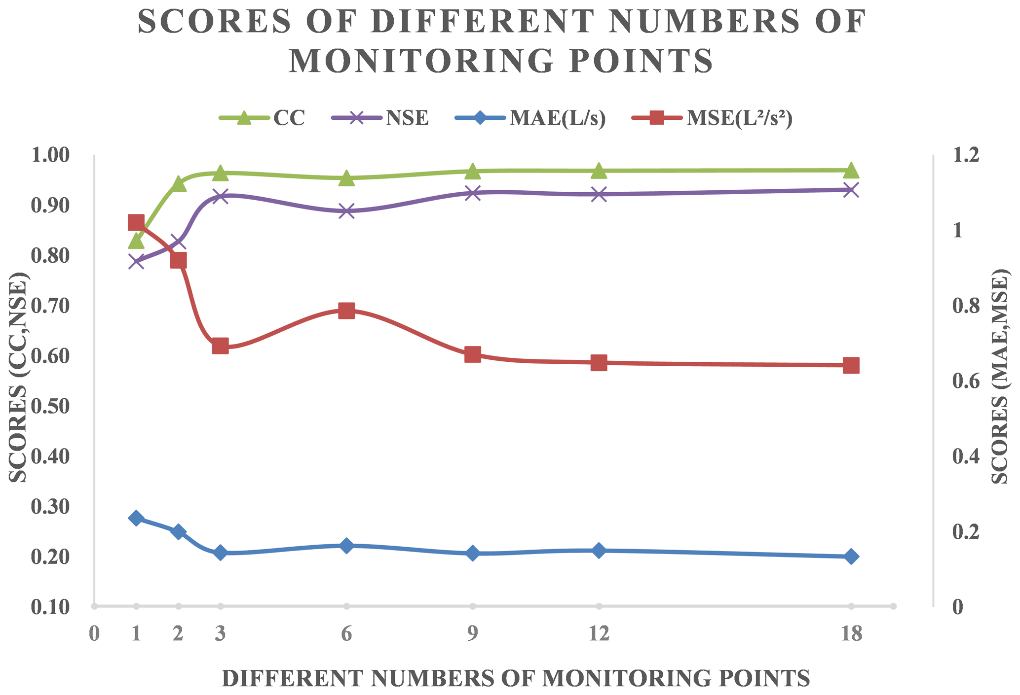
Figure 19Score values obtained by using different numbers of monitoring points in the model correction process.
As shown in the Fig. 19, the NSE scores stayed at around 0.9 when the number of monitoring points exceeded six, and the CC scores showed similar trends to the NSE scores. Besides, the other scores showed the opposite trends. It turned out that, when the number of monitoring points was over 1 per hectare, then increasing the number of monitoring points further had limited effect on improving the accuracy of the corrected model. However, when the number of monitoring points was below 0.5 per hectare (i.e., the number of monitoring points was less than 3), then it was highly effective to increase the number of monitoring points in the pipe network. For example, the NSE score was lower than 0.8 when the number of monitoring points was only 1.
In summary, one monitoring point per hectare is the critical point. If the number of monitoring points was less than this limit, then the performance of the revised model could not be guaranteed.
This work aims at promoting the application of deep learning in urban flood forecasting. Specifically, we have proposed an optimized LSTM-based approach in this study, which can quickly identify and locate ponding with relatively high accuracy.
According to the research results, the main conclusions of this study are summarized as follows:
-
The proposed model is constructed by two tandem processes (runoff process and flow confluence process) and utilizes a multi-task learning mechanism to achieve high accuracy. Over 15 000 designed rainfall events were used for model training, which covers various extreme weather conditions. The median score of NSE for ponding forecasting is greater than 0.95, and the mean accuracy at any node to determine whether ponding occurs reaches higher than 0.98.
-
The superiority of the proposed model has been demonstrated by comparing with two widely used deep learning models, namely (traditional) LSTM and CNN models.
The superiority of the proposed model having two tandem processes is proved by comparing with LSTM and CNN structures with a single process. The mean NSE score for the ponding volume forecasting of the proposed model is 0.9462, while those scores of the LSTM and CNN structures with a single process are 0.7424 and 0.7391, respectively. Then, the superiority of the proposed model with a LSTM variant is demonstrated by a comparison with the conventional LSTM structure that also has two tandem processes. As shown in Table 9, the mean NSE score of the latter is 0.8552.
-
An approach to the model modification using real-life monitoring level and flow data is proposed in this paper. The proposed LSTM-based model is further calibrated to achieve better accuracy.
The LSTM-based model is corrected using two steps. First, the runoff process is corrected with the measured rain, level, and flow data, referring to parameter-based (model-based) transfer learning. Then, the flow confluence process is updated using the updated lateral inflows at all nodes and the measured ponding volume. As shown in Table 8, the mean CC score at all nodes of the model with correction is 0.9309, while that of the model without correction is 0.1139.
Overall, the proposed LSTM-based approach provides a new possibility for early warning and forecasting of ponding in an urban drainage system. In this study, all operations were conducted in an offline mode. In a future study, we will explore the capability of the proposed model in a real-time event analysis. Furthermore, we will optimize the model by considering the influence of two-dimensional overland flow in ponding volume prediction.
The code used for all analyses and all data used in this study are available from the corresponding authors upon request.
WZ: methodology, formal analysis, visualization, software, and writing (original draft preparation). TT: conceptualization, funding acquisition, project administration, and writing (review and editing). HY: conceptualization, supervision, and validation. JY: writing (review and editing), supervision, and validation. JW: supervision and validation. SL: supervision and validation. KX: supervision and validation.
The contact author has declared that none of the authors has any competing interests.
Publisher's note: Copernicus Publications remains neutral with regard to jurisdictional claims in published maps and institutional affiliations.
The authors gratefully thank all the team members for their insightful comments and constructive suggestions that ensured a polished, high-quality paper.
This research has been supported by the National Natural Science Foundation of China (grant no. 51978493).
This paper was edited by Yue-Ping Xu and reviewed by two anonymous referees.
Abou Rjeily, Y., Abbas, O., Sadek, M., Shahrour, I., and Hage Chehade, F.: Flood forecasting within urban drainage systems using NARX neural network, Water Sci. Technol., 76, 2401–2412, https://doi.org/10.2166/wst.2017.409, 2017.
Archetti, R., Bolognesi, A., Casadio, A., and Maglionico, M.: Development of flood probability charts for urban drainage network in coastal areas through a simplified joint assessment approach, Hydrol. Earth Syst. Sci., 15, 3115–3122, https://doi.org/10.5194/hess-15-3115-2011, 2011.
Aryal, D., Wang, L., Adhikari, T. R., Zhou, J., Li, X., Shrestha, M., Wang, Y., and Chen, D.: A Model-Based Flood Hazard Mapping on the Southern Slope of Himalaya, Water, 12, 540, https://doi.org/10.3390/w12020540, 2020.
Bai, Y., Bezak, N., Sapač, K., Klun, M., and Zhang, J.: Short-Term Streamflow Forecasting Using the Feature-Enhanced Regression Model, Water Resour. Manage., 33, 4783–4797, https://doi.org/10.1007/s11269-019-02399-1, 2019.
Balstrøm, T. and Crawford, D.: Arc-Malstrøm: A 1D hydrologic screening method for stormwater assessments based on geometric networks, Comput. Geosci., 116, 64–73, https://doi.org/10.1016/j.cageo.2018.04.010, 2018.
Bergstra, J., Yamins, D., and Cox, D. D.: Making a science of model search: hyperparameter optimization in hundreds of dimensions for vision architectures, in: Proceedings of the 30th International Conference on International Conference on Machine Learning – Volume 28, JMLR.org, Atlanta, GA, USA, I-115–I-123, https://doi.org/10.5555/3042817.3042832, 2013.
Cai, B. and Yu, Y.: Flood forecasting in urban reservoir using hybrid recurrent neural network, Urban Climate, 42, 101086, https://doi.org/10.1016/j.uclim.2022.101086, 2022.
Chiang, Y.-M., Chang, L.-C., Tsai, M.-J., Wang, Y.-F., and Chang, F.-J.: Dynamic neural networks for real-time water level predictions of sewerage systems-covering gauged and ungauged sites, Hydrol. Earth Syst. Sci., 14, 1309–1319, https://doi.org/10.5194/hess-14-1309-2010, 2010.
Djordjević, S., Prodanović, D., and Maksimović, Č.: An approach to simulation of dual drainage, Water Sci. Technol., 39, 95–103, https://doi.org/10.1016/S0273-1223(99)00221-8, 1999.
Djordjević, S., Prodanović, D., Maksimović, Č., Ivetić, M., and Savić, D.: SIPSON – Simulation of Interaction between Pipe flow and Surface Overland flow in Networks, Water Sci. Technol., 52, 275–283, https://doi.org/10.2166/wst.2005.0143, 2005.
Guo, K., Guan, M., and Yu, D.: Urban surface water flood modelling – a comprehensive review of current models and future challenges, Hydrol. Earth Syst. Sci., 25, 2843–2860, https://doi.org/10.5194/hess-25-2843-2021, 2021.
Hossain Anni, A., Cohen, S., and Praskievicz, S.: Sensitivity of urban flood simulations to stormwater infrastructure and soil infiltration, J. Hydrol., 588, 125028, https://doi.org/10.1016/j.jhydrol.2020.125028, 2020.
Huong, H. T. L. and Pathirana, A.: Urbanization and climate change impacts on future urban flooding in Can Tho city, Vietnam, Hydrol. Earth Syst. Sci., 17, 379–394, https://doi.org/10.5194/hess-17-379-2013, 2013.
Jamali, B., Löwe, R., Bach, P. M., Urich, C., Arnbjerg-Nielsen, K., and Deletic, A.: A rapid urban flood inundation and damage assessment model, J. Hydrol., 564, 1085–1098, https://doi.org/10.1016/j.jhydrol.2018.07.064, 2018.
Kao, I., Zhou, Y., Chang, L., and Chang, F.: Exploring a Long Short-Term Memory based Encoder-Decoder framework for multi-step-ahead flood forecasting, J. Hydrol., 583, 124631, https://doi.org/10.1016/j.jhydrol.2020.124631, 2020.
Keifer, C. J. and Chu, H. H.: Synthetic Storm Pattern for Drainage Design, J. Hydraul. Div., 83, 1332-1–1332-25, https://doi.org/10.1061/JYCEAJ.0000104, 1957.
Kratzert, F., Klotz, D., Herrnegger, M., Sampson, A. K., Hochreiter, S., and Nearing, G. S..: Toward Improved Predictions in Ungauged Basins: Exploiting the Power of Machine Learning, Water Resour. Res., 55, 11344–11354, https://doi.org/10.1029/2019WR026065, 2019a.
Kratzert, F., Klotz, D., Shalev, G., Klambauer, G., Hochreiter, S., and Nearing, G.: Towards learning universal, regional, and local hydrological behaviors via machine learning applied to large-sample datasets, Hydrol. Earth Syst. Sci., 23, 5089–5110, https://doi.org/10.5194/hess-23-5089-2019, 2019b.
Kuczera, G., Lambert, M., Heneker, T., Jennings, S., Frost, A., and Coombes, P.: Joint probability and design storms at the crossroads, Aust. J. Water Resour., 10, 63–79, https://doi.org/10.1080/13241583.2006.11465282, 2006.
Leandro, J. and Martins, R.: A methodology for linking 2D overland flow models with the sewer network model SWMM 5.1 based on dynamic link libraries, Water Sci. Technol., 73, 3017–3026, https://doi.org/10.2166/wst.2016.171, 2016.
Löwe, R., Böhm, J., Jensen, D. G., Leandro, J., and Rasmussen, S. H.: U-FLOOD – Topographic deep learning for predicting urban pluvial flood water depth, J. Hydrol., 603, 126898, https://doi.org/10.1016/j.jhydrol.2021.126898, 2021.
Moy De Vitry, M., Kramer, S., Wegner, J. D., and Leitao, J. P.: Scalable flood level trend monitoring with surveillance cameras using a deep convolutional neural network, Hydrol. Earth Syst. Sci., 23, 4621–4634, https://doi.org/10.5194/hess-23-4621-2019, 2019.
Mudashiru, R. B., Sabtu, N., Abustan, I., and Balogun, W.: Flood hazard mapping methods: A review, J. Hydrol., 603, 126846, https://doi.org/10.1016/j.jhydrol.2021.126846, 2021.
Pan, S. J. and Yang, Q.: A Survey on Transfer Learning, IEEE T. Knowl. Data Eng., 22, 1345–1359, https://doi.org/10.1109/TKDE.2009.191, 2010.
Pilgrim, D. H. and Cordery, I.: Rainfall Temporal Patterns for Design Floods, J. Hydraul. Div., 101, 81–95, https://doi.org/10.1061/JYCEAJ.0004197, 1975.
Rahman, A., Weinmann, P. E., Hoang, T. M. T., and Laurenson, E. M.: Monte Carlo simulation of flood frequency curves from rainfall, J. Hydrol., 256, 196–210, https://doi.org/10.1016/S0022-1694(01)00533-9, 2002.
Shen, C.: A Transdisciplinary Review of Deep Learning Research and Its Relevance for Water Resources Scientists, Water Resour. Res., 54, 8558–8593, https://doi.org/10.1029/2018WR022643, 2018.
Sit, M., Demiray, B. Z., Xiang, Z., Ewing, G. J., Sermet, Y., and Demir, I.: A Comprehensive Review of Deep Learning Applications in Hydrology and Water Resources, ResearchGate, https://doi.org/10.31223/osf.io/xs36g, 2020.
Skougaard Kaspersen, P., Høegh Ravn, N., Arnbjerg-Nielsen, K., Madsen, H., and Drews, M.: Comparison of the impacts of urban development and climate change on exposing European cities to pluvial flooding, Hydrol. Earth Syst. Sci., 21, 4131–4147, https://doi.org/10.5194/hess-21-4131-2017, 2017.
Teng, J., Jakeman, A. J., Vaze, J., Croke, B. F. W., Dutta, D., and Kim, S.: Flood inundation modelling: A review of methods, recent advances and uncertainty analysis, Environ. Model. Softw., 90, 201–216, https://doi.org/10.1016/j.envsoft.2017.01.006, 2017.
Tian, F., Ma, B., Yuan, X., Wang, X., and Yue, Z.: Hazard Assessments of Riverbank Flooding and Backward Flows in Dike-Through Drainage Ditches during Moderate Frequent Flooding Events in the Ningxia Reach of the Upper Yellow River (NRYR), Water, 11, 1477, https://doi.org/10.3390/w11071477, 2019.
Xiang, Z., Yan, J., and Demir, I.: A Rainfall-Runoff Model With LSTM-Based Sequence-to-Sequence Learning, Water Resour. Res., 56, e2019WR025326, https://doi.org/10.1029/2019WR025326, 2020.
Zhang, S. and Pan, B.: An urban storm-inundation simulation method based on GIS, J. Hydrol., 517, 260–268, https://doi.org/10.1016/j.jhydrol.2014.05.044, 2014.