the Creative Commons Attribution 4.0 License.
the Creative Commons Attribution 4.0 License.
 | 26 May 2023
A mixed distribution approach for low-flow frequency analysis – Part 2: Comparative assessment of a mixed probability vs. copula-based dependence framework
In climates with a warm and a cold season, low flows are generated by different processes, which violates the homogeneity assumption of extreme value statistics. In this second part of a two-part series, we extend the mixed probability estimator of the companion paper (Laaha, 2023) to deal with dependency of seasonal events. We formulate a copula-based estimator for seasonal minima series and examine it in a hydrological context. The estimator is a valid generalization of the annual probability estimator and provides a consistent framework for estimating return periods of summer, winter, and annual events. Using archetypal examples we show that differences in the mixed estimator are always observed in the upper part of the distribution, which is less relevant for low-flow frequency analysis. The differences decrease as the return period increases so that both models coincide for the severest events. In a quantitative evaluation, we test the performance of the copula estimator on a pan-European data set. We find a large gain of both mixed distribution approaches over the annual estimator, making these approaches highly relevant for Europe as a whole. We then examine the relative performance gain of the mixed copula versus the mixed distribution approach in more detail. The analysis shows that the differences in the 100-year event are actually minimal. However, the differences in 2-year events are considerable in some of the catchments, with a relative deviation of −15 % to −25 % in the most affected regions. This points to a prediction bias of the mixed probability estimator that can be corrected using the copula approach. Using multiple regression models, we show that the performance gain can be well explained on hydrological grounds, with weak seasonality leading to a high potential for corrections and strong seasonal correlation reinforcing the need to take this potential into account. Accordingly, the greatest differences can be observed in mid-mountain regions in cold and temperate climates, where rivers have a strongly mixed low-flow regime. This finding is of particular relevance for event mapping, where regional severity can be misinterpreted when the seasonal correlation is neglected. We conclude that the two mixed probability estimators are quite similar, and both are conceptually more adequate than the annual minima approach for mixed summer and winter low-flow regimes. In regions with strong seasonal correlation the mixed copula estimator appears most appropriate and should be preferred over the mixed distribution approach.
- Article
(6449 KB) - Full-text XML
- Companion paper
- BibTeX
- EndNote


In seasonal climates with a warm and a cold season, low flows are generated by different processes so that the annual extreme series will be a mixture of summer and winter low-flow events. This can violate the basic assumption of extreme value statistics and give rise to inaccurate conclusions. In the first part of the study (Laaha, 2023) we addressed the problem of process heterogeneity by proposing a mixed probability estimator for annual minimum flows (low-flow magnitude) that combines the seasonal distributions. Compared to the conventional estimator, we showed that the estimator can indeed estimate return periods more accurately.
In this second part of the study, we address the problem when summer and winter minima are not completely independent. This can play a role in low-flow statistics, where the events have a long timescale and may last for several months or even some years (Stahl and Hisdal, 2004). Although not all events span such a long time period, there are instances where summer low flows are continued by a winter low-flow event. Van Loon et al. (2015) found this drought type quite common in cold temperate climates, whereas the reverse case of a prolonged winter drought appeared to be less frequent. Prolonged low-flow events need not be extreme in both seasons, but some dependence between seasonal minima must still be expected. For such cases, the mixed probability model can be extended by using a multivariate distribution approach.
The use of multivariate distributions for extremes dates back to Gumbel (1960) and has a long tradition in hydrology. A well-known problem in flood frequency analysis is that the extreme event cannot be fully described by the peak of the event alone, but additional aspects such as duration and volume must be considered. Yue et al. (1999) employed a bivariate Gumbel distribution model to perform a consistent frequency analysis of correlated pairs of variables, such as peak and volume, as well as volume and duration. The model was found to be well suited to represent the joint occurrence probability of flood characteristics. The approach uses an analytical formulation of the multivariate distribution model, which, however, exists only for some distribution families. In the cases where no analytical expression exists, the joint probability model can be constructed using a copula approach.
Copula models have recently received increasing attention in hydrology. Most examples are for flood frequency analysis but some examples for droughts and low flows also exist. A good overview of copula theory with respect to hydrological applications is given in Klein et al. (2011). Renard and Lang (2007) demonstrated the value of Gaussian copula models for a variety of problems where two or more variables are required for inference. Examples include field significance in multiple testing problems (e.g. regional trend analysis), regional risk assessment that combines at-site risks at the regional scale, joint assessment of discharge–duration–frequency of design events, and incorporation of intersite dependence in regional flood frequency analysis. The paper showed the usefulness of the multivariate approach but underlined the limitation of being restricted to a Gaussian copula model. Poulin et al. (2007) found that extreme event characteristics have a particular tail dependence for which the Gumbel and survival Clayton copula models should be most adequate. This was also confirmed in the case study of Ganguli and Reddy (2012), where based on the tail-dependence measure the Gumbel–Hougaard copula was found to be the best-suited model for capturing the joint dependence between meteorological drought severity and duration. Fischer and Schumann (2021) again used vine copulas to determine the most probable combinations of flood types for tributaries. Klein et al. (2011) further demonstrated the potential of copulas for dam safety analysis. They used a bivariate copula distribution model to define joint return periods of critical flood peak and volume events, which allowed them to better assess the effect of flood protection measures for dam safety based on their marginal effects. Finally, another application of copulas can be found in Ganguli and Reddy (2014), where a copula-based model between predicted and observed drought index values was used to simulate predictive uncertainty of meteorological drought forecasts.
In a low-flow hydrologic context, bivariate analysis of volume and duration of below-threshold events was performed by Ashkar et al. (1998) using a bivariate exponential distribution. They found the applicability of the method depending on the strength of the correlation of the two variables. Sahoo et al. (2020) used a bivariate copula distribution model to analyse cumulative annual drought duration and volume below the Q75 threshold (i.e. the flow percentile with exceedance probability of 75 %) for two stations in an Indian study area. They found the general extreme value distribution (GEV) in combination with a Clayton and Frank copula model were best suited in both stations; however the differences between the copula models appeared to be small and depended on the criterion used for model selection. This view is supported by Genest and Favre (2007), who found the difference between different extreme value copula models to be mostly negligible, and choosing between them would not make any serious difference for prediction purposes. Ahn and Palmer (2016) used a non-stationary copula to predict future bivariate low-flow frequency in the Connecticut River basin. In the absence of stationarity, the model was shown to provide more accurate frequency estimates than the stationary model alternatives. A similar approach was used by Jiang et al. (2015) to perform a bivariate frequency analysis for the low-flow series from two neighbouring hydrological gauges. The study extended the scope of the regional model by Ahmadi et al. (2018), who used a stationary copula model to define the dependency structure of the low-flow magnitude of tributaries.
While copula approaches have been used to combine either different event characteristics (e.g. volume and duration) in a local analysis or the same event characteristic at multiple sites, we are not aware of any study that has used copulas to account for seasonal dependence in a mixed distribution approach to modelling the frequency of extreme events. In this second paper, we propose such a mixed copula estimator based on annual and seasonal minima series to conduct low-flow frequency analysis for mixed seasonal regimes. The aims of the paper are as follows:
-
to formulate an enhanced mixed distribution approach for minima that incorporates seasonal correlation,
-
to review its behaviour and plausibility for archetypal catchments,
-
to evaluate its possible performance gain compared to the mixed probability estimator,
-
to give a recommendation of which estimator to use under specific hydrological conditions.
The paper will also extend the analysis of the companion paper (Laaha, 2023) to the pan-European level to assess the value of mixed distribution approaches for a greater variety of hydrologic regimes.
2.1 Theoretical probability estimator
Let us consider the case where the annual minima series is composed of events that arise from different processes occurring in the summer and winter season. Here, the annual minima series AM can be viewed as the minima of the annual summer minima AMS and winter minima AMW:
These constitute samples from two random variables, annual summer low flow S and annual winter low flow W. Assuming independence of summer and winter events, the probability of a low-flow event with magnitude q can be obtained from its occurrence probabilities in the summer season and winter season using the multiplication rule of statistics. By the notation F⋅(q) we make explicit that the same flow (i.e. the event magnitude of interest) is inserted into both marginal distributions. In this case, the mixed probability estimator can be written analogous to Stedinger et al. (1993) as
It offers a valid generalization of the annual frequency estimator that yields improved probability estimates in the case of differing summer and winter distributions (Laaha, 2023).
The multiplication rule is just a special case of a more general problem of frequency analysis where we are concerned with finding the joint occurrence probability of events in two variables. This can be solved by bivariate frequency analysis. Here, a bivariate probability model is used to estimate the joint probability that S and W are less than or equal to the magnitudes s and w, respectively:
In this paper we propose a copula-based approach to model the bivariate frequency distribution . A copula C(⋅) is a function which exactly describes and models the dependency structure between correlated random variables independently of their marginal distributions (Klein et al., 2011). The link between the copula and the multivariate distribution is provided by the theorem of Sklar (1959) so that the joint cdf can be written as
The approach requires the choice of a copula model. As we are modelling extreme values, a Gumbel–Hougaard copula may be an adequate choice. The model can be written as
where u and v denote the so-called pseudo-observations corresponding to the empirical probabilities of S and W, respectively. The parameter θ is used to model the strength of the dependency structure of the distributions. It is directly linked to the correlation (Kendall's τ), with θ=1 denoting the case of complete independence. However, since the adequate model is a priory unknown, alternative copula families can be considered as well. In this case the best-suited model can be chosen based on a copula information criterion (Grønneberg and Hjort, 2014).
The model can now be used to estimate the occurrence probability of a low-flow event by inserting its magnitude q into both marginal distributions. This yields to its summer and winter occurrence probabilities FS(q) and FW(q), respectively. The (joint) probability that S and W both fall below q is given by the so-called AND operator (Klein et al., 2011, Eq. 8.29 for maxima). Applying the AND operator to minima yields the copula-based mixed probability estimator of annual low-flow occurrences:
All considered models are reduced to the independence copula for the case of independent events, where C[FS(q),FW(q)] becomes FS(q)⋅FW(q) and Eq. (6) simplifies to Eq. (2) accordingly. The mixed copula estimator is therefore a valid generalization of the mixed distribution estimator proposed in the companion paper (Laaha, 2023) for the case where summer and winter low flows are not completely independent. As in the companion paper, we employ a Weibull distribution, with marginal summer distribution
and marginal winter distribution
to model the distributions of seasonally separable events. ζ⋅, β⋅, and δ⋅ are the location, scale, and shape parameters of summer (index S) and winter (index W) distributions, respectively.
2.2 Empirical probability estimator
In the same way as for the theoretical estimator, we can also define an empirical estimator that generalizes the mixed probability approach to the case of seasonal correlation.
Table 1Overview of the example gauges used for model demonstration. Shown are the station identifier (ID), catchment area (AREA), Spearman's correlation between summer and winter event series (ρ) together with its significance level (p value), the mean resultant of the circular seasonality index (r), and the seasonality ratio (SR) representing the ratio between mean summer and mean winter low flow.

Let q be an element of an annual minima series AM with n observations and m its rank in increasing order. Assuming that the AM is sampled from (a sequence of) independent and identically distributed random variables, thus iid, the empirical probability p of a low-flow event with magnitude q can be calculated by
The iid assumption implies that the annual minima are generated by the same low-flow process (i.e. are homogeneous) and are not correlated. In the case where the sample is heterogeneous and possibly correlated, a generalized estimator can be obtained from bivariate frequency analysis. Assuming seasonally separable low-flow distributions, the generalized empirical probability can be formulated in accordance with the theoretical probability estimator in Eq. (6) as
where pS(q) and pW(q) denote the probability of q occurring in the summer season and the winter season, respectively. Cn(⋅) is the empirical copula, which defines the empirical multivariate distribution analogous to Eq. (4). In contrast to the theoretical copula, no parametric model has to be assumed to calculate the empirical probability. The estimator can be rewritten as
using mS and nS for the rank and sample size of the summer minima series and mW and nW of the winter minima series, respectively.
Like any empirical probability estimator, pmix,C is susceptible to sampling uncertainties and therefore mainly used in distribution plots to visualize the fit of the theoretical distribution to observations. In contrast to the common empirical estimator, the magnitude q of the annual series may be missing from the marginal series, and its empirical probability must be approximated. Such an approximation is obtained by averaging the rank of the next smaller and bigger elements to q in the marginal series, in accordance with Laaha (2023).
2.3 Demonstration of model behaviour
As in the companion paper we use archetypal examples to demonstrate the behaviour of the model. The examples used now differ not only in terms of the strength of seasonality, but also in terms of seasonal correlation, ranging from insignificant correlations to highly correlated summer and winter events. An overview is given in Table 1. Seasonality is characterized by the seasonality ratio (SR), where SR>1 indicates a winter and SR<1 a summer low-flow regime, and the mean resultant of the circular seasonality index (r), where a value of 0 represents the weakest and a value of 1 the strongest possible seasonality. Further details about the indices are given in Sect. 3.3.
The first example is the Ebensee gauge at river Langbathbach, representing the case of almost no seasonality (SR=1.09) and insignificant seasonal correlation, as indicated by a Spearman's ρ of 0.22 and a p value of 0.20. The gauge was also used in the companion paper, as it represents a typical foreland catchment, where discharges from the mountains and lowlands mix. The mixed distribution approach has been shown to differ strongly from the annual distribution fitted to the heterogeneous series in this case. Since the assumption of independence of seasonal low flows cannot be rejected, it is reasonable to assume that there is not much difference between the mixed distribution approach and the copula-based estimator. Figure 1a shows that there is indeed almost no difference between the two estimators in the lower part of the distribution, which is relevant for low-flow frequency analysis. There are differences in the upper part of the distribution, however, where the mixed distribution falls much below the annual estimator. The mixed copula approach corrects a large part of this deviation. It brings the mixed distribution close to the annual one, which has previously been shown to be appropriate in the central part of the distribution where the summer and winter distributions coincide.
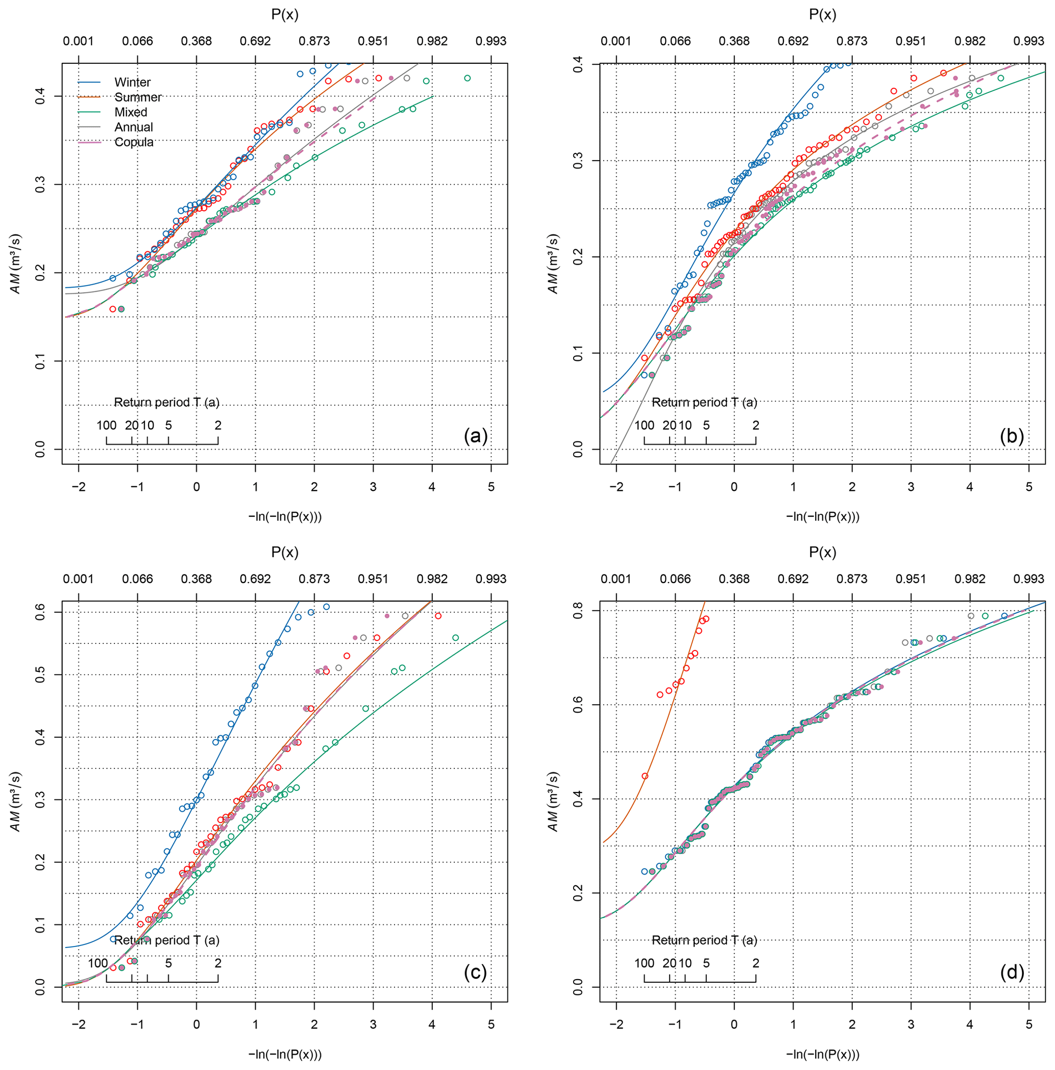
Figure 1Probability plots of summer (red), winter (blue), annual (grey), mixed (green), and mixed copula (magenta) distributions for archetypal cases: (a) Ebensee at river Langbathbach situated in the northern foothills of the Alps of Upper Austria; (b) Weg at river Isen situated in low, hilly terrain in Bavaria, Germany; (c) Trausdorf an der Wulka at river Wulka situated in the eastern foreland of the Alps in Burgenland, Austria; and (d) Schalklhof at river Schalklbach representing an alpine catchment in Tyrol, Austria. The copula estimator is calculated using the Gumbel–Hougaard family.
The second example is gauge Weg at river Isen situated in low, hilly terrain in Bavaria, Germany, representing the case of weak summer seasonality (SR=0.87) combined with moderate seasonal correlation (ρ=0.44). The gauge was also used in the companion paper to show that substantial mixing can occur even in cases where one seasonal distribution is always lower than the other but in this case not in the most extreme low-flow events. It was shown that the mixed probability estimator reflects this behaviour by following the dominant distribution at the lower tail and combining the probabilities in the range of discharges where low flows in both seasons occur. Figure 1b shows that despite the now-significant correlation (p value < 0.01), both mixed probability approaches coincide at the lower part of the distribution. As in the Ebensee gauge example, there is some deviation between the mixed and the annual distribution at higher low flows, which is again reduced by the mixed copula estimator. We note that this behaviour is only observed at the upper part of the distribution, which is less relevant for low-flow statistics. At most, there is a slight difference in moderate low-flow events with a return period of T=2 years, but this should have little effect on the estimated return periods for the given case.
The third example is gauge Trausdorf an der Wulka at river Wulka situated in the eastern foreland of the Alps in Burgenland, Austria. It represents the case of a medium-sized lowland catchment (AREA=236 km2) with significant tributaries from the Alps. Low flows in the catchment have a strong seasonal correlation (ρ=0.71) and moderate summer seasonality (SR=0.74). Because of the strong correlation we can expect there is a large difference between the mixed distribution approach and the copula-based estimator. This is indeed visible from Fig. 1c. There is still a part where both mixed distribution approaches coincide, but this is much smaller and is restricted to return periods of T=10 years and more. For lower return periods, the mixed distribution falls far below the dominant summer distribution, and this difference is to a large extent corrected by the mixed copula estimator.
The fourth and final example is gauge Schalklhof at river Schalklbach representing a medium-sized alpine catchment (AREA=108 km2) in Tyrol, Austria. The catchment represents the ultimate case of a significant seasonal correlation (ρ=0.27 with a p value < 0.05) combined with a very strong winter seasonality (SR=2.52). In this case there is almost no mixture of summer and winter discharges, making it irrelevant whether they are correlated or not. Figure 1d shows that all distributions apart from the subordinate summer distribution coincide, so there is no gain of the mixed copula estimator over the mixed probability estimator. Moreover, there is also no gain of the mixed distribution approaches over the annual estimator at all, as the annual distribution and the winter distribution coincide. In the companion paper it was noted that such cases are rare in the Austrian study area and limited to high-alpine catchments. We expect them to play a subordinate role in the European data set as well.
On the whole, the examples suggest that there is little difference between the two mixed estimators in the lower part of the distribution, so using the copula-based approach should have little effect on the estimated return period of an event. Seasonal correlation is observed to affect mainly the upper part of the distribution, which is less relevant for low-flow analysis. Although the differences between the two mixed probability estimators tend to be small, they increase with increasing correlation and may become relevant for highly correlated cases. In the following, we assess the possible gains of the mixed copula estimator based on a comprehensive pan-European data set.
3.1 Pan-European assessment
The model is evaluated based on a pan-European data set. We use the data selection of Laaha et al. (2017) and Stahl et al. (2020) consisting of about 800 gauges across Europe with daily measurements for the period 1976–2010. Most data are available from the Global Runoff Data Centre (GRDC) portal https://portal.grdc.bafg.de (last access: 8 November 2022). The selected stations are free from major disturbances of the low-flow regime. These include 673 series with complete records and a further 80 series with a record of at least 30 years and 29 records of at least 25 years. In addition, the data of the year 2015 are used to illustrate the sensitivity of estimation methods to major drought events. The data collection covers catchments from 86 to 10 4571 km2 with stream gauge elevations from 2 to 1995 m a.s.l. and a mean annual 7 d low-flow discharge between 0.0002 and 1108.5 m3 s−1. Further details on streamflow data collection are given in Laaha et al. (2017).
The study area covers large parts of western, central, and northern Europe and represents a great diversity of hydrological regimes. The diversity is clearly reflected by the low-flow seasonality patterns in Fig. 2, with summer seasonality in the west and winter seasonality in higher altitudes and in the north and east. The seasonal correlation, which is examined as a key variable in this paper, shows a different pattern with low values in the Alps and the north and high values in the lowlands and mid-mountain regions in between. The values of the seasonal ρ ranges between 0 and 0.90, reflecting a great variability between completely independent and strongly dependent seasonal series. There are also 30 cases with negative, though not significant, correlations, which are therefore considered seasonally independent. The study area is mainly located in a temperate climate, with oceanic climate in the west and continental climate in central Europe and the east. Parts of the study area are further located in cold temperate and sub-arctic climates. These are well represented in the data set by alpine and Norwegian cases. The Mediterranean climate is only represented marginally, through a few catchments in southern France and northern Spain. Due to the mild and humid winters, the low flows in Mediterranean catchments have a clear summer regime for which the mixed distribution approaches of this work should have little relevance. The study area has both a high gauging density and good data quality and is well suited to assess the effects of seasonal correlation in a variety of seasonal low-flow regimes.
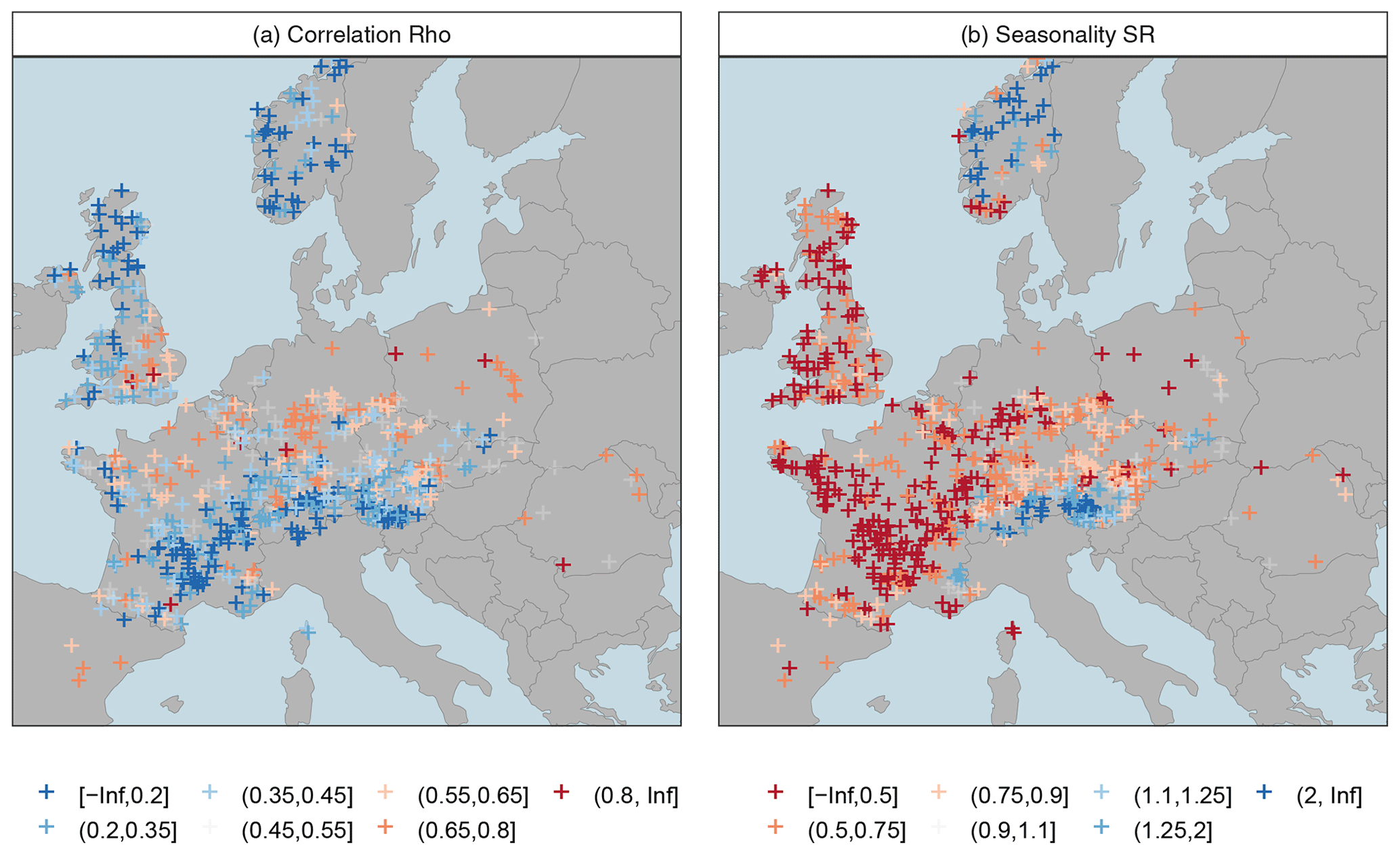
Figure 2Location of gauges and main features of the study: seasonal dependency measured by Spearman's ρ between summer and winter minima series (a) and the seasonality ratio (SR) defined as the ratio of mean winter and mean summer low flow (b).
3.2 Choice of the copula family
As the copula family is a priori unknown, we screened a number of alternative families and compared them using a copula information criterion. Here we used the function xvCopula of the R package copula to compute the cross-validated log likelihood of Grønneberg and Hjort (2014) defined in Eq. (42) therein. When computed for several parametric copula families, it is meaningful to select the family maximizing the criterion. The analyses revealed for the pan-European data set that the Gumbel–Hougaard family performs the best among five extreme value copulas but ranks only slightly above average among eight non-extreme value copula families. In particular, the Gumbel–Hougaard copula (average rank of 5.1) was outperformed by the Plackett copula (average rank 6.5) and the Frank copula (average rank 6.4). As the three models have a contrasting structure and the true model structure is a priori unknown, it was decided to use the station-wide best-fitting model of the three models for the pan-European assessment. In addition, we used the independence copula to model 30 cases with a negative ρ, which was insignificant in all cases. Among the considered models, the Plackett and Frank families are both superior in 308 and 241 cases, while the Gumbel–Hougaard family fits best in 200 cases. Once the family was selected for a station, its parameter θ was fitted using the maximum-likelihood estimator. The resulting copula was finally inserted in the mixed copula estimator (Eq. 6).
3.3 Evaluation method
A similar procedure as in the companion paper is used for model evaluation, which is briefly described below. Again, we assume that the mixed copula estimator is superior to the simpler models, since it is a valid generalization of the annual and the mixed probability estimator (Sect. 2.1). From this point of view, we call the change in performance of the superior model compared to the inferior model a gain in accuracy. However, when we refer to the inferior model, we call the same quantity a loss in accuracy. Note that these deviations are not straightforward errors, since the true distribution is not known, and we can only assume that the model that is more reasonable is also the more accurate one. Based on this terminology, the evaluation is carried out in three analysis steps.
In the first analysis, we assess the performance at the continental scale to learn about the relevance of the enhanced estimator in different regions. The evaluation focuses on the change in return period when using a seasonal probability estimator instead of the conventional annual estimator. This change, or deviation dT of a given return period T, is obtained by calculating the associated flow quantile of the annual estimator and inserting it into the alternative probability distribution. This yields the alternative estimates Tmix when using the mixed distribution approach and TmixC when using the mixed copula estimator. As we are dealing with minima, the return periods are calculated as the reciprocal of the occurrence probability, i.e. .
Consistent with Laaha (2023), the performance gain of the mixed copula estimator over the conventional annual estimator is assessed based on its relative deviation
and its relative absolute deviation (rad)
In the second analysis, we assess the gain of the mixed copula estimator over the mixed probability estimator. For this direct comparison of the two mixed distribution approaches we use their respective deviation
In the third analysis we want to gain deeper insight into the conditions under which the mixed copula approach improves the mixed probability estimator. For this purpose the influencing variables accounting for the difference in both estimators are examined using multiple regression. The predictors considered include the catchment area (AREA), the baseflow index (BFI), and the recession constant as defined in Tallaksen and Van Lanen (2004) and Gustard and Demuth (2008). Because runoff recession in the study area may be disturbed by freezing processes in winter, we chose to use the summer recession constant REC7s based on recession periods of 7 d or more, according to an exploratory assessment.
Table 2Overview of hydrologic predictors used in the regression model.
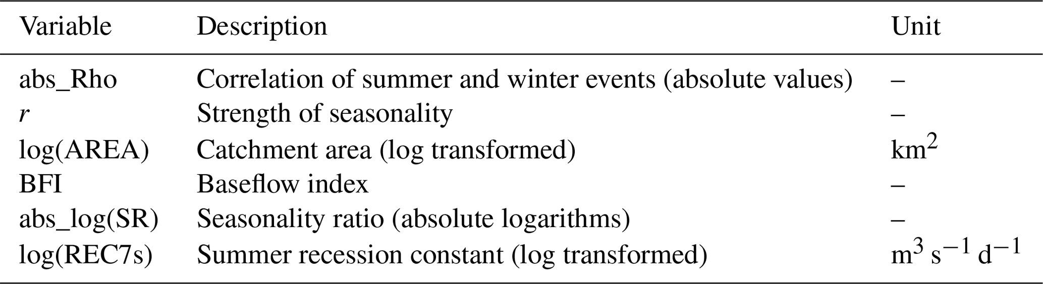
Expecting the estimator to also depend on the strength of seasonality, we include the two seasonality indices described in Sect. 2.3. The SR is calculated as the ratio of the mean summer and winter low flows. Its absolute value thus indicates the strength of seasonality, with values close to 1 corresponding to a perfectly mixed regime and larger values pointing to stronger seasonality. For the index r, a value r=0 indicates that the low flows are equally distributed over the year (weak seasonality) and a value r=1 that all low-flow events fall on the same day of the year (strong seasonality). It has been shown that both indices allow for a good distinction of regime types and can help in identifying characteristic processes as a basis for regionalization (Laaha and Blöschl, 2006). We also considered including a further index, the mixture rate (MR), which indicates the proportion of summer events in the annual minima series (Laaha, 2023). However, as the index performed somewhat worse in a preliminary evaluation, it was not included in the paper.
All predictors have been screened for possible nonlinear correlations using the same procedure as in the companion paper, with a significant difference between linear and rank correlation used as a symptom of nonlinearity. From this preliminary assessment, we have found log-linear relationships of the catchment area and recession constant and decided to use the (decadic) log-transformed variables log(AREA) and log(REC7s) accordingly. For the seasonality ratio we use the absolute logs, termed abs_log(SR), as in the companion paper. Finally, the seasonal correlation is entered as an absolute value (abs_Rho), which appears appropriate to deal with slightly negative correlations observed in a few catchments. The resulting predictors are listed in Table 2.
To test their significance, we use the common Student's t test for regression parameters at the α=0.05 level. We do this using a multiple regression model with main effects and two-way interaction terms. The parameters are checked for collinearity using variance inflation factors (VIFs) and the adjusted coefficient of determination R2. The VIF provides an index that measures how much the variance of an estimated regression coefficient is increased because of collinearity. The adjusted R2 is a penalized measure of model performance so that a greater difference between adjusted and unadjusted R2 will be interpreted as an indication of overfitting and a low difference as an indication of a well-determined model.
The data analysis was performed in R (R Core Team, 2021), using in particular the following packages: lfstat (Gauster et al., 2016), lmom (Hosking, 2022) and FAdist (Aucoin, 2022) for low-flow statistics, drought2015 (internal package by Tobias Gauster), reshape2 (Wickham, 2007), ggplot2 (Wickham, 2016) for drought mapping, copula (Hofert et al., 2022) and VineCopula (Nagler et al., 2022) for copula analysis, and EnvStat (Millard, 2013) and xtable (Dahl et al., 2022) for distribution plots and tables.
4.1 Performance gain compared to the annual estimator
We first assess the performance gain of the mixed copula estimator compared to the annual estimator based on the non-cumulative and cumulative distributions of relative deviances across Europe (Fig. 3). Absolutely large values indicate a big gain of the mixed copula estimator over the conventional frequency analysis approach. Summary statistics of absolute deviations are presented in the upper panel of Table 3. From the graphs, the distribution is quite similar to that of the mixed probability estimator in Austria (Laaha, 2023, Fig. 3). For high return periods such as T=100 years, the spread is somewhat wider than that in the Austrian study, indicating a larger proportion of stations with high deviations. Apart from these extreme cases, 75 % of stations show an (absolute) performance gain of >6 %, 39 % of stations > 50 %, and 25 % of stations > 95.1 %. Minor differences can also be observed for lower return periods, such as the 20-year event, where again 25 % of stations show a performance gain of more than 30.9 %. In fact, we cannot assess at this stage whether the differences are due to the use of a different estimator or a different data set. But overall, the differences between the two studies appear to be small, suggesting a similar performance of both mixed distribution approaches.
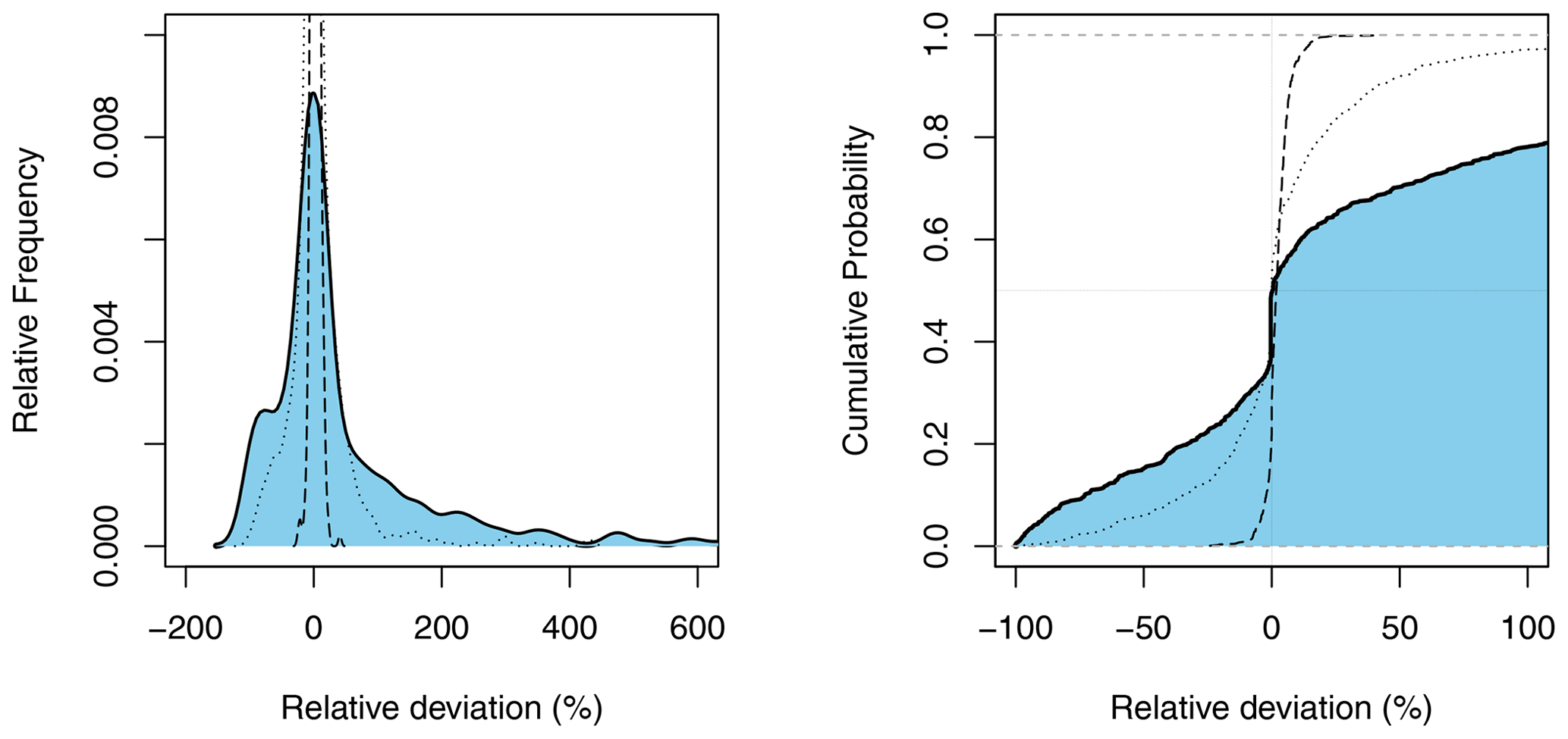
Figure 3Uncertainty of the annual probability estimator compared to the mixed copula estimator. Full line with blue shaded area refers to the 100-year event. For comparison the 20-year event (dotted line) and the 2-year event (dashed line) are shown. Single outliers > 600 % are discarded.
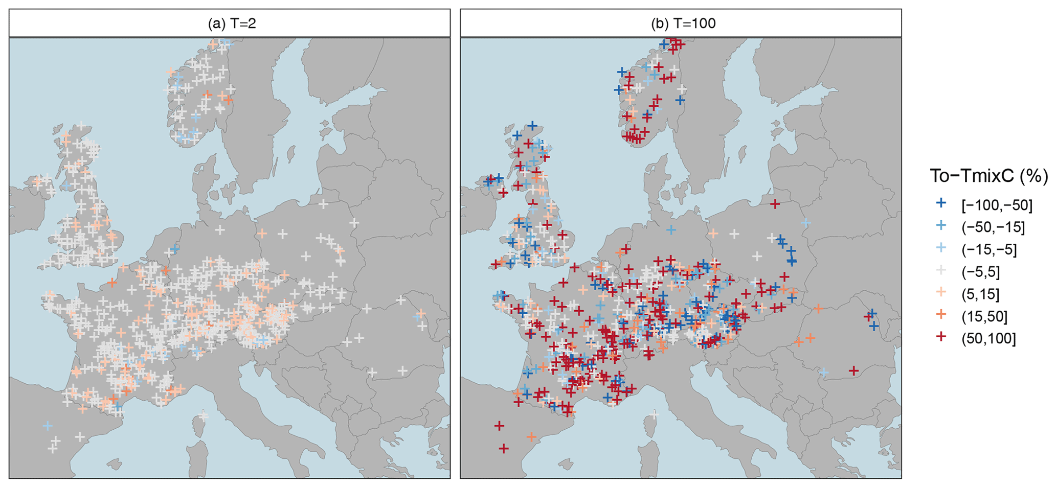
Figure 4Relative deviation (rd) of the mixed copula estimator from the annual probability estimator for a moderate low-flow event with T=2-year return period (a) and an extreme low-flow event with T=100-year return period (b). Blue colours indicate underestimation of the annual probability estimator, the white colour indicates a low difference between estimators, and red colours indicate overestimation of the annual probability estimator.
The companion paper has inferred from the Austrian study area that mixed distribution approaches should be relevant for a wide range of regimes, and it is now interesting to assess this finding at the pan-European scale. Figure 4 shows such a mapping for the relative deviations of the mixed copula estimator for moderate (T=2) and severe (T=100) low-flow conditions and demonstrates that this is indeed the case. Large values are scattered all over Europe, indicating mixture of summer and winter distributions to happen in all regions. For T=100 years the gains (up to 100 %) are most pronounced along the Alpine arch and in Fennoscandia, where the annual estimator often yields higher return periods than the mixed copula approach. Large differences can also be seen in the lowlands north of the Alps where the annual estimator tends to produce lower estimates. For moderate low flows such as the T=2-year event, a different pattern emerges. The gains are generally smaller (mostly up to 10 %, in rare cases up to 40 %), and reddish colours predominate, showing a general tendency of the annual estimator to produce higher estimates. Differences between estimators can be seen in the lowlands north of the Alps, which is subject to cold climate. The deviations tend to be smaller in the west, which is subject to temperate climate. Altogether, the patterns suggest a large gain of the mixed copula estimator, making the method highly relevant for Europe as a whole.
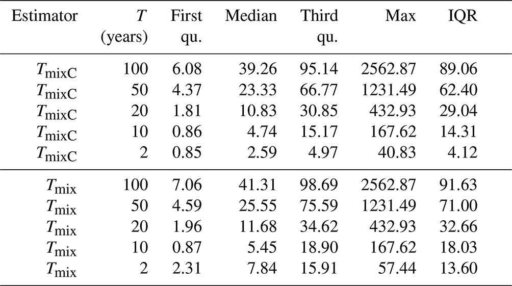
Table 3 allows for a more quantitative assessment. For comparison, the relative absolute deviation of the mixed distribution estimator (Tmix) from Laaha (2023) evaluated for the European data set is presented in the lower panel. The statistics confirm that the two mixed probability estimators, TmixC of this paper and Tmix of the companion paper, actually have quite similar performances. For both estimators, the differences compared to the annual estimator decrease when the return period decreases. This is in line with Laaha (2023), who found that the gain of the mixed probability estimator is substantial at high return periods but diminishes at low return periods. However, the difference between the two estimators increases at low return periods. While the performances are quite similar from 100 to 10 years, the median rad for TmixC and Tmix is 2.59 and 7.84 for T=2 years, respectively. This may point to an interesting difference in the approaches, which will be examined hereafter.
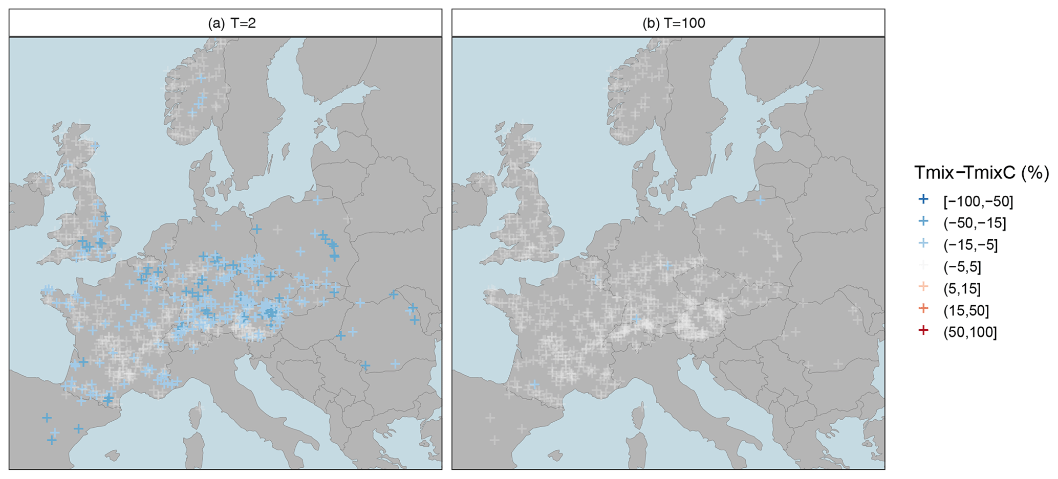
Figure 5Relative deviation Δrd of the mixed copula estimator from the mixed probability estimator for a moderate low-flow event with a T=2-year return period (a) and an extreme low-flow event with a T=100-year return period (b). Blue colours indicate underestimation of the mixed probability estimator, and the white colour indicates a low difference between both estimators.
Table 3Relative absolute deviation (rad) of the mixed copula estimator (TmixC) from the annual probability estimate T (in %). For comparison, the relative absolute deviation of the mixed distribution estimator (Tmix) from Laaha (2023) evaluated for the European data set is presented below. IQR is the interquartile range; the minimum (always 0) is not shown.
4.2 Performance gain compared to the mixed estimator
In the second assessment we evaluate the relative difference in the two mixed distribution approaches in greater detail. Figure 5 and Table 4 show the relative deviations of the mixed copula approach from the mixed probability estimator. As indicated above, the added value of using the copula-based estimator is only minor for the 100-year event. However, the gain for the moderate low-flow event is considerable. Relatively low effects are still observed for western Europe with typical deviations of less than ±5 % in the majority of catchments and between −5 % and −15 % in single catchments. Such low effects are also observed in the high Alps, where the low-flow seasonality is strong and the gain of the mixed estimator was found to be low (Laaha, 2023). Higher differences occur in the northern and southern forelands of the Alps, as well as in central and eastern Europe. In these regions the relative deviation of both estimators are about −15 to −25 %.
Table 4Relative deviation (Δrd) between the mixed and mixed copula probability estimator (%). The maximum values (with exception of four outliers) are always 0 and are therefore not listed in the table.
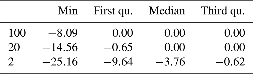
Interestingly, the spatial patterns of Fig. 5a appear quite similar to those of Fig. 4a, suggesting that the difference in the two estimators is generally higher where the gain of the mixed distribution approaches are large. This “size effect” may point to some uncertainty of the mixed probability estimator, which can be corrected using the mixed copula approach. In fact, the difference is always negative or zero (Table 4). Assuming TmixC as the true model, Tmix can be regarded as underestimating the return period and TmixC as correcting this underestimation.
4.3 Conditions that influence the additional performance gain
In a deeper analysis we assess the variables controlling this additional performance gain at low return periods (T=2) by multiple regression. The previous analysis has pointed to a size effect, which is known to predominate in statistical regressions. In order to emphasize the additional effects, a two-step approach is adopted. We first fit a simple linear regression model to adjust for the size effect of the mixed probability estimators, using the relative absolute performance gain of the mixed copula estimator TmixC as a predictor. We then assess the residuals of this model by multiple linear regression with main effects and two-fold interaction terms. Care needs to be taken with regard to the fact that two pairs of predictors, r with SR and BFI with REC7s, are highly correlated, as this may lead to collinear models where parameter estimates and significance values may be incorrect. We therefore fit two alternative models by replacing the two predictors r and BFI in the second model with their correlated alternatives to obtain evidence for all predictors that we consider relevant for this study.
We first analyse the predictors as main effects. This is a simplified assessment as interdependence of the predictors is not covered, and latent interactions may be misclassified as main effects. Nevertheless, the assessment is useful to give the first indication of variables that have some predictive value. The resulting model was carefully checked for overfitting and was found to be well determined. The summary statistics presented in Table 5 show that the three predictors representing seasonal correlation ρ, seasonality r, and baseflow BFI are highly significant, whereas catchment AREA has no significant effect. When we enter the two alternative predictors SR instead of r and REC7s instead BFI, we can see that the seasonality ratio would be significant as well, but no significant effect of the baseflow recession constant could be found. However, the goodness of fit of the first model (R2=0.64) is much higher than for the second model (R2=0.55). The alternative predictors are therefore of little significance for the model.
Table 5Multiple regression summary statistics (main effect model) of the relative deviation (Δrd) between the mixed and mixed copula estimator for the T=2-year return period. The bottom lines show a model alternative where r and BFI were replaced by their correlated counterparts, abs_log(SR) and log(REC7s).
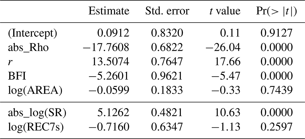
The same procedure was subsequently used to fit a model with main effects and two-fold interaction terms. Care had to be taken for possible overfitting, as the full model had high VIF values (up to 59) for all predictors. The model was therefore subjected to a stepwise variable elimination, which reduced the model by most of the insignificant predictors, thereby resulting in VIFs that were considered acceptable. As the fit improved and overall significances did not change, we found the full model well justified. The model has an R2 of 0.74 and an adjusted R2 of the same value, which also suggests no overfitting and that it is well suited to capture the main differences between the two probability estimators. The summary statistics of the model are shown in Table 6. Interestingly, the model only uses the seasonal low-flow correlation (ρ) as a main effect, which is well in line with the basic intention of the approach to improve the estimation in the case of correlation. The strength of seasonality (r) and catchment storage (BFI) exhibit significant interactions with the seasonal correlation, whereas the catchment area is again not significant. The bottom lines of the table show two model alternatives where r and BFI were replaced by their correlated counterparts, SR and REC7s. Both variables are also significant predictors of seasonality and storage, although in the case of SR with reduced model performance. The analysis suggests that the performance gain of the mixed copula over the mixed distribution estimator can be explained well by the seasonal correlation and catchment characteristics. The model is thus a suitable tool to analyse these effects in more detail.
Table 6Multiple regression summary statistics (main effects and two-way interaction term model) of relative deviation (Δrd) between the mixed and mixed copula estimators for a return period of T=2 years. Insignificant effects were removed by automatic backward stepwise variable selection. The bottom lines show two model alternatives where either r or BFI were replaced by their correlated counterparts, abs_log(SR) (resulting in an R2 of 0.61) and log(REC7s) (R2 of 0.74), respectively.
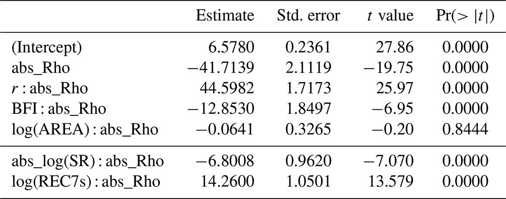
Figure 6 depicts the effects of the considered predictors as partial regression lines together with standard errors and partial residuals. The plots allow a direct comparison of effect size between predictors with various ranges of variability. The results show how much the loss in performance of the mixed probability estimator at low return periods can be attributed to seasonal correlation. Catchments with strong seasonal correlation generally show a stronger underestimation of the mixed probability estimator compared to the copula-based estimator than weakly correlated catchments (Fig. 6a). We interpret this as indicating that the copula estimator effectively reduces the deficiency of the mixed probability estimator caused by correlation of summer and winter events as one would actually expect. However, the correlation effect is modulated by interactions with seasonality and storage (Fig. 6b and c). On the one hand, the tendency to lower estimates is less pronounced for catchments with strong seasonality, where the gain of the mixed estimator was found to be low (Laaha, 2023). This is indicated by a clear positive partial effect of r (Fig. 6b). On the other hand, the correlation effect is enhanced for catchments with a high discharge share from stored sources (such as groundwater, lakes, soil water, or snow storage), as shown by the negative partial effect of the BFI (Fig. 6c). Figure 6d finally reflects our findings above that catchment area has indeed no effect on the performance of the estimator. These results complement the findings from the exemplary catchments of Fig. 1 and generalize them to a wide range of European regimes.
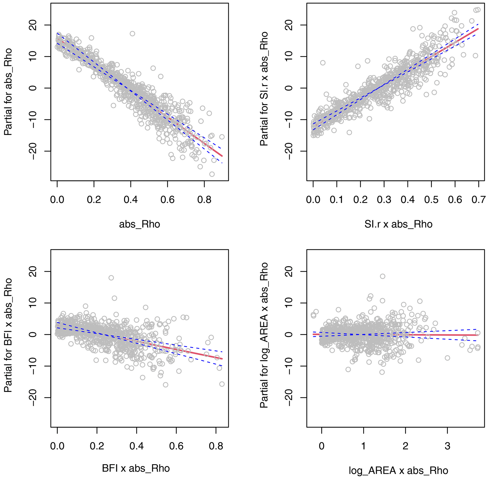
Figure 6Term plot of multiple regression (main effects and two-way interaction term model) of relative deviation (Δrd) between the mixed and mixed copula estimators for a return period of T=2 years.
It is interesting, finally, to assess the spatial patterns of the effects at the pan-European scale (Fig. 7). The upper panels nicely illustrate the antagonistic nature of seasonal correlation and the strength of low-flow seasonality as outlined above. Catchments north of the Alps are prone to strong seasonal correlation, which contributes to an underperformance of Tmix. This affects the mixed low-flow distribution, unless there is strong seasonality as well, so that only one distribution dominates. Such strong (summer) seasonality is typical for temperate climate in western Europe, where the gain of the mixed copula estimator is consequently small (Fig. 5a). The combination of strong correlation and strong summer seasonality corresponds to Type (c) in Fig. 1. However, in regions with weaker seasonality, a stronger mixture of distributions can be observed (Laaha, 2023). Under such conditions, a strong seasonal correlation has a strong effect on the mixed distribution estimator, and the gain of the mixed copula estimator is correspondingly high. Such a constellation typically occurs in mid-mountain regions north of the Alps (e.g. Bavaria and the Ore Mountains – GER, the Tatra Mountains – SLO, Carparthians – PL, and the foothills of the Pyrenees in southern France). The combination of strong correlation and weak to moderate summer seasonality corresponds to Type (b) of Fig. 1, for which a Bavarian gauge is the showcased example. Finally, the lower panels of Fig. 7 depict the interactions between the baseflow index and catchment area, which show much lower effects. Clearly, these variables have a lower contribution to the underperformance of the Tmix. The BFI shows some similarity with seasonal correlation and therefore enhances the correlation effect on the estimator. The AREA, however, shows very small values and should have little impact on the performance of the mixed probability estimator.
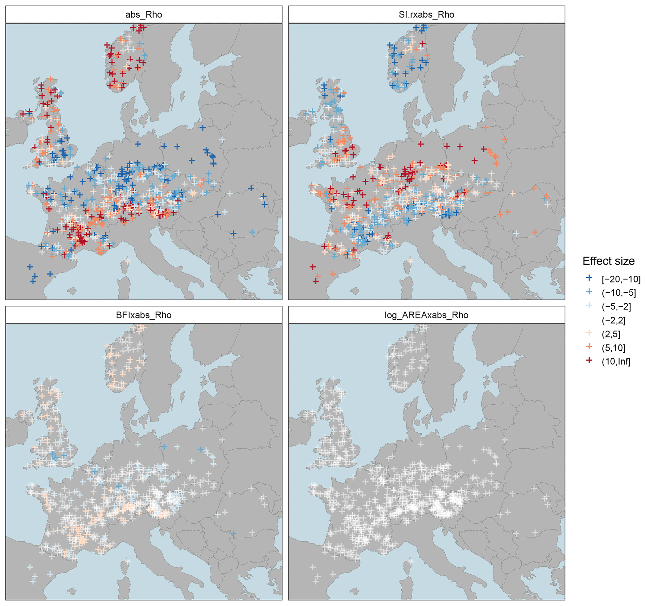
Figure 7Effect size of multiple regression (main effects and two-way interaction term model) of relative deviation (Δrd) between the mixed and mixed copula estimators for a return period of T=2 years.
This second paper of a two-part series presents the mixed copula estimator for low-flow frequency analysis. The method provides an extension of the mixed distribution approach of the companion paper (Laaha, 2023) to deal with the dependency of seasonal events. The paper formulates the copula-based estimator for seasonal minima series and examines its statistical properties in a hydrological context. We carried out a detailed assessment of the method to show its performance compared to the mixed distribution approach.
As a starting point, the distributional characteristics of the mixed copula estimator were assessed by frequency plots of archetypal examples representing contrasting low-flow regimes. Differences in the mixed estimator were always observed in the upper part of the distribution, which, however, is less relevant for low-flow frequency analysis. At severe low-flow events, the differences are very small. For mild to moderate events that fall between these cases, the differences between the two mixed distribution approaches are determined by the interaction between seasonality and seasonal correlation.
In the subsequent step, the performance gain was evaluated based on a larger pan-European data set. The patterns match well with the findings from the exemplary catchments. There is generally little difference between the mixed distribution approaches for severe low-flow events. However, for mild low-flow events the differences are large. For the T=2-year event, the gains of the mixed copula approach are most pronounced in the lowlands north of the Alps, which is subject to cold climate. The gains are much smaller in the west, which is subject to temperate climate. Altogether, the patterns suggest a large gain of the mixed copula estimator over the annual probability estimator, making the method highly relevant for Europe as a whole. Similar effects can be expected around the world in cold and temperate climates, where both summer low flows (due to precipitation deficit) and winter low flows (due to freezing) occur. The method, however, should be less relevant for other (seasonal or aseasonal) climates without a frost season, as generating processes are not so fundamentally different for the low-flow events there.
We then assessed the performance gain of the mixed copula approach over the mixed distribution approach in greater detail. The analysis shows that the gain for the T=100-year event is indeed minimal. However, the gain for mild events is considerable in some of the catchments, with relative deviation of −15 % to −25 % in the most affected regions. The differences increase when the performance gain of the mixed over the annual estimator increases. This points to a size effect that can be interpreted as some inherent uncertainty of the mixed probability estimator, which is corrected by accounting for seasonal correlation. In fact, the differences are always negative or zero so that Tmix shows the tendency to produce lower estimates than TmixC.
Multiple regression analysis suggests that the performance gain of the mixed copula over the mixed distribution estimator can be well explained by the seasonal correlation and catchment-related characteristics. We can interpret the model such that the copula estimator is indeed effective in reducing the underperformance of the mixed probability estimator caused by seasonal correlation. However, the impact of this correlation (and thus the potential of the mixed copula estimator to improve the estimate) is modulated by interactions with seasonality and storage. Effect maps show the strong antagonistic nature of seasonality and seasonal correlation at the European scale, with weak seasonality leading to a high potential for correction and strong seasonal correlation reinforcing the need to take this potential into account. These results are well in line with findings from the exemplary catchments and generalize them to a wide range of European regimes. Storage and catchment size only have a minor effect on the performance gain of the mixed copula estimator and appear to play a subordinate role. This should also be the case for other catchment characteristics, such as soil properties, vegetation, and terrain, which tend to have more influence on surface processes and fast components of the water balance than on long-term storage and thus less influence on the redistribution of water over time.
Although the differences found are high on relative terms, they mostly occur at low return periods. This raises the question of whether it is practical to use the more complex copula-based estimator or whether the simpler mixed distribution approach will suffice. Some indications were already given in the Results section, where regions with large differences and hence a stronger correction were identified. These relate to mid-mountain regions in cold and temperate climates where rivers have strongly mixed low-flow regimes. In these regions, the use of the mixed copula estimator always appears to be beneficial.
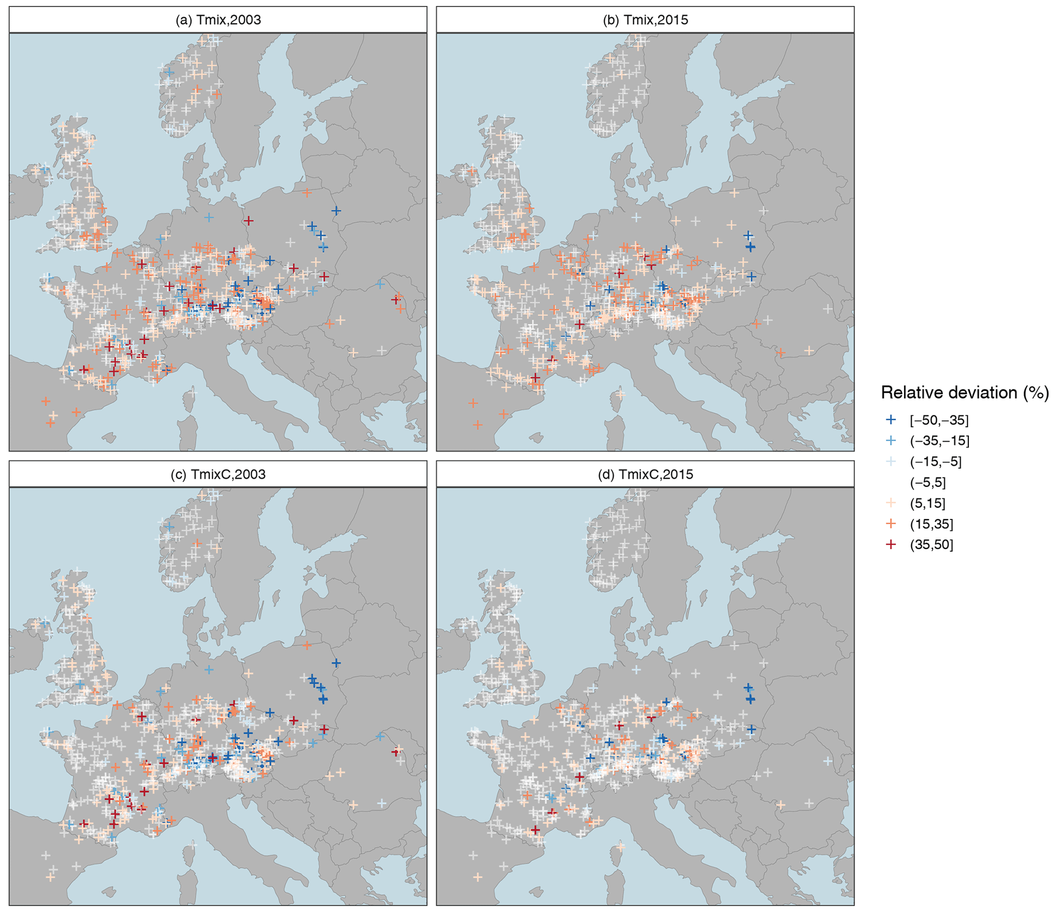
Figure 8Implications of estimation uncertainty for drought event mapping, illustrated for the European cases of 2003 (a, c) and 2015 (b, d). Shown are the relative deviations (rds) of the mixed probability estimator (a, b) and the mixed copula estimator (c, d) from the conventional annual estimate.
Another aspect of practical relevance is the impact of uncertainties on a Europe-wide drought mapping, which is essential for the assessment of major events. Such mapping is often based on return periods that are traditionally obtained by the annual minima approach. This was also the case in our own study of the European drought of 2015 (Laaha et al., 2017). The magnitude of inherent estimation uncertainties with respect to the two enhanced estimators can be seen in Fig. 8. The panels depict the relative deviations of the mixed probability estimator (upper panels) and the mixed copula estimator (lower panels), as compared to the annual estimates for the European 2003 and 2015 cases. Two interesting aspects can be observed. First, the effect of using a mixed probability estimator is again greater the more severe the spatial event. This is suggested by the comparison of the 2003 and 2015 cases, with the event of 2003 having a greater spatial extent and severity. Second, the relative deviations of Tmix are much larger than that of the mixed copula estimator TmixC. This is due to our finding that the Tmix adjusts for the uncertainties of the annual estimator in a number of catchments but appears to underestimate mild drought events. The mixed copula estimator reduces this underestimation in most of these cases, and the correction is particularly visible in regions where a strong seasonal correlation with weak seasonality is superimposed. This suggests that the mixed distribution approaches can indeed be relevant for drought mapping, with the mixed copula approach providing the most accurate estimate.
Despite all the favourable features of the mixed copula estimator, it should be emphasized again that the difference between the two mixed distribution approaches is not large and mainly concerns the low return periods. It is therefore unlikely that severe events in their entirety, i.e. in terms of their spatial extent and severity, will be misclassified by the mixture distribution estimator. Differences are more likely at the regional level where drought conditions may be overlooked. Such regional view, however, is vital for drought monitoring, where the statistically more reasonable concept of the mixed copula estimator should allow for a more accurate assessment of drought severity.
Overall, we conclude that the two mixed probability estimators are quite similar, and both are conceptually more adequate than the annual minima approach. In regions with strong seasonal correlation, the mixed copula estimator appears most appropriate and should be preferred over the mixed distribution approach.
Details on streamflow data collection are given in the cited source: Laaha et al. (2017). Most data are available from the Global Runoff Data Centre portal https://portal.grdc.bafg.de (GRDC, 2022), which contains the former FRIEND European Water Archive. The code will be made available in an updated version of the R software package lfstat via the CRAN repository (R Core Team, 2021).
The author has declared that there are no competing interests.
Publisher's note: Copernicus Publications remains neutral with regard to jurisdictional claims in published maps and institutional affiliations.
Data provision by the Hydrographical Service of Austria (HZB) was highly appreciated. I am grateful to Tobias Gauster for providing a dedicated R environment for European drought mapping. This research is a contribution to the UNESCO IHP-VIII FRIEND-Water programme. I would like to thank the editor and two reviewers for their valuable comments on the manuscript.
This research has been supported by the Climate and Energy Fund under the programme ACRP (grant no. C265154).
This paper was edited by Manuela Irene Brunner and reviewed by Poulomi Ganguli and one anonymous referee.
Ahmadi, F., Radmaneh, F., Sharifi, M. R., and Mirabbasi, R.: Bivariate frequency analysis of low flow using copula functions (case study: Dez River Basin, Iran), Environ. Earth Sci., 77, 1–16, 2018. a
Ahn, K.-H. and Palmer, R. N.: Use of a nonstationary copula to predict future bivariate low flow frequency in the Connecticut river basin, Hydrol. Process., 30, 3518–3532, 2016. a
Ashkar, F., Jabi, N. E., and Issa, M.: A bivariate analysis of the volume and duration of low-flow events, Stoch. Hydrol. Hydraul., 12, 97–116, 1998. a
Aucoin, F.: FAdist: Distributions that are Sometimes Used in Hydrology, R package version 2.4, CRAN [code], https://CRAN.R-project.org/package=FAdist (last access: 13 October 2022), 2022. a
Dahl, D. B., Scott, D., Roosen, C., Magnusson, A., and Swinton, J.: xtable: Export Tables to LaTeX or HTML, R package version 1.8-4, CRAN [code], https://CRAN.R-project.org/package=xtable (last access: 13 October 2022), 2022. a
Fischer, S. and Schumann, A. H.: Multivariate Flood frequency analysis in large river basins considering tributary impacts and flood types, Water Resour. Res., 57, e2020WR029029, https://doi.org/10.1029/2020WR029029, 2021. a
Ganguli, P. and Reddy, M. J.: Risk Assessment of Droughts in Gujarat Using Bivariate Copulas, Water Resour. Manage., 26, 3301–3327, https://doi.org/10.1007/s11269-012-0073-6, 2012. a
Ganguli, P. and Reddy, M. J.: Ensemble prediction of regional droughts using climate inputs and the SVM-copula approach, Hydrol. Process., 28, 4989–5009, https://doi.org/10.1002/hyp.9966, 2014. a
Gauster, T., Laaha, G., and Koffler, D.: lfstat – calculation of low flow statistics for daily stream flow data, R package version 0.9.12, CRAN [code], https://CRAN.R-project.org/package=lfstat (last access: 8 November 2022), 2016. a
Genest, C. and Favre, A.-C.: Everything you always wanted to know about copula modeling but were afraid to ask, J. Hydrol. Eng., 12, 347–368, 2007. a
GRDC: River discharge data portal – Global Runoff Data Centre, Koblenz, Germany, https://portal.grdc.bafg.de (last access: 13 October 2022), 2022. a
Grønneberg, S. and Hjort, N. L.: The Copula Information Criteria: The copula information criteria, Scand. J. Stat., 41, 436–459, https://doi.org/10.1111/sjos.12042, 2014. a, b
Gumbel, E. J.: Distributions des valeurs extremes en plusiers dimensions, Publ. Inst. Statist. Univ. Paris, 9, 171–173, 1960. a
Gustard, A. and Demuth, S.: Manual on low-flow estimation and prediction, in: vol. 50 of Open Hydrology Report, World Meteorological Organization, Geneva, ISBN 978-92-63-11029-9, 2008. a
Hofert, M., Kojadinovic, I., Maechler, M., and Yan, J.: copula: Multivariate Dependence with Copulas, R package version 1.1-0, CRAN [code], https://CRAN.R-project.org/package=copula (last access: 13 October 2022), 2022. a
Hosking, J. R. M.: L-Moments, R package version 2.9, CRAN [code], https://CRAN.R-project.org/package=lmom (last access: 13 October 2022), 2022. a
Jiang, C., Xiong, L., Xu, C.-Y., and Guo, S.: Bivariate frequency analysis of nonstationary low-flow series based on the time-varying copula, Hydrol. Process., 29, 1521–1534, publisher: Wiley Online Library, 2015. a
Klein, B., Schumann, A. H., and Pahlow, M.: Copulas – new risk assessment methodology for dam safety, in: Flood risk assessment and management, edited by: Schumann, A. H., Springer, 149–185, ISBN 978-90-481-9916-7, 2011. a, b, c, d
Laaha, G.: A mixed distribution approach for low-flow frequency analysis – Part 1: Concept, performance, and effect of seasonality, Hydrol. Earth Syst. Sci., 27, 689–701, https://doi.org/10.5194/hess-27-689-2023, 2023. a, b, c, d, e, f, g, h, i, j, k, l, m, n, o, p
Laaha, G. and Blöschl, G.: Seasonality indices for regionalizing low flows, Hydrol. Process., 20, 3851–3878, https://doi.org/10.1002/hyp.6161, 2006. a
Laaha, G., Gauster, T., Tallaksen, L. M., Vidal, J.-P., Stahl, K., Prudhomme, C., Heudorfer, B., Vlnas, R., Ionita, M., Van Lanen, H. A. J., Adler, M.-J., Caillouet, L., Delus, C., Fendekova, M., Gailliez, S., Hannaford, J., Kingston, D., Van Loon, A. F., Mediero, L., Osuch, M., Romanowicz, R., Sauquet, E., Stagge, J. H., and Wong, W. K.: The European 2015 drought from a hydrological perspective, Hydrol. Earth Syst. Sci., 21, 3001–3024, https://doi.org/10.5194/hess-21-3001-2017, 2017. a, b, c, d
Millard, S. P.: EnvStats: An R Package for Environmental Statistics, Springer, New York, ISBN 978-1-4614-8455-4, 2013. a
Nagler, T., Schepsmeier, U., Stoeber, J., Brechmann, E. C., Graeler, B., Erhardt, T., Almeida, C., Min, A., Czado, C., Hofmann, M., et al.: VineCopula: Statistical Inference of Vine Copulas, R package version 2.4.4, CRAN [code], https://CRAN.R-project.org/package=VineCopula (last access: 13 October 2022), 2022. a
Poulin, A., Huard, D., Favre, A.-C., and Pugin, S.: Importance of tail dependence in bivariate frequency analysis, J. Hydrol. Eng., 12, 394–403, 2007. a
R Core Team: R: A Language and Environment for Statistical Computing, R Foundation for Statistical Computing, Vienna, Austria, https://www.R-project.org/ (last access: 13 October 2022), 2021. a, b
Renard, B. and Lang, M.: Use of a Gaussian copula for multivariate extreme value analysis: Some case studies in hydrology, Adv. Water Resour., 30, 897–912, https://doi.org/10.1016/j.advwatres.2006.08.001, 2007. a
Sahoo, B. B., Jha, R., Singh, A., and Kumar, D.: Bivariate low flow return period analysis in the Mahanadi River basin, India using copula, Int. J. River Basin Manage., 18, 107–116, 2020. a
Sklar, M.: Fonctions de repartition an dimensions et leurs marges, Publ. Inst. Stat. Univ. Paris., 8, 220–231, 1959. a
Stahl, K. and Hisdal, H.: Hydroclimatology, in: Hydrological Drought–Processes and Estimation Methods for Streamflow and Groundwater, vol. 48 of Developments in Water Sciences, edited by: Tallaksen, L. M. and Van Lanen, H. A. J., Elsevir, 19–51, ISBN 978-0-444-51688-6, 2004. a
Stahl, K., Vidal, J.-P., Hannaford, J., Tijdeman, E., Laaha, G., Gauster, T., and Tallaksen, L. M.: The challenges of hydrological drought definition, quantification and communication: an interdisciplinary perspective, Proc. IAHS, 383, 291–295, https://doi.org/10.5194/piahs-383-291-2020, 2020. a
Stedinger, J. R., Vogel, R. M., and Foufoula-Georgiou, E.: Frequency analysis of extreme events, in: chap. 18 in Handbook of Hydrology, edited by: Maidment, D. R., McGraw-Hill, ISBN 13:9780070397323, 1993. a
Tallaksen, L. M. and Van Lanen, H. A. J. (Eds.): Hydrological drought: processes and estimation methods for streamflow and groundwater, in: vol. 48 of Developments in Water Sciences, Elsevier, ISBN 978-0-444-51688-6, 2004. a
Van Loon, A. F., Ploum, S. W., Parajka, J., Fleig, A. K., Garnier, E., Laaha, G., and Van Lanen, H. A. J.: Hydrological drought types in cold climates: quantitative analysis of causing factors and qualitative survey of impacts, Hydrol. Earth Syst. Sci., 19, 1993–2016, https://doi.org/10.5194/hess-19-1993-2015, 2015. a
Wickham, H.: Reshaping Data with the reshape Package, J. Stat. Softw., 21, 1–20, 2007. a
Wickham, H.: ggplot2: Elegant Graphics for Data Analysis, Springer-Verlag, New York, ISBN 978-3-319-24277-4, 2016. a
Yue, S., Ouarda, T., Bobée, B., Legendre, P., and Bruneau, P.: The Gumbel mixed model for flood frequency analysis, J. Hydrol., 226, 88–100, https://doi.org/10.1016/S0022-1694(99)00168-7, 1999. a