the Creative Commons Attribution 4.0 License.
the Creative Commons Attribution 4.0 License.
 | 25 May 2023
Why do our rainfall–runoff models keep underestimating the peak flows?
András Bárdossy
Faizan Anwar
In this paper, the question of how the interpolation of precipitation in space by using various spatial gauge densities affects the rainfall–runoff model discharge if all other input variables are kept constant is investigated. The main focus was on the peak flows. This was done by using a physically based model as the reference with a reconstructed spatially variable precipitation model and a conceptual model calibrated to match the reference model's output as closely as possible. Both models were run with distributed and lumped inputs. Results showed that all considered interpolation methods resulted in the underestimation of the total precipitation volume and that the underestimation was directly proportional to the precipitation amount. More importantly, the underestimation of peaks was very severe for low observation densities and disappeared only for very high-density precipitation observation networks. This result was confirmed by using observed precipitation with different observation densities. Model runoffs showed worse performance for their highest discharges. Using lumped inputs for the models showed deteriorating performance for peak flows as well, even when using simulated precipitation.
- Article
(2757 KB) - Full-text XML
- BibTeX
- EndNote


Hydrology is to a very large extent driven by precipitation, which is highly variable in space and time. Point precipitation is interpolated in space that is subsequently used as the true precipitation input for hydrological models without any further adjustments. A common problem with most interpolation schemes is that the variance in an interpolated field is always lower than the variance in the individual point data that were used to interpolate it. Another problem, which is very important in the case of high precipitation events, is that the absolute maximum precipitation coordinates in the interpolated field are at one of the observation locations. Contrary to reality, it is very unlikely that for any given precipitation event the maximum precipitation takes place at any of the observation locations. Accounting for conditional changes with additional variables helps only a little, but it is never enough. New interpolation schemes are introduced on a regular basis, but the main drawback is inherent to all of them. Furthermore, the distribution of the interpolated values tends to be Gaussian, with an increase in the number of observations used for interpolation for each grid cell, even when it is known that the precipitation has an exponential-like distribution in space for a given time step and also for a point in time. From experience in previous studies (Bárdossy et al., 2020, 2022; Bárdossy and Das, 2008), it was clear that model performance was dependent on the number and the configuration of observation station locations, but no decisive conclusion was made. It should not come as a surprise that models perform better, in terms of cause and effect, with increasing data quantity and quality.
1.1 The problem of fewer precipitation observations
The effects of taking a sample from a population on the final distribution of precipitation can be visualized in the following manner. Suppose that precipitation is measured at each point in space. For any given time step, when it is raining at some of the points, the distribution of values is exponential-like. When sampling a finite number of N values from the space, the chances that the points are sampled from the upper tail become smaller and smaller as N approaches 1, or conversely, samples from the lower tail are more likely. This has a strong bearing on the rainfall–runoff process. A large part of small rainfall volumes is intercepted by the soil and the vegetation. These do not influence the peak flows directly. Large flows in rivers are due to soil saturation during or after a rainfall event. To produce soil saturation and therefore runoff, a model first needs to be fed such large precipitation values. The saturation overflow is not necessarily catchment-wide. It could also be due to a large precipitation event over part of the catchment. If the precipitation observation network is not dense enough, then it is possible that a representative pattern of the event is not captured, even after interpolation, due to the reasons mentioned before. Using this false precipitation as model input will consequently lead to producing less saturation overflow and thereby model runoffs not matching the observed.
1.2 Objectives
To investigate the effects of sampling finite points in space on model performance and the reproduction of flood peaks, this study tries to answer the following questions:
-
How strong is the effect of the sampling density on the estimation of areal precipitation for intense precipitation events? Is there a systematic signal?
-
How do interpolation quality and hydrological model performance change with precipitation observation density?
-
How strong is the effect of an error in the precipitation observations on discharge estimations?
-
What is the role of spatial variability in hydrological model performance? How much information is lost if areal mean precipitation is used (i.e., sub-scale variability is ignored)?
Some of the aforementioned points, among others, were recently discussed in a review paper by Moges et al. (2021). They highlighted four sources of hydrological model uncertainties, namely parameter, input, structural, and calibration data uncertainty. Their conclusion was that, out of the four, parameter uncertainty received the most attention, even though all of these sources contribute to the final results in their own unique manner.
Kavetski et al. (2003) concluded that addressing all types of uncertainty will force fundamental shifts in the model calibration/verification philosophy. So far, the rainfall–runoff modeling community has not been able to put such ideas into common practice. The reason for this is that a true estimate of the uncertainty in a forever-changing system is extremely difficult to find. The so-called epistemic uncertainty will always exist. Moreover, there is no consensus on how to model these uncertainties. Following Kavetski et al. (2003), Renard et al. (2010) showed that taking both input and structural uncertainty into account is an ill-posed problem, as combinations of both affect the output and the performance of the model and addressing both simultaneously is not possible.
Balin et al. (2010) tried to assess the impacts of having point rainfall uncertainty on the model discharge by taking a 100 km2 catchment at a spatial resolution of 200 m at a daily timescale. A normally distributed error of 10 % was added to the observed time series to produce a new time series. This was done multiple times and independently. By running the model with the erroneous data (among other things), they found that the resulting performances were not so different from the original case. The only noticeable difference was that the uncertainty bounds on discharge were slightly wider, resulting in more observed values being contained by it. The conclusion was that the causes of model output uncertainty may not be due to erroneous data, as the measurement errors everywhere compensated for the runoff error in a way that the final model performance stayed the same. More interestingly, they found out that using observed rainfall for modeling resulted in the underestimation of the peak flows, a problem that this study will also try to address. Furthermore, for the same catchment, Lee et al. (2010) arrived at similar conclusions by using a different approach and a lumped rainfall–runoff model. Yatheendradas et al. (2008) investigated the uncertainty of flash floods using a physically based distributed model by considering a mixture of parameter and input data uncertainty. They concluded that their model responses were heavily dependent on the properties of the precipitation estimates using radar, among other findings.
This study is a special case of model input uncertainty. It specifically deals with the effects of using interpolated precipitation data as a rainfall–runoff model input that is derived from point observations. It does not deal with input uncertainty as it is meant to be, as doing so requires very strong assumptions that are likely to remain unfulfilled (as was also pointed out in Beven, 2021). The idea that various forms of uncertainties exist and should be considered is not disputed.
The rest of the study is organized as follows. Section 2 shows the investigation area, and Sect. 3 shows the model setup, inputs, and the main idea of this study in detail. Section 4 discusses the two rainfall–runoff models used in this study and the methods of their calibration. Section 5 discusses the results in detail, where the questions posed in the beginning of this section are answered. Section 6 presents two coarse correction approaches that were tried to reduce precipitation bias. Finally, in Sect. 7, the study ends with the summary, main findings, and implications of the results.
The study area is the Neckar catchment situated in the southwest of Germany in the federal state of Baden-Württemberg (Fig. 1). It has a total area of 14 000 km2. In the east, it is bounded by the Swabian Alps and by the Black Forest in the west. The maximum elevation is ca. 1000 m in the Swabian Alps that goes down to 170 m at the confluence of the Neckar and Rhine in the north. Mean recorded temperature is about 9.1 ∘C, while the minimum and maximum temperatures ever recorded are −28.5 and 40.2 ∘C, respectively. Annual precipitation sums reach about 1800 mm in the Black Forest, while the rest of the area receives mean precipitation of 700 to 1000 mm. The probability of precipitation on a given day and at a specific location is ca. 50 %, with a mean precipitation of 2.5 mm d−1.
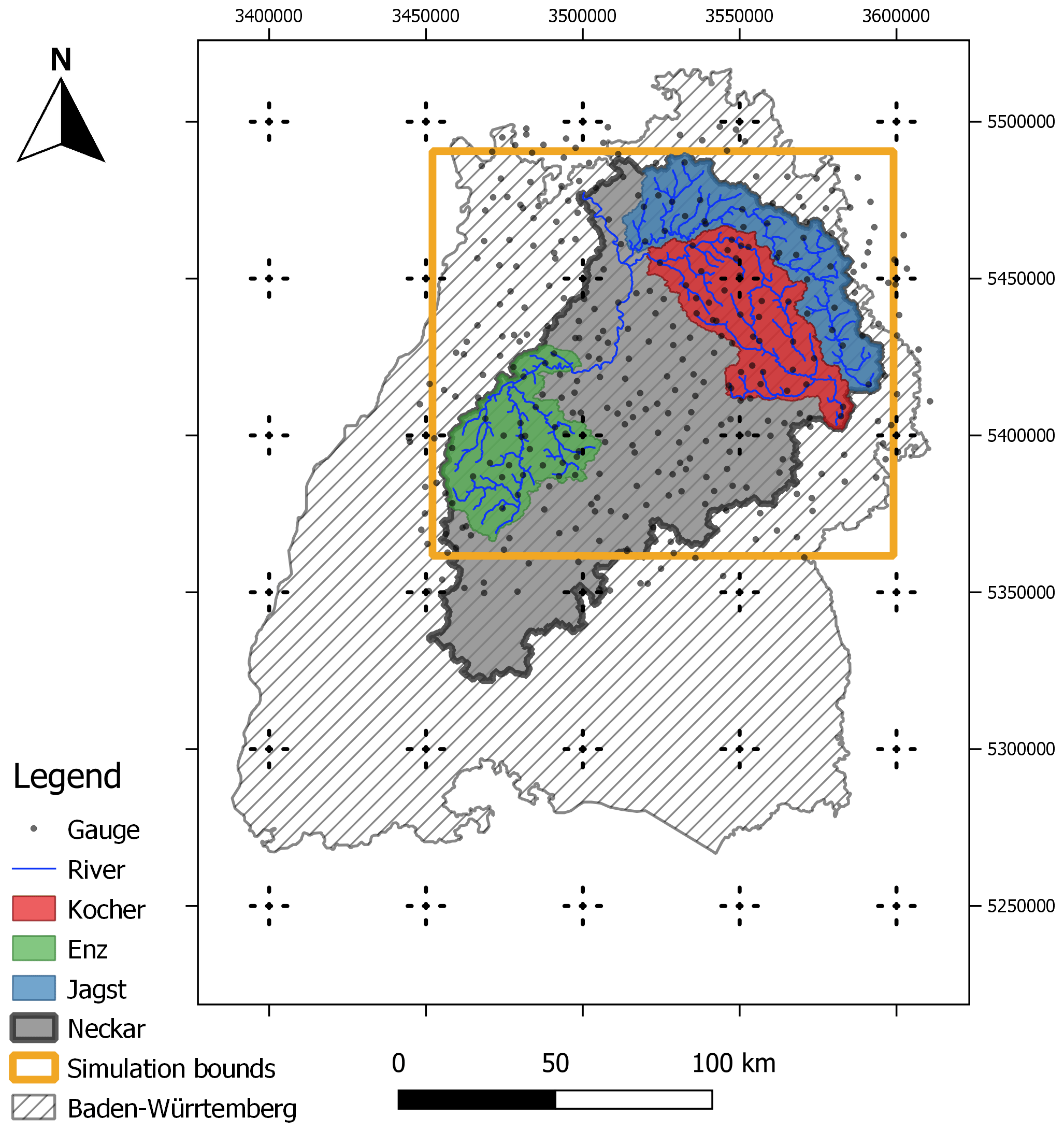
Figure 1Study area (taken from Bárdossy et al., 2022).
The entire catchment area of the Neckar was not modeled by the considered rainfall–runoff models in this study. Rather, the large headwater catchments were modeled only where the times of the concentration were long enough to allow for model runs on a daily resolution (i.e., if a large precipitation event takes place, then the ensuing peak in discharge is observed at the next time step). The Enz, Kocher and Jagst, with catchment areas of 1656, 1943, and 1820 km2, respectively, were studied. Other reasons for the selection of these catchments were that they are relatively intact compared to the main river, which is modified for transportation, and also the fact the effects of catchment boundaries (e.g., exact boundary line and exchanges with neighboring catchments) vanish as the size becomes larger.
Point meteorological data time series (daily precipitation and temperature) were downloaded from the Deutscher Wetter Dienst (DWD; German Weather Service) open-access portal (DWD, 2019). The daily discharge time series was downloaded from the open-access portal of the Landesanstalt für Umwelt Baden-Württemberg (LUBW; Environmental Agency of the Federal State of Baden-Württemberg; LUBW, 2020). The considered time period is from 1991 to 2015. Furthermore, the precipitation gauges used in this study are evenly distributed across the catchment, even at high elevations (Fig. 2). This is very important because one of the cited causes of precipitation volumes (e.g., Yang et al., 1999; Legates and Willmott, 1990; Neff, 1977) is the smaller density of gauges at higher elevations. It is also important to note that effects of elevation on daily precipitation are negligible (Bárdossy and Pegram, 2013).

Figure 2Comparison of elevation distributions of observation locations (red) and the whole simulation grid (blue) using the Shuttle Radar Topography Mission (SRTM) 90 m grid for the study area.
3.1 Precipitation interpolation using various gauge densities
To demonstrate the effects of various gauge densities on the peak flows of the models, time series of the existing precipitation network for the time period of 1991–2015 were taken. There were a total of 343 gauges. Only a subset of these was active at any given time step, as old stations were decommissioned and new ones were commissioned. Out of the total, random samples sized 10, 25, 50, and 100, 150 gauge time series were selected, and gridded precipitation was interpolated using these for each catchment that was subsequently lumped into a single value for each time step. This was done 100 times. For comparison, the same was done by using all the gauges. Furthermore, two interpolation schemes, namely nearest neighbor (NN) and ordinary kriging (OK), were used to show that the problem was not interpolation scheme dependent. A stable variogram fitting method that was described in Bárdossy et al. (2021) was used for OK.
3.2 Reference precipitation
In the previous case, precipitation interpolations were not compared to reality, as one cannot not know what the real precipitation was at locations with no stations. To obtain a complete coverage of rainfall, simulated precipitation fields were considered.
A realistic virtual dataset was created to investigate the effect of the precipitation observation density instead of using interpolated precipitation. For this purpose, a 25-year-long daily precipitation dataset corresponding to the time period of 1991–2015 was used. This dataset contains gridded precipitation on a 147×130 km grid with 1 km resolution. It was created so that the precipitation amounts were the same as the observed precipitation at the locations of the weather service observation stations. Additionally, the empirical distribution function of the entire field for any selected day is the same as that of the observations, and its spatial variability (measured as the variogram) is the same as the observed. This precipitation is considered to be reality. It is called the reference or reconstructed precipitation throughout this text. Full details of the procedure are described in Bárdossy et al. (2022). To summarize the idea of the said study, consider the problem of inverse modeling in which a physically based rainfall–runoff model is set up for a catchment. Daily fields of interpolated precipitation are fed to it, among other inputs. The model hydrograph is computed. It should come as no surprise that the model and observed runoff do not match. Assume that all the errors in the model hydrograph are due to precipitation only. Now the question to be answered is as follows: what precipitation will result in a hydrograph that has very little to no error compared to the observed? To find the answer, new realizations of precipitation that are constrained to have precipitation values that are exactly the same as those at the observation locations, along with the same correlation function for any given time step in space, are needed. The time step with a large error is selected, and precipitation fields for the about 10 time steps before this are simulated and fed to the model as new inputs. The resulting error is checked. If it reduces, then the new precipitation fields replace the old ones as observed. If not, then they are rejected, and new ones are simulated and tested. This procedure is repeated up to the point where the model runoff error stops improving. Next, another time step is selected that is far away (more than 10 time steps) from the one rectified before, and the same procedure is repeated for that one. In this way, all the time steps are treated and a new time series of precipitation fields is obtained that has significantly fewer errors compared to the case when interpolated precipitation is used.
3.3 Precipitation interpolation using the reference
To demonstrate the effects of the sparse sampling of data and the resulting model runoff error, the following method was used.
N number of points were sampled from the reference grid. A time series for each point (1×1 km cell) was then extracted and taken as if it were an observed time series. Care was taken to sample points such that the density was nearly uniform over the study area. N was varied to obtain a given amount of gauge density. Here, densities of 1 in 750, 400, 200, and 130 km2 were used. These correspond to 25, 50, 100, and 150 cells out of the 19 110, respectively. Labels of the form MN are used to refer to these in the figures, where M is a suffix to signify interpolation, and N being the number of points used to create the interpolation. For reference, Germany has around 2000 active daily precipitation stations for an area of 360 000 km2, which is about one station per 180 km2. The random sampling was performed 10 times for each N in order to see the effects of different configurations later on in the analysis of the results.
In this way, many time series were sampled from the reference for various gauge densities. From here on, the same procedure was applied that is normally used in practice (i.e., spatial interpolation). To keep things simple, the OK method was used to interpolate fields on the same spatial resolution as the reference at each time step. The use of OK is arbitrary. One could just as well use any preferred method. The use of other methods that interpolate in space will not help much, as all of them tend to result in fields that have reduced variance as compared to the variance of the observed values. Moreover, it is also very unlikely (but possible in theory) that an interpolation scheme predicts an extreme at locations where no measurements were made.
3.4 Temperature and potential evapotranspiration
External drift kriging (EDK; Ahmed and De Marsily, 1987) was used to interpolate the daily observed minimum, mean, and maximum temperature for all cells at a resolution similar to that of the precipitation with resampled elevation from the Shuttle Radar Topography Mission (SRTM; Farr et al., 2007) dataset as the drift. For potential evapotranspiration (PET), the Hargreaves–Samani (Hargreaves and Samani, 1982) equation was used with the interpolated temperature data at each cell as input. It was assumed that temperature and potential evapotranspiration are much more continuous in space as compared to precipitation, which behaves as a semi-Markov process in space–time that has a much larger effect on the hydrograph in the short term. To clarify that the role of temperature and PET is not very important while considering peaks, consider the following: peaks are a result of large-scale precipitation. It could be due to continuous precipitation that is not very intense but persists longer in time or an intense event of a smaller duration. Long precipitation events result in very little sunlight and therefore little evapotranspiration. What is the effect of 2 mm of evapotranspiration on a day where it rained 50 mm? An intense event will result in the saturation of the soil and increased overland flow, which is again not enough time for evapotranspiration to have any significant impact. The only time when temperature may have a considerable effect is when it becomes very low, a large snow event takes place for many days, and then the temperature suddenly rises rather quickly in the coming days (it is very rare). For example, such an event that is on record in the study area took place in 1882. This was also investigated previously in Bárdossy et al. (2020). Even then, the effect of temperature is modeled to a very good extent by the interpolation, due to its nature in space–time.
Two rainfall–runoff models, namely SHETRAN (Ewen et al., 2000) and HBV (Bergström, 1992), were considered in this study. The same gridded inputs were used for both at a spatial resolution of 1×1 km and at a daily temporal resolution. Except for precipitation, all other inputs remained the same during all the experiments. A description of the model used and the setup specific to each is discussed in the following two subsections.
4.1 SHETRAN
SHETRAN is a physically based distributed hydrological model which simulates the major flows (including subsurface) and their interactions on a fine spatial grid (Ewen et al., 2000). It includes the components for vegetation interception and transpiration, overland flow, variably saturated subsurface flow and channel–aquifer interactions. The corresponding partial differential equations are solved using a finite difference approximation. The model parameters were not calibrated. Instead, available data, such as the elevation, soil, and land use maps were used to estimate the model parameters at a 1×1 km spatial resolution (Lewis et al., 2018; Birkinshaw et al., 2010). It was considered to be a theoretically correct transformation of rainfall to runoff. In this way, combined with the reference precipitation, a realistic virtual reality was created in which the effect of different sampling densities could be investigated. Same SHETRAN settings were used for the various precipitation interpolations. Furthermore, the model and settings are the same as those in Bárdossy et al. (2022), which the readers are encouraged to read before proceeding further.
4.2 HBV
HBV is one of the most widely used models that needs no introduction. It requires very little input data (i.e., precipitation, temperature, and potential evapotranspiration). Each grid cell of HBV was assumed to be a completely independent unit. All cells shared the same parameters, and only the inputs were different. The runoff produced by all cells was summed up at the end to produce the final simulated discharge value for each time step. It was calibrated for the reference precipitation and each of the precipitation interpolation steps. Differential evolution (DE; Storn and Price, 1997) was used to find the best parameter vector. It is one of the genetic-type optimization schemes to find the global optimum by updating a given sample of parameter vectors successively by mixing three in a specific manner. A population size of 400 was used to find the global optimum. Overall, it needed 150 to 200 iterations to converge for 11 parameters. In total, 50 % Nash–Sutcliffe (NS; Nash and Sutcliffe, 1970) and 50 % NS using the natural logarithm (Ln-NS) was used as the objective function for calibration. Ln-NS was chosen because NS alone concentrates too much on the peak flows during calibration and disregards almost 95 % of the remaining flows. Ln-NS helps to mitigate this flaw to some degree but not completely.
Before showing the results, some terms specific to the following discussion are defined first. They are put here for the readers' convenience.
-
The term reference precipitation refers to the reconstructed precipitation that is taken as if it were the observation. The term reference model refers to SHETRAN, with the reference precipitation as input and the resulting discharge of this setup is the reference discharge.
-
The term interpolated discharge refers to the discharge of SHETRAN or HBV with interpolated precipitation as input. The model is mentioned specifically for this purpose. The term subsampling refers to extraction of the time series of a subset of points from the entire grid.
-
The term model performance refers to the value of the objective function whose maximum, and optimum, value is 1.0; anything less is a poorer performance. The performance of the reference discharge is 1.
-
Furthermore, the terms discharge and runoff are used interchangeably. They both refer to the volume of water produced by a catchment per unit of time, which is cubic meters per second in this study. The terms observation station, gauge, and station are used interchangeably. These refer to the meteorological/discharge observation stations.
5.1 Metrics used for evaluation
To compare the change in precipitation or model runoff, scatterplots of the reference values on the horizontal versus their corresponding values after interpolation on the vertical scale are shown. Each point represents the lumped precipitation for all the cells (i.e., mean of all the cells per time step).
The largest five aerially lumped values for precipitation in the reference and the values at the corresponding time steps in interpolation are compared by showing them as a percentage of the reference. This produces a number of points that is the product of the number of interpolations and the considered number of events. For comparing discharge, the five largest values in the reference discharge are compared against the values at the same time steps using interpolated discharge. This results in five points per interpolation. Violin plots are used to show these points as densities.
Furthermore, figures comparing a high discharge event using all the interpolations are shown at the end of each subsection, wherever relevant. Tables summarizing the over- and underestimations as percentages relative to the reference are shown at the end of each subsection.
5.2 Comparison of interpolations using fewer vs. all gauges
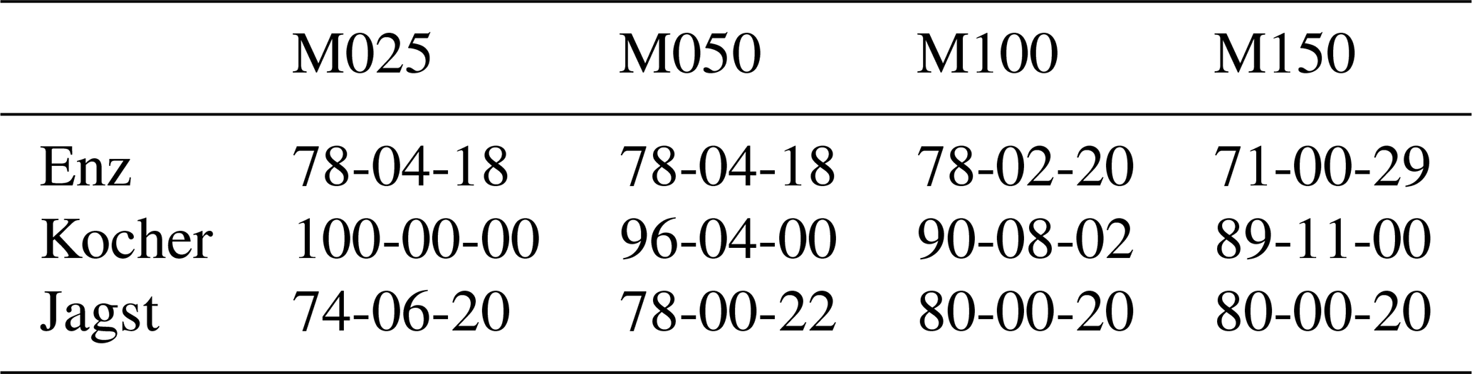
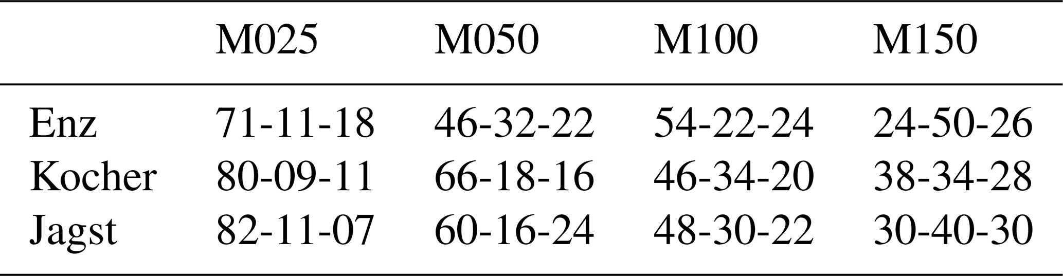
A comparison of the depth of the largest five precipitation events, using various numbers of gauges taken from the entire network, are shown in Figs. 3 and 4 for Enz. These are normalized with respect to the values computed using the entire network (343 gauges). There are many cases in which the fewer gauge interpolations have larger values than the ones making use of the entire network. However, the more important point to notice is the bias. By using a lower number of gauges, an underestimation of the largest precipitation events is more likely. NN exhibits a larger variance in terms of under- and overestimations compared to OK. Using more gauges shows that the deviations reduce significantly. Another aspect that should be kept in mind is that here the interpolations are compared to an interpolation. Even by using all of the gauges, there is still a very high chance of missing the absolute maximum precipitation at a given time step. Keeping this in mind, one should be aware that the runoff predicted by a model using this smoothed precipitation with all the gauges will still produce, on average, smaller peaks. This will become clearer from the results in the next sections, where the reference precipitation is used. Tables 1 and 2 summarize the cases with under- and overestimations, using various numbers of gauges with respect to using all of them for interpolation for the three catchments, using NN and OK, respectively.
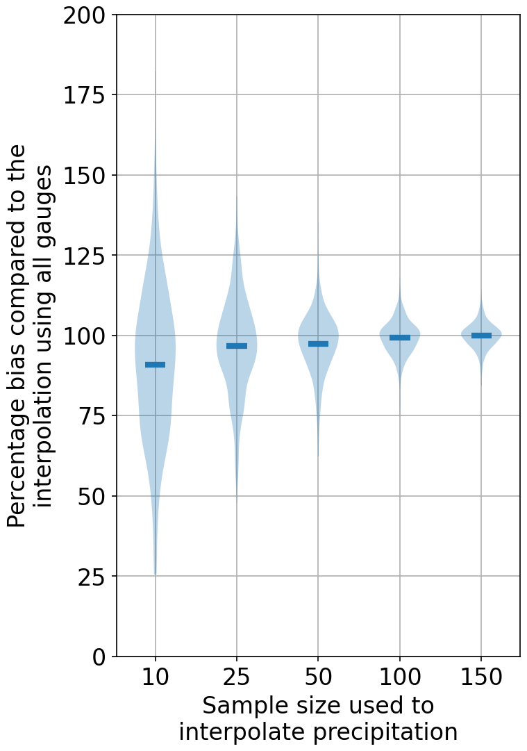
Figure 3Precipitation bias comparison of the top five largest values due to using fewer points against an interpolation that uses all of the points using NN.
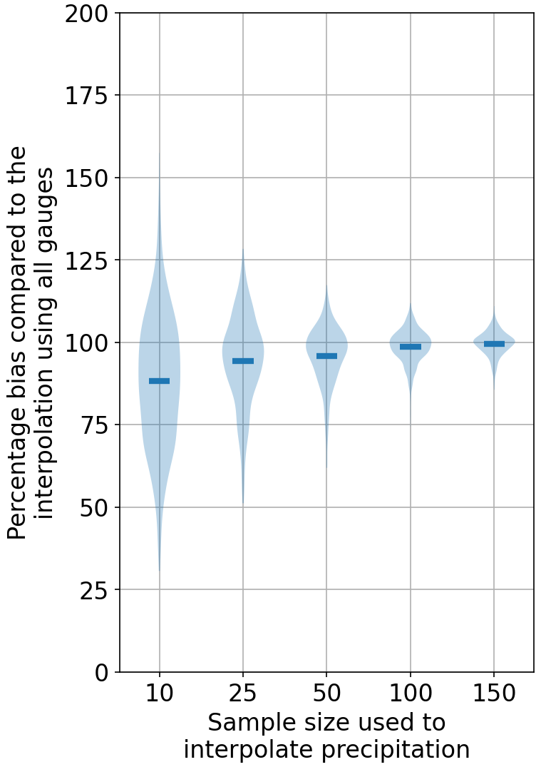
Figure 4Precipitation bias comparison of the top five largest values due to using fewer points against an interpolation that uses all of the points using OK.
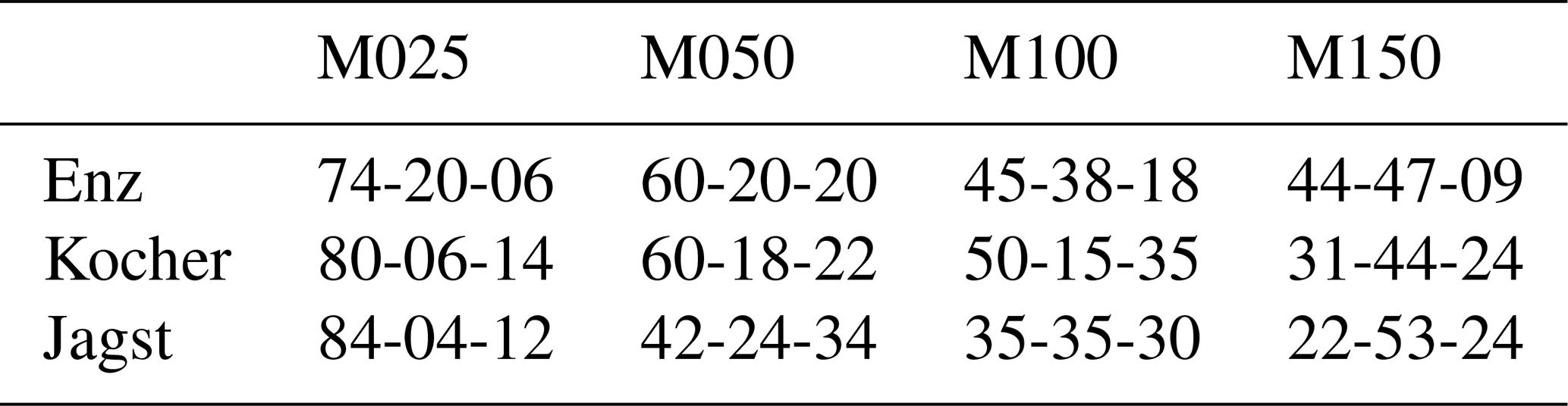
Table 1Relative percentages of under- and overestimations of the top five precipitation events using various gauge densities (columns) with respect to the top five values using interpolation with all of the gauges for the three considered catchments (rows) using NN. The values are of the format of the percentage of underestimations (below 97.5 %), within a threshold of ±2.5 %, and overestimations (above 102.5 %) with respect to the interpolation using all of the gauges. For example, 60-09-31 in the first row and first column means that, out of the 100 interpolations (with five events per interpolation) using 10 gauges for Enz, 60 % of the events were below 97.5 %, 9 % were within 97.5 % and 102.5 %, and 31 % were above 102.5 % of the top five events using the interpolation with all of the 343 gauges.
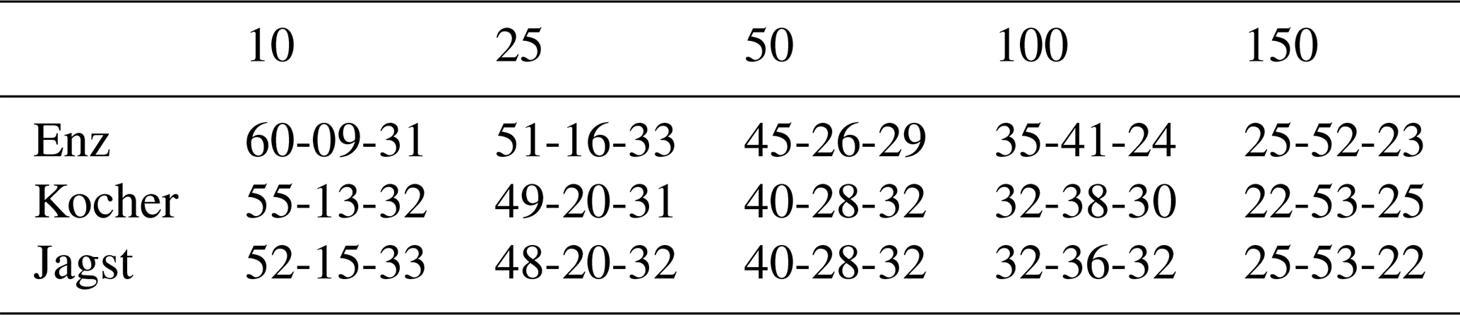
Table 2Under- and overestimation percentages of the top five precipitation events using OK. The caption of Table 1 explains how to interpret the numbers here.

5.3 Effects of subsampling from reference on precipitation
Figure 5 shows an exemplary event with very high daily precipitation for the reference and various interpolation cases. For the lowest number of gauges, the field appears to be very smooth and has a smaller variance compared to the field with the most stations which is much closer to the reference.
In Fig. 6, the scatterplot of the lumped reference against one of the lumped interpolation values for all time steps for Kocher is shown. Here, it is interesting to notice that, overall, the larger the value in reference, the more it is reduced by the interpolation. On the other hand, the interpolation increases the magnitude of the smaller values. Events in the mid-range values are underestimated by a significant margin. Most points are below the ideal line. Consider the subsequent mass balance problems that could arise from such a consistent bias. In the long term, one would adjust the model to have lower evapotranspiration. In the short term, the peak flows would almost always be underestimated. It is important to keep in mind that high discharge values are the result of a threshold process in the catchment where the water moves in larger volumes towards the stream once the soil saturates or when the infiltration cannot keep up with the rainfall/melt intensity. To match the peaks in such scenarios, it is important to obtain the correct estimates of precipitation.

Figure 5Comparison of precipitation interpolations for a time step with high precipitation with the reference.
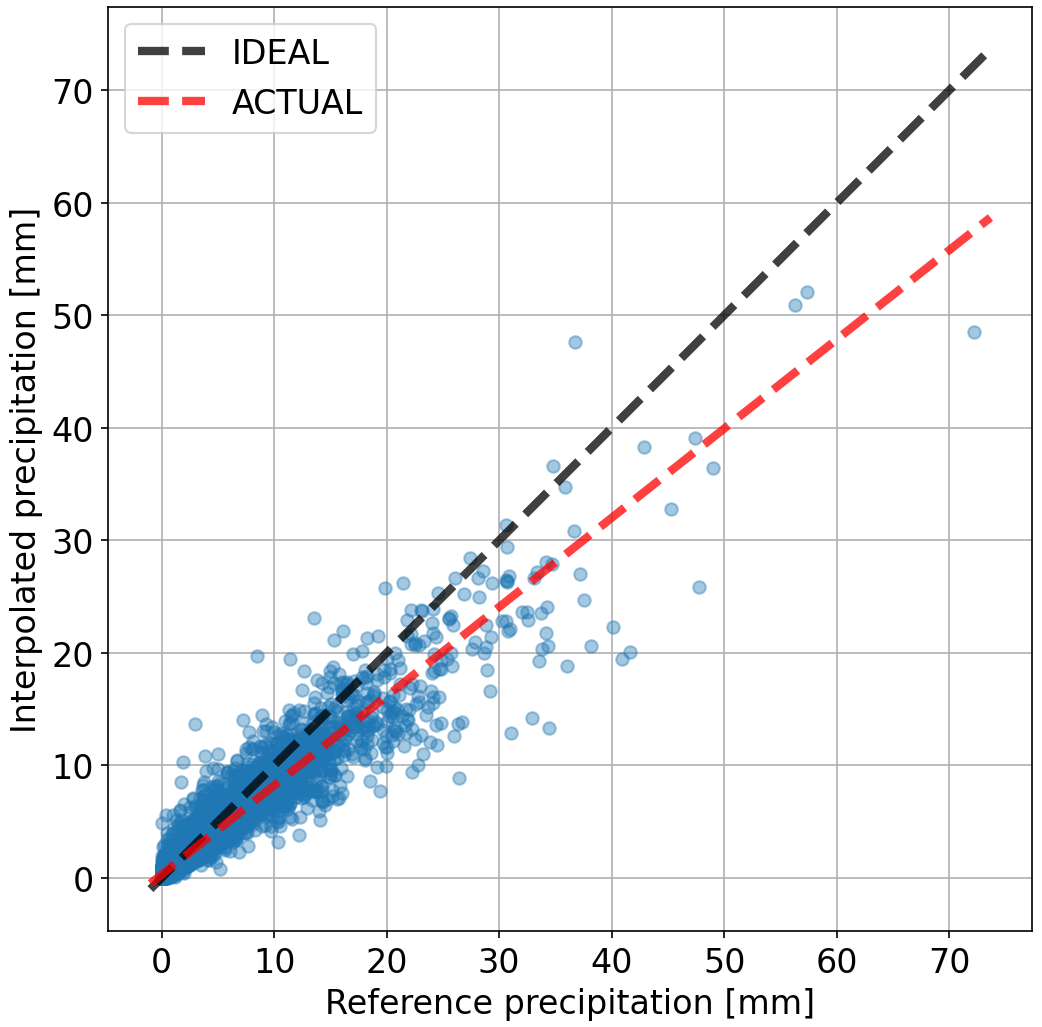
Figure 7 shows the relative change in the largest five peak precipitation values. These were computed by dividing the interpolated precipitation by the reference at the time steps of the top five events. A consistent bias (i.e., underestimation) is clear, especially for the coarsest interpolation (25 points). Such a bias appears small, but consider the extra volume over a 1000 km2 catchment that is not intercepted by the soil. Another interesting point to note is that, for the other interpolations, there are some overestimations as well. All the relative under- and overestimations for the three catchments with various densities are summarized in Table 3.

Figure 7Precipitation bias comparison of various interpolations with respect to the reference for the top five largest values.
Table 3Percentages of under- and overestimations of the top five precipitation events using various gauge densities (columns) with respect to the top five values using reference precipitation for the three considered catchments (rows). The values are of the format of the percentage of underestimations (below 97.5 %), within a threshold of ±2.5 %, and overestimations (above 102.5 %) with respect to the reference precipitation. For example, 31-44-24 in the second row and last column means that, out of the 10 interpolations (with five events per interpolation) using 150 points for Kocher, 31 % of the events were below 97.5 %, 44 % were within 97.5 % and 102.5 %, and 24 % were above 102.5 % of the top five events using the reference precipitation.
5.4 Effects of subsampling from reference on discharge of SHETRAN
Similar to the precipitation, systematic bias in model runoff was investigated next. Figure 8 shows the resulting runoff by using the same precipitation (Fig. 6) as input to SHETRAN. What is immediately clear is that there are almost no overestimations of discharge values when using interpolated precipitation. The largest peak is reduced by almost 50 %.
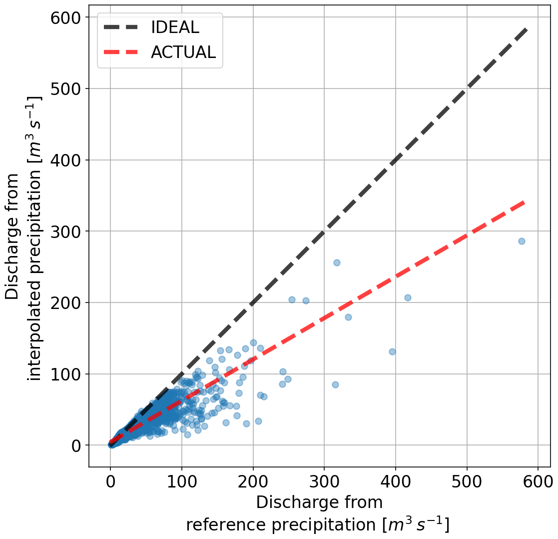
Figure 8Scatter of discharge using reference and interpolated precipitation for one catchment using SHETRAN.
Looking at Fig. 9, the mean of the largest five peaks is reduced significantly while using the least number of points for Kocher. The other point to note is that the peaks drop on average for other interpolations (except for the last one), which is much more compared to the reduction in precipitation. To see the effects more in detail, Figs. 10 and 11 show hydrographs obtained using various gauging densities for two events. It is very clear that, as the gauging density rises, the underestimation decreases proportionally, and the hydrographs become similar. All the under- and overestimations are summarized in the Table 4 for all the catchments.
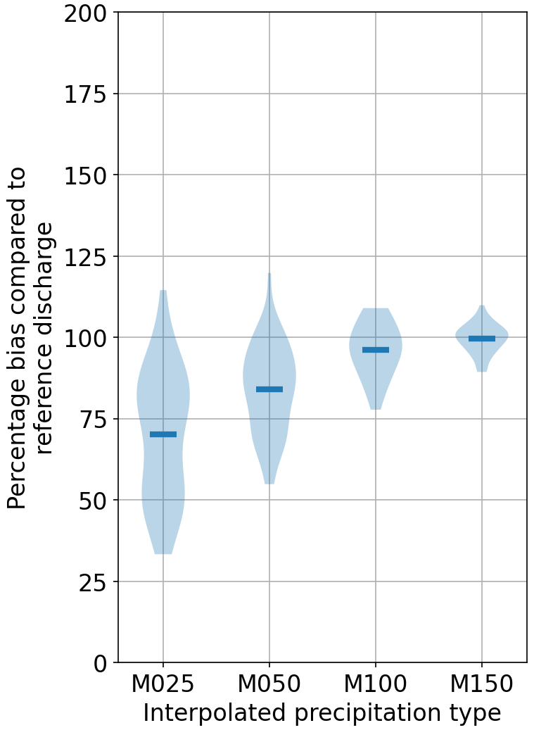
Figure 9Discharge bias comparison of various interpolations with respect to the reference for the top five largest values using SHETRAN.
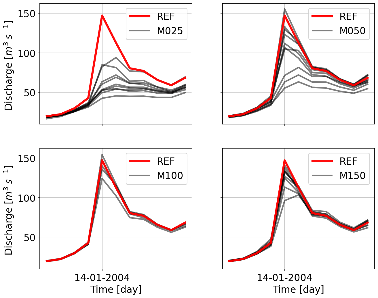
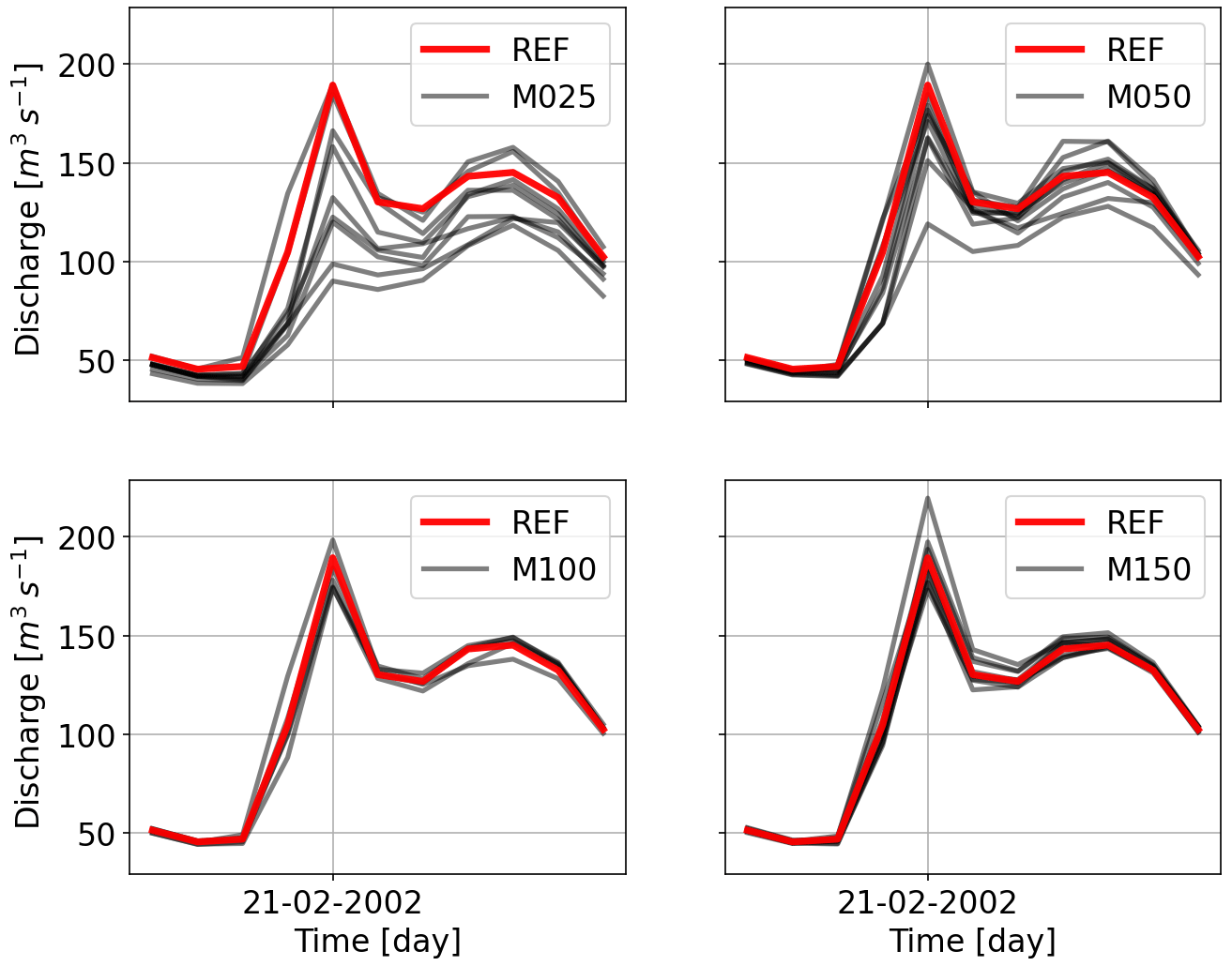
Table 4Percentages of under- and overestimations of the top five discharge events using various gauge densities (columns) with respect to the top five values using reference discharge for the three considered catchments (rows) using SHETRAN. The values are of the format of the percentage of underestimations (below 97.5 %), within a threshold of ±2.5 %, and overestimations (above 102.5 %) with respect to the reference discharge. For example, 38-38-24 in the third row and last column means that, out of the 10 interpolations (with five events per interpolation) using 150 points for Jagst, 38 % of the events were below 38 %, 38 % were within 97.5 % and 102.5 %, and 24 % were above 102.5 % of the top five events using the reference discharge.

5.5 Effects of subsampling from reference on discharge of HBV
While observing the scatter of the reference and interpolated precipitation discharge in Fig. 12, HBV shows a different behavior compared to SHETRAN. Overestimations from low to high flows exist, except for the largest high flows which are underestimated as well, which, again, is not as much as that by SHETRAN. This is due to the recalibration, where the new parameters compensate for the missing precipitation by the decrease in evapotranspiration. This aspect will be investigated thoroughly in future research.
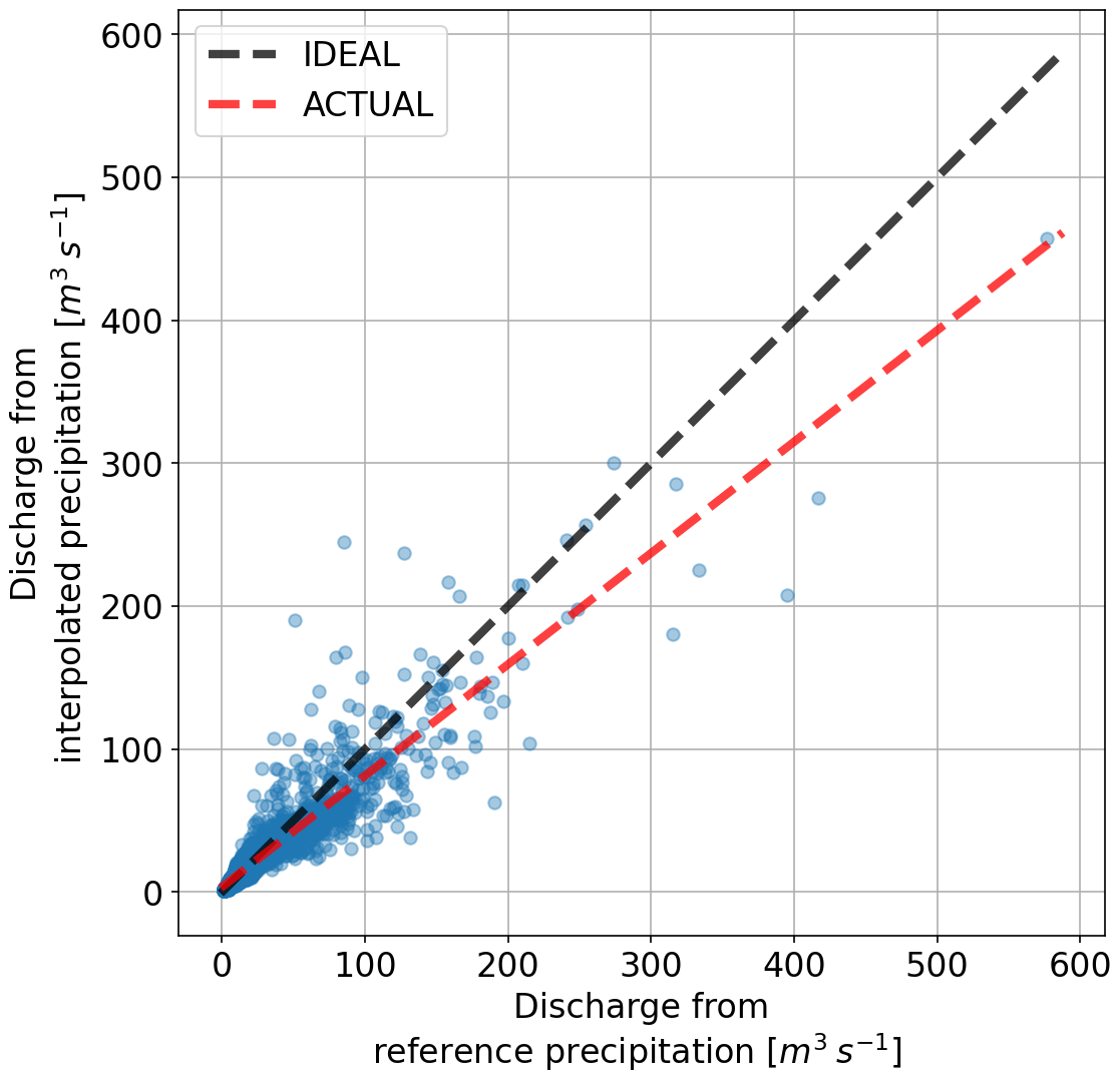
Figure 12Scatter of discharge using reference and interpolated precipitation for one catchment using HBV.

Figure 13Discharge bias comparison of various interpolations with respect to the reference for the top five largest values using HBV.
Figure 13 shows the scaling of the five highest peaks compared to the reference discharge. Here, a similar reduction for the least number of stations can be seen. Even for the highest number of stations, the discharges are still underestimated. This signifies that even a distributed HBV with the full freedom to readjust its parameters cannot fully mimic the dynamics of the flow produced by SHETRAN. Hydrographs for the same events shown in the previous section for HBV are shown in Figs. 14 and 15. It is interesting to note that the first event is overestimated by all the interpolations and that the hydrographs become similar to the gauging density increases. The second event is estimated better as the gauging density increases. All the under- and overestimations are summarized in the Table 5 for all the catchments.
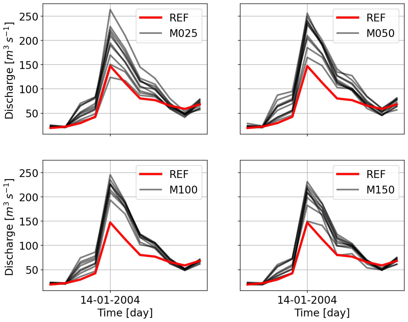
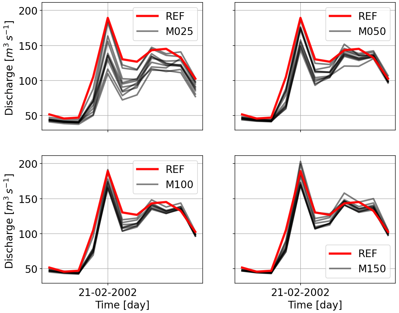
Table 5Percentages of under- and overestimations of the top five discharge events using various gauge densities (columns) with respect to the top five values using reference discharge for the three considered catchments (rows) using HBV. The caption of Table 4 explains how to interpret the numbers here.
5.6 Effects of removing subscale variability in precipitation on SHETRAN discharge
The effects of using lumped precipitation on the resulting discharge (i.e., mean precipitation value at each time step for all cells) were also investigated. The aim was to see the effects of subscale variability on runoff. While considering 10 largest peaks per catchment for the entire time period, the NS efficiencies of these dropped to 0.77, 0.78, and 0.90 for Enz, Kocher, and Jagst respectively. Almost all peaks were reduced in their magnitudes to 84 %, 85 %, and 93 % with respect to the ones produced by the model on average with the distributed reference precipitation. Most of the underestimation of the peaks was during winter, which is likely to be snowmelt events. These are location/elevation dependent, and it makes sense that using a lumped value of precipitation results in incorrect melt behavior. Overall, the tendency was towards reduced discharge when using lumped precipitation. This tendency is likely to be much higher when a single cell is used to represent the catchment (i.e., a fully lumped model).
5.7 Effects of measurement error in precipitation on runoff
To test how the measurement error affects the model discharge, precipitation with a measurement error of 10 % of each observed value having a standard normal distribution was used and then interpolated as well. There, it was observed that the magnitude of the under- and overestimation of the peaks becomes more variable as compared to the reference, but the bias remained the same as that compared to using precipitation with no error. Table 6 shows the effects for precipitation. Comparing these to Table 3, it can be concluded that the trends are not significantly different for the two cases. Similar to interpolations with no errors, the ones with the largest number of samples have more values closer to the reference precipitation. These results corroborate the conclusions by Balin et al. (2010), Lee et al. (2010).
These results have an interesting consequence. If the gauges have measurement errors that are normally distributed, then cheaper gauges, such as the Netatmo personal weather stations, can be used to close the gap of missing precipitation due to sparse distribution networks. Studies, such as those by de Vos et al. (2017), de Vos et al. (2019), and Bárdossy et al. (2021), have shown that these alternative sources of data can augment the existing networks, while still having some drawbacks. The type of measurement error by these can be further studied to validate their usefulness for rainfall–runoff modeling.
Table 6Percentages of under- and overestimations of the top five precipitation events using various gauge densities (columns) with respect to the top five values using reference precipitation for the three considered catchments (rows). The values are of the format of the percentage of underestimations (below 97.5 %), within a threshold of ±2.5 %, and overestimations (above 102.5 %) with respect to the reference precipitation. For example, 38-34-28 in the second row and last column means that, out of the 10 interpolations (with five events per interpolation) using 150 points for Kocher, 38 % of the events were below 97.5 %, 34 % were within 97.5 % and 102.5 %, and 28 % were above 102.5 % of the top five events using the reference precipitation.
Consistent bias was shown by the interpolated precipitation. Consequently, rectifying it was attempted by transforming the precipitation in such a manner that an improvement in the discharge could be observed. Two different approaches were tested. These are described as follows.
Static transform of the form
where ψ is a threshold for transformation. β is a multiplier, while γ is an exponent that may transform the values above the threshold either linearly or nonlinearly.
Using transforms that neither consider the time of the year nor the type of weather during a precipitation event are also not optimal. For example, precipitation events in summer are more intense, occur for a shorter period of time, are more abrupt in nature, and cover smaller areas as compared to winter, where the intensity is less, they occur for longer periods of time, and cover much larger areas. Accounting for such information while correcting for bias can be useful. Hence, transformations based on weather circulation patterns (CPs) were used to correct the precipitation bias based on the type of event. An automatic CP classification method based on fuzzy logic (Bárdossy et al., 2002) was used to find relevant CPs that were dominant in the study area. The procedure assigns a type of weather to each time step based on the atmospheric pressure in and around the catchment area and some other constraints. The number of CPs that may be obtained is arbitrary. For this study, five CPs were chosen based on previous experience and also to avoid too many free variables for calibration. The transformation was then applied to precipitation that took place only in the two CPs that were related to the wettest weather. Contrary to a static transform based on the precipitation magnitude only, independent of time or weather, transforms are applied to each time step based on its CP, which depends on the weather and time of the year. The CP-based transform was as follows:
where βCP is a CP-dependent multiplier, and γCP is a CP-dependent exponent.
Finally, a simple experiment was set up to search for a consistent pattern in the unknown terms of the transforms using the lumped HBV. The method to find the optimal transformation involved applying the same transform to precipitation values for all catchments while optimizing their model parameters independently. The assumption is that the model efficiencies will bring better performance compared to the case where no precipitation correction was considered. This leads to a problem of optimization in higher dimensions. For the previous cases, the optimization of model parameters was carried out for each catchment independently, which was an 11-dimensional problem. For the case of testing transforms, the model parameters of the three catchments and the unknown transform parameters have to be optimized simultaneously. This has to be the case, as optimizing transforms for each catchment will lead to them being very different to the neighbors. However, considering the behavior of precipitation in space, it could be argued that each catchment should be treated individually, but here the aim was to evaluate if an overall correction was possible. Hence, 36 parameters for the static transform case and 37 for the CP-based case had to be optimized. For the case of the static transform, a slight improvement in the results was observed for all the catchments, but no consistent patterns were observed, as was the case for the CP-based case. Strangely, all transforms resulted in a reduction in the high precipitation values, which signifies that the problem of the large precipitation underestimation cannot be considered independently of the low and medium precipitation values. Similar approaches and more sophisticated ones will be investigated in later research.
An often-ignored problem of peak flow underestimation in rainfall–runoff modeling by using interpolated data was investigated in this study. To do so, data were interpolated using different gauge densities. It was shown how interpolated precipitation differs from reference precipitation. This may come as no surprise, as interpolation produces smooth transitions between two or more points that are very unlikely to represent the actual state of the variable in space–time. SHETRAN was used as a reference model that was assumed to represent reality with reconstructed precipitation as input. The other model was HBV. Runoff from SHETRAN was chosen as a reference to avoid an inherent mismatch of mass balances as compared to using the observed discharge series. Simple approaches for bias correction were also presented, where it was learned that the bias cannot be corrected using simple static- or weather-dependent transforms of input precipitation.
We arrived at the following answers to the questions that were stated at the beginning:
-
The sampling density of stations in and around a catchment has profound effects on the quality of interpolated precipitation. While it is obvious that more stations lead to better estimates of precipitation, it was recognized that a low density leads to a more frequent high underestimation of areal precipitation, especially for the large events. Depending on the density, the worst case was an underestimation of about 75 % of the precipitation volume. This effect decreased as the sampling density increased.
-
Both considered hydrological models showed a consequent underestimation of peak flows. For example, SHETRAN produced a peak that was about 50 % less compared to the case when reference precipitation was used. HBV did not show a comparatively similar loss, as it was recalibrated each time for different precipitation, but its performance deteriorated nonetheless.
-
Similar to previous studies, the effects of random measurement errors in precipitation on model discharge were not significant.
-
Using precipitation as input with no spatial variability showed an overall loss in model performance, especially for the events that involved snowmelt.
Further conclusions that can be derived from the abovementioned results are as follows:
-
While modeling in hydrology, variables should be modeled in space and time at the correct resolution to have usable results. Disregarding spatial characteristics (in terms of variance) leads to problems that cannot be solved by any model or finer-resolution temporal data.
-
Cheaper networks may prove valuable where observations are sparse, if the condition that their measurement errors are normally distributed is met.
-
Finally, the results and conclusions of this study must be interpreted with the important fact in mind that models were used to demonstrate the effects of the underestimation of peaks due to sparse networks and interpolations. In reality, it could very well be that these effects become less dominant/observable due to any number of other reasons, such as incorrect temperature or discharge readings, or due to using models that insufficiently represent all the processes the lead to river flows or changes in it. Nevertheless, this study proves that the main culprit behind the underestimation of peaks is the observation network density, provided that a model is used that has a description of the dominant rainfall–runoff-producing mechanisms in it. The models used to demonstrate the effects are circumstantial to a large extent, as the peak flow underestimation is due to the missing volume of input precipitation.
In future research, the following issues could be addressed:
-
The underestimation of intense precipitation due to interpolation.
-
The sensitivity of other variables, such as temperature, to interpolation and their effects on runoff, especially in catchments with seasonal or permanent snow cover.
-
The magnitude of performance compensation that recalibration introduces due to the missing precipitation.
-
The effects of using different density networks on calibrated model parameters and the regionalization of model parameters.
-
The determination of the error distributions of cheaper precipitation gauges to establish their usefulness in rainfall–runoff modeling.
BA: conceptualization and SHETRAN modeling. FA: HBV modeling. BA and FA: data preparation and final preparation of the paper.
At least one of the (co-)authors is a member of the editorial board of Hydrology and Earth System Sciences. The peer-review process was guided by an independent editor, and the authors also have no other competing interests to declare.
Publisher’s note: Copernicus Publications remains neutral with regard to jurisdictional claims in published maps and institutional affiliations.
Python (van Rossum, 1995), NumPy (Harris et al., 2020), SciPy (Virtanen et al., 2020), Matplotlib (Hunter, 2007), pandas (The pandas development team, 2020; Wes McKinney, 2010), pathos (McKerns et al., 2012), PyCharm IDE (https://www.jetbrains.com/pycharm/, last access: 3 July 2019), Eclipse IDE (https://www.eclipse.org/ide/, last access: 26 January 2019), and PyDev (https://www.pydev.org/, last access: 17 February 2019). The authors acknowledge the financial support of the research group FOR 2416 “Space–Time Dynamics of Extreme Floods (SPATE)” by the German Research Foundation (DFG) and the University of Stuttgart for paying the article-processing charges of this publication. Last but not least, we would also like to thank Keith Beven, Alberto Montanari, and the anonymous reviewer for their valuable comments.
This research has been supported by the Deutsche Forschungsgemeinschaft (grant no. FOR 2416 (SPATE)).
This open-access publication was funded by the University of Stuttgart.
This paper was edited by Yue-Ping Xu and reviewed by Keith Beven, Alberto Montanari, and one anonymous referee.
Ahmed, S. and De Marsily, G.: Comparison of geostatistical methods for estimating transmissivity using data on transmissivity and specific capacity, Water Resour. Res., 23, 1717–1737, https://doi.org/10.1029/WR023i009p01717, 1987. a
Balin, D., Lee, H., and Rode, M.: Is point uncertain rainfall likely to have a great impact on distributed complex hydrological modeling?, Water Resour. Res., 46, https://doi.org/10.1029/2009WR007848, 2010. a, b
Bárdossy, A. and Das, T.: Influence of rainfall observation network on model calibration and application, Hydrol. Earth Syst. Sci., 12, 77–89, https://doi.org/10.5194/hess-12-77-2008, 2008. a
Bárdossy, A., Stehlík, J., and Caspary, H.-J.: Automated objective classification of daily circulation patterns for precipitation and temperature downscaling based on optimized fuzzy rules, Clim. Res., 23, 11–22, https://doi.org/10.3354/cr023011, 2002. a
Bárdossy, A., Seidel, J., and El Hachem, A.: The use of personal weather station observations to improve precipitation estimation and interpolation, Hydrol. Earth Syst. Sci., 25, 583–601, https://doi.org/10.5194/hess-25-583-2021, 2021. a
Bergström, S.: The HBV Model: Its Structure and Applications, SMHI Reports Hydrology, SMHI, https://books.google.de/books?id=u7F7mwEACAAJ (last access: 10 February 2021), 1992. a
Beven, K.: An epistemically uncertain walk through the rather fuzzy subject of observation and model uncertainties, Hydrol. Process., 35, e14012, https://doi.org/10.1002/hyp.14012, 2021. a
Birkinshaw, S. J., James, P., and Ewen, J.: Graphical user interface for rapid set-up of SHETRAN physically-based river catchment model, Environ. Modell. Softw., 25, 609–610, 2010. a
Bárdossy, A. and Pegram, G.: Interpolation of precipitation under topographic influence at different time scales, Water Resour. Res., 49, 4545–4565, https://doi.org/10.1002/wrcr.20307, 2013. a
Bárdossy, A., Anwar, F., and Seidel, J.: Hydrological Modelling in Data Sparse Environment: Inverse Modelling of a Historical Flood Event, Water, 12, https://doi.org/10.3390/w12113242, 2020. a, b
Bárdossy, A., Modiri, E., Anwar, F., and Pegram, G.: Gridded daily precipitation data for Iran: A comparison of different methods, J. Hydrol., 38, 100958, https://doi.org/10.1016/j.ejrh.2021.100958, 2021. a
Bárdossy, A., Kilsby, C., Birkinshaw, S., Wang, N., and Anwar, F.: Is Precipitation Responsible for the Most Hydrological Model Uncertainty?, Frontiers in Water, 4, https://doi.org/10.3389/frwa.2022.836554, 2022. a, b, c, d
de Vos, L., Leijnse, H., Overeem, A., and Uijlenhoet, R.: The potential of urban rainfall monitoring with crowdsourced automatic weather stations in Amsterdam, Hydrol. Earth Syst. Sci., 21, 765–777, https://doi.org/10.5194/hess-21-765-2017, 2017. a
de Vos, L. W., Leijnse, H., Overeem, A., and Uijlenhoet, R.: Quality Control for Crowdsourced Personal Weather Stations to Enable Operational Rainfall Monitoring, Geophys. Res. Lett., 46, 8820–8829, https://doi.org/10.1029/2019GL083731, 2019. a
DWD: https://opendata.dwd.de/climate_environment/CDC/observations_germany/climate/daily/ (last access: 25 November 2019), 2019. a, b
Ewen, J., Parkin, G., and O'Connell, P. E.: SHETRAN: distributed river basin flow and transport modeling system, J. Hydrol. Eng., 5, 250–258, 2000. a, b
Farr, T. G., Rosen, P. A., Caro, E., Crippen, R., Duren, R., Hensley, S., Kobrick, M., Paller, M., Rodriguez, E., Roth, L., Seal, D., Shaffer, S., Shimada, J., Umland, J., Werner, M., Oskin, M., Burbank, D., and Alsdorf, D.: The Shuttle Radar Topography Mission, Rev. Geophys., 45, https://doi.org/10.1029/2005RG000183, 2007. a
Hargreaves, G. and Samani, Z.: Estimating potential evapotranspiration, Journal of the Irrigation and Drainage Division, 108, 225–230, 1982. a
Harris, C. R., Millman, K. J., van der Walt, S. J., Gommers, R., Virtanen, P., Cournapeau, D., Wieser, E., Taylor, J., Berg, S., Smith, N. J., Kern, R., Picus, M., Hoyer, S., van Kerkwijk, M. H., Brett, M., Haldane, A., del Río, J. F., Wiebe, M., Peterson, P., Gérard-Marchant, P., Sheppard, K., Reddy, T., Weckesser, W., Abbasi, H., Gohlke, C., and Oliphant, T. E.: Array programming with NumPy, Nature, 585, 357–362, https://doi.org/10.1038/s41586-020-2649-2, 2020. a
Hunter, J. D.: Matplotlib: A 2D graphics environment, Comput. Sci. Eng., 9, 90–95, https://doi.org/10.1109/MCSE.2007.55, 2007. a
Kavetski, D., Franks, S. W., and Kuczera, G.: Confronting Input Uncertainty in Environmental Modelling, pp. 49–68, American Geophysical Union (AGU), 2003. a, b
Lee, H., Balin, D., Shrestha, R. R., and Rode, M.: Streamflow prediction with uncertainty analysis, Weida catchment, Germany, KSCE J. Civ. Eng., 14, 413–420, 2010. a, b
Legates, D. R. and Willmott, C. J.: Mean seasonal and spatial variability in gauge-corrected, global precipitation, Int. J. Climatol., 10, 111–127, https://doi.org/10.1002/joc.3370100202, 1990. a
Lewis, E., Birkinshaw, S., Kilsby, C., and Fowler, H. J.: Development of a system for automated setup of a physically-based, spatially-distributed hydrological model for catchments in Great Britain, Environ. Modell. Softw., 108, 102–110, https://doi.org/10.1016/j.envsoft.2018.07.006, 2018. a
LUBW: https://udo.lubw.baden-wuerttemberg.de/public/ (last access: 16 August 2020), 2020. a, b
McKerns, M. M., Strand, L., Sullivan, T., Fang, A., and Aivazis, M. A.: Building a framework for predictive science, arXiv [preprint], https://doi.org/10.48550/arXiv.1202.1056, 2012. a
Moges, E., Demissie, Y., Larsen, L., and Yassin, F.: Review: Sources of Hydrological Model Uncertainties and Advances in Their Analysis, Water, 13, 28, https://doi.org/10.3390/w13010028, 2021. a
Nash, J. and Sutcliffe, J.: River flow forecasting through conceptual models. 1. A discussion of principles, J. Hydrol., 10, 282–290, 1970. a
Neff, E. L.: How much rain does a rain gage gage?, J. Hydrol., 35, 213–220, https://doi.org/10.1016/0022-1694(77)90001-4, 1977. a
Renard, B., Kavetski, D., Kuczera, G., Thyer, M., and Franks, S. W.: Understanding predictive uncertainty in hydrologic modeling: The challenge of identifying input and structural errors, Water Resour. Res., 46, https://doi.org/10.1029/2009WR008328, 2010. a
Storn, R. and Price, K.: Differential Evolution – A Simple and Efficient Heuristic for global Optimization over Continuous Spaces, J. Global Optim., 11, 341–359, 1997. a
The pandas development team: pandas-dev/pandas: Pandas, Zenodo, https://doi.org/10.5281/zenodo.3509134, 2020. a
van Rossum, G.: Python tutorial, Tech. Rep. CS-R9526, Centrum voor Wiskunde en Informatica (CWI), Amsterdam, https://www.python.org/ (last access: 20 May 2020), 1995. a
Virtanen, P., Gommers, R., Oliphant, T. E., Haberland, M., Reddy, T., Cournapeau, D., Burovski, E., Peterson, P., Weckesser, W., Bright, J., van der Walt, S. J., Brett, M., Wilson, J., Millman, K. J., Mayorov, N., Nelson, A. R. J., Jones, E., Kern, R., Larson, E., Carey, C. J., Polat, İ., Feng, Y., Moore, E. W., VanderPlas, J., Laxalde, D., Perktold, J., Cimrman, R., Henriksen, I., Quintero, E. A., Harris, C. R., Archibald, A. M., Ribeiro, A. H., Pedregosa, F., van Mulbregt, P., and SciPy 1.0 Contributors: SciPy 1.0: Fundamental Algorithms for Scientific Computing in Python, Nat. Methods, 17, 261–272, https://doi.org/10.1038/s41592-019-0686-2, 2020. a
Wes McKinney: Data Structures for Statistical Computing in Python, in: Proceedings of the 9th Python in Science Conference, edited by: van der Walt, S. and Millman, J., 56–61, https://doi.org/10.25080/Majora-92bf1922-00a, 2010. a
Yang, D., Elomaa, E., Tuominen, A., Aaltonen, A., Goodison, B., Gunther, T., Golubev, V., Sevruk, B., Madsen, H., and Milkovic, J.: Wind-induced Precipitation Undercatch of the Hellmann Gauges, Hydrol. Res., 30, 57–80, https://doi.org/10.2166/nh.1999.0004, 1999. a
Yatheendradas, S., Wagener, T., Gupta, H., Unkrich, C., Goodrich, D., Schaffner, M., and Stewart, A.: Understanding uncertainty in distributed flash flood forecasting for semiarid regions, Water Resour. Res., 44, https://doi.org/10.1029/2007WR005940, 2008. a