Impact of distributed meteorological forcing on simulated snow cover and hydrological fluxes over a mid-elevation alpine micro-scale catchment

From the micro- to the mesoscale, water and energy budgets of mountainous catchments are largely driven by topographic features such as terrain orientation, slope, steepness, and elevation, together with associated meteorological forcings such as precipitation, solar radiation, and wind speed. Those topographic features govern the snow deposition, melting, and transport, which further impacts the overall water cycle. However, this microscale variability is not well represented in Earth system models due to coarse resolutions. This study explores the impact of precipitation, shortwave radiation, and wind speed on the water budget distribution over a 15.28 ha small, mid-elevation (2000–2200 m) alpine catchment at Col du Lautaret (France). The grass-dominated catchment remains covered with snow for 5 to 6 months per year. The surface–subsurface coupled distributed hydrological model ParFlow-CLM is used at a very high resolution (10 m) to simulate the impacts on the water cycle of meteorological variability at very small spatial and temporal scales. These include 3D simulations of hydrological fluxes with spatially distributed forcing of precipitation, shortwave radiation, and wind speed compared to 3D simulations of hydrological fluxes with non-distributed forcing. Our precipitation distribution method encapsulates the spatial snow distribution along with snow transport. The model simulates the dynamics and spatial variability of snow cover using the Common Land Model (CLM) energy balance module and under different combinations of distributed forcing. The resulting subsurface and surface water transfers are computed by the ParFlow module. Distributed forcing leads to spatially heterogeneous snow cover simulation, which becomes patchy at the end of the melt season and shows a good agreement with the remote sensing images (mean bias error (MBE) = 0.22). This asynchronous melting results in a longer melting period compared to the non-distributed forcing, which does not generate any patchiness. Among the distributed meteorological forcings tested, precipitation distribution, including snow transport, has the greatest impact on spatial snow cover (MBE = 0.06) and runoff. Shortwave radiation distribution has an important impact, reducing evapotranspiration as a function of the slope orientation (decreasing the slope between observed and simulated evapotranspiration from 1.55 to 1.18). For the primarily east-facing catchment studied here, distributing shortwave radiation helps generate realistic timing and spatial heterogeneity in the snowmelt at the expense of an increase in the mean bias error (from 0.06 to 0.22) for all distributed forcing simulations compared to the simulation with only distributed precipitation. Distributing wind speed in the energy balance calculation has a more complex impact on our catchment, as it accelerates snowmelt when meteorological conditions are favorable but does not generate snow patches at the end of our test case. This shows that slope- and aspect-based meteorological distribution can improve the spatio-temporal representation of snow cover and evapotranspiration in complex mountain terrain.

1 Introduction

Mountains are natural water reservoirs that mitigate the variability of seasonal precipitation through snowpack accumulation. The gradual melting of the snowpack helps meet the demand for freshwater and energy all year long. The warmer climate expected in the near and far future for these mountain regions will impact this mitigation process. Highly variable mountain topography, vegetation, soils, and geological structures affect the water transfer at different scales, which makes it difficult for Earth system models (ESM) to simulate water fluxes in mountain catchments, as they have coarser spatial scales. In particular, topography controls precipitation estimation and uncertainties related to rain/snow partition, snow redistribution, the slope/aspect effect, and hill shading that lead to spatial differences in melting (Costa et al., 2020; Fang and Pomeroy, 2020; Pomeroy et al., 2003, 2007). Fan et al. (2019) argued that variations in topography and catchment aspect can change hydrological fluxes and vegetation dynamics in particular when comparing steep to gentle slopes or north-facing to south-facing slopes. Therefore, water budget modeling in the mountains is challenging, and the impacts of spatial heterogeneity, such as the snow depth distribution, call for specific attention (Blöschl et al., 2019).

Land surface models (LSMs) are an imperative ESM component for capturing exchanges of mass, energy, and biogeochemical variables between the Earth's surface and the atmosphere (Hurrell et al., 2013; van den Hurk et al., 2011). However, hydrological flux exchange between the surface and subsurface in LSMs is often poorly constrained. The usually applied free-draining subsurface approximation is not really adequate for the task. This could also include slope and aspect features (such as hill shading) or meteorological subgrid variability (Clark et al., 2015; Fan et al., 2019) or underground horizontal water redistribution (Tran et al., 2020). The spatial variability of hydrological processes and associated variable flux responses are generally too fine to be represented in LSMs when used at a resolution of several square km (Song et al., 2020). Bertoldi et al. (2014) mentioned that, due to the lack of detailed subsurface characterization, they failed to simulate the heterogeneous soil moisture compared to observations over sloping terrains at 20 m resolution. Similarly, another study acknowledged that precipitation, solar insolation, and wind speed distribution in a hillslope catchment are vital to simulate the spatial heterogeneity in surface hydrological fluxes and snow dynamics (Sun et al., 2018). Overall, the underrepresentation of subgrid processes within mountain catchments controls the spatio-temporal snow cover, heterogeneous snow melting, and resulting streamflow responses.

Spatially and temporally heterogeneous snowmelt in a mid-elevation catchment leads to spatial variation in saturation and the pressure head response, which affects streamflow at the outlet. Loritz et al. (2021) modeled a 19 km² catchment in low-elevation mountains in northern Luxembourg (Ardennes) and mentioned the importance of the distribution of rainfall data for the spatial representation of surface and subsurface fluxes. The same study also highlighted that in a snow-dominated catchment, the calibration of hydrological models should consider the surface dynamics of snow along with runoff as evaluation variables. Furthermore, evaluating the impact of snow redistribution caused by wind over a catchment is challenging because it involves the hyper-resolution of the wind vector (1 to 100 m) (Marsh et al., 2020; Pomeroy and Li, 2000). Liston et al. (2016) showed the relevance of the physical-statistical distribution of the wind field in capturing snow dynamics. Similarly, shortwave radiation plays a significant role from climatic, hydrologic, and biogeochemical points of view. Nijssen and Lettenmaier (1999) mentioned that shortwave radiation affects the majority of energy exchanges between land and the atmosphere, including water vapor exchanges. Land surface–radiation interactions rely on terrain, wind speed, and soil moisture, and are often neglected in ESMs. Sampaio et al. (2021) highlighted that the daily/diurnal cycles of heat are also dependent on the surface orientation, but are barely taken into account in hydrological modeling. However important, forcing the distribution of only a single variable is sometimes not enough to capture the real catchment behavior. Combining the terrain-based distribution of precipitation data with solar radiation and wind speed helps to capture spatial patterns of snow melt along the slope, including the distribution and redistribution of snow in the catchment (Sun et al., 2018). However, these diverse approaches in hydrological modeling are still limited and barely account for the subsurface distribution, hyper-resolution simulation, terrain effect, and surface meteorological variable distribution.

In mountainous regions, it is hard to maintain a dense network of weather stations due to the complex terrain (Meerveld et al., 2008; Revuelto et al., 2017; Song et al., 2020). This adds complexity to setting up hyper-resolution distributed models. However, proven statistical methods are available for distributing meteorological variables such as precipitation, shortwave radiation, wind speed, temperature, and humidity over the catchment (Liston and Elder, 2006). Many studies focus only on accounting for temperature distributions in the forcings of the model to simulate the spatial variability of fluxes in snow-dominated hillslope catchments (Aguayo et al., 2020; Fang and Pomeroy, 2020). However, these model resolutions remain too coarse to simulate the micro-scale hydrological behavior. Moreover, only a few studies on snowpack simulation have used hyper-resolution distributed forcing (Günther et al., 2019; Baba et al., 2019; Vionnet et al., 2012). These studies highlighted the importance of meteorological distribution and the need for a hyper-resolution modeling framework. Yet, the practice of distributing multiple meteorological forcings in hyper-resolution hydrological modeling of mountainous catchments is limited.

In order to overcome these limitations of LSMs and quantify the impacts of fine-scale variability on the water balance, we used spatially distributed precipitation, wind speed, and shortwave radiation in a unique modeling exercise of the hydrological budget of a small-scale, alpine, mid-elevation (2000–2200 m) catchment (15.28 ha) for which we have detailed observations of surface and subsurface conditions. We used a hyper-resolution subsurface hydrological model (ParFlow) coupled with the Common Land Model (CLM) at 10 m resolution to simulate the hydrological fluxes and spatio-temporal snow cover dynamics. From the perspective of hillslope hydrology, we addressed the following points:

• the ability of hyper-resolution modeling using the 3D critical zone model ParFlow-CLM to capture the water/energy fluxes in a sub-alpine snow-dominated catchment;

• the impact on the catchment hydrological fluxes of distributing precipitation, solar radiation, and wind speed over the catchment;

• the snow cover spatio-temporal dynamics in a microscale catchment and its role in controlling the water budget.

The second section of this paper presents the study area characteristics. The third section covers the methodology, including the modeling framework and the distribution of the meteorological variables. The fourth section details the domain discretization and model setup. The fifth and sixth sections present the results and discussion, respectively. Finally, the seventh section concludes the study.

2 Study area

2.1 Geography and geology

The study area lies in a mid-elevation mountain range in the southern French Alps, near the Lautaret Pass (Fig. 1). This micro-scale catchment covers 15.28 ha, with the elevation ranging between 2000 and 2200 m. It consists of steep slopes facing east in the upper area and a wetland in the lower area. The catchment is covered by snow for 5 to 6 months per year. The warm-season grassland dominates the summer, with 5 % woody cover that includes some larches, alders, and bushes. The FluxAlp meteorological station lies just on the border of the catchment in a flat zone. Over the catchment, soil depths range from 20 cm on steep slopes to more than 2 m on the flat wetland. Soils are rich in clay with a high porosity and retention capacity. This rich clay soil slowly turns into the regolith, then into hard rock over a transition zone, with thicknesses of up to 5 m at the deepest locations. The base rock is highly fractured “Flysch des Aiguilles d’Arves”, a shale–sandstone alternation, with bedding slopes ranging from sub-horizontal to sub-vertical (https://infoterre.brgm.fr/, last access: 18 November 2022).

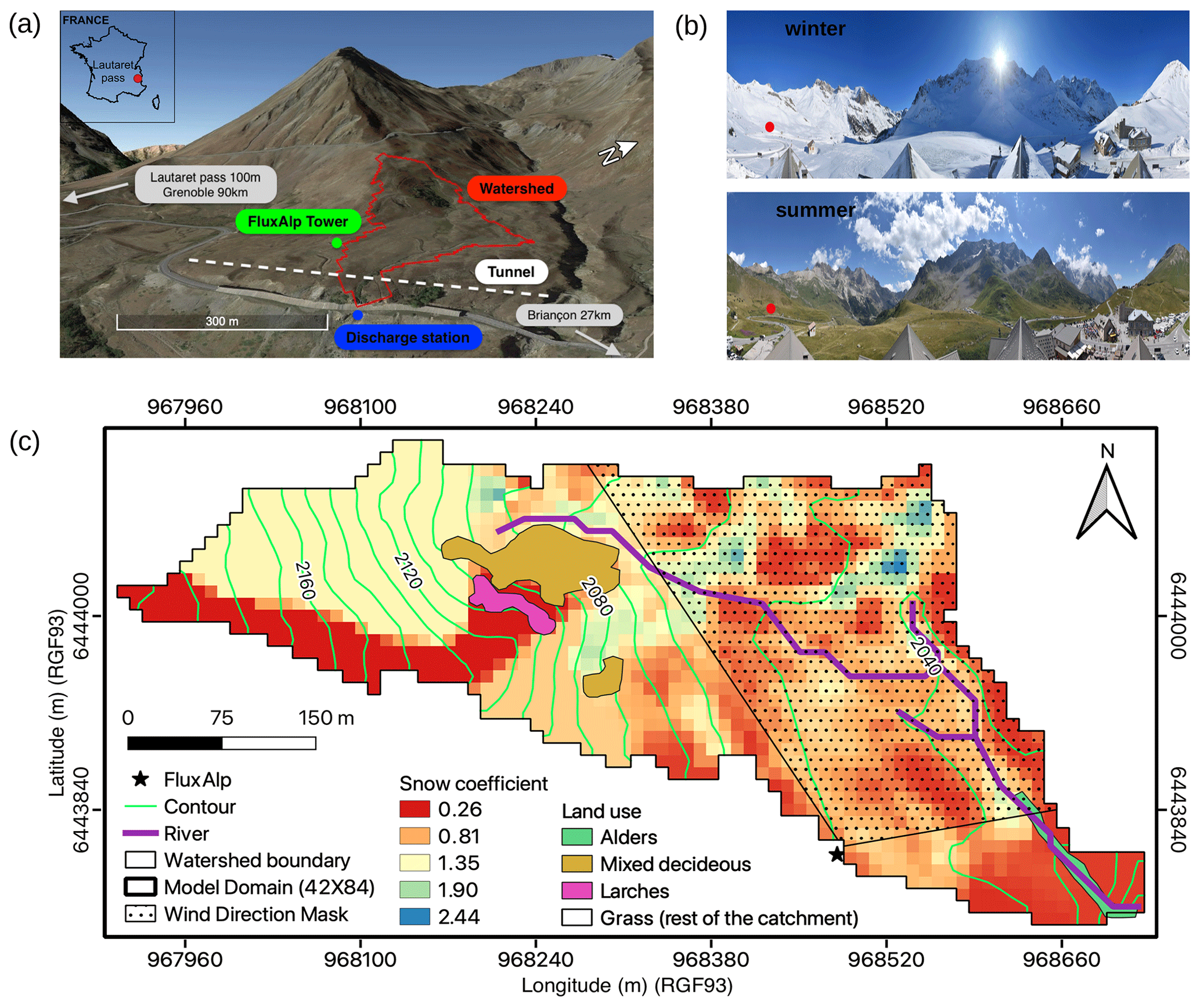
Figure 1 (a) Overview of the study area at Col du Lautaret, France; the small sub-alpine catchment is delineated in red, with the outlet at the blue point. The green dot (black star in (c)) is the FluxAlp micro-meteorological station. (b) Landscape views of the Lautaret pass area in winter (January) and summer (July). (c) Catchment domain (84×42 grid cells at 10 m resolution) with river branches (violet), elevation contours (green), and vegetation. Colored pixels represent the distributed snow coefficients. The dotted area is the approximated footprint for the daily wind directions considered for ET comparison in Sect. 3.3.

2.2 Climate

The study area is located in a typical mid-latitude alpine climate. Figure 2 shows meteorological observations for the simulated hydrological year from 11 November 2017 (the first snowy day) to 10 November 2018. The catchment has a long winter season, with 5 to 6 months of snowfall (Fig. 2a) and snow cover. The FluxAlp meteorological station records a total of 1530 mm yr⁻¹ precipitation, out of which 970 mm is snow in the studied period. According to 2017–2018 weather data, the site-average temperature is 4 ^∘C. The site temperatures show a strong seasonal contrast between below-zero winter conditions (−7.4 ^∘C minimum monthly mean in February) and a mild summer (14 ^∘C maximum monthly mean in July) (Fig. 2b). Winds higher than 5 ms⁻¹ (Fig. 2c) are common throughout the year, and are usually from the southwest direction along the mountain pass (Fig. 4a). Temperature and specific humidity follow the same cyclic pattern (Fig. 2d). March is the most humid period of the year, while July is the driest. Solar radiation (Fig. 2f) varies due to the seasonal cycle and to shading effects from the southern high mountain range (elevation 3000–4000 m elevation), which are particularly sensitive in the winter when the sun is lower on the horizon.

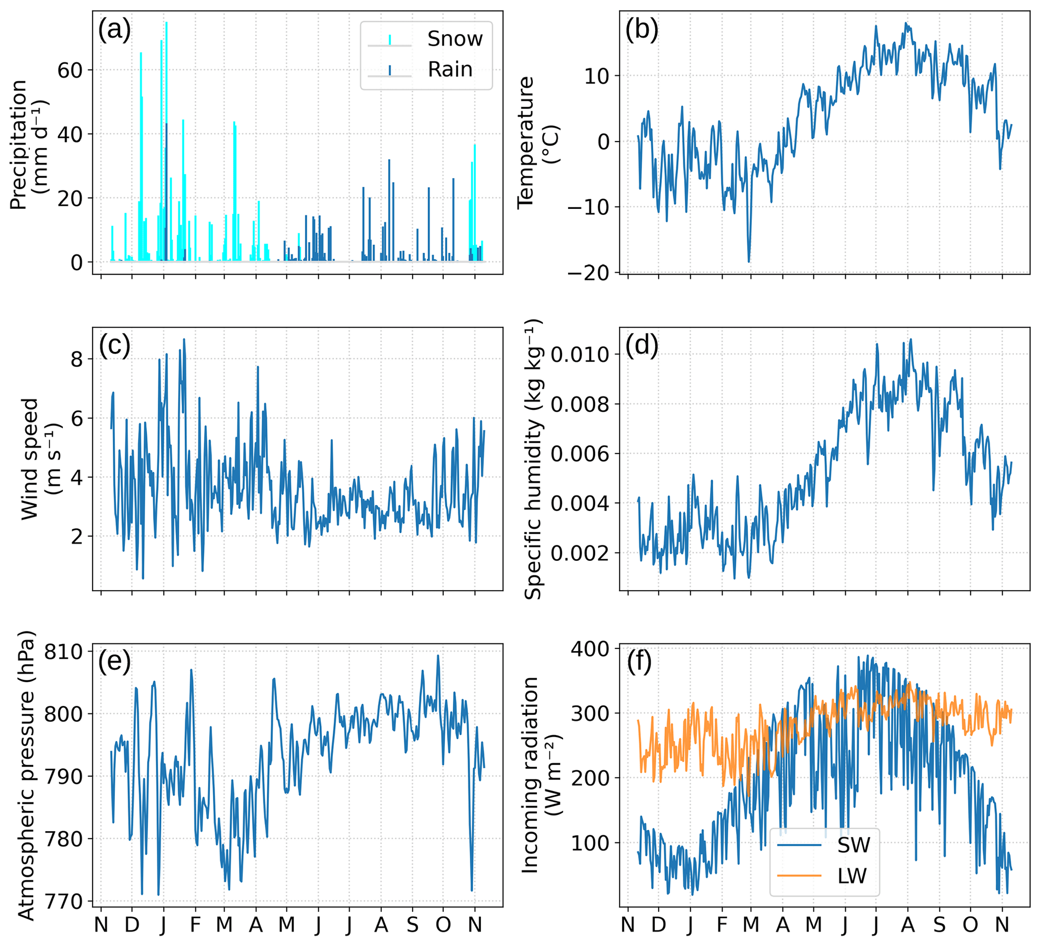
Figure 2 Daily meteorological observation at Col du Lautaret for the hydrological year 2017–2018: precipitation (a), air temperature (b), wind speed (c), specific humidity (d), atmospheric pressure (e), and shortwave (SW) and longwave (LW) incoming radiation (f).

2.3 Monitoring

Most of the monitoring on the site started in 2012. This includes the temperature and humidity (CS215, Campbell Scientific), atmospheric pressure (Setra CS100, Campbell Scientific), wind speed and wind direction (Vector A100LK anemometer and W200P, Campbell Scientific), four components of net radiation (CNR4, Kipp and Zonen), snow height (SR50A, Campbell Scientific), and NDVI (normalized difference vegetation index) measured using a Skye Instruments SKR1800. Since 2015, the site has received one eddy covariance station composed of a LI-COR LI-7200 close-path gas analyzer and a HS50 Gill 3D sonic anemometer. In 2017, an OTT Pluvio weighting rain gauge was installed at the FluxAlp weather station. Site setup, monitoring, and data processing follow the ICOS (https://www.icos-ri.eu/, last access: 18 November 2022) standards. All measured variables are recorded at 15 min time steps and then averaged over 30 min, except for precipitation, which is summed. The EddyPro software was used to process the turbulent fluxes at the same 30 min time steps following the ICOS recommendations (Hellström et al., 2016).

3 Methodology

3.1 ParFlow-CLM

In this study, we used ParFlow-CLM, an integrated surface–subsurface coupled hydrological model, to simulate the impact of distributed meteorological forcing on the water transfers (Jones and Woodward, 2001; Ashby and Falgout, 1996; Kollet and Maxwell, 2006, 2008; Maxwell, 2013; Maxwell and Miller, 2005). ParFlow is a parallel integrated hydrological model optimized to solve the surface and subsurface exchange of fluxes. ParFlow solves the three-dimensional Richards equation to calculate the water pressure field and transfer of fluxes between unsaturated and saturated porous media (Jefferson and Maxwell, 2015). Relative permeability and soil retention curves are based on the Van Genuchten relationships (Van Genuchten, 1980). A multigrid-preconditioned conjugate gradient solver and the Newton–Krylov solver for nonlinear equations (Kuffour et al., 2020) make the model efficient to run in a parallel computing environment. ParFlow includes a terrain-following grid which eases boundary condition prescription. It accounts for the surface slope in Darcy's formula, which also eases the numerical exchange between subsurface and overland flow. At the model surface, there is an excess of water (pressure>P_atm) in all saturated cell flows according to the two-dimensional kinematic wave equation (Kuffour et al., 2020). ParFlow then maintains a continuous pressure head value from the bottom to the top of the domain and explicitly calculates fluxes between groundwater and surface water. Infiltration excess (Horton, 1933) or saturation excess (Dunne, 1983) runoff is then generated according to the Richards equations. Flow routing uses the D4 scheme to determine the flow direction based on individual slopes in the x and y directions and has been calculated according to Condon and Maxwell (2019). The CLM (Common Land Model) is a land surface model designed to compute the land–water–energy exchange between the Earth's surface and atmosphere (Dai et al., 2003). CLM accounts for land cover, surface temperature, soil moisture, soil texture, soil color, root depth, leaf and stem area, roughness length, displacement height, plant physiology, and thermal and optical properties of the medium to calculate the surface energy and water balance. It calculates evapotranspiration as the sum of evaporation, vegetation evaporation, transpiration, and re-condensation. CLM models snow with up to five layers, following the layer thickness and temperature, water, and ice mass in each layer. The CLM two-stream radiative transfer scheme accounts for direct and scattered radiation by snow at visible and near-infrared wavelengths. In CLM, when pixels cover a large range of elevation, the snow fraction is used to calculate the total snow cover area. In our study, the snow fraction was assigned values of 0 (no-snow) or 1 (snow). Our horizontal pixel resolution is small enough (10×10 m) that we consider the snow cover in a pixel to be uniform. This implies that our pixels are either completely covered with or completely devoid of snow. Therefore, CLM can handle the spatial/temporal snow distribution, associated water fluxes (melting, sublimation, infiltration), and evaporative fluxes according to spatial/temporal heterogeneous surface conditions (temperature, water/snow inputs, incoming radiation, wind speed, and vegetation). After computing the surface exchanges, such as evaporation, transpiration, snowmelt, and precipitation infiltration into and out of the soil, these are applied as sources/sinks in the Richards equations. Further information on ParFlow terminology and the model's capability is included in the user manual (https://github.com/parflow, last access: 18 November 2022).

3.2 Meteorological distribution

3.2.1 Precipitation

The precipitation data from the rain gauge was first processed to account for the lack of a gauge shield (Klok et al., 2001). The adopted algorithm was

$$\begin{array}{}\text{(1)}& P_{\mathrm{corr}}(x_{\mathrm{0}},y_{\mathrm{0}})=P(x_{\mathrm{0}},y_{\mathrm{0}})\cdot (a+b\cdot u(x_{\mathrm{0}},y_{\mathrm{0}}\left)\right),\end{array}$$

where P_corr is the corrected precipitation (mm), P is the measured precipitation (mm) at the observation station, u is the wind speed at the observation station in m s⁻¹, and a and b are correction factors that are different for rain (a=1.04, b=0.04) and snow (a=1.18, b=0.20) (Sevruk and WMO, 1986).

To account for snow-cover spatial variability in the catchment domain, S_c(x,y), the precipitation that fell as snow at location (x,y) was calculated using a snow coefficient map, C_s(x,y). The snow coefficient map was prepared from the ratio between the measured snow height at the gauge and the snow height measured through a laser scan on the same day (21 February 2018) at the end of the accumulation period (Fig. 1). The snow height was calculated from the laser, and was the difference between the apparent snow height (from the laser scan) at the end of the accumulation period and the digital elevation model (DEM) for the surface without snow. The snow DEM and surface DEM were prepared at a resolution of 2 m and were upscaled to 10 m resolution using the minimum of each cell. The S_c(x,y) calculation hypothesizes that the distributed snow cover on that date aggregates all spatial heterogeneity of the snow deposition, including snow transport (redistribution). It also includes the snow compaction between the date of deposition and the laser scan. Then the corrected precipitation that had fallen as snow was calculated according to

$$\begin{array}{}\text{(2)}& S_{\mathrm{c}}(x,y)=S_{\mathrm{m}}(x_{\mathrm{0}},y_{\mathrm{0}})\cdot C_{\mathrm{s}}(x,y)),\end{array}$$

where S_m(x,y) is the measured snow precipitation at the observation station. It must be noted that the laser scan did not cover the upper part of the catchment. Zones not covered by the scanner were each given a fixed value according to our field observations. Moreover, due to the small size of the catchment and the low elevation range (1993 to 2204 m), precipitation gradients between upper and lower elevations have not been considered, and the rain has not been distributed in our study.

3.2.2 Shortwave radiation

The shortwave radiation, SW_c(x,y), was distributed from the observed shortwave radiation measurement, SW_m(x₀,y₀), at the meteorological station considering the sun's position and the terrain effect (Liston and Elder, 2006). Equation (3) partitions diffuse (30 %) and direct (70 %) shortwave radiation contributions from the observed shortwave radiation, and Eq. (4) accounts for the terrain features based on their orientation, which was integrated as a solar cosine function in Eq. (3). The partition of diffuse and direct shortwave radiation was taken from the CLM technical setup (Oleson et al., 2004).

$$\begin{array}{}\text{(3)}& {\displaystyle }{\mathrm{SW}}_{\mathrm{c}}(x,y)=\left(\mathrm{0.7}\cos i\right(x,y)+\mathrm{0.3})\cdot {\mathrm{SW}}_{\mathrm{m}}(x_{\mathrm{0}},y_{\mathrm{0}})),\text{(4)}& {\displaystyle }\begin{array}{rl}\cos i(x,y)& =\cos \mathit{\beta }(x,y)\cdot \cos Z(x,y)+\sin \mathit{\beta }(x,y)\\ & \cdot \sin Z(x,y)\cdot \cos \left(\mathit{\mu }\right(x,y)-{\mathit{\xi }}_s(x,y\left)\right).\end{array}\end{array}$$

Here, SW_c is the corrected shortwave radiation (W m⁻²) at a coordinate location, SW_m is the measured shortwave radiation at the observation station, and i is the solar angle function of the slope angle β, the slope southern azimuth ξ_s, sun southern azimuth μ, and solar zenith angle Z.

3.2.3 Wind speed

Wind speed was spatialized to better account for the estimation of turbulent fluxes (Liston and Elder, 2006). The wind speed was distributed as

$$\begin{array}{}\text{(5)}& {\displaystyle }{W}_{\mathrm{w}}(x,y)=\mathrm{1}+\mathrm{0.58}{\mathrm{\Omega }}_{\mathrm{s}}(x,y)+\mathrm{0.42}{\mathrm{\Omega }}_{\mathrm{c}}(x,y),\text{(6)}& {\displaystyle }{\mathrm{\Omega }}_{\mathrm{s}}(x,y)=\mathit{\beta }(x,y)\cdot \cos \left(\mathit{\theta }\right(x,y)-\mathit{\xi }(x,y\left)\right),\text{(7)}& {\displaystyle }\begin{array}{rl}{\mathrm{\Omega }}_{\mathrm{c}}(x,y)& =\mathrm{0.25}\sum \left(z\right(x,y)-\mathrm{0.5}(z_i(x,y)\\ & +z_j(x,y)\left)\right)/d,\end{array}\text{(8)}& {\displaystyle }{W}_{\mathrm{c}}(x,y)=W_{\mathrm{w}}(x,y)\cdot W_{\mathrm{m}}(x_{\mathrm{0}},y_{\mathrm{0}}),\end{array}$$

where W_w is the wind weighting factor at a coordinate location as a function of wind direction slope (Ω_s) and curvature (Ω_c), i and j are the search direction (N–S, E–W, NE–SW, SE–NW), d is 2η for cardinal axes and $\mathrm{2}\sqrt{\mathrm{2}}\mathit{\eta }$ for others, η is the search distance, z is the elevation, β is the slope angle, θ is the wind direction, and ξ is the slope azimuth. The search distance d for curvature was set to 50 m (Revuelto et al., 2020). Finally, the wind weighting factor (W_w) was multiplied by the wind speed measured at the observation station (W_m, m s⁻¹) to obtain the terrain-corrected wind speed (W_c).

Along with precipitation, shortwave radiation, and wind speed, three more variables are used to force the model: temperature, pressure, and specific humidity. However, as the model was set to a microscale catchment with little elevation variability, we did not distribute these parameters.

3.3 Wind direction mask

To compare the simulated evapotranspiration (ET) with the observation, a wind direction mask was prepared to approximately represent the eddy-covariance station footprint area. As the catchment and the footprint area only partly coincide, we selected simulated pixels in an approximated footprint area based on a wind direction mask (Fig. 1) and averaged simulated values over the mask. The wind direction mask was prepared according to the prevailing wind directions towards the Flux’Alp station between the 10th percentile (122.39^∘) and 90th percentile (260.51^∘) wind directions. We then compared the observed evapotranspiration to the simulated average value over the mask only when the wind blows from a direction included in the mask, as this maximizes the comparability of simulated and measured values.

3.4 Sentinel-2 snow cover

Snowmelt dynamics were compared to Sentinel-2A and Sentinel-2B products from the Sentinel-2 mission developed by the European Space Agency (ESA) for high-resolution satellite imagery (Drusch et al., 2012). We downloaded four Sentinel-2 images, out of which two belong to the accumulation period and two to the melting period. These images were selected to show the spatial and temporal distribution of snow in the catchment. For this purpose, we have calculated the normalized snow difference index (NDSI) from the downloaded images as (Dozier, 1989)

$$\begin{array}{}\text{(9)}& \mathrm{NDSI}={\displaystyle \frac{\mathrm{Green}\left(\mathrm{band}\mathrm{3}\right)-\mathrm{SWIR}\left(\mathrm{band}\mathrm{11}\right)}{\mathrm{Green}\left(\mathrm{band}\mathrm{3}\right)+\mathrm{SWIR}\left(\mathrm{band}\mathrm{11}\right)}},\end{array}$$

where “Green” and “SWIR” are the corresponding bands in the green and shortwave infrared regions of the satellite, respectively. The green band is represented by “band 3” and the SWIR band is represented by “band 11” in the Sentinel-2 product. Sentinel band 3 was available at 10 m resolution while band 11 was at 20 m resolution. The NDSI calculation was carried out by resampling band 11 at 10 m resolution (Hofmeister et al., 2022). The Sentinel-2 snow pixels were selected with NDSI > 0.4 (Riggs et al., 1994). In the model, the snow pixels were selected as those with a snow depth of over 1 cm, which is the minimum non-zero height for snow.

3.5 Performance indicators

3.5.1 Slope

The slope for linear regression without an intercept (y=αx) is represented as

$$\begin{array}{}\text{(10)}& \mathit{\alpha }={\displaystyle \frac{{\sum }_{i=\mathrm{1}}^n\left(x_i{y}_i\right)}{{\sum }_{i=\mathrm{1}}^n\left(x_i^{\mathrm{2}}\right)}},\end{array}$$

where x is the observed value and y is the predicted value. The slope was calculated for evapotranspiration using hourly values.

3.5.2 R-square (R²)

The R-square or coefficient of determination is defined as

$$\begin{array}{}\text{(11)}& {\left[{\displaystyle \frac{{\sum }_{i=\mathrm{1}}^n(x_i-\stackrel{\mathrm{‾}}{x})(y_i-\stackrel{\mathrm{‾}}{y})}{\sqrt{{\sum }_{i=\mathrm{1}}^n(x_i-\stackrel{\mathrm{‾}}{x}{)}^{\mathrm{2}}}\sqrt{{\sum }_{i=\mathrm{1}}^n(y_i-\stackrel{\mathrm{‾}}{y}{)}^{\mathrm{2}}}}}\right]}^{\mathrm{2}},\end{array}$$

where x is the observed value, y is the predicted value, and $\stackrel{\mathrm{‾}}{x}$ and $\stackrel{\mathrm{‾}}{y}$ are the means of the observed and predicted values, respectively. The R² was calculated using hourly values for evapotranspiration and daily mean values between 10:00 to 14:00 h for albedo.

3.6 Root mean square error (RMSE)

The RMSE score is represented as

$$\begin{array}{}\text{(12)}& \sqrt{{\displaystyle \frac{\mathrm{1}}{n}}\sum _{i=\mathrm{1}}^n(x_i-y_i{)}^{\mathrm{2}}},\end{array}$$

where n is the number of samples and x is the observed value, while y is the predicted value. The RMSE was calculated using hourly values for evapotranspiration and daily mean values between 10:00 to 14:00 h for albedo.

3.7 Mean bias error (MBE)

The MBE score is represented as

$$\begin{array}{}\text{(13)}& \sqrt{{\displaystyle \frac{\mathrm{1}}{n}}\sum _{i=\mathrm{1}}^n(y_i-x_i)},\end{array}$$

where n is the number of samples and y is the predicted value, while x is the observed value. The MBE score is represented for the Sentinel-2 images as an average between the spatial similarity of snow and non-snow pixels (mismatch between the image pixels).

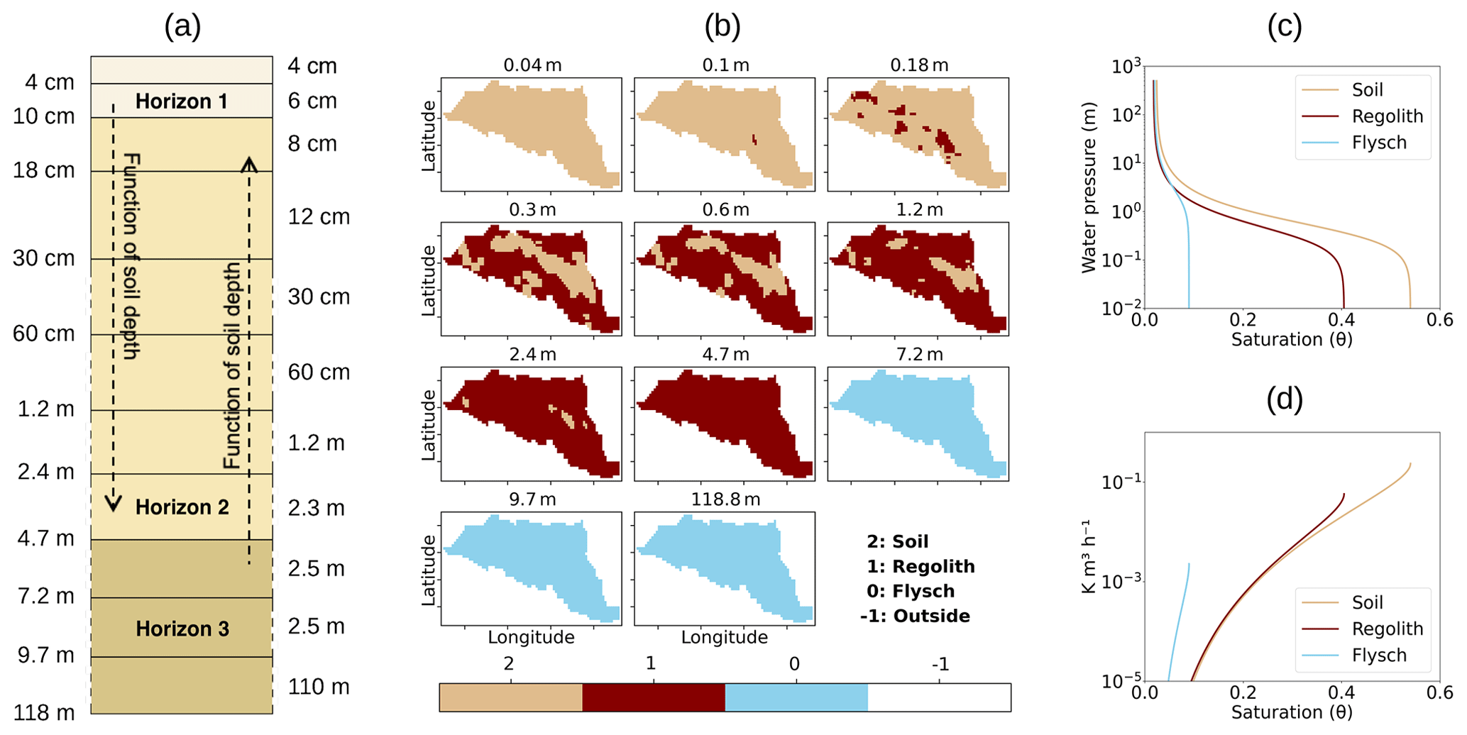
Figure 3 Subsurface configuration used for discretizing the domain. (a) The vertical distribution of the subsurface layer with the thickness (right) and depth (left) of each grid cell. (b) Spatial distribution of the subsurface horizons, including soil (burly wood), regolith (dark brown), and flysch (blue). These horizons vary in their hydro-geological parameters (e.g., in terms of conductivity and porosity) according to the soil transfer functions shown in the soil retention curve (c) and the hydraulic conductivity curve (d).

4 Domain discretization and simulation setup

The surface domain of 15.28 ha was discretized at a horizontal hyper-resolution of 10 m with a total number of $\mathrm{84}\times \mathrm{42}\times \mathrm{11}$ (longitude × latitude × levels) cells on a terrain-following grid (Fig. 1). Individual cell height (z-direction levels) varied from 4 cm for the top soil layer to 110 m for the deepest layer (Fig. 3a). The model was mainly built and forced using the observations; hence, the input data belongs to either observation data or data derived from observation. These data include temperature, precipitation, wind speed, shortwave radiation, humidity, and atmospheric pressure, as plotted in Fig. 2. Leaf area index (LAI) was calculated from NDVI measurements, while stem area index (SAI) was assigned a constant value based on the field survey. Displacement height (d) and roughness length (z0) were calculated from the vegetation height following Brutsaert's rules (Brutsaert, 1982). The snow height sensor showed sensitivity to the grass height when there was no more snow on the ground. We, therefore, used the signal from this sensor when NDVI values were above 0.4 to estimate grass height. A lidar digital surface model (DSM) of 2 m resolution was available for the catchment and upscaled to 10 m resolution using the minimum of each cell. The upscaled DSM was processed with PriorityFLOW to generate the slope maps in the x and y directions (Condon and Maxwell, 2019). The land cover map was made through field observations, while the Manning coefficients were assigned using the land cover map. River pixels were assigned a constant Manning value of 0.05 s m${}^{-\mathrm{1}/\mathrm{3}}$, and the rest of the catchment was assigned a constant Manning value of 0.03 s m${}^{-\mathrm{1}/\mathrm{3}}$. The lateral and bottom boundary conditions were set to no flow, and the surface boundary condition was set at atmospheric pressure, which allowed fluxes to leave at a positive hydraulic head (Kollet and Maxwell, 2006). Hence, the inflow and outflow were restricted to exchange only through the surface. The subsurface was made heterogeneous with three soil horizons consisting of soil, regolith, and flysch with 11 different layers (Fig. 3a). The bottom of the domain was set deep enough to accommodate various subsurface water transfers (118 m deep from the surface). The soil physical parameters used in this study include porosity, permeability, soil horizons, and Van Genuchten parameters. The resulting water retention curves are plotted in Fig. 3c, d for the three different horizons. They show a reduction of permeability and porosity with depth. The soil horizon distribution (Fig. 3b) was determined from an electromagnetic survey measuring apparent electrical conductivity (related to water and clay content) and a ground-penetrating radar (GPR) measuring soil thickness. The electromagnetic survey was done for the whole catchment; however, the GPR survey was performed for three transverse profiles across the stream to validate the electromagnetic survey. Field permeability experiments and laboratory mercury porosity experiments determined the soil properties. Elaboration about the detailed hydro-geological characterization is beyond the scope of this study and will be detailed in a companion paper (Gupta et al., 2022). This study is more focused on surface dynamics due to meteorological variable distribution.

The model was forced with half-hourly meteorological forcing; however, the results were saved at hourly time steps. The Universal Time zone (UTC) was considered in terms of monitoring and modeling for this study. Before running the actual simulations, a 10-year spin-up run was performed with “SeepageFace” (no runoff) conditions to bring the model into hydrological balance. The yearly subsurface storage difference was used to evaluate whether the spin-up had taken the model into equilibrium, which happened at the end of the 10th year. Each simulation was also run for 2 consecutive years with the same forcing to avoid any imbalance in subsurface storage (Ajami et al., 2014). The different simulation setups for this study are detailed in Table 1.

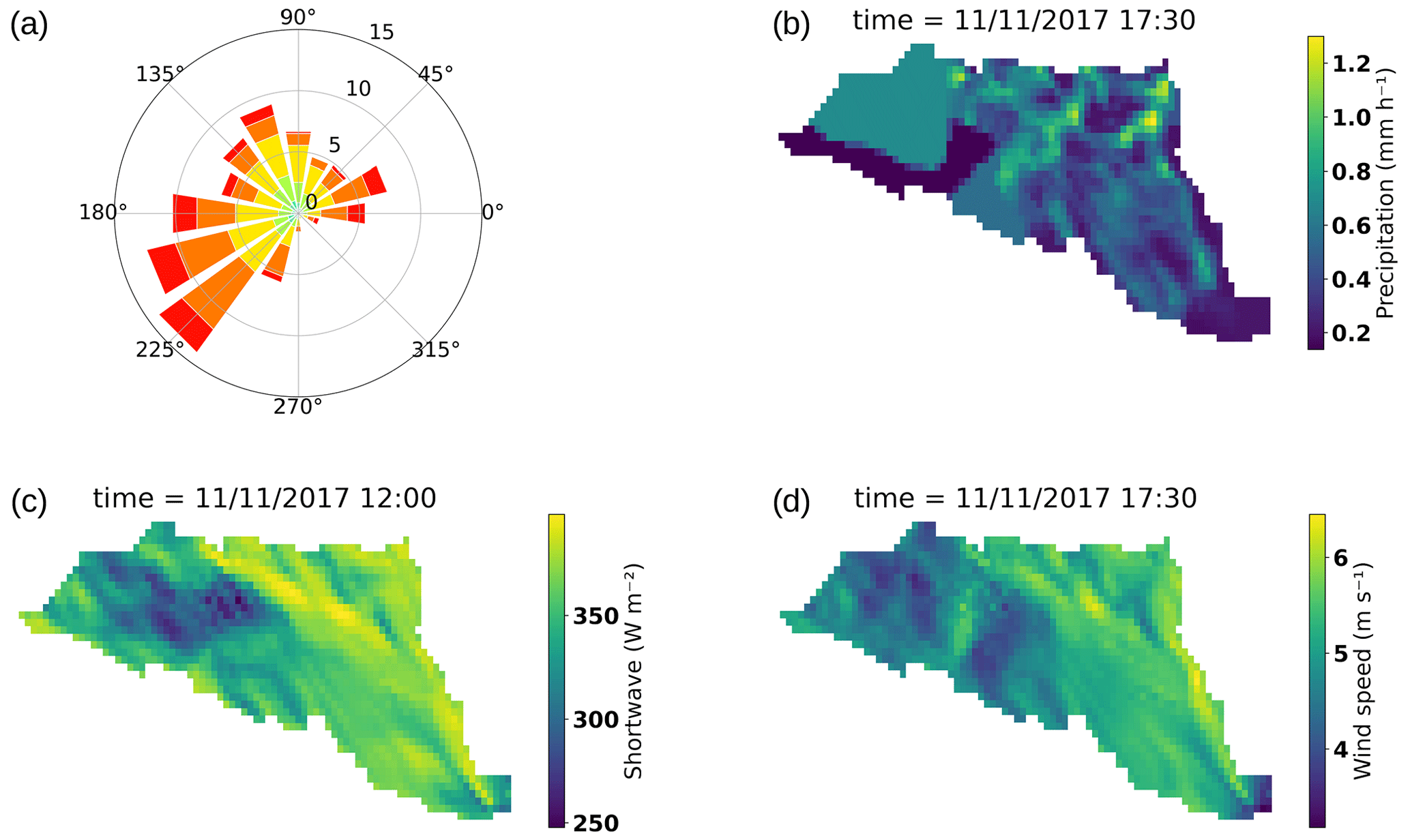
Figure 4 (a) Wind rose diagram. (b) Precipitation distribution along the catchment. (c) Shortwave radiation distribution over the catchment. (d) Wind speed distribution over the catchment. All are plotted for 11 November 2017 at 05:30 pm and 12:00 pm for shortwave radiation.

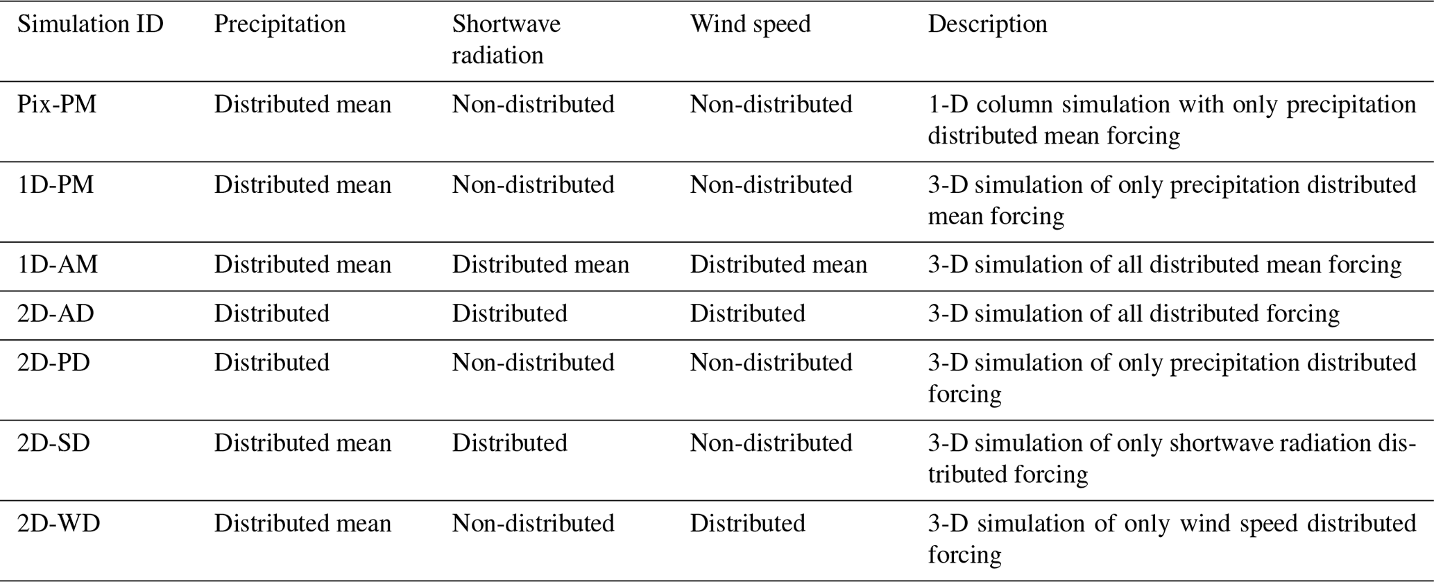
All simulations named “1D” use forcings that are uniform across the watershed (Table 1). Rain is the significant hydrological model input; hence we keep the same amount of precipitation input in all simulations (1443.72 mm), which corresponds to the spatial average of precipitation after applying the distribution correction (Eq. 2). Precipitation is reduced compared to what is measured at the rain gauge station (1531.96 mm) because the precipitation distribution process leads to a non-conservative spatial snow distribution over the catchment. The equal amounts of precipitation input lead us to easily see the partitioning between different hydrological fluxes across the different meteorological forcing simulations. 1D-PM, therefore, corresponds to a classical hydrological simulation for a small catchment when one applies the meteorological forcing directly from a nearby weather station. By contrast, 1D-AM accounts for local terrain slope and aspect according to Eqs. (5)–(8), and applies the mean corrected incoming radiation uniformly across the watershed. Therefore, the shortwave radiation amount is not the same when considering the measured value (yearly averaged shortwave radiation, 1D-AM: 190.8 W m⁻²) and the mean distributed value (yearly averaged shortwave radiation, 1D-PM: 152.1 W m⁻²): as the weather station is less shaded than the generally east-facing watershed, accounting for slope and aspect reduces the average incoming radiation. Meteorological parameters were further distributed to better analyze their respective influences. Pix-PM, 2D-PD, and 2D-WD all relate to 1D-PM and used the zenithal solar radiation observation (measured shortwave radiation) directly from the radiation sensor 2D-AD, and 2D-SD is related to 1D-AM as they used the same distributed incoming solar radiation according to Eqs. (5)–(8). The latter four proposed simulations were run to quantify the effects of all spatially distributed forcings together or individually (Table 1).

Meteorological forcings were distributed according to algorithms described in Sect. 3.2 to represent the effects of slope, curvature, and aspect on the spatial distribution of those forcings. Figure 4 presents snapshots of heterogeneities produced by these algorithms. Even at a micro-scale, one can observe the spatial meteorological variability along the grid after applying Eqs. (2)–(8). In Fig. 4b, for an averaged 0.53 mm snow rate, the distribution algorithm produces large heterogeneities ranging from 0.2 to 1.2 mm, with deeper accumulation occurring mainly on lowlands. Similarly, for shortwave radiation (Fig. 4c), for input radiation of 400.8 W m⁻² on 11 November at noon, the algorithm reduced the radiation to 349.7 W m⁻² on average, with a difference of more than ± 50 W m⁻² depending on the location. In wind speed distribution, there was not so much variation in the spatial mean before and after wind speed distribution. The mean wind speeds before and after spatial distribution were 5.6 and 5 m s⁻¹, respectively (Fig. 4d).

Table 1 Distributed and non-distributed approach adopted for different simulations.

5 Results

5.1 Simulations with spatially uniform forcings

1D-PM and 1D-AM represent our reference simulations, with uniform forcings across the watershed (see Table 1). Their results are presented in Fig. 5. According to the 1D-PM simulation (Fig. 5a), the hydrological year begins with the snow accumulation period until the end of March. December and January were the snowiest periods, with some snowmelt events (magenta line) due to short above-zero-degrees episodes which generate very little runoff (black line). In April, warmer positive temperatures and rain on snow events generate continuous melting in our simulation and produce the highest river discharge peaks with a strong daily cycle that are further intensified by coinciding rain events. This period also increased the subsurface storage, which produces a base flow later in May (Fig. 5b). In May, the streamflow shows a combination of base flow and snowmelt (snowmelt in May in Fig. 5a; subsurface storage decrease in May in Fig. 5b).

Figure 5 (a) Precipitation (rain in blue and snow in light blue), streamflow (black), snowmelt (magenta), and net radiation (green) regimes along the simulation period for the only precipitation distributed mean simulation (1D-PM). (b) Monthly water budget for the 1D-PM simulation, including rain (blue), snow (light blue), runoff (red), ET (green), and condensation (purple). The dotted black line is the total subsurface water storage. Panels (c, d) are the same as (a) and (b) but for the all distributed mean simulation (1D-AM). VD is the volume difference between plotted simulations as a percentage.

One of the most important and noticeable points while using non-distributed forcing was the sudden disappearance of the snow at the end of the snowmelt season, which usually not observed in the field. This means that all the pixels behaved in the same way, and there was no noticeable impact on the catchment spatial snow variability when considering a uniform forcing. From June to the beginning of the next snow period, summer rain produced an almost instantaneous river response and subsurface storage sustained the stream runoff for several months. During this period, one can note a radical change in net radiation because of the land cover change from snow to grass. The net radiation contributes to the snowmelt in early spring. The factors responsible for this phenomenon include the higher sun elevation, clear sky conditions, and higher daily temperature.

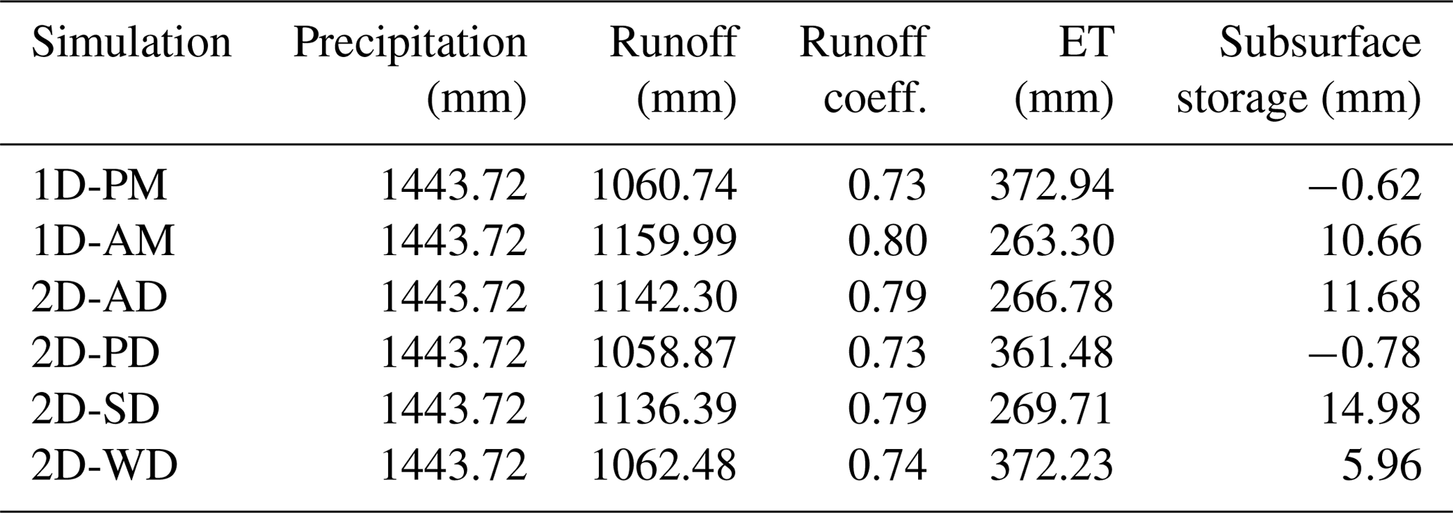
Table 2 Annual water budget terms in the catchment for different simulations.

During winter and spring, the monthly cumulated ET was very small (Fig. 5b) because of the low available energy and complete snow cover. After the complete snowmelt, the model simulated much higher monthly cumulated ET, in accord with the LAI cycle. During this period, ET was higher than the monthly cumulated rain (June, July, September), which means that ET participates in the extraction of shallow water storage during the summer. This can be seen by the difference in subsurface storage decline between the summer (higher water storage diminution) and the winter (lower water storage diminution). In October, one can notice a small increase in the subsurface storage when ET decreases because of vegetation decay. At the end of the hydrological year, the subsurface water storage has a deficit of −0.62 mm, which is much smaller than the annual cycle amplitude.

The 1D-AM simulation (Fig. 5c, d) mostly differs from 1D-PM as precipitation, solar radiation, and wind velocity were prescribed using the spatial average of the distributed forcing. This reduces the solar radiation from 190.8 to 152.1 W m⁻² on average, which reduces melting and ET. Snow lasts 9 more days on the ground, runoff increases from 73 % to 80 % of total precipitation (runoff coefficient, Table 2), and infiltration increases by 10.66 mm. For a similar geomorphology, any reduction in input solar radiation because of the catchment orientation or something else leads to higher water tables and then a higher runoff coefficient. Compared to the 1D-PM simulation, this simulation showed reduced runoff peaks in the early melt season, which leads to more percolation. Increased percolation leads to a higher base flow during the late summer and delays the base flow response by around 1 month compared to 1D-PM simulation. Runoff in the 1D-AM simulation increases overall by 9.4 % compared to the 1D-PM simulation.

5.2 Simulations with spatially distributed forcing

This section presents the simulation run with a fully distributed forcing (2D-AD), its difference from the previous uniformly forced simulations, and the three simulations based on forcings with only one distributed variable (2D-WD, 2D-PD, 2D-SD) to explore the contributions of each individual spatial distribution. Figure 6a shows that snowmelt lasts longer in the 2D-AD simulation, tailing across June and early July, with streamflow decreasing until even later in July. These snowmelt dynamics were smoother than were simulated in either uniformly forced simulation (1D-PM and 1D-AM), and correspondingly impact the net radiation, recharge, and streamflow discharge dynamic. In the most intense melt period in May, this resulted in ∼30 % lower peak streamflow values in 2D-AD compared to 1D-AM or 1D-PM simulations. However, the resulting annual water budget changed by only 2 % between 1D-AM and 2D-AD simulations, and by −7 % between 1D-PM and 2D-AD simulations. As mentioned in the previous section, the time-averaged distributed shortwave radiation input was lower in simulation 1D-AM compared to 1D-PM, as it accounted for shading effects. Simulation 2D-AD has the same time-average radiation input as 1D-AM and was closer to this simulation in the yearly budget. The small-scale distribution of meteorological forcings therefore only adds information on dynamics, not on yearly budgets. The tailing snowmelt through June generated more percolation to the subsurface, resulting in stronger base flow in late summer, thereby catching up with the total runoff volume simulated in 1D-AM.

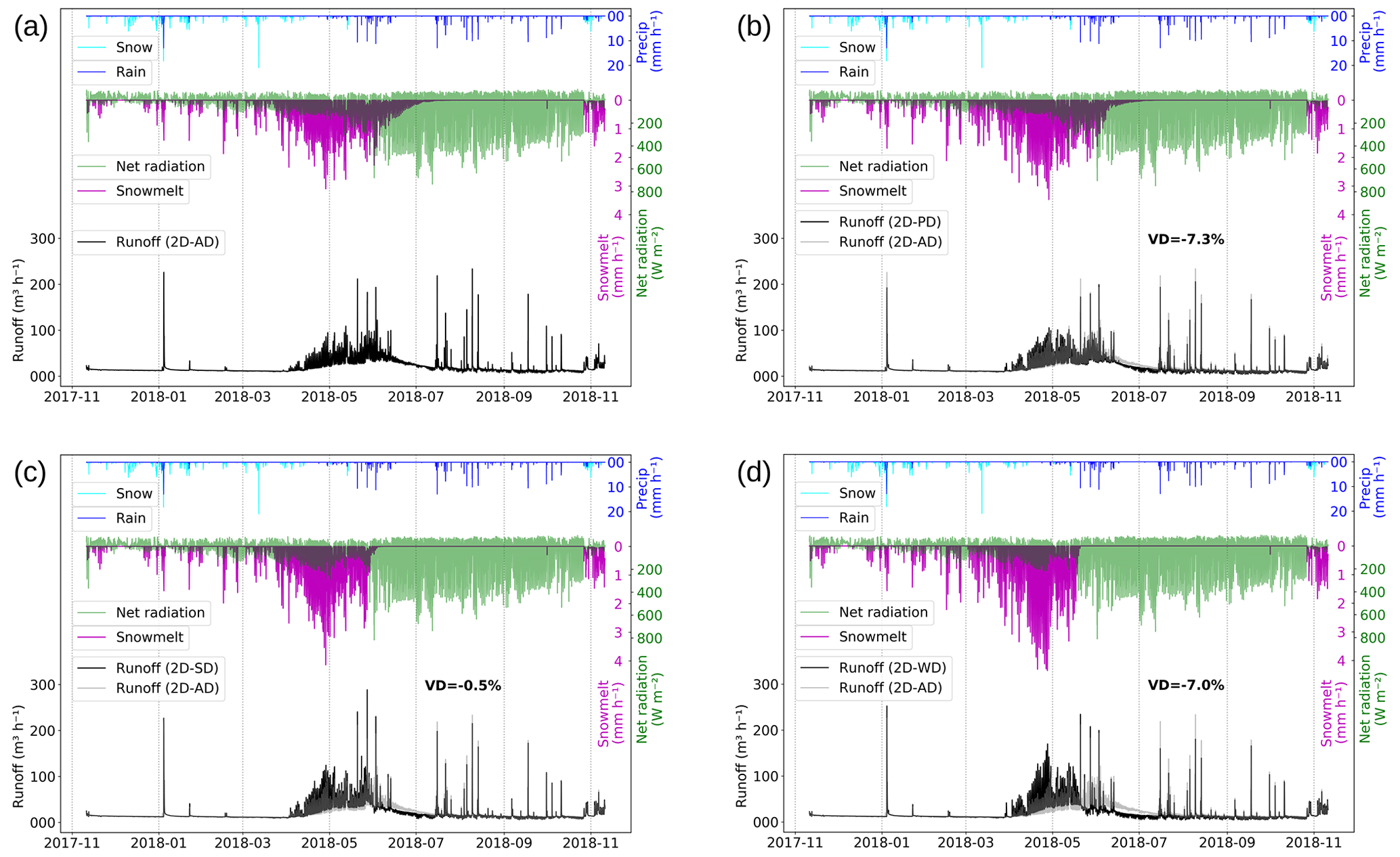
Figure 6 Same as Fig. 5a for (a) the all distributed run (2D-AD), (b) the only precipitation distributed run (2D-PD), (c) the only shortwave radiation distributed run (2D-SD), and (d) the only wind speed distributed run (2D-WD). VD is the volume difference between plotted simulations as a percentage.

As is visible in the results of the simulations with only one distributed forcing (Fig. 6b, c, d), the smoother decline in snowmelt resulted from both precipitation and shortwave radiation distribution. However, the simulation 2D-WD, where only the wind speed forcing was distributed, did not present such a smooth decline in snowmelt, and results were very similar to the non-distributed simulation (1D-PM). The melting period tail length was controlled by the snowpack depth variability (Fig. 9a, b) and higher accumulated snow on some pixels. This combined with solar radiation effects, which also produced spatial variability in snowmelt on the catchment, even if the snow precipitation was uniformly distributed (Fig. 6c). The only wind speed distribution (2D-WD) simulation showed the highest melting regimes from mid-March to mid-May, when temperature and incoming radiation were favorable for melting, resulting in daily melting peaks larger than 4 mm h⁻¹ (Fig. 6d). In detail, wind speed distribution shows an increase in the melting rate, which leads to higher subsurface storage when compared to 1D-PM.

Streamflow differences between simulations basically follow the melting differences. The impact of the late April and early May rain-on-snow period on streamflow is visible in Fig. 6a, b. It must be noted that the incoming solar radiation differs between simulations. Due to the non-distributed shortwave radiation in 2D-PD simulation, the melting peaks were higher compared to 2D-AD simulation. This resulted in rapid runoff in 2D-PD simulation and less percolation to the subsurface, which caused a volume difference of −7.3 % compared to 2D-AD simulation. The 2D-WD and 2D-PD simulations showed lower streamflow values compared to 2D-AD and 2D-SD simulations. This happened because, for the former two, the catchment receives 38.7 W m⁻² less radiation than for the latter two. The shortwave radiation distribution slowed the melting, which enhanced percolation to the subsurface. This subsurface percolation appeared as the base flow in the late summer. Though the base flow in 2D-SD simulation was lower than in 2D-AD, due to equal precipitation in all pixels, the 2D-SD simulation showed higher early melting peaks (Fig. 6c). This counterbalance between 2D-AD and 2D-SD simulation showed a volume difference of only −0.5 %. In 2D-WD simulation, due to rapid runoff during the melting season, the subsurface storage decreased, which resulted in a far lower base flow with a volume difference of −7.0 % compared to 2D-AD simulation (Fig. 6d). To conclude, the amount of precipitation in a pixel correlated with the snowmelt peaks; however, rapid melting decreases the subsurface storage, which results in lowered streamflow. In the late summer period when the snow gets melted, these differences were not visible in the streamflow.

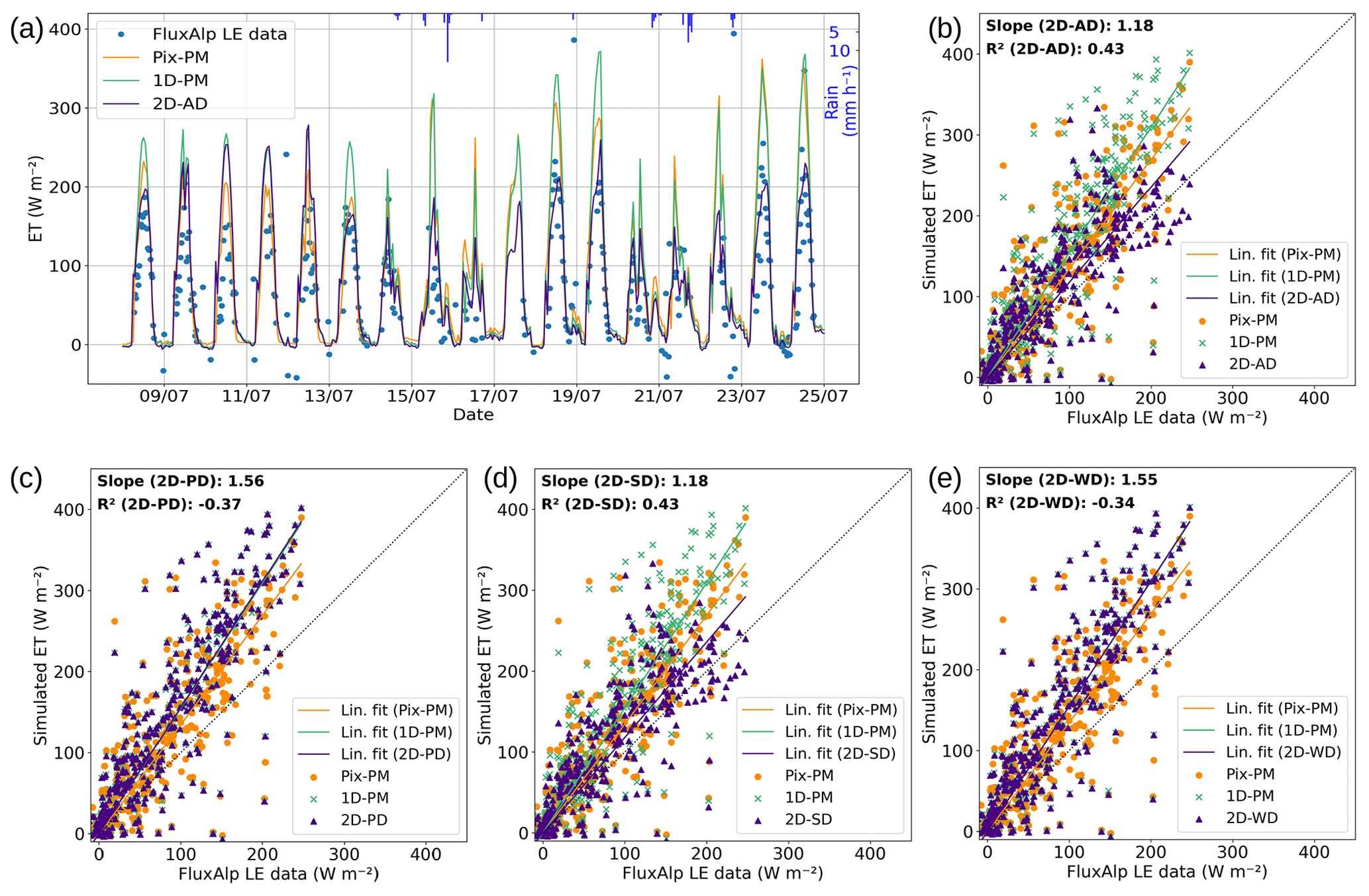
Figure 7 (a) Evapotranspiration simulation masked with a wind direction mask for 17 d in summer for the all distributed run (2D-AD). Scatter plot for the July to August 2018 period for (b) the all distributed run (2D-AD), (c) the only precipitation distributed run (2D-PD), (d) the only shortwave radiation distributed run (2D-SD), and (e) the only wind speed distributed run (2D-WD). Each slope line represents the corresponding linear fit to the scatter plot; the slope value of each simulation is highlighted at the top.

Evapotranspiration in the pixel run (orange curve and orange dots) was clearly overestimated compared to observed evapotranspiration, as one can see in both the time series and the scatter plots. Similarly, the non-distributed simulation (green curve and green dots, 1D-PM) and the distributed simulations 2D-PD and 2D-WD have comparable evapotranspiration amplitudes (Fig. 7c, e). However, 2D-AD and 2D-SD show reduced simulated ET, which better matches the observations (Fig. 7b, d). This reflects the lower (average) shortwave radiation in the forcings where the solar radiation was distributed according to the terrain (Sect. 4): as the catchment generally faces east, this distribution reduced the direct incoming solar radiation from noon to sunset.

The evapotranspiration in both Pix-PM and 1D-PM was overestimated compared to observations. First, the pixel run (Pix-PM) was supposed to simulate a catchment border (FluxAlp location) with drier soil/ground conditions (top of a ridge), and the ET observations were supposed to average both the wet zones close to the river and the drier zones. However, this was not the case in our 2D-AD and 2D-SD simulations. The linear slopes in these two simulations moved much closer to the identity line (slope = 1.18) compared to other simulations. This shows that, along with subsurface percolation, shortwave radiation distribution better simulated the ET. In 2D-PD and 2D-WD simulations, the linear slope equals the slope of the pixel run (slope = 1.55), which corresponds to much higher evapotranspiration compared to observations. Shortwave radiation distribution (Fig. 7d) showed the most important impact in our measurement area. Shortwave radiation distribution showed a smoothed runoff curve, higher subsurface percolation, increased base flow, and increased runoff. The corresponding reduced ET in 2D-SD (and 2D-AD), averaged for the footprint area, also corresponds much better to the observations.

5.3 Hydrological budget

Annual water budgets (Table 2) show that shortwave radiation distribution and the subsequent ET calculation have a large impact, making a difference of ∼100 mm at the annual budget scale. This increases runoff from 73 % to 79 % of the total annual precipitation by diverting the difference in flux towards runoff. This also results in a change in water storage over the year, as explained in the previous section. As we started from the same initial conditions for all simulations and additionally ran the spin-up for another 2 years, it reached more than 10 mm in subsurface storage when SW was reduced (1D-AM, 2D-AD, and 2D-SD), and 5.96 mm for 2D-WD simulation. The subsurface storage change remains much smaller than the ET difference and does not impact the runoff coefficient.

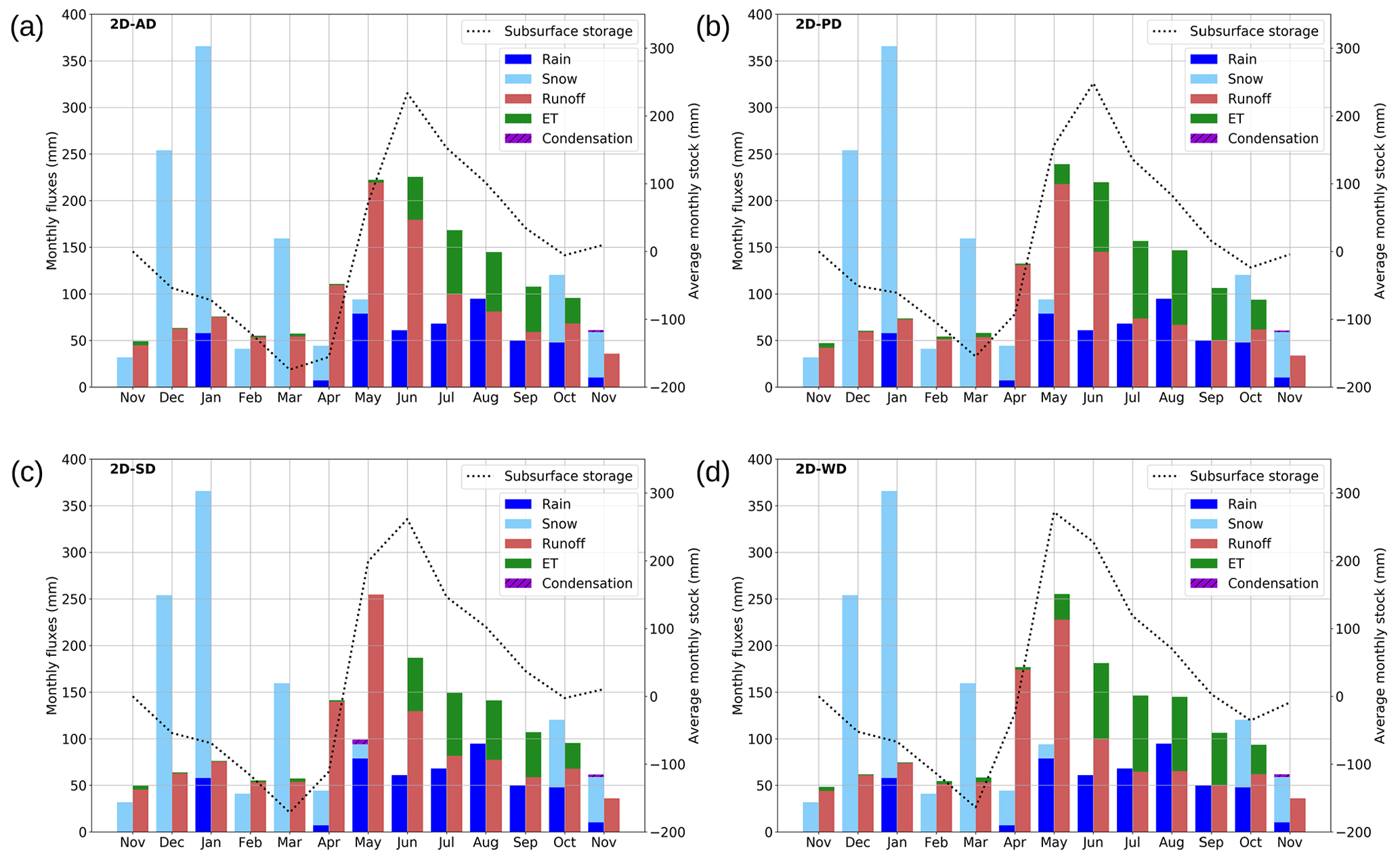
Figure 8 shows monthly water budgets for 2D-AD and individually distributed simulations. Snow precipitation from November to March does not infiltrate much to fill up the subsurface storage (dotted line). January rain-on-snow events slightly reduce the subsurface storage. Very similar runoff values were observed up to the end of February among the different scenarios. In contrast, from mid-March to June, the subsurface storage was replenished by melting (Fig. 6), which later increased the runoff. 2D-WD forcing produced the largest values of recharge (∼430 mm), and 2D-AD produced the largest values of streamflow. From May to October, the streamflow at the outlet and the ET decreased the subsurface storage. Higher shortwave radiation (2D-PD and 2D-WD) led to longer ET periods. Finally, one can note a reduction in ET because of vegetation senescence in November and the beginning of subsurface storage.

Figure 8 Same as Fig. 5b for (a) the all distributed run (2D-AD), (b) the only precipitation distributed run (2D-PD), (c) the only shortwave radiation distributed run (2D-SD), and (d) the only wind speed distributed run (2D-WD).

5.4 Snow dynamics

Figure 9 shows the temporal dynamics of the snow and the impact on albedo. Snow depth plots for the Pix-PM run (purple line) and the 1D-PM run (red line) were superimposed. The 1D-PM run shows little variability in snow depth (red shading). The dynamics of these two runs were consistent with the observations (black line), although snow height is overestimated during the initial accumulation period. This was probably because of the rough snow/rain partition temperature threshold and the inability of the snow scheme to account for compaction. The snowmelt dynamic was particularly well simulated (snow cover within the Sentinel-2 image acquisition date), especially during the dry period at the end of April. In early May, one can note some discrepancies again, probably because of our limited ability to separate rain and snow close to the phase-change temperature in the precipitation forcing. This can be seen in the simulated pixel albedo, which returned to its maximum snow albedo value at the end of the melting season (0.8), which was not the case in the observations. The simulated albedo mostly follows the observations; however, the snow age parameterization in the model was not adequate enough to simulate the albedo where observations showed that the albedo decreased during the melting period.

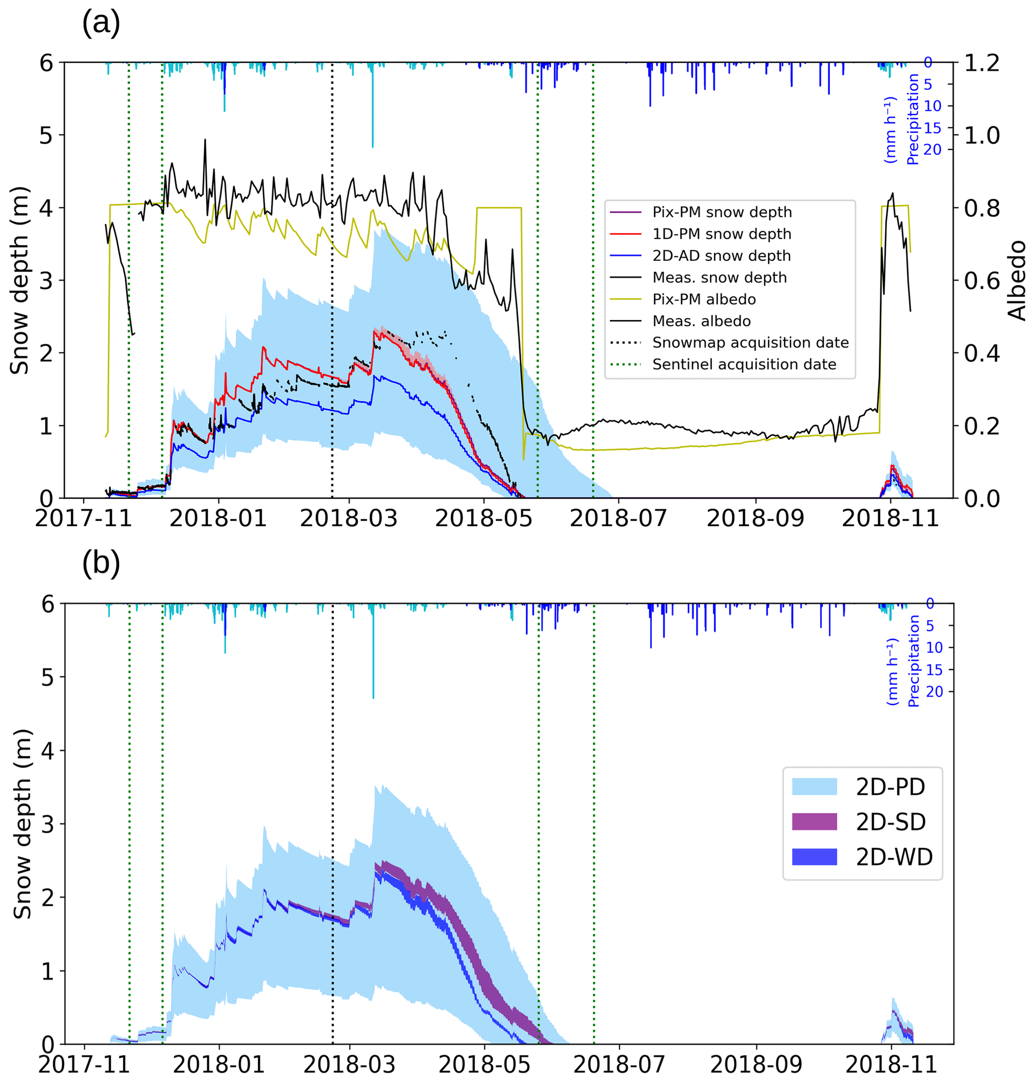
Figure 9 (a) Snow depths (left axis) for different simulations compared with observations (black line). Colored lines show the average depths over the catchment, and shading shows the spatial variability. Right axis: observed (black line) and 1D-PM-simulated (yellow line) albedo. Averaged precipitation (rain in blue and snow in cyan) is plotted at the top of the graph. Panel (b) shows the same as (a) but for the only precipitation (2D-PD), only shortwave radiation (2D-SD), and only wind speed (2D-WD) distributed runs.

In the 2D-AD simulation, the snow cover becomes discontinuous early in May, and some pixels stay covered with snow more than 1 month later compared to the 1D-PM simulation (Fig. 9a). Snow depth variability in the watershed, as indicated by the height of the shading in Fig. 9a, increases during the snow accumulation period and then diminishes during the snowmelt. This effect can also be seen in the 2D-PD simulation but not in any other distributed forcing simulation (Fig. 9b). As the 2D-AD and 2D-PD simulations were prescribed the same input precipitation and temperature, this means that this effect (the deeper the snow, the faster the melting) was intrinsic to the snow scheme. On the contrary, the 2D-SD simulation showed a slight increase in depth variability during the melting period.

It can be observed in Fig. 9b that none of the individually distributed simulations show longer snow cover compared to the all distributed simulation (Fig. 9a). This indicates that simulating the variability of snow deposition and transport patterns during snow accumulation was not enough to capture the actual behavior of snow dynamics. It is the combination of precipitation and shortwave radiation distributed forcing that resulted in longer snow cover duration and the development of the typically observed patchiness at the end of the season. The longer snow period resulted from the spatial variability of precipitation during accumulation events, and differential snow melting resulted from the shortwave radiation spatial distribution. The 2D-WD simulation showed low snow depth variability which was very similar to that in the 1D-PM simulation at the end of the snow accumulation period (Fig. 9b). However, during spring (mid-March to the end of April) it produced the same snow depth spatial variability as 2D-SD and higher snowmelt regimes (Figs. 9b and 6d). Wind speed distribution also resulted in snow patches through wind transport (which is accounted for in the snow distribution algorithm). In Fig. 9b, 2D-WD simulation shows a small increase in snow variability compared to 1D-PM simulation. However, wind distribution favors more spatial dynamics when combined with other forcings.

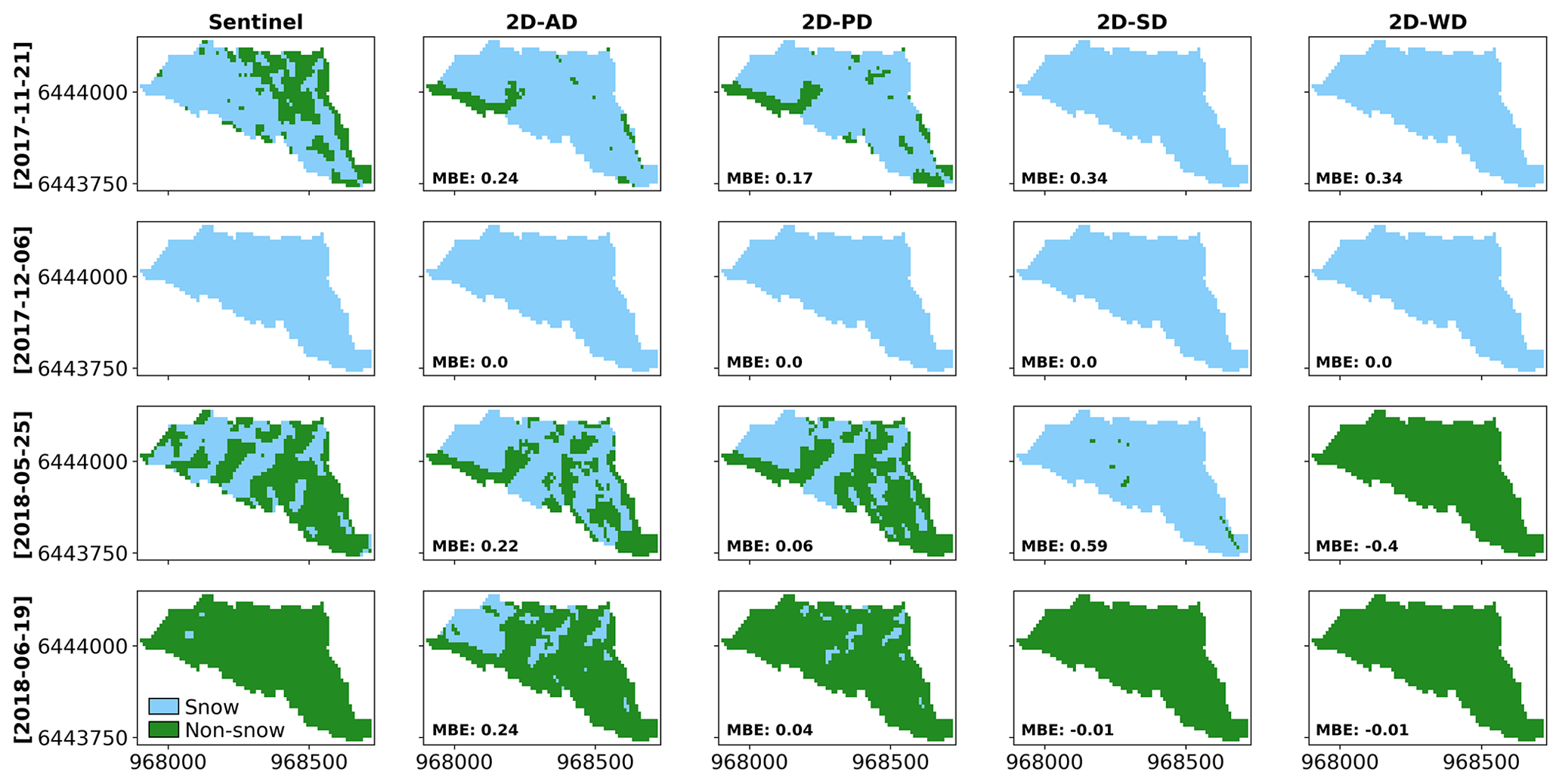
Figure 10 Snow maps for different simulations compared with the Sentinel-2 images for four cloud-free images: snow pixels (light sky blue) and non-snow pixels (green). MBE is the mean bias error between the model and Sentinel-2 image.

Table 3 Image characteristics from ESA's Sentinel-2 mission.

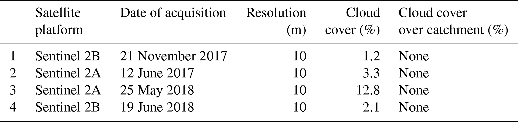
Table 4 Statistical metrics for observed and simulated parameters in different simulations (MBE: mean bias error, RMSE: root mean square error). Evapotranspiration and albedo statistics are calculated over a wind direction mask in the catchment.

The spatial distribution of snow cover during the melting period is shown for all simulations and compared to Sentinel-2 images in Fig. 10 (Table 3). On 21 November, the first snow events were followed by partial melting over the catchment (first row in Fig. 10). Our 2D-AD and 2D-PD simulations were moderately good at representing this feature, but the simulated melting was not enough overall. Apart from the upper part of the catchment, where snow distribution was not well controlled, the early snowmelt is located at the eastern edge of the catchment, a central area aligned with the river's left bank and the outlet area. The 2D-AD simulation has more snow cover than 2D-PD because of the reduced incoming radiation (caused by a reduced solar angle), which decreased the melting. On 6 December, the catchment was completely covered by snow for all simulations. It has to be noted that this date corresponds to early-season snow events when the 2D-AD and 2D-PD simulations are able to represent the snow dynamics, even for a very low snow depth. This means in particular that (1) our model spin-up initialized the ground temperature profile and its distribution well, and that (2) our distribution algorithm was well adapted, especially for snow deposition. On 25 May, the snow cover was partially melted, developing the kind of snow patches that are typical of this advanced stage of the melting season. Again, 2D-PD simulation represents the snow pixels to non-snow pixels ratio and the snow distribution (MBE = 0.06) very well. In both the Sentinel-2 image and the 2D-PD simulation, one can see some SW–NE alignment, which was slightly present on the snow distribution coefficient map (green/blue pixels on Fig. 1c); the timing of disappearance was remarkably well simulated for these pixels. The 2D-AD simulation has more snow cover than the 2D-PD simulation and Sentinel-2 image on 25 May (MBE = 0.22). However, we showed (Sect. 5.2) that 2D-AD simulation was better at simulating the snow variability and evapotranspiration compared to 2D-PD simulation. The overestimation in the 2D-AD simulation may come from the snow distribution scheme or the albedo scheme of CLM.

Table 4 shows the performance indicators for different spatio-temporal variables in the catchment. The goodness of fit for evapotranspiration is better when we distribute shortwave radiation in the catchment. The 2D-AD and 2D-SD simulations have better values of the slope, R², and RMSE. Albedo simulation was more dependent on the snow stay in the catchment. Hence, the simulation where we distributed the precipitation (2D-PD) showed better accountability in albedo simulation. The higher R² value for the albedo in 2D-WD distribution may come from the initial accumulation of a large amount of snow. However, we have shown that snow melts quite early in this simulation compared to other simulations. Finally, precipitation distribution was more important for the spatial snow cover. However, shortwave radiation influences the late melting pattern. In the Sentinel-2 images, the higher performance of 2D-PD simulation than 2D-AD may come from the precipitation distribution itself. Looking at the performance indicators together, we could see that 2D-AD was the best simulation for capturing the spatial and temporal patterns of evapotranspiration and snow cover in the catchment. This means that precipitation and evapotranspiration need to be distributed together for a more accurate representation of hydrological fluxes.

6 Discussion

The presented simulations disentangle the combined effects of the precipitation and solar radiation distributions. This makes us able to simulate a realistic patchy snow cover at 10 m resolution (Fig. 10), which is a commonly observed phenomenon over mid-elevation mountainous catchments (Revuelto et al., 2020). The lidar-based snow distribution map is particularly effective due to its accurate prediction of distributed snow depth in mountain and forest landscapes, as recently suggested (Painter et al., 2016; Hojatimalekshah et al., 2021; Jacobs et al., 2021). We moved one step ahead in using the lidar map to distribute snow precipitation over the catchment in hydrological models. The all distributed simulation (2D-AD), which encapsulates snow distribution (based on a snow map) and shortwave radiation distribution (based on the small-scale terrain), efficiently simulates the snow cover and evapotranspiration spatio-temporal dynamics in our test case. However, this simulation shows a ∼20 d delay in complete snowmelt due to reduced solar radiation when the solar angle and terrain aspect are taken into account (Fig. 9). One reason for this could be that we might slightly overestimate snow deposition when using the snow coefficient map. Indeed, the yearly spatial average amount of snow/precipitation (1442 mm) is not the same as what is measured with the gauge (1530 mm) and, at the moment, we have no means to control the average value we used in this study. This leads to an uncertainty in the cumulated snow amount that could be tuned globally with the snow coefficient map. Another reason might be the lack of melting, which could come from the snow albedo calculation in ParFlow-CLM. Indeed, looking at Fig. 9, snow aging reduces the albedo too much during winter months and gives an albedo that is too high in April, when it is re-initialized to its fresh snow value because of very small snowfall events. Those fresh snow episodes also decreased the simulated melting in the catchment during spring. Both of these defaults should be further corrected with an up-to-date snow scheme and a tuned snow coefficient map for a more precise snow depth distribution.

Our study focuses on the impact of terrain slope and aspect on the simulated spatio-temporal dynamics of snow cover and evapotranspiration in critical zone hydrological models, as this has become a debated issue in recent years (Rush et al., 2021; Parsekian et al., 2021; Fan et al., 2019). However, these are not the only sources of variability. The elevation-based precipitation distribution (Dahri et al., 2016; Avanzi et al., 2021; Jabot et al., 2012) and land-use-based spatial evapotranspiration patterns (Yan et al., 2018; Melton et al., 2021) also have a large impact on mountain hydrology and have been studied extensively in the last few decades. In the studied catchment, we considered that land-use variability was not the main driver for hydrological responses, and temperature differences within the 200 m elevation gradient were partially accounted for through the laser scan map of snow deposition. If one would like to upscale the results to larger catchments with higher land-use variability and higher elevation gradients, then temperature variability and land-use variability should be accounted for together with terrain slope and aspect.

This study shows a high sensitivity of evapotranspiration to incoming solar radiation corrections (a decrease in the regression slope from 1.55 to 1.18). In the presented results, the evapotranspiration spatial average remains larger than the observations. The reason that evapotranspiration is overestimated could come from our footprint area (Oishi et al., 2008), which is not as precise as it should be. However, it has been highlighted in many studies that comparing simulations of spatially heterogeneous variables with point observations is a difficult task (Pradhananga and Pomeroy, 2022; Zhu et al., 2021; Iseri et al., 2021). In our case, a footprint area calculation from Eddypro (Kljun et al., 2004) gave an average peak distance of ∼70 m and a 90 % contribution distance of ∼400 m for summer month daily hours. These distances are larger than the catchment width in the upwind direction and include areas that are not simulated. Moreover, the theoretical background for the footprint calculation supposes a flat terrain with a fully developed turbulent surface layer. This is not the case in our terrain, which is undulating, inducing moisture heterogeneity, with some wetlands in the lowlands. For these reasons, we chose a simpler approach for the first-order estimation of model performance, but we considered soil moisture heterogeneities through a wind direction mask (Fig. 1). We hypothesize that this spatial average is better than a single pixel for comparing simulated evapotranspiration series with observations.

ParFlow-CLM is a critical-zone physically based model that is built to closely follow the physics of hydrological processes (Kuffour et al., 2020; Tran et al., 2020). This requires reliable data for forcing, land cover, vegetation, and hydrology to keep consistency in the model framework while simulating water paths with the same accuracy. We chose to work with local observations, from which we built distributed forcing based on the presented algorithm to evaluate the model (Liston and Elder, 2006). The model calibration itself consisted of building the model (which means underground geometries and their associated parameters) only from observations. Building a model from observations was done to enhance our ability to understand the physical processes from hydrological modeling (Sidle, 2006, 2021). However, we did not have spatial observations for each pixel. We then built the model on the assumption that what we measured at a place was also valid for similar places where we did not have measurements. Available observations then restricted ranges to tune the model once we considered embedded parameterization, which explicitly solves melting and evapotranspiration via physical laws. Finally, we forced the model with reliable observed meteorological data. Using this approach, we simulated the importance of snow processes and the role of the incoming radiation distribution. Indeed, the model was evaluated against radiation budget observations (albedo), energy budget observations (latent and sensible heat fluxes), water budget terms including the snow cover, the ability of the model to produce base flow, and snowmelt timing (Table 4). Validation with Sentinel-2 images during accumulation and melting periods showed that the simulations followed the observations in terms of the onset and end of snow cover.

The last remark about the model configuration is that the domain has a no-flow boundary condition at the sides and the bottom of the domain (Chen et al., 2022; Kollet and Maxwell, 2006). This means that flux can only leave the domain through ET and streamflow. In other words, this means that larger-scale flow paths (water that enters from the sides of the domain or that gets out through the bottom of the domain) are not simulated, although they may exist for high-altitude mountainous catchments. This subsurface water transfer could also lead to small differences in outlet and evapotranspiration partitioning, but it would not change the conclusions of this study. We started some particle tracking calculations from 3D velocity fields produced by ParFlow for our simulations. They showed very weak percolation and transfer to deep horizons. Most of the water transfers occurred in the first 10 layers. This further shows that the flux leaving the bottom of the domain is not much of a concern.

The importance of critical-zone processes in improving the understanding of the hydrological cycle is strongly debated (Arora et al., 2022; Wlostowski et al., 2021). These processes often remain unexplored in large-scale hydrological models. Fan et al. (2019) recommended including the slope/aspect effect and soil depth in ESMs to improve the hydrological cycle and its feedbacks to the climate. Our study contributes to this identified issue and provides an algorithm to take into account surface heterogeneity. In this study, we detailed how the slope/aspect impacts the hydrological budget given spatial variability in the meteorological forcing along with surface to subsurface transfers, and how it can be successfully included in critical-zone hydrological modeling. The adopted algorithm efficiently captures the surface heterogeneity in the snow cover and evapotranspiration. The same algorithm also influences the spatio-temporal distributions of the snowmelt and other hydrological fluxes. The present approach involving meteorological distribution and cross-validation from field observations and Sentinel-2 remote-sensing images is also valid for subsequent years in the catchment, as will be presented in the companion paper to be published. This highlights the importance of slope, aspect, and curvature inclusion in hydrological studies.

7 Conclusions

Earth system models are gaining ample highlights in socio-economic impact studies. They include more and more processes, including the complete continental water cycle, but still face difficulty in parameterizing small-scale sub-mesh processes. These processes are crucial in the surface hydrology of mountain landscapes and their feedback to the climate. In this study, we modeled the spatial variability of the snow cover over a small mid-altitude catchment and its impact on the hydrological budget using the 3D critical-zone model ParFlow-CLM at 10 m resolution. For this purpose, we prepared distributed forcings for precipitation (mimicking snow transport), incoming solar radiation (which includes differential snow melting), and wind speed to force the model. The major conclusions of the study can be summarized as follows:

• Precipitation distribution (including wind redistribution) has the largest impact in terms of driving the patchiness of the snow cover in the catchment. This leads to snow being present for a month longer in the catchment when accounting for precipitation distribution in simulations compared to simulations ignoring it.

• Modulation of the incoming solar radiation by the local slope in the catchment is the second most influential topographic parametrization for melting as well as for evapotranspiration, which then impact the water budget of the catchment.

• Distributing wind speed according to the terrain induces some spatial variability in the simulated snowmelt at the core of the melting period but reduces this variability at the end of the melting period.

• Most hydrological processes are slope dependent, but this is barely taken into account in land surface and hydrological models. This study quantified the hydrological impacts of taking the slope effect into account (or not) in terms of melting, streamflow, and evapotranspiration dynamics. When considering the application of critical-zone models to mountainous area, we strongly recommend considering subgrid-scale slope/aspect effects in large-scale models, especially when they are used for hydrological studies. This will improve the spatial representation of snow processes and evapotranspiration and minimize biases in water resource management.