the Creative Commons Attribution 4.0 License.
the Creative Commons Attribution 4.0 License.
 | 15 May 2023
A general model of radial dispersion with wellbore mixing and skin effects
Wenguang Shi
Hongbin Zhan
Renjie Zhou
Haitao Yan
The mechanism of radial dispersion is essential for understanding reactive transport in the subsurface and for estimating the aquifer parameters required in the optimization design of remediation strategies. Many previous studies demonstrated that the injected solute firstly experienced a mixing process in the injection wellbore, then entered a skin zone after leaving the injection wellbore, and finally moved into the aquifer through advective, diffusive, dispersive, and chemical–biological–radiological processes. In this study, a physically based new model and the associated analytical solutions in the Laplace domain are developed by considering the mixing effect, skin effect, scale effect, aquitard effect, and media heterogeneity (in which the solute transport is described in a mobile–immobile framework). This new model is tested against a finite-element numerical model and experimental data. The results demonstrate that the new model performs better than previous models of radial dispersion in interpreting the experimental data. To prioritize the influences of different parameters on the breakthrough curves, a sensitivity analysis is conducted. The results show that the model is sensitive to the mobile porosity and wellbore volume, and the sensitivity coefficient of the wellbore volume increases with the well radius, while it decreases with increasing distance from the wellbore. The new model represents the most recent advancement in radial dispersion study, incorporating many essential processes not considered in previous investigations.
- Article
(2644 KB) - Full-text XML
-
Supplement
(1232 KB) - BibTeX
- EndNote


Radial dispersion refers to a process of reactive transport under the radial flow condition. One unique feature of radial dispersion (as compared to unilateral dispersion, where the flow velocity is unilateral) is that the dispersive transport becomes progressively weaker when the radial distance from the injection/pumping well becomes larger (or the radial flow velocity becomes smaller), and thus the relative importance of molecular diffusion (which is assumed to be constant) versus the dispersion becomes progressively more robust with a more significant radial distance. The radial dispersion problem is both theoretically interesting and practically important in many fields, like chemical engineering (Davis and Davis, 2002), environmental science (Reinhard et al., 1997; Chen et al., 2016), and hydrogeology (Webster et al., 1970). Although numerical modeling is probably inevitable and more powerful than the analytical modeling in describing radial dispersion, especially put forward for heterogeneous aquifers with complex initial and boundary conditions, the numerical errors and computational cost are not always trivial issues and have to be considered by the engineers. As an alternative, many analytical models have been developed for radial dispersion around an injection well under rather simplified conditions. Such analytical models can fulfill a host of tasks, such as (1) prioritizing the importance of different controlling parameters through a sensitivity analysis, (2) benchmarking the numerical solutions to elucidate the possible numerical errors such as numerical dispersion and artificial oscillation, which are notorious for advection-dominated transport problems, and (3) providing a quick screening tool before implementing a full-scale comprehensive study.
Because of the benefits mentioned above, significant efforts have been put forward over many decades in developing advanced analytical models of radial dispersion. Some examples include the works of Hoopes and Harleman (1967), Gelhar and Collins (1971), Tang and Babu (1979), Moench and Ogata (1981), Chen (1985, 1986, 1991), Hsieh (1986), Tang and Peaceman (1987), Yates (1988), Falade and Brigham (1989), Novakowski (1992), Philip (1994), Veling (2001, 2011), Huang and Goltz (2006), Chen et al. (2007, 2011, 2012, 2017), Gao et al. (2009a), Cihan and Tyner (2011), Wang and Zhan (2013), Hsieh and Yeh (2014), Zhou et al. (2017), Wang et al. (2018, 2020), Huang et al. (2019), and Li et al. (2020). A general trend of such developments is to provide more robust models that can better represent physical reality. However, despite the enormous efforts to date, some significant pitfalls still exist and become roadblocks to quick and accurate interpretation of observed data in the experiments. A primary task of this research is to eliminate such pitfalls, which are briefly illustrated in the following.
A well–aquifer system with radial dispersion comprises a wellbore, skin zone, and aquifer formation zone. The skin zone refers to the disturbed region around the well caused by drilling and construction practices or well completion (Yeh and Chang, 2013; Chen et al., 2012; Li et al., 2019, 2020; Huang et al., 2019). It is spatially between the well screen and the aquifer formation zone. Correspondingly, the injected solute may experience three processes from the wellbore to the aquifer formation zone.
Firstly, the injected solute goes through a mixing process with native (or pre-injection) water in the wellbore at the early injection stage, which is called the mixing effect. Probably due to the small radius of the well, the mixing effect has been overlooked by almost all the analytical solutions mentioned above except Novakowski (1992), Wang et al. (2018), Shi et al. (2020), and Wang et al. (2020), e.g., either by assuming that the well radius was infinitesimal or assuming that the solute concentration in the wellbore was the same as the concentration of the injected solution (Hoopes and Harleman, 1967; Veling, 2011; Zhou et al., 2017). Consequently, the solutions developed without considering the wellbore mixing effect may overestimate concentration values in both the wellbore and the aquifer (Novakowski, 1992; Wang et al., 2018; Shi et al., 2020; Wang et al., 2020). The reason is that the solute concentration in the wellbore is initially zero (when the aquifer is free of solute before the injection) and then increases steadily until it is up to the maximum, which is equal to the concentration of the injected solution.
Secondly, the solute enters the skin zone after leaving the wellbore. Compared with the aquifer formation zone of interest, the dimension of the skin zone is much smaller, e.g., ranging from 0.1 m to several meters, and it is ignored or included in the wellbore. In other words, the effect of the skin zone on radial dispersion (named the skin effect) was negligible. However, numerous previous studies demonstrated that the existence of a skin zone might significantly alter the mechanism of groundwater flow and solute transport around a well (Chen et al., 2012; Hsieh and Yeh, 2014; Yeh and Chang, 2013; Li et al., 2019, 2020). This is because the physical properties (such as permeability, porosity, or dispersivity) of the skin zone are often vastly different from their counterparts in the formation zone. Previously, studies on the skin effect mainly concentrated on the groundwater flow process around the well, and they paid less attention to solute transport processes. To date, few studies have considered the skin effect among the abovementioned analytical models on radial dispersion, such as Chen et al. (2012), Hsieh and Yeh (2014), Huang et al. (2019), and Li et al. (2020). Chen et al. (2012) proposed an analytical solution of solute transport with the skin effect to investigate the influences of dispersivity on radial dispersion; soon after, Hsieh and Yeh (2014) extended the model of Chen et al. (2012) by taking into account a third type (Robin) of condition. Huang et al. (2019) demonstrated that the skin effect significantly influences observed breakthrough curves (BTCs) for radially convergent tracer tests. Recently, Li et al. (2020) developed an analytical model for radial reactive transport with the skin effect to investigate the impacts of dispersivity, effective porosity, and mass transfer coefficient in the skin zone on radial dispersion. The abovementioned studies demonstrated that the skin effects are significant for radial dispersion.
Thirdly, the solute moves into the formation zone from the skin zone by advective, diffusive, and dispersive processes. Such processes have been widely described by the traditional advection–dispersion equation (ADE) which is based on Fick's law; however, many recent studies demonstrated that the ADE model mainly worked well for homogeneous (or nearly homogeneous) porous media. As for reactive transport in heterogeneous media, the BTCs may exhibit a host of non-Fickian characteristics, such as early arrival and heavy tailing (Di Dato et al., 2017; Molinari et al., 2015). Alternatively, many non-Fickian transport models have been developed, such as the multirate mass transfer model (MRMT) (Le Borgne and Gouze, 2008; Haggerty et al., 2001; Guo et al., 2020), the mobile–immobile model (MIM) (van Genuchten and Wierenga, 1976; Zhou et al., 2017; Wang et al., 2020), continuous-time random-walk (CTRW) models (Dentz et al., 2015; Hansen et al., 2016), fractional-derivative ADE (fADE) models (Soltanpour Moghadam et al., 2022; Chen et al., 2017), a combination of MRMT and CTRW (Kang et al., 2015), and so on (Zheng et al., 2019; Lu et al., 2018). Although the models of MRMT, CTRW, and fADE perform well in modeling non-Fickian transport, it is not easy to obtain the analytical solutions of these models. Meanwhile, these theories are usually not easy to apply when solving regional-scale transport problems, as pointed out in a recent study (Zheng et al., 2019). MIM is an extension of ADE by considering both flowing and stagnant regions in porous media and mass transfer between them (van Genuchten and Wierenga, 1976; Zhou et al., 2017; Wang et al., 2020). Zhou et al. (2017) and Wang et al. (2020) derived the MIM solutions of radial dispersion. However, the skin effect and the scale effect were ignored in their studies, which will be investigated in this study. Besides the MRMT, MIM, CTRW, and fADE models, another approach to representing the heterogeneity is to use a scale-dependent dispersivity (or dispersion) in the ADE or MIM models (Haddad et al., 2015; Gelhar et al., 1992). Gao et al. (2009a) and Chen et al. (2007) discussed radial dispersion and found that the scale-dependent dispersion effect was not negligible. There is also experimental evidence for the scaling of dispersion, mixing, and reaction (Leitão et al., 1996; Edery et al., 2015).
The differences among the currently available analytical solutions for radial dispersion have been reviewed and summarized in Table 1. As one can see from this table, the mixing effect in the wellbore was ignored in all of the models except for Novakowski (1992), Wang et al. (2018, 2020), and Shi et al. (2020). Only Chen et al. (2012), Hsieh and Yeh (2014), Huang et al. (2019), and Li et al. (2020) took the skin effect into account. The differences among the solutions of Tang and Babu (1979), Moench and Ogata (1981), Hsieh (1986), Tang and Peaceman (1987), Yates (1988), Cihan and Tyner (2011), and Chen et al. (2011) mainly consist of the boundary conditions, source-injection types (instantaneous or continuous), and initial conditions.
Table 1Summary of the current models for the radial dispersion around the recharge well.
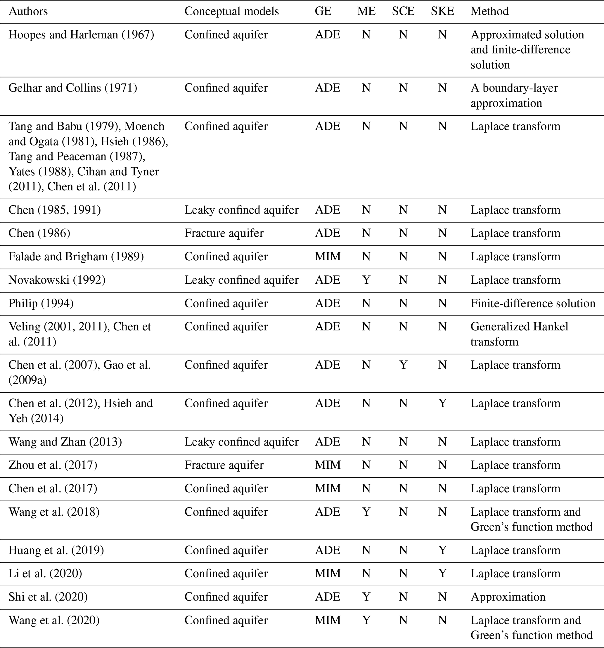
Note: “GE”, “ME”, “SCE”, and “SKE” represent governing equation, mixing effect, scale effect, and skin effect, respectively. “Y” and “N” represent whether the effect is considered or not.
In summary, no existing analytical model has ever considered the mixing, skin, scale, and media heterogeneity effects (which are described using MIM) simultaneously. Although the numerical method is more powerful than the analytical method for problems with complex initial and boundary conditions and heterogeneous aquifers of interest, numerical errors could not be avoided easily for the MIM models of concern here, such as numerical dispersion and numerical oscillation issues (Zheng and Wang, 1999; Wang and Zhan, 2013). Meanwhile, the analytical solutions are usually computationally more efficient than the numerical solutions and can be easily coupled into optimization algorithms for problems related to parameter estimation (Neuman and Mishra, 2012). Therefore, a primary purpose of this study is to develop such an analytical model. Furthermore, the accuracy and robustness of the developed model will be tested against a finite-element numerical simulation and experimental data. Moreover, a sensitivity analysis will be conducted to prioritize the influences of various controlling parameters on the newly developed radial dispersion reactive transport model.
2.1 Mathematical model of radial dispersion
An aquifer is assumed to be confined, homogeneous, horizontally isotropic, have a constant thickness, and be fully penetrated by a well from which the solute is injected. A cylindrical coordinate system is established with the r axis horizontal and the z axis vertically upward. The origin of the coordinate system is located at the intersect of the well center and the middle elevation of the aquifer. A schematic diagram of the problem is available in Fig. S1 in the Supplement.
In this study, we mainly focused on developing analytical solutions of radial dispersion with a Heaviside step source (or step function for short hereinafter), as solutions of a variety of injection scenarios can be easily obtained based on such a step source solution, as shown in Eq. (S2), Eqs. (4a, b), or Eqs. (5a, b). Assuming that tinj is the duration of the step source, the solute source concentration (C0) is Cinj(t) when time is smaller than tinj, while it is Ccha(t) when time is greater than tinj, in which Cinj(t) and Ccha(t) represent the solute concentrations (M L−3) in the wellbore before time tinj and after time tinj, respectively. When Ccha(t)=0 and tinj approach zero but the total injected mass remains finite, the model of the step source reduces to the model of the instantaneous injection. Similarly, the model of the step source becomes the model of the continuous injection source when tinj becomes infinity.
Similar to Chen et al. (2012) and Hsieh and Yeh (2014), a two-region (skin and formation) model of radial dispersion is employed to describe the skin effect. In the skin zone, the governing equations of radial dispersion are
In the formation zone, one has
where the subscripts “m” and “im” refer to parameters in the mobile and immobile domains, respectively. The subscripts “1” and “2” refer to parameters in the skin and formation regions, respectively. and are the mobile and immobile concentrations (M L−3) of the skin zone, respectively. and are the mobile and immobile concentrations (M L−3) of the formation zone, respectively. r is the radial distance (L) from the center of the well. rw is the well radius. rs is the radial distance (L) from the center of the well to the outer boundary of the skin zone. va is the average radial pore velocity (L T−1) in the aquifer. and ; and represent Darcian velocities (L T−1) in the skin and formation zones, respectively. α1 and α2 represent the longitudinal dispersivities (L) in the skin and formation zones, respectively. , , , and are reaction rates for the first-order reaction rate, the first-order biodegradation, or the radioactive decay (T−1). , , , and are porosities. , , , and are retardation factors (dimensionless). ω1 and ω2 represent the first-order mass transfer coefficients (T−1) between the mobile and immobile dissolved phases in the skin and formation zones, respectively. One point to note is that the molecular diffusive effect is assumed to be negligible in the above governing equations.
Assuming that the skin and formation zones are initially free of solute, the initial conditions are
The outer boundary condition at an infinite distance is
Two types of models have been widely applied to the boundary condition at the well screen: the mass flux continuity (MFC) model and the resident concentration continuity (RCC) model. The RCC model is
and the MFC model is
where and refer to velocities in the injection and chasing phases, respectively. It was demonstrated that the mass balance requirement could not be satisfied in the RCC model, while the resident concentration was not continuous in the MFC model (Wang et al., 2018). Many experimental studies demonstrated that the MFC model performed better than the RCC model (Novakowski, 1992). Therefore, the MFC model will be used to describe the boundary condition in the wellbore in this study. Comparing Eqs. (4) and (5), one may find that the main difference between these two models is whether the dispersivity is involved or not. Recently, Wang et al. (2019) pointed out that the conflicts between these two models could be resolved by a scale-dependent dispersivity, which was zero at the well screen and increased with the travel distance of the solute. This is because when the dispersivity is zero in Eqs. (5a) and (5b), the MFC model reduces to the RCC model. The model of the scale-dependent dispersivity will be discussed in Sect. 2.4.
When taking into account the mixing effect in the wellbore, one has
where Vw,inj is the volume (L3) of water in the wellbore when t≤tinj, and . hw,inj is the water level (L) in the wellbore when t≤tinj. , B is the thickness (L) of the aquifer, Vw,cha is the volume (L3) of water in the wellbore when t>tinj, and . hw,cha is the water level (L) in the wellbore when t>tinj, is the velocity at the well screen in the injection phase, and . is the velocity at the well screen in the chasing phase, and it equals . Qinj and Qcha are the well flow rates (L3 T−1) in the injection and chasing phases, respectively. The mass balance for the well in Eqs. (6) and (7) is only relevant when velocity exceeds zero because it does not contain terms for possible diffusive losses.
The water level in the wellbore (e.g., hw,inj and hw,cha) could be determined by solving the groundwater flow model. In the steady state, one has
where K is the hydraulic conductivity (L T−1), and ; K1 and K2 are the hydraulic conductivities (L T−1) of the skin and formation zones, respectively.
By conducting the integration on Eqs. (8) and (9) from rw to rs and from rs to re, respectively, the water level in the wellbore can be obtained as follows:
where re is the radial distance (L) from the center of the well to the outer boundary of the formation zone, and h0 is the hydraulic head (L) at re. One could find that a finite radius re is needed to keep hw finite. It seems to contradict the boundary condition of the transport problems, which is at infinity, as shown in Eq. (3). The reason for such a “contradiction” could be explained as follows. In reality, the influence area is limited by the finite injection rate and the finite injection time of the well (from a plane-view perspective), bounded by a circle with a radius re where the hydraulic head is almost constant and the flow velocity is almost zero.
At the interface between the skin and formation zones, the concentration and dispersive flux have to be continuous, and one has
Since Darcy fluxes (advective solute fluxes) are continuous, dispersive fluxes must be continuous, which is Eq. (13).
Here, it is worthwhile to comment on the nature of using the MIM approach to describe transport in heterogeneous aquifers. First, it has been commonly observed that the aquifer heterogeneity renders the use of ADE invalid in many cases, as ADE is developed and used primarily for homogeneous aquifers. In particular, ADE fails to explain the early breakthrough and long tailing phenomena that are frequently observed in transport in heterogeneous aquifers, as illustrated in the introduction. Second, a striking feature of a heterogeneous aquifer is that a sequence of mobile and less mobile regions coexists. In contrast, a homogeneous aquifer may be simplified as a single (mobile) region. Ideally, suppose one knows precisely the spatial distribution of those mobile and less mobile regions and their associated flow and transport parameters. In that case, one can use a high-resolution numerical simulator to predict the flow and transport process precisely. Unfortunately, this is not feasible for most practical cases. Therefore, as an alternative, we have adopted the concept of the MIM approach in which two continuums consisting of a mobile domain and an immobile domain coexist over the entire heterogeneous aquifer. Each of these two continuums has uniform flow and transport parameters (such as porosity or retardation factor) for the sake of simplification. Furthermore, mass can transfer between these two continuums in a certain fashion, usually using the first-order rate-limited equation. Third, this alternative approach has successfully explained many phenomena that cannot be explained using ADE, for instance, the early breakthrough and long tailing issues. Later, the two-continuum MIM approach was expanded to multiple-continuum MIM or multirate MIM approaches to better capture the transport features in a heterogeneous aquifer (Vangenuchten and Wierenga, 1976; Elenius and Abriola, 2019; Guo et al., 2019). In summary, the MIM does not incorporate the spatial variation of flow and transport parameters that are mostly unknown. Instead, it is based on an alternative approach, using two or more interrelated continuums, and in each continuum, the flow and transport parameters remain uniform over space. To date, the validation of the MIM model has been tested by numerous experimental studies (Griffioen et al., 1998; Gao et al., 2009b; Elenius and Abriola, 2019).
2.2 Solution of radial dispersion
In this study, dimensionless forms of parameters used in the derivation of analytical solutions are defined as , , , , , , , , , , , , , , , , and .
The detailed derivation of the analytical solution in the Laplace domain can be seen in Sect. S1 in the Supplement. The analytical solution is
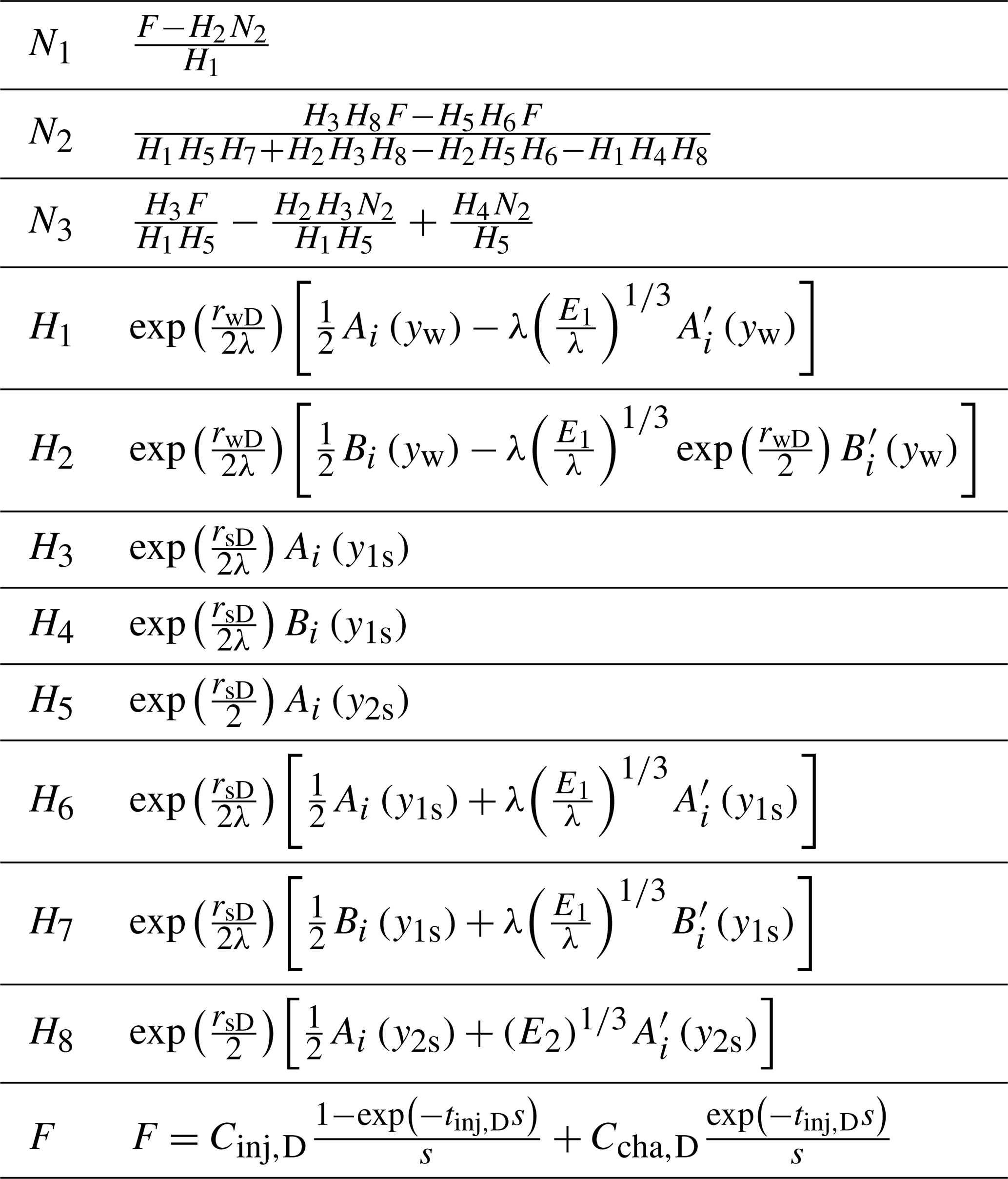
where Ai(⋅) and Bi(⋅) are the Airy functions of the first and second kinds, respectively. Cinj,D and Ccha,D can be determined by Eqs. (S18) and (S19), which can be seen in Sect. S1. and are the derivatives of the Airy function of the first and second kinds, respectively. , , , , , , , , , , , , , and . s is the dimensionless Laplace transform parameter in respect to dimensionless time tD. The expressions for N1, N2, and N3 are listed in Table 2.
Table 2Expressions of coefficients in solutions of Eqs. (14a)–(15b).
From Eqs. (14) and (15), one may find that it is not easy to invert the Laplace-domain solution to obtain the real-time solution analytically. Alternatively, numerical Laplace transform techniques such as the Fourier series method (Dubner and Abate, 1968), Zakian method (Zakian, 1969), Schapery method (Schapery, 1962), de Hoog method (De Hoog et al., 1982), and Stehfest method (Stehfest, 1970) are called in, where the de Hoog and Stehfest methods perform better for problems related to radial dispersion (Wang and Zhan, 2015). In this study, the MATLAB script of the de Hoog method compiled by Hollenbeck (1998) will be employed to facilitate the computation of the inverse Laplace transform, where the numerical tolerance is set to .
2.3 Special cases of the new solution
The new solution of this study considers the mixing effect, skin effect, and media heterogeneity (which is described using MIM) simultaneously, and the solute is injected into the well as a step source. This general solution encompasses many previous studies as special cases. For instance, when rs→∞, the skin effect is excluded. tinj→∞ implies that the solute is continuously injected into the well. tinj→0 means that the solute is instantaneously injected into the well. ω=0 implies that the MIM solution reduces to the ADE solution. or rw=0 shows that the mixing effect is excluded.
Therefore, the new solution reduces to the solutions of Hoopes and Harleman (1967), Gelhar and Collins (1971), Tang and Babu (1979), Moench and Ogata (1981), Hsieh (1986), Tang and Peaceman (1987), and Philip (1994) when rs→∞, tinj→∞, ω=0, and . The solution of Wang et al. (2018) is a special case of this study when rs→∞, tinj→∞, and ω=0.
2.4 Extension of the new solution with scale-dependent dispersivity
Due to the heterogeneities of the porous media, the dispersivity was found to be dependent on the travel distance of the solute from the source, and such a phenomenon was first observed in the field-scale experiment (Dagan, 1988; Gelhar et al., 1992; Pickens and Grisak, 1981a). The field-scale effect (i.e., dispersivity growing with distance from the well) is usually considered to be a result of spatial heterogeneity at different scales in the aquifer. Subsequently, the scale-dependent dispersivity phenomenon was also found in controlled laboratory tests due to heterogeneities caused by the bridging effect and microstructures, although the sediments (as the porous media) are well sorted and carefully packed (Silliman and Simpson, 1987; Berkowitz et al., 2000; Wang et al., 2019; Gao et al., 2010). For example, Silliman and Simpson (1987) found that the dispersivity continuously increased with distance, based on the experiments conducted in a m sandbox. Berkowitz et al. (2000) obtained similar conclusions to Silliman and Simpson (1987) in the laboratory-controlled experiment. Wang et al. (2019) also concluded that the scale-dependent model performed better than the scale-independent model in interpreting observed BTCs of the laboratory-controlled experiment. To date, four types of functions have been widely used to describe scale-dependent dispersivity, including asymptotic, parabolic, exponential, and linear functions, as summarized by Pickens and Grisak (1981b). In this section, the model of the scale-independent dispersivity (e.g., Eqs. 14 and 15 in Sect. 2) will be extended by considering the linear-asymptotic dispersivity model in the formation zone. As for the other types of scale-dependent functions, the analytical solutions could be derived using a similar approach. The formula of the linear distance-dependent dispersivity is
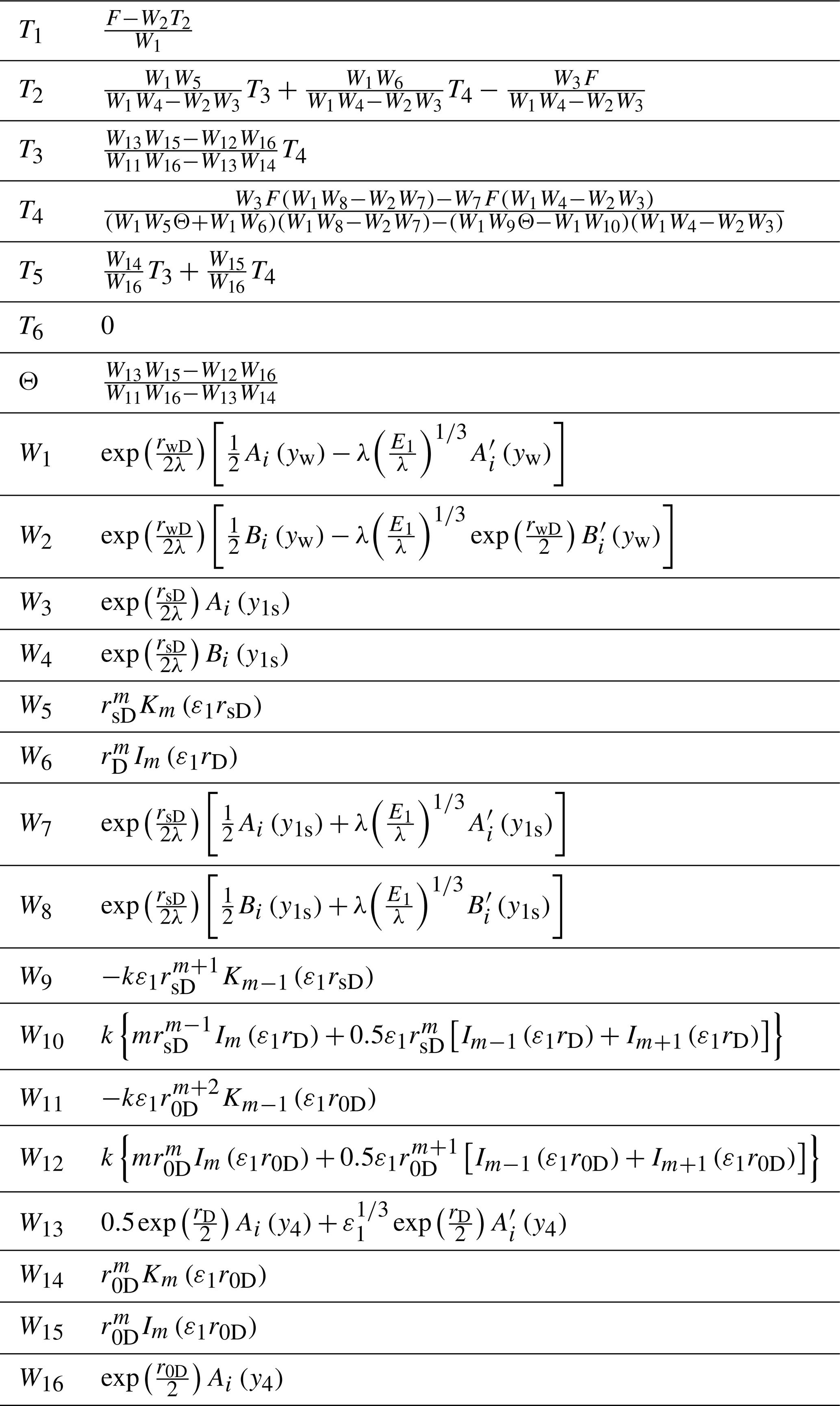
where r0 is the distance (L), α2(r0)=α0, k is a constant (dimensionless), and the modified solutions are
where , Km(⋅) is the mth-order modified Bessel function of the second kind, and Im(⋅) is the mth-order modified Bessel function of the first kind. The expressions for T1, T2, T3, T4, T5, and T6 are listed in Table 3. , , Cinj,D, and Ccha,D can be determined by Eqs. (S34)–(S36), and the detailed derivation of Eqs. (17) and (18) can be seen in Sect. S2.
Table 3Expressions of coefficients in solutions of Eqs. (17a)–(18c).
Substituting Eq. (16) into the dispersivity coefficient (Dα), one has
where D0 is the molecular diffusion coefficient (L2 T−1). A few interesting features are notable here. First, because of the unique feature of a divergent flow field in which the velocity is inversely proportional to the radial distance and the use of a dispersivity function that is proportional to the radial distance when r≤r0, the dispersion coefficient in Eq. (19) actually becomes constant. However, one must be aware that if other types of dispersivity equations are used (such as exponential and parabolic functions), the dispersion coefficient in Eq. (19) will depend on the radial distance from the well. Second, even when Dα becomes constant for a linear dispersivity function when r≤r0, the mechanical dispersion is still dominant since the value of D0 is generally much smaller than the mechanical dispersion term of . For instance, the diffusion coefficient in water ranges from to m2 s−1, and it is much smaller in the porous media (Freeze and Cherry, 1979). When k=0.01, Q=0.1 m3 s−1, B=1 m, and , one has m2 s−1. Therefore, it is reasonable to ignore the molecular diffusion effect when r≤r0. The values of are dependent on k. The chosen value of k=0.01 is from experimental studies, for instance, k=0.018 in Chen et al. (2007) and k=0.024 and 0.013 in this study, as shown in Table 5.
2.5 Extension of the new solution to a leaky confined aquifer
Regardless of Eqs. (14) and (15) or Eqs. (17) and (18), the aquifer is assumed to be completely isolated from the underlying and overlying aquitards (strictly confined), which might not be true in real applications. As stated before (Zhan et al., 2009a, b), it is nearly impossible to maintain a strictly confined condition in terms of transport. This is because as long as a solute in the aquifer is in contact with the upper or lower aquitard, molecular diffusion will always drive the solute from a high-concentration aquifer into the solute-free aquitard, even if the cross-formation flow in the aquitard does not exist. In fact, such diffusion-driven transport of a solute into the aquitard and the subsequent back-diffusion (from aquitard to aquifer when the aquifer solute concentration drops below the solute concentration in the aquitards) is responsible for many long tails in aquifer BTCs. The importance of aquitards in regulating solute transport has indeed been recognized by a number of investigators, such as Chen (1985, 1986, 1991), Yates (1988), Novakowski (1992), Q. Wang and Zhan (2013), and Zhou et al. (2017).
In this section, the solutions of Eqs. (14) and (15) will be extended considering underlying and overlying aquitards. The detailed derivation of the analytical solution in the Laplace domain can be seen in Sect. S3.
In the aquifer, the solutions are
In the aquitards, the solutions are
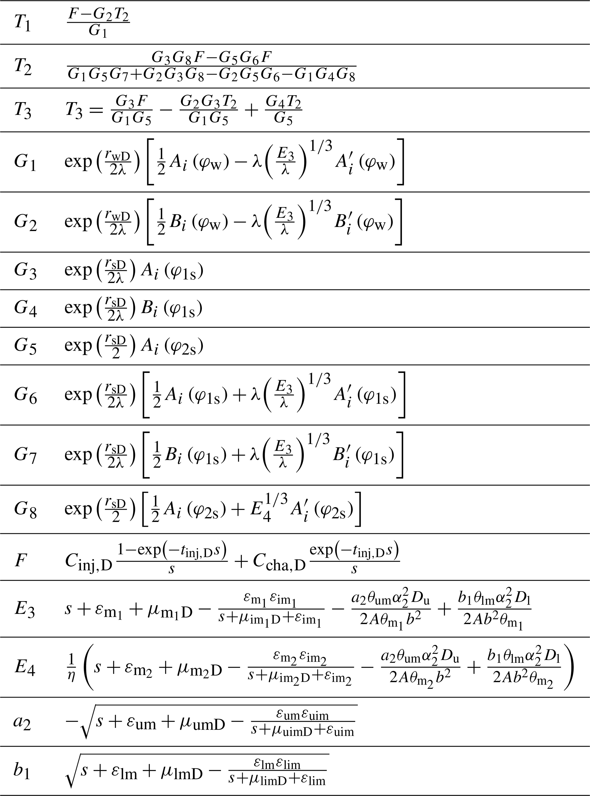
where the letters “u” and “l” in the subscripts represent the upper and lower aquitards, respectively, , , , , and . The expressions for a2, b1, T1, T2, and T3 are listed in Table 4. Cinj,D and Ccha,D can be determined by Eqs. (S71) and (S72), which can be seen in Sect. S3.
Table 4Expressions of coefficients in solutions of Eqs. (20a)–(23c).
The solutions of Chen (1985, 1986, 1991) and Yates (1988) are special cases of this study when rs→∞, tinj→∞, ω=0, and . When rs→∞, tinj→∞, and , the new solution reduces to the solution of Zhou et al. (2017). Novakowski (1992) considered the wellbore mixing effect in an aquifer–aquitard system, while he ignored other factors such as the skin effect, scale-dependent dispersivity, and mass transfer between the mobile and immobile domains in porous media.
3.1 Test of new solutions
To test the new solution of this study, a numerical simulation based on the Galerkin finite-element method is conducted in the COMSOL Multiphysics platform. More details about the numerical simulation setup can be seen in Sect. S4. The parameters used in the numerical simulation are rw=2.5 cm, rs=12.5 cm, mL s−1, tinj=300 s, α1=2.5 cm, α2=2.5 cm, θm=0.30, θim=0.01, ω=0.001 d−1, , B=50 cm, s−1, and . These parameters are from the experimental applications of Chao (1999), Chen et al. (2017), and Wang et al. (2018, 2020), in which Wang et al. (2020) summarized the values of reaction rate, retardation factor, dispersivity, porosity, and first-order mass transfer coefficient for sand and clay used in numerous investigations, as shown in Table 4 of Wang et al. (2020). In addition, the values of the retardation factor and reaction rate show that the chemical reaction and sorption are weak for the tracer of potassium bromide (KBr) in the experiment of Chao (1999). This is unsurprising since KBr is commonly treated as a “conservative” tracer.
As it is difficult to describe the wellbore mixing effect in COMSOL Multiphysics, the wellbore concentration is computed by the analytical solutions of Eqs. (14) and (15). Figure 1a and b show the comparison of concentration between the numerical and analytical solutions of this study, and good agreement between these two kinds of solutions is evident for different times and locations. The comparisons between the numerical solution and analytical solutions of Eqs. (20)–(23) are shown in Sect. S4.2, and the agreement is also good between them.
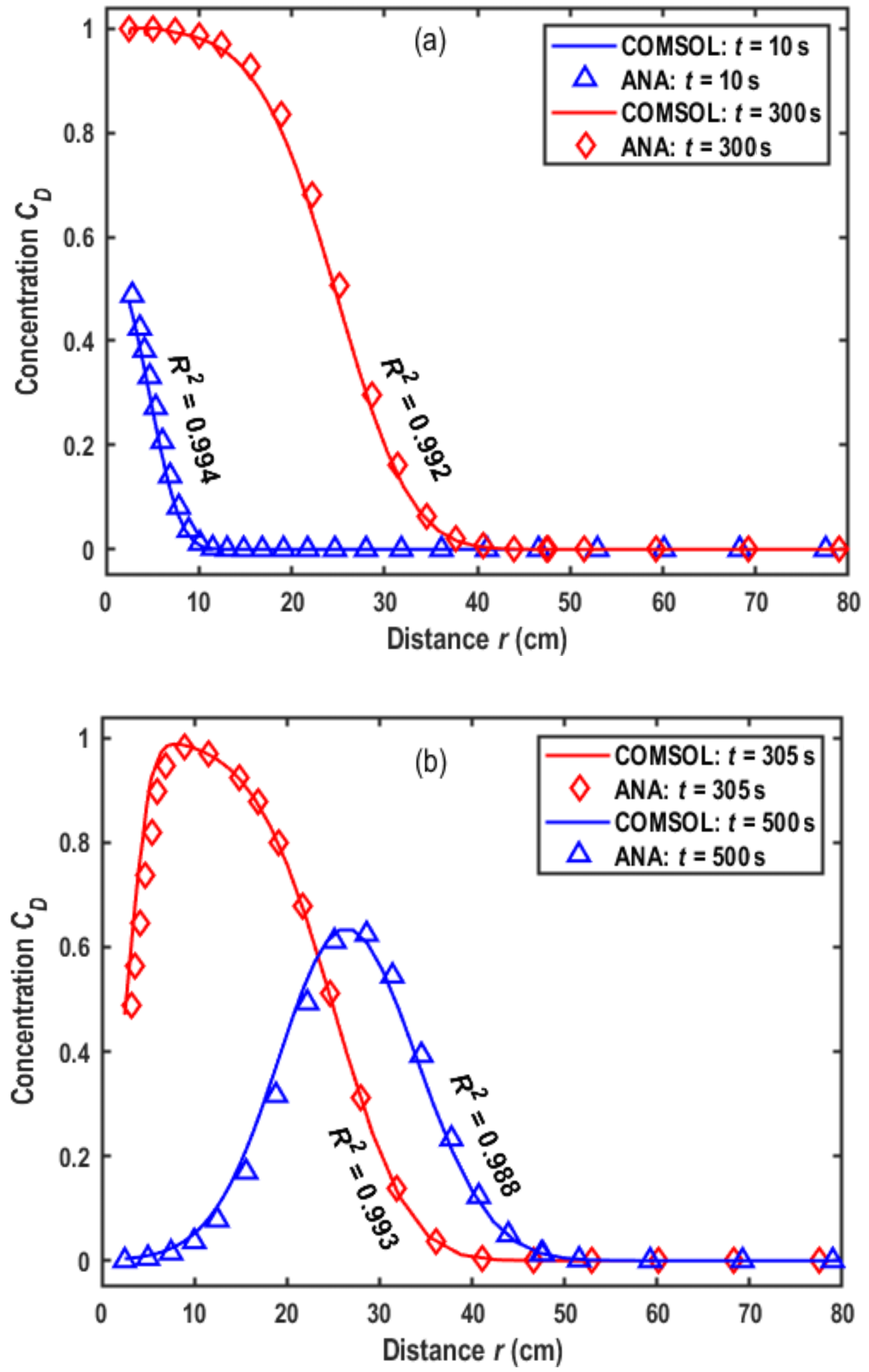
Figure 1Comparison of the numerical solution by COMSOL Multiphysics and the analytical solution of this study for different times. (a) In the injection phase; (b) in the chasing phase.
3.2 Test of the model using experimental data
To test the influence of the mixing effect, skin effect, scale effect, and heterogeneity of the media on radial dispersion, the experimental data of Chao (1999) are employed. Chao (1999) reported a laboratory experiment of radial dispersion in a sand tank 244 cm in length, 122 cm in width, and 6.35 cm in depth. A well with a radius of 1.0 cm fully penetrated a confined aquifer. Two observation wells were, respectively, located 22.5 cm and 30.4 cm away from the well center. KBr is chosen as a conservative tracer. Before the tracer is introduced into the wellbore, a steady-state flow field is produced by injecting KBr-free water into the aquifer with a constant injection rate of 9.9 mL min−1. The injection time is 5 h (tinj=300 min) for the tracer while maintaining the same injection rate of 9.9 mL min−1. The experimental data of Chao (1999) were interpreted by Gao et al. (2009a) using the model of Chen et al. (2007), as shown in Fig. 2. “SDM” and “CDM” in the legend of Fig. 2 refer to the scale-dependent dispersivity model and the constant dispersivity model, respectively. Chen et al. (2007) approximated the injection as an instantaneous source (the validity of such a treatment will be addressed later), and the mass M of the instantaneous injection is calculated by
The other parameters of the analytical solution are listed in Table 5. The parameters estimated by Gao et al. (2009a) are also included in Table 5 for comparison. One may find that the goodness of fit between the observed data and the models of Gao et al. (2009a) and Chen et al. (2007) seems good at the observation point close to the well, but they could not capture BTCs at r=30.4 cm. This is probably for the following two reasons. Firstly, the model of Chen et al. (2007) used to best fit the data is an instantaneous slug test model, which is a rather gross approximation of the injection, which lasted about 5 h. A more proper way is to treat the 5 h injection as a step source. Secondly, the solution of Chen et al. (2007) only considered the scale-dependent dispersivity but ignored the mixing effect and the mass transfer between the mobile and immobile domains.
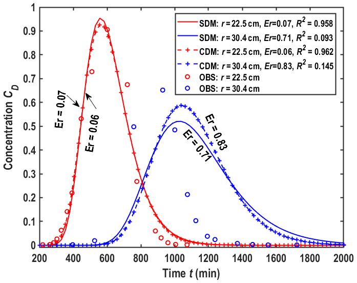
Figure 2Fitness of observed BTC by the solution of Chen et al. (2007) which considers the scale effect but ignores the mixing and skin effects.
Table 5Parameter values used in Figs. 2 and 3.
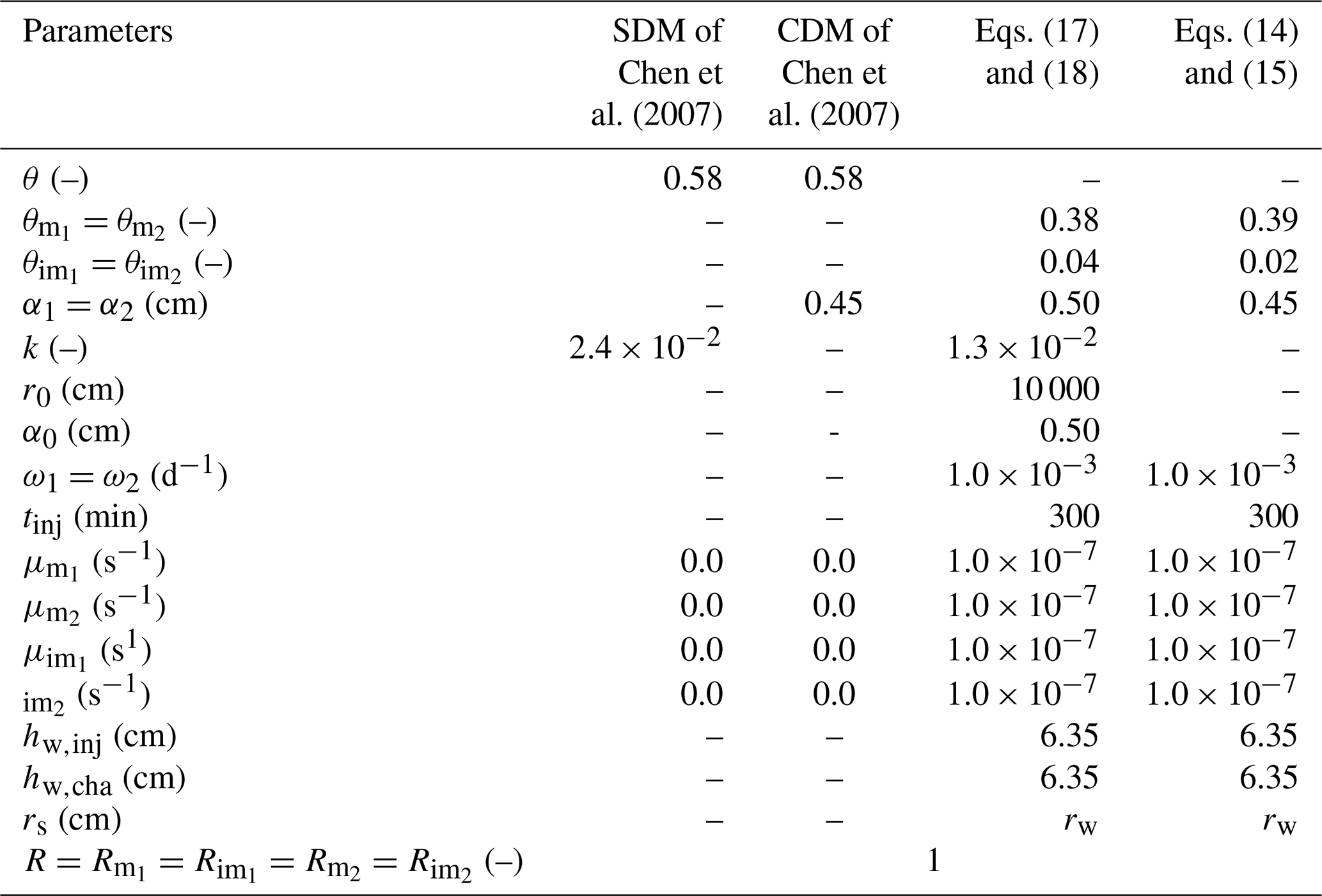
Note: “SDM” represents the scale-dependent dispersivity model. “CDM” represents the constant dispersivity model. “–” in units represents that the variable is dimensionless. “ – ” represents that the variable is not included in the model.
To test the new solutions of this study, we try to best-fit the observed data again using the newly developed model considering the scale-dependent dispersivity, mixing effect, and heterogeneity of the media (described using MIM). As there is no aquitard in the controlled laboratory experiment, the aquitard effect is irrelevant. Meanwhile, as there is no skin, the skin effect is not included either. The best fitness between the analytical solution and the experimental data is an optimization process by minimizing the “error” between them:
where COBS and CCOM represent the observed and computed concentrations, respectively, Er is the error, and N is the number of sampling points. In this study, the genetic algorithm (GA) is employed to search the optimal parameter values, such as , α1, and ω1 for CDM of Eqs. (14) and (15) and , α0, k, and ω1 for SDM of Eqs. (17) and (18). GA is a stochastic search method based on natural selection and is preferred for optimization. Meanwhile, GA has been packaged into the MATLAB toolbox (Katoch et al., 2020; Whitley, 1994; Deb et al., 2002), and therefore it is efficient, simple to program, and robust. The estimated values of some key parameters are listed in Table 5. The errors between the observed and computed BTCs by different models are listed in Table 6. Figure 3 shows the fitness between the analytical solution and experimental data, with and without scale-dependent dispersivity, respectively. As GA converges after 500 generations (iterations), the fitness is good, as shown in Fig. 3, and the estimated parameters are physically sound.
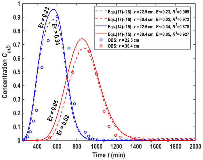
Figure 3Fitness of observed BTCs by new solutions of this study, where Eqs. (14) and (15) are without the scale effect and Eqs. (17) and (18) are with the scale effect, respectively.
Table 6Errors between observed and computed BTCs in Figs. 2 and 3.
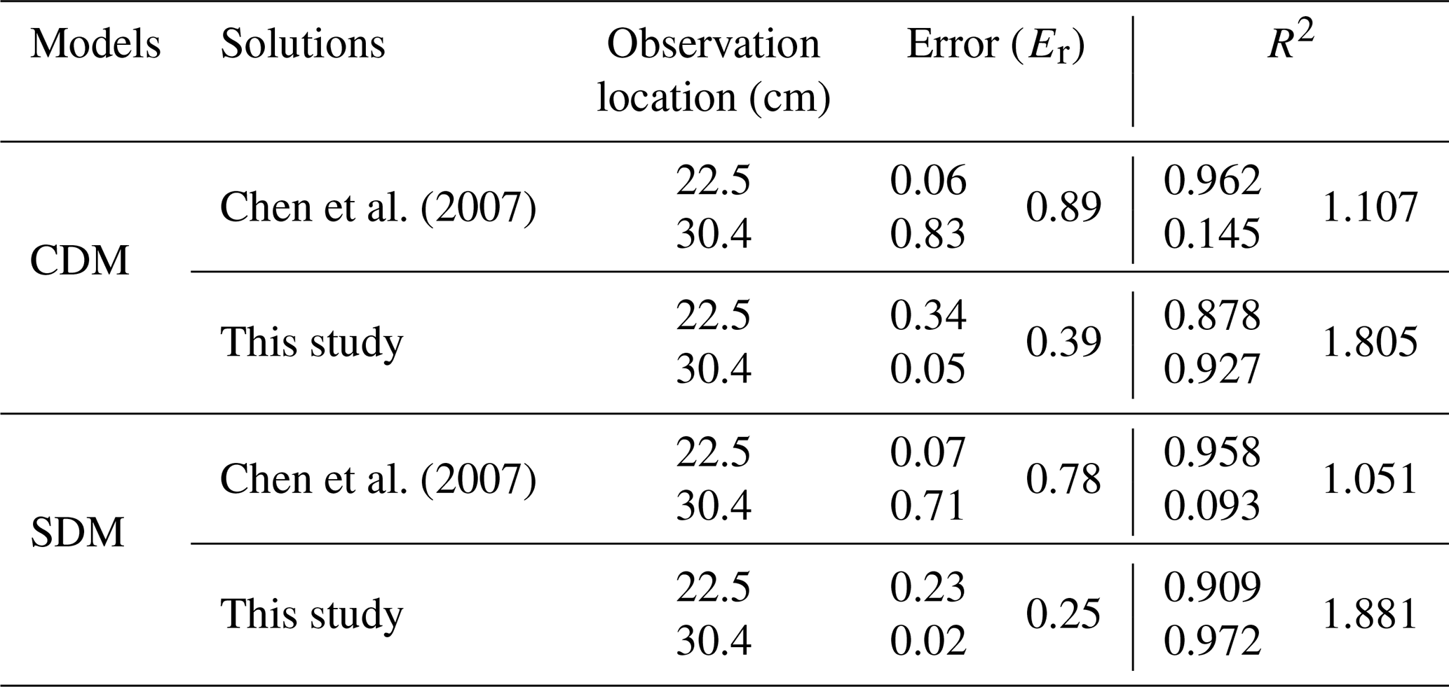
Comparing Figs. 2 and 3 shows that the solutions of this study perform better than the model of Chen et al. (2007), since the fitness is good for both observation locations. To better evaluate the overall performance of the models for both locations, we have used Eq. (25) and the coefficient of determination (R2) to compute the errors of best fitness with two BTCs simultaneously in Figs. 2 and 3, and R2 is defined by
where is the average concentration of observed data. The results are listed in the last two columns of Table 6. This table shows that the new model performs better. For example, when using CDM, the overall errors for the best-fitting two locations are 0.89 (which is the summation of 0.06 and 0.83 in Table 6) for Chen et al. (2007) and 0.39 (which is the summation of 0.34 and 0.05 in Table 6) for this study. When using SDM, however, the overall errors for the best-fitting two locations are 0.78 for Chen et al. (2007) and 0.25 for this study. The overall R2 shows the same observation as the overall Er, where the overall R2 is closer to 2, implying that the model precision is much higher. Evidently, the model with the scale effect is the best choice for interpreting the experimental data.
We must emphasize that better fitting of one model than the other with the experimental data should not be used as the only evidence of proof of model performance. This is because a model with more fitting parameters usually performs better than the model with fewer fitting parameters. Besides the best-fitting exercises, however, one should pay more attention to see whether the model adequately acknowledges the underlying physiochemical principles governing the transport processes. As far as we can see, the new model proposed in this study has honored the underlying physiochemical principles governing the radial dispersion process properly. In addition, the model performance (as reflected in the best-fitting practice with the experimental data) is also considerably better. Therefore, based on these two considerations, the new model of this study can be regarded as a significant advancement of present knowledge on radial dispersion. Furthermore, the new model is quite general and encompasses almost all the existing models as subsets.
3.3 Sensitivity analysis
As the new model involves several controlling parameters, it is necessary to prioritize the importance of these parameters in their control on the model performance. In this study, a sensitivity analysis involving normalized parameters is conducted as follows (Kabala, 2001; Yang and Yeh, 2009):
where SCi,j is the sensitivity coefficient of the jth parameter Ij at the ith time. Ci is the concentration at the ith time. Ij represents any one parameter of interest, like the volume of water in the wellbore (Vw), k, , , and so on. A larger |SCi,j| value means a higher sensitivity.
As the expression of the new analytical solution is complex, it is not easy to get the values of SCi,j directly from Eq. (27). Therefore, a finite-difference scheme is used alternatively to approximate the right-hand-side term (Kabala, 2001; Yang and Yeh, 2009):
where ΔIj is a small increment of Ij.
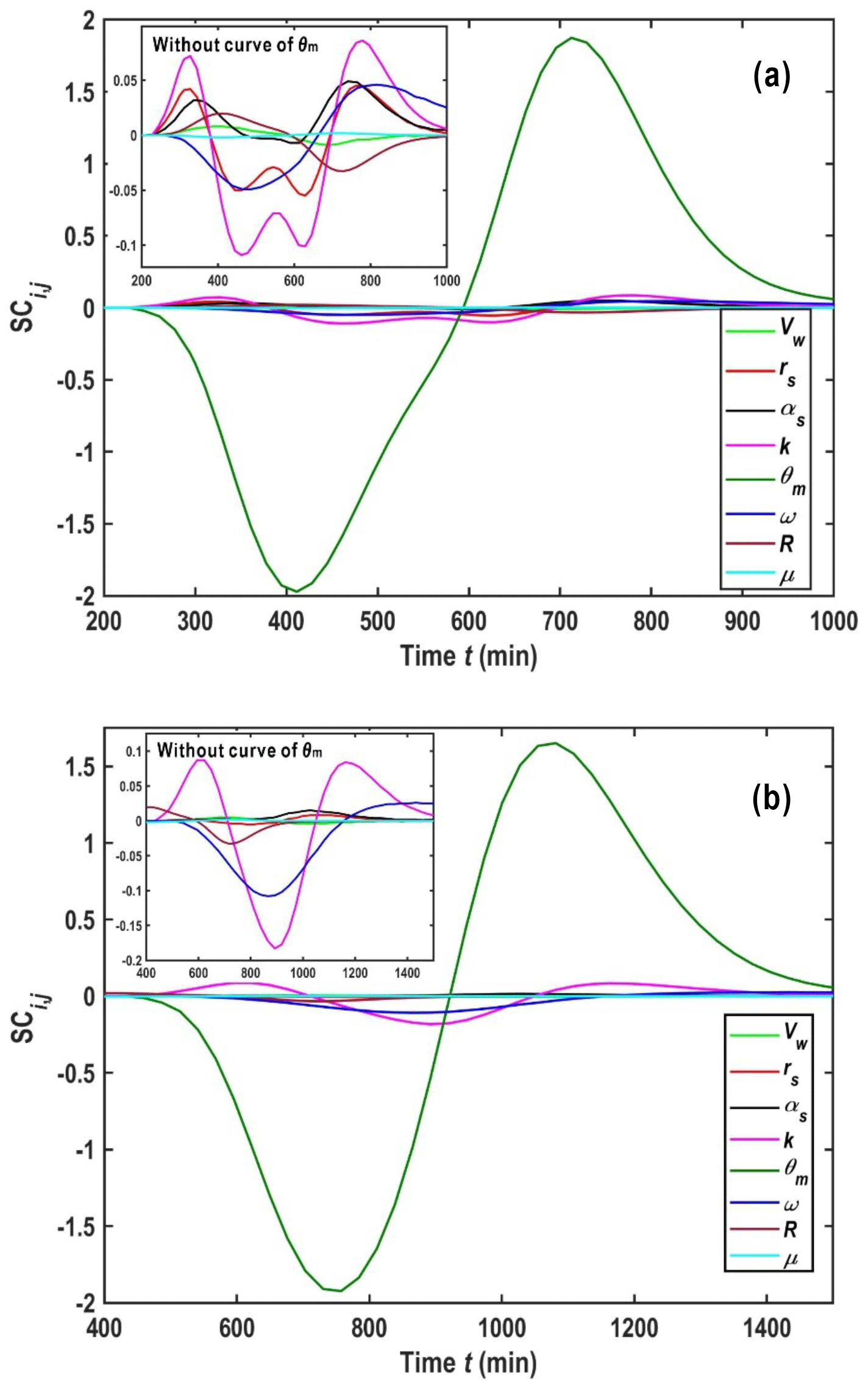
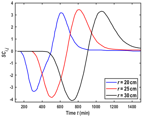
Figure 4SCi,j of the parameters rw, rs, k, θm, ω, R, and μ using the parameters estimated by best-fitting the experimental data. (a) r=22.5 cm; (b) r=30.4 cm.
The main parameters of the new model include the volume of the water in the wellbore (Vw) for the mixing effect, rs and αs for the skin zone, θm and ω for the MIM model, and k for scale-dependent dispersivity. Figure 4a and b show SCi,j at r=22.5 and r=30.4 cm, respectively. The parameters used in these two figures are the same as those used in Fig. 3.
Two observations can be found from Fig. 4a and b. Firstly, the results are sensitive to the parameter of θm. To test such a finding, we use the model of this study (Eqs. 17 and 18) with the mixing effect to best fit the experimental data of Chao (1999) (shown in Fig. S5 in Sect. S5), and the results show that the influence of the mixing effect could be negligible. Secondly, by comparing Fig. 4a and b, we find that the sensitivity coefficient of Vw, rs, αs, and R on BTCs increases with the distance from the wellbore.
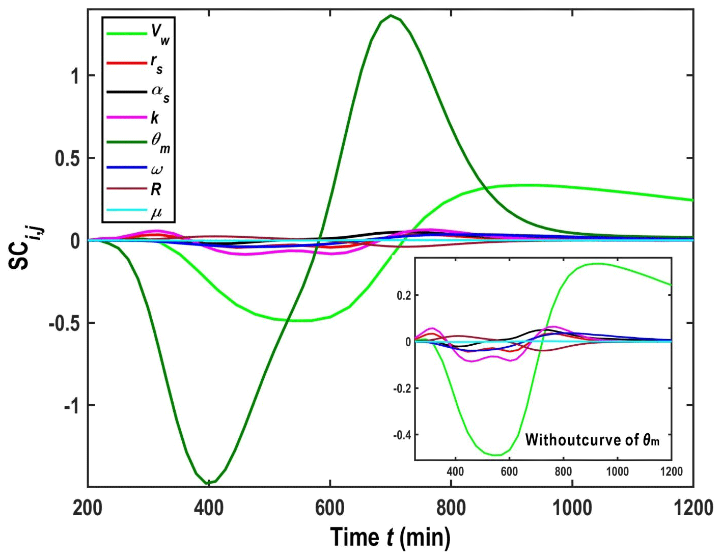
Figure 4a and b show that the sensitivity coefficient of Vw on BTCs is minimal, which might contradict the finding reported in some previous studies (Wang et al., 2018). A careful inspection indicates that the well radius and the initial water level in the wellbore are tiny in the experiment of Chao (1999), resulting in a minimal value of Vw. From Eqs. (6) and (7), one can see that Vw could be influenced by the pumping rate, well radius, initial water level (h0), and hydraulic parameters of the aquifer. In actual field practices, the value of Vw can be significantly larger than what Chao (1999) uses. Therefore, the sensitivity coefficient of Vw on BTCs will be investigated again using the well radius and the initial water level that is more commonly seen in field applications, e.g., rw=5.0 cm and h0=31.75 cm, and the other parameters are the same as the ones in Fig. 3.
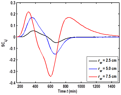
The sensitivity analysis after such modification shows that the parameter with the highest sensitivity coefficient is still θm. However, the parameter with the second-highest sensitivity coefficient becomes the volume of water in the wellbore (Fig. 5). Figures 6 and 7 illustrate SCi,j of Vw for different rw and different observation locations and that the sensitivity coefficient of Vw increases with the well radius but decreases with the distance from the wellbore.
Radial dispersion is an important process in the fields of chemical engineering, environmental science, and hydrogeology. It has been commonly employed to describe the reactive transport in the subsurface or to estimate aquifer transport parameters (dispersivity, porosity, reactive rate, etc.) required in optimization of remediation strategies. However, previous studies did not include all of the mixing effect, skin effect, and mass transfer between the mobile and immobile domains in porous media.
In this study, a new general model is developed considering all the abovementioned factors. The new general model is compared against a finite-element numerical model and existing experimental data. Meanwhile, the new model is also expanded considering the effect of the overlying and underlying aquitards and the scale-dependent dispersivity. The sensitivity analysis is conducted to prioritize influences of various controlling parameters on BTCs. The following conclusions could be summarized.
-
The new general model honors the most relevant processes involved in radial dispersion (wellbore mixing effect, well skin effect, aquitard effect, and mass transfer between the mobile and immobile domains), for which a solution has not yet been presented.
-
The new general model fits the experimental data of Chao (1999) much better than previous models.
-
The results are sensitive to parameters θm (mobile porosity) and Vw (the volume of water in the wellbore). When Vw is very small, as in the laboratory experiment of Chao (1999), the sensitivity coefficient approaches 0. However, for typical values of Vw in actual field applications, the sensitivity coefficient of Vw increases significantly, and the value is often ranked as the second highest, after that of θm.
-
The sensitivity coefficient of Vw increases with well radius, while it decreases with increasing distance from the wellbore.
| Symbol | Description |
| Ai(⋅), Bi(⋅) | Airy functions of the first kind and |
| second kind, respectively | |
| , | Derivative of the Airy functions of the |
| first kind and second kind, respectively | |
| α0 | Longitudinal dispersivity (L) in the |
| formation zone at r>r0 | |
| α1, α2 | Longitudinal dispersivities (L) in the skin |
| and formation zones, respectively | |
| B | The thickness (L) of the aquifer |
| b | Half of the aquifer thickness (L) |
| , | Resident mobile and immobile |
| concentrations (M L−3) of | |
| the skin zone, respectively | |
| , | Resident mobile and immobile |
| concentrations (M L−3) of the formation | |
| zone, respectively | |
| Cum, Cuim | Resident mobile and immobile |
| concentrations (M L−3) of the upper | |
| aquitard, respectively | |
| Clm, Clim | Resident mobile and immobile |
| concentrations (M L−3) of the lower | |
| aquitard, respectively | |
| Cinj(t), Ccha(t) | Concentrations (M L−3) of the tracer |
| in the wellbore in the injection and | |
| chasing phases, respectively | |
| C0 | Concentration (M L−3) of the tracer |
| injected into the wellbore | |
| Cw | Concentration (M L−3) of the tracer |
| in the wellbore | |
| Du, Dl | Vertical dispersion coefficients |
| (L2 T−1) of the upper and | |
| lower aquitards, respectively | |
| D0 | Molecular diffusion coefficient |
| (L2 T−1) | |
| h | Hydraulic head (L) |
| h0 | Hydraulic head (L) at re |
| hw,inj, hw,cha | Water level in the wellbore in the |
| injection and chasing phases (L) | |
| k | A constant (dimensionless) |
| ranging from 0 to 1 | |
| K1, K2 | Hydraulic conductivities (L T−1) of |
| the skin and formation zones, | |
| respectively | |
| Kd | Equilibrium distribution coefficient |
| (M−1 L3) for the linear sorption | |
| process | |
| Im(⋅), Km(⋅) | The mth-order modified Bessel |
| function of the first and second kinds, | |
| respectively | |
| Q | Pumping rate (L3 T−1) (negative for |
| injection and positive for pumping) | |
| Qinj, Qcha | Well flow rates (L3 T−1) in the |
| injection and chasing phases, | |
| respectively. | |
| r | Radial distance (L) from the center |
| of the well | |
| rs | Distance (L) from the center of the |
| well to the outer boundary of the | |
| skin zone | |
| rw | Radius (L) of the well |
| re | Radial distance (L) from the center of |
| the well to the outer boundary | |
| r0 | Radial distance (L) for the linear |
| distance-dependent dispersivity | |
| , | Retardation factors (dimensionless) |
| for the mobile and immobile regions | |
| of the skin zone | |
| , | Retardation factors (dimensionless) |
| for the mobile and immobile regions | |
| of the formation zone | |
| Rum, Ruim | Retardation factors (dimensionless) |
| for the mobile and immobile regions | |
| of the upper aquitard | |
| Rlm, Rlim | Retardation factors (dimensionless) |
| for the mobile and immobile regions | |
| of the lower aquitard | |
| t | Time (T) |
| tinj, tcha | Ending times (T) of the injection and |
| chasing phases, respectively | |
| , | Average radial pore velocities (L T−1) |
| of the skin zone and formation zone, | |
| respectively | |
| , | Average radial pore velocities (L T−1) |
| at the well screen in the injection | |
| and chasing phases, respectively. | |
| vum, vlm | Vertical velocities (L T−1) of the upper |
| and lower aquitards, respectively | |
| αu, αl | Dispersivities (L) of the upper |
| and lower aquitards, respectively | |
| , | Decay constant for radioactive decay |
| or reaction rate coefficient (T−1) in the | |
| mobile and immobile regions of the skin | |
| zone | |
| , | Decay constant (T−1) for radioactive |
| decay or reaction rate coefficient in the | |
| mobile and immobile regions of the | |
| formation zone | |
| μum, μuim | Decay constant (T−1) for radioactive |
| decay or reaction rate coefficient in the | |
| mobile and immobile regions of the | |
| upper aquitard | |
| μlm, μlim | Decay constant (T−1) for radioactive |
| decay or reaction rate coefficient in the | |
| mobile and immobile regions of the | |
| lower aquitard | |
| , | Mobile and immobile porosities |
| (dimensionless) in the skin zone | |
| , | Mobile and immobile porosities |
| (dimensionless) in the formation zone | |
| θum, θuim | Mobile and immobile porosities |
| (dimensionless) in the upper aquitard | |
| θlm, θlim | Mobile and immobile porosities |
| (dimensionless) in the lower aquitard | |
| ρb | Bulk density (M L−3) of the aquifer |
| material | |
| ω1, ω2 | First-order mass transfer coefficients |
| (T−1) in the skin and formation zones, | |
| respectively |
| s | Laplace transform variable with |
| respect to the time tD | |
| Subscript | Description |
| D | Dimensionless form |
| m, im | Mobile and immobile regions, |
| respectively | |
| inj, cha | Injection and chasing phases, |
| respectively | |
| u, l | Upper and lower aquitard, |
| respectively | |
| 1, 2 | Parameters in the skin and |
| formation regions, | |
| respectively | |
| Abbreviation | Description |
| ADE | Advection–dispersion equation |
| BTCs | The observed breakthrough curves |
| CDM | The constant dispersivity model |
| CTRW | Continuous-time random-walk models |
| fADE | Fractional-derivative ADE models |
| GA | The genetic algorithm |
| MFC | The mass flux continuity |
| MIM | Mobile–immobile model |
| MRMT | The multirate mass transfer model |
| RCC | The resident concentration continuity |
| SDM | The scale-dependent dispersivity model |
The code/datasets used and/or analyzed during the current study are available from the corresponding author upon reasonable request.
The supplement related to this article is available online at: https://doi.org/10.5194/hess-27-1891-2023-supplement.
Methodology, derivation, code, formal analysis, writing of original draft: WS. Conceptualization, writing of original draft, writing – review and editing, supervision: QW. Vetting and technical support: HZ, RZ, and YH.
The contact author has declared that none of the authors has any competing interests.
Publisher's note: Copernicus Publications remains neutral with regard to jurisdictional claims in published maps and institutional affiliations.
We thank the editor, associate editor, and two anonymous reviewers for their constructive comments, which helped improve the quality of the paper. We also thank Mohamed Hussein and James J. S. Yeanay Jr. for their help in improving our English.
This research was partially supported by the National Key Research and Development Program of China (grant no. 2021YFA0715900), the National Natural Science Foundation of China (grant nos. 42222704 and 41972250), the Natural Science Foundation of Hubei Province (grant no. 2021CFA089), the Fundamental Research Funds for Central Universities, China University of Geosciences (Wuhan) (grant no. CUGGC07), the 111 Program (State Administration of Foreign Experts Affairs & the Ministry of Education of China, grant no. B18049), the Belt and Road Special Foundation of the State Key Laboratory of Hydrology-Water Resources and Hydraulic Engineering (grant no. 2020492011), and the Natural Science Foundation of Chongqing (grant no. cstc2020jcyj-msxmX1072).
This paper was edited by Alberto Guadagnini and reviewed by two anonymous referees.
Berkowitz, B., Scher, H., and Silliman, S. E.: Anomalous transport in laboratory-scale, heterogeneous porous media, Water Resour. Res., 36, 149–158, https://doi.org/10.1029/1999wr900295, 2000.
Chao, H. C.: Scale dependence of transport parameters estimated from force-gradient tracer tests in heterogeneous formations, PhD thesis, University of Colorado, Boulder, https://www.proquest.com/openview/386f86d718fc9544b2637ce142bc7df5/1?pq-origsite=gscholar&cbl=18750&diss=y (last access: 11 May 2023), 1999.
Chen, C. S.: Analytical and approximate solutions to radial dispersion from an injection well to a geological unit with simultaneous diffusion into adjacent strata, Water Resour. Res., 21, 1069–1076, https://doi.org/10.1029/WR021i008p01069, 1985.
Chen, C. S.: Solutions for radionuclide transport from an injection well into a single fracture in a porous formation, Water Resour. Res., 22, 508–518, https://doi.org/10.1029/WR022i004p00508, 1986.
Chen, C. S.: Semianalytical solutions for radial dispersion in a three-layer leaky aquifer system, Groundwater, 29, 663–670, https://doi.org/10.1111/j.1745-6584.1991.tb00557.x, 1991.
Chen, J.-S., Chen, C.-S., and Chen, C. Y.: Analysis of solute transport in a divergent flow tracer test with scale-dependent dispersion, Hydrol. Process., 21, 2526–2536, https://doi.org/10.1002/hyp.6496, 2007.
Chen, J. S., Liu, Y. H., Liang, C. P., Liu, C. W., and Lin, C. W.: Exact analytical solutions for two-dimensional advection–dispersion equation in cylindrical coordinates subject to third-type inlet boundary condition, Adv. Water Resour., 34, 365–374, https://doi.org/10.1016/j.advwatres.2010.12.008, 2011.
Chen, K., Zhan, H., and Yang, Q.: Fractional models simulating Non-Fickian behavior in four-stage single-well push-pull tests, Water Resour. Res., 53, 9528–9545, https://doi.org/10.1002/2017WR021411, 2017.
Chen, K., Zhan, H., and Zhou, R.: Subsurface solute transport with one-, two-, and three-dimensional arbitrary shape sources, J. Contam. Hydrol., 190, 44–57, https://doi.org/10.1016/j.jconhyd.2016.04.004, 2016.
Chen, Y. J., Yeh, H. D., and Chang, K. J.: A mathematical solution and analysis of contaminant transport in a radial two-zone confined aquifer, J. Contam. Hydrol., 138–139, 75–82, https://doi.org/10.1016/j.jconhyd.2012.06.006, 2012.
Cihan, A. and Tyner, J. S.: 2-D radial analytical solutions for solute transport in a dual-porosity medium, Water Resour. Res., 47, W04507, https://doi.org/10.1029/2009wr008969, 2011.
Dagan, G.: Time-dependent macrodispersion for solute transport in anisotropic heterogeneous aquifers, Water Resour. Res., 24, 1491–1500, https://doi.org/10.1029/WR024i009p01491, 1988.
Davis, M. E. and Davis, R. J.: Fundamentals of chemical reaction engineering, Dover Publications, Inc., New York, NY, USA, https://books.google.fr/books?hl=zh-CN&lr=&id=pAI_YlbVqWQC&oi=fnd&pg=PP1&dq=Fundamentals+of+Chemical+Reaction+Engineering&ots=AtHdptK-wL&sig=-m7CAORXcgN-fFpKzGp4GYSTGuI&redir_esc=y#v=onepage&q=Fundamentals of Chemical Reaction Engineering&f=false (last access: 11 May 2023), 2002.
Deb, K., Agrawal, S., Pratap, A., and Meyarivan, T.: A fast and elitist multiobjective genetic algorithm: NSGA-II, IEEE T. Evol. Comput., 6, 182–197, https://doi.org/10.1109/4235.996017, 2002.
De Hoog, F. R., Knight, J., and Stokes, A.: An improved method for numerical inversion of Laplace transforms, SIAM J. Scient. Stat. Comput., 3, 357–366, https://doi.org/10.1137/0903022, 1982.
Dentz, M., Kang, P. K., and Borgne, T. l.: Continuous time random walks for non-local radial solute transport, Adv. Water Resour., 82, 16–26, https://doi.org/10.1016/j.advwatres.2015.04.005, 2015.
Di Dato, M., Fiori, A., de Barros, F. P., and Bellin, A.: Radial solute transport in highly heterogeneous aquifers: Modeling and experimental comparison, Water Resour. Res., 53, 5725–5741, https://doi.org/10.1002/2016WR020039, 2017.
Dubner, H. and Abate, J.: Numerical Inversion of Laplace Transforms by Relating Them to the Finite Fourier Cosine Transform, J. ACM, 15, 115–123, https://doi.org/10.1145/321439.321446, 1968.
Edery, Y., Dror, I., Scher, H., and Berkowitz, B.: Anomalous reactive transport in porous media: Experiments and modeling, Phys. Rev. E, 91, 052130, https://doi.org/10.1103/PhysRevE.91.052130, 2015.
Elenius, M. T. and Abriola, L. M.: Regressed models for multirate mass transfer in heterogeneous media, Water Resour. Res., 55, 8646–8665, https://doi.org/10.1029/2019wr025476, 2019.
Falade, G. and Brigham, W.: Analysis of radial transport of reactive tracer in porous media, SPE Reserv. Eng., 4, 85–90, https://doi.org/10.2118/16033-PA, 1989.
Freeze, R. A. and Cherry, J. A.: Groundwater, Prentice-Hall, Englewood Cliffs, New Jersey, 604 pp., https://archive.org/details/groundwater-freeze-and-cherry-1979/page/32/mode/2up (last access: 11 May 2023), 1979.
Gao, G., Zhan, H., Feng, S., Fu, B., Ma, Y., and Huang, G.: A new mobile-immobile model for reactive solute transport with scale-dependent dispersion, Water Resour. Res., 46, W08533, https://doi.org/10.1029/2009WR008707, 2010.
Gao, G. Y., Feng, S. Y., Huo, Z. L., Zhan, H. B., and Huang, G. H.: Semi-analytical solution for solute radial transport dynamic model with scale-dependent dispersion, Chinese J. Hydrodynam., 24, 156–163, 2009a.
Gao, G. Y., Feng, S. Y., Zhan, H. B., Huang, G. H., and Mao, X. M.: Evaluation of anomalous solute transport in a large heterogeneous soil column with mobile-immobile model, J. Hydrol. Eng., 14, 966–974, https://doi.org/10.1061/(asce)he.1943-5584.0000071, 2009b.
Gelhar, L. W. and Collins, M. A.: General analysis of longitudinal dispersion in nonuniform flow, Water Resour. Res., 7, 1511–1521, https://doi.org/10.1029/WR007i006p01511, 1971.
Gelhar, L. W., Welty, C., and Rehfeldt, K. R.: A critical review of data on field-scale dispersion in aquifers, Water Resour. Res., 28, 1955–1974, https://doi.org/10.1029/92wr00607, 1992.
Griffioen, J. W., Barry, D. A., and Parlange, J. Y.: Interpretation of two-region model parameters, Water Resour. Res., 34, 373–384, https://doi.org/10.1029/97wr02027, 1998.
Guo, Z., Fogg, G. E., and Henri, C. V.: Upscaling of regional scale transport under transient conditions: Evaluation of the multirate mass transfer model, Water Resour. Res., 55, 5301–5320, https://doi.org/10.1029/2019WR024953, 2019.
Guo, Z., Henri, C. V., Fogg, G. E., Zhang, Y., and Zheng, C.: Adaptive multirate mass transfer (aMMT) model: A new approach to upscale regional-scale transport under transient flow conditions, Water Resour. Res., 56, e2019WR026000, https://doi.org/10.1029/2019WR026000, 2020.
Haddad, A. S., Hassanzadeh, H., Abedi, J., Chen, Z. X., and Ware, A.: Characterization of scale-dependent dispersivity in fractured formations through a divergent flow tracer test, Groundwater, 53, 149–155, https://doi.org/10.1111/gwat.12187, 2015.
Haggerty, R., Fleming, S. W., Meigs, L. C., and McKenna, S. A.: Tracer tests in a fractured dolomite: 2. Analysis of mass transfer in single-well injection-withdrawal tests, Water Resour. Res., 37, 1129–1142, https://doi.org/10.1029/2000WR900334, 2001.
Hansen, S. K., Berkowitz, B., Vesselinov, V. V., O'Malley, D., and Karra, S.: Push-pull tracer tests: Their information content and use for characterizing non-Fickian, mobile-immobile behavior, Water Resour. Res., 52, 9565–9585, https://doi.org/10.1002/2016WR018769, 2016.
Hollenbeck, I.: invlap. m: A matlab function for numerical inversion of Laplace transforms by the de Hoog algorithm, ACM Trans. Math. Softw., 26, 272–278, https://cir.nii.ac.jp/crid/1571135650690787968 (last access: 11 May 2023), 1998.
Hoopes, J. A. and Harleman, D. R.: Dispersion in radial flow from a recharge well, J. Geophys. Res., 72, 3595–3607, https://doi.org/10.1029/JZ072i014p03595, 1967.
Hsieh, P. A.: A new formula for the analytical solution of the radial dispersion problem, Water Resour. Res., 22, 1597–1605, https://doi.org/10.1029/WR022i011p01597, 1986.
Hsieh, P. F. and Yeh, H. D.: Semi-analytical and approximate solutions for contaminant transport from an injection well in a two-zone confined aquifer system, J. Hydrol., 519, 1171–1176, https://doi.org/10.1016/j.jhydrol.2014.08.046, 2014.
Huang, C. S., Tong, C., Hu, W., Yeh, H. D., and Yang, T.: Analysis of radially convergent tracer test in a two-zone confined aquifer with vertical dispersion effect: Asymmetrical and symmetrical transports, J. Hazard. Mater., 377, 8–16, https://doi.org/10.1016/j.jhazmat.2019.05.042, 2019.
Huang, J. and Goltz, M. N.: Analytical solutions for solute transport in a spherically symmetric divergent flow field, Transp. Porous Media, 63, 305–321, https://doi.org/10.1007/s11242-005-6761-4, 2006.
Kabala, Z. J.: Sensitivity analysis of a pumping test on a well with wellbore storage and skin, Adv. Water Resour., 24, 483–504, https://doi.org/10.1016/s0309-1708(00)00051-8, 2001.
Kang, P. K., Le Borgne, T., Dentz, M., Bour, O., and Juanes, R.: Impact of velocity correlation and distribution on transport in fractured media: Field evidence and theoretical model, Water Resour. Res., 51, 940–959, https://doi.org/10.1002/2014WR015799, 2015.
Katoch, S., Chauhan, S. S., and Kumar, V.: A review on genetic algorithm: past, present, and future, Multimed. Tool. Appl., 80, 8091–8126, https://doi.org/10.1007/s11042-020-10139-6, 2020.
Le Borgne, T. and Gouze, P.: Non-Fickian dispersion in porous media: 2. Model validation from measurements at different scales, Water Resour. Res., 44, W06427, https://doi.org/10.1029/2007WR006279, 2008.
Leitão, T. E., Lobo-ferreira, J. P., and Valocchi, A. J.: Application of a reactive transport model for interpreting non-conservative tracer experiments: The Rio Maior case-study, J. Contam. Hydrol., 24, 167–181, https://doi.org/10.1016/S0169-7722(96)00008-3, 1996.
Li, X. T., Wen, Z., Zhan, H., Zhan, H., and Zhu, Q.: Skin effect on single-well push-pull tests with the presence of regional groundwater flow, J. Hydrol., 577, 123931, https://doi.org/10.1016/j.jhydrol.2019.123931, 2019.
Li, X. T., Wen, Z., Zhu, Q., and Jakada, H.: A mobile-immobile model for reactive solute transport in a radial two-zone confined aquifer, J. Hydrol., 580, 124347, https://doi.org/10.1016/j.jhydrol.2019.124347, 2020.
Lu, B., Zhang, Y., Zheng, C., Green, C. T., O'Neill, C., Sun, H.-G., and Qian, J.: Comparison of time nonlocal transport models for characterizing non-Fickian transport: From mathematical interpretation to laboratory application, Water, 10, 778, https://doi.org/10.3390/w10060778, 2018.
Moench, A. and Ogata, A.: A numerical inversion of the Laplace transform solution to radial dispersion in a porous medium, Water Resour. Res., 17, 250–252, https://doi.org/10.1029/WR017i001p00250, 1981.
Molinari, A., Pedretti, D., and Fallico, C.: Analysis of convergent flow tracer tests in a heterogeneous sandy box with connected gravel channels, Water Resour. Res., 51, 5640–5657, https://doi.org/10.1002/2014WR016216, 2015.
Neuman, S. P. and Mishra, P. K.: Comments on “A revisit of drawdown behavior during pumping in unconfined aquifers” by D. Mao, L. Wan, T.-C. J. Yeh, C.-H. Lee, K.-C. Hsu, J.-C. Wen, and W. Lu, Water Resour. Res., 48, W02801, https://doi.org/10.1029/2011wr010785, 2012.
Novakowski, K. S.: The analysis of tracer experiments conducted in divergent radial flow fields, Water Resour. Res., 28, 3215–3225, https://doi.org/10.1029/92WR01722, 1992.
Philip, J.: Some exact solutions of convection-diffusion and diffusion equations, Water Resour. Res., 30, 3545–3551, https://doi.org/10.1029/94WR01329, 1994.
Pickens, J. F. and Grisak, G. E.: Scale-dependent dispersion in a stratified granular aquifer, Water Resour. Res., 17, 1191–1211, https://doi.org/10.1029/WR017i004p01191, 1981a.
Pickens, J. F. and Grisak, G. E.: Modeling of scale-dependent dispersion in hydrogeologic systems, Water Resour. Res., 17, 1701–1711, https://doi.org/10.1029/WR017i006p01701, 1981b.
Reinhard, M., Shang, S., Kitanidis, P. K., Orwin, E., Hopkins, G. D., and Lebrón, C. A.: In Situ BTEX Biotransformation under Enhanced Nitrate- and Sulfate-Reducing Conditions, Environ. Sci. Technol., 31, 28–36, https://doi.org/10.1021/es9509238, 1997.
Schapery, R. A.: Approximate Methods of Transform Inversion for Viscoelastic Stress Analysis, in: Proc. of 4th US National Congress of Applied Mechanics, American Society of Mechanical Engineers, New York, NY, 1075–1085, https://cir.nii.ac.jp/crid/1571135650285612416 (last access: 11 May 2023), 1962.
Shi, W., Wang, Q., and Zhan, H.: New simplified models of single-well push-pull tests with mixing effect, Water Resour. Res., 56, e2019WR026802, https://doi.org/10.1029/2019WR026802, 2020.
Silliman, S. E. and Simpson, E. S.: Laboratory evidence of the scale effect in dispersion of solutes in porous media, Water Resour. Res., 23, 1667–1673, https://doi.org/10.1029/WR023i008p01667, 1987.
Soltanpour Moghadam, A., Arabameri, M., and Barfeie, M.: Numerical solution of space-time variable fractional order advection-dispersion equation using radial basis functions, J. Math. Model., 10, 549–562, https://doi.org/10.22124/JMM.2022.21325.1868, 2022.
Stehfest, H.: Remark on algorithm 368: Numerical inversion of Laplace transforms, Commun. ACM, 13, 617–624, https://doi.org/10.1145/355598.362787, 1970.
Tang, D. and Babu, D.: Analytical solution of a velocity dependent dispersion problem, Water Resour. Res., 15, 1471–1478, https://doi.org/10.1029/WR015i006p01471, 1979.
Tang, D. and Peaceman, D.: New analytical and numerical solutions for the radial convection-dispersion problem, SPE Reserv. Eng., 2, 343–359, https://doi.org/10.2118/16001-PA, 1987.
van Genuchten, M. T. and Wierenga, P. J.: Mass transfer studies in sorbing porous media I. analytical solutions1, Soil Sci. Soc. Am. J., 40, 473–480, https://doi.org/10.2136/sssaj1976.03615995004000040011x, 1976.
Veling, E.: Analytical solution and numerical evaluation of the radial symmetric convection-diffusion equation with arbitrary initial and boundary data, in: Impact of Human Activity on Groundwater Dynamics, edited by: Gehrels, H., Peters, N. E., Hoehn, E., Jensen, K., Leibundgut, C., and Grif, J., IAHS Publ. 269, 271–276, https://www.cabdirect.org/cabdirect/abstract/20013152545 (last access: 11 May 2023), 2001.
Veling, E. J. M.: Radial transport in a porous medium with Dirichlet, Neumann and Robin-type inhomogeneous boundary values and general initial data: analytical solution and evaluation, J. Eng. Math., 75, 173–189, https://doi.org/10.1007/s10665-011-9509-x, 2011.
Wang, Q. and Zhan, H.: Radial reactive solute transport in an aquifer–aquitard system, Adv. Water Resour., 61, 51–61, https://doi.org/10.1016/j.advwatres.2013.08.013, 2013.
Wang, Q. and Zhan, H.: On different numerical inverse Laplace methods for solute transport problems, Adv. Water Resour., 75, 80–92, https://doi.org/10.1016/j.advwatres.2014.11.001, 2015.
Wang, Q., Shi, W., Zhan, H., Gu, H., and Chen, K.: Models of single-well push-pull test with mixing effect in the wellbore, Water Resour. Res., 54, 10155–10171, https://doi.org/10.1029/2018wr023317, 2018.
Wang, Q., Gu, H., Zhan, H., Shi, W., and Zhou, R.: Mixing effect on reactive transport in a column with scale dependent dispersion, J. Hydrol., 582, 124494, https://doi.org/10.1016/j.jhydrol.2019.124494, 2019.
Wang, Q., Wang, J., Zhan, H., and Shi, W.: New model of reactive transport in a single-well push–pull test with aquitard effect and wellbore storage, Hydrol. Earth Syst. Sci., 24, 3983–4000, https://doi.org/10.5194/hess-24-3983-2020, 2020.
Webster, D. S., Procter, J. F., and Marine, J. W.: Two-well tracer test in fractured crystalline rock, Water Supply Paper 1544-1574, US Geological Survey, https://doi.org/10.3133/wsp1544I, 1970.
Whitley, L. D.: A genetic algorithm tutorial, Stat. Comput., 4, 65–85, https://doi.org/10.1007/BF00175354, 1994.
Yang, S.-Y. and Yeh, H.-D.: Radial groundwater flow to a finite diameter well in a leaky confined aquifer with a finite-thickness skin, Hydrol. Process., 23, 3382–3390, https://doi.org/10.1002/hyp.7449, 2009.
Yates, S.: Three-dimensional radial dispersion in a variable velocity flow field, Water Resour. Res., 24, 1083–1090, https://doi.org/10.1029/WR024i007p01083, 1988.
Yeh, H. D. and Chang, Y. C. i.: Recent advances in modeling of well hydraulics, Adv. Water Resour., 51, 27–51, https://doi.org/10.1016/j.advwatres.2012.03.006, 2013.
Zakian, V.: Numerical inversion of Laplace transform, Electron. Lett., 5, 120–121, 1969.
Zhan, H. B., Wen, Z., and Gao, G. Y.: An analytical solution two-dimensional reactive solute transport in an aquifer–aquitard system, Water Resour. Res., 45, W10501, https://doi.org/10.1029/2008WR007479, 2009a.
Zhan, H. B., Wen, Z., Huang, G. H., and Sun, D. M.: Analytical solution of two-dimensional solute transport in an aquifer–aquitard system, J. Contam. Hydrol., 107, 162–174, https://doi.org/10.1016/j.jconhyd.2009.04.010, 2009b.
Zheng, C. and Wang, P. P.: MT3DMS: a modular three-dimensional multispecies transport model for simulation of advection, dispersion, and chemical reactions of contaminants in groundwater systems; documentation and user's guide, Alabama University, http://hdl.handle.net/11681/4734 (last access: 11 May 2023), 1999.
Zheng, L., Wang, L., and James, S. C.: When can the local advection–dispersion equation simulate non-Fickian transport through rough fractures?, Stoch. Environ. Res. Risk A., 33, 931–938, https://doi.org/10.1007/s00477-019-01661-7, 2019.
Zhou, R., Zhan, H., and Chen, K.: Reactive solute transport in a filled single fracture-matrix system under unilateral and radial flows, Adv. Water Resour., 104, 183–194, https://doi.org/10.1016/j.advwatres.2017.03.022, 2017.