A signal-processing-based interpretation of the Nash–Sutcliffe efficiency

The Nash–Sutcliffe efficiency (NSE) is a widely used score in hydrology, but it is not common in the other environmental sciences. One of the reasons for its unpopularity is that its scientific meaning is somehow unclear in the literature. This study attempts to establish a solid foundation for the NSE from the viewpoint of signal progressing. Thus, a simulation is viewed as a received signal containing a wanted signal (observations) contaminated by an unwanted signal (noise). This view underlines an important role of the error model between simulations and observations.

By assuming an additive error model, it is easy to point out that the NSE is equivalent to an important quantity in signal processing: the signal-to-noise ratio. Moreover, the NSE and the Kling–Gupta efficiency (KGE) are shown to be equivalent, at least when there are no biases, in the sense that they measure the relative magnitude of the power of noise to the power of the variation in observations. The scientific meaning of the NSE suggests a natural way to define NSE=0 as the threshold for good or bad model distinction, and this has no relation to the benchmark simulation that is equal to the observed mean. Corresponding to NSE=0, the threshold of the KGE is given by approximately 0.5.

In the general cases, when the additive error model is replaced by a mixed additive–multiplicative error model, the traditional NSE is shown to be prone to contradiction in model evaluations. Therefore, an extension of the NSE is derived, which only requires one to divide the traditional noise-to-signal ratio by the multiplicative bias. This has a practical implication: if the multiplicative bias is not considered, the traditional NSE and KGE underestimate or overestimate the generalized NSE and KGE when the multiplicative bias is greater or smaller than one, respectively. In particular, the observed mean turns out to be the worst simulation from the viewpoint of the generalized NSE.

1 Introduction

In hydrology, the Nash–Sutcliffe efficiency (NSE) is one of the most widely used similarity measures for calibration, model comparison, and verification (ASCE, 1993; Legates and McCabe, 1999; Moriasi et al., 2007; Pushpalatha et al., 2012; Todini and Biondi, 2017). However, Schaefli and Gupta (2007) pointed out the noticeable fact that the NSE is not commonly used in other environmental science fields, despite the fact that calibration, model comparison, and verification are also employed in such fields. Does this mean that the NSE is a special metric that is only relevant for hydrological processes? If this is not the case, what causes this limited use outside of hydrology? One of the reasons for the limited use of the NSE outside of hydrology can be traced back to the lack of a consensual scientific meaning in the literature.

The NSE was first proposed by Nash and Sutcliffe (1970), who approached calibration from a linear regression viewpoint (Murphy et al., 1989).

$$\begin{array}{}\text{(1)}& \text{NSE}=\mathrm{1}-{\displaystyle \frac{\sum (o_i-s_i{)}^{\mathrm{2}}}{\sum (o_i-{\mathit{\mu }}_o{)}^{\mathrm{2}}}}=\mathrm{1}-{\displaystyle \frac{\stackrel{\mathrm{‾}}{(o-s{)}^{\mathrm{2}}}}{\stackrel{\mathrm{‾}}{(o-{\mathit{\mu }}_o{)}^{\mathrm{2}}}}},\end{array}$$

where s_i and o_i denote simulations and observations, respectively; $\stackrel{\mathrm{‾}}{\left(\right)}$ denotes the expectation; and ${\mathit{\mu }}_o=\stackrel{\mathrm{‾}}{o}$ is the observed mean. The authors noted the analogy between the NSE and the coefficient of determination (R²) in linear regression. As R² measures the goodness of fit in linear regression, the NSE should yield a similarity measure for our calibration problem. This use of R² implies that the NSE regresses observations on simulations:

$$\begin{array}{}\text{(2)}& o=as+b,\end{array}$$

where a and b are the linear regression coefficients. Then the residual sum $\sum (o_i-s_i{)}^{\mathrm{2}}$, which they called the residual variance, and the total sum $\sum (o_i-{\mathit{\mu }}_o{)}^{\mathrm{2}}$, which they called the initial variance, are used in the definition of the NSE. In general cases, the residual sum should be $\sum (o_i-a{s}_i-b{)}^{\mathrm{2}}$. This points out that the underlying regression model implicitly assumes an unbiased regression line ($a=\mathrm{1},b=\mathrm{0}$), which is rarely satisfied in reality.

A similar efficiency was introduced in Ding (1974), 4 years after the introduction of the NSE. We call this efficiency the Nash–Ding efficiency (NDE):

$$\begin{array}{}\text{(3)}& \text{NDE}=\mathrm{1}-{\displaystyle \frac{\sum (s_i-o_i{)}^{\mathrm{2}}}{\sum (s_i-{\mathit{\mu }}_o{)}^{\mathrm{2}}}}=\mathrm{1}-{\displaystyle \frac{\stackrel{\mathrm{‾}}{(s-o{)}^{\mathrm{2}}}}{\stackrel{\mathrm{‾}}{(s-{\mathit{\mu }}_o{)}^{\mathrm{2}}}}}.\end{array}$$

Like the NSE, the NDE can also be explained from the viewpoint of linear regression by switching the roles of o and s in Eq. (2) (i.e., by regressing simulations on observations):

$$\begin{array}{}\text{(4)}& s=ao+b.\end{array}$$

Using this regression equation, the coefficient of determination (R²) will take the form shown in Eq. (3) if we again assume an unbiased regression line ($a=\mathrm{1},b=\mathrm{0}$), as in the case of the NSE. Note that, in this case, the total sum is given by $\sum (s_i-\stackrel{\mathrm{‾}}{s}{)}^{\mathrm{2}}$; because of the no bias assumption $\stackrel{\mathrm{‾}}{s}=\stackrel{\mathrm{‾}}{o}$, this becomes $\sum (s_i-{\mathit{\mu }}_o{)}^{\mathrm{2}}$ in Eq. (3). It is interesting to see that the hydrology community have preferred the use of the NSE in calibration, even though the regression of observations on simulations does not show any advantage over the regression of simulations on observations.

Identifying the NSE as R² in linear regression was soon replaced by identifying the NSE as skill scores in verification (ASCE, 1993; Moriasi et al., 2007; Schaefli and Gupta, 2007; Ritter and Munoz-Carpena, 2013). Here, a skill score measures the relative performance between a score and its benchmark or baseline (Murphy, 1988). This benchmark score is obtained by using a benchmark simulation, which is usually an easily accessible simulation that does not require complicated computation. The most common benchmarks are long-term or climatological means. Thus, with respect to the NSE, the numerator $\sum (o_i-f_i{)}^{\mathrm{2}}$ is simply the familiar mean-squared error (MSE) score, and the denominator $\sum (o_i-{\mathit{\mu }}_o{)}^{\mathrm{2}}$ is now reinterpreted as the MSE of the benchmark given by the observed mean f_i=μ_o. Equivalently, the NSE can also be viewed as a normalized MSE with the normalizing factor $\sum (o_i-{\mathit{\mu }}_o{)}^{\mathrm{2}}$ (Moriasi et al., 2007; Lamontagne et al., 2020).

However, when applied to forecast verification, in which simulations are replaced by forecasts, the special choice of μ_o as the benchmark does not conform to the purpose of using skill scores. Here, the problem is that the observed mean can only be accessed after all observations are realized; it is not available at the time that we issue forecasts and, therefore, cannot be compared with our forecasts at that time. This subtle problem has been noticed by several authors (Legates and McCabe, 1999; Seibert, 2001), and seasonal or climatological means have been suggested as benchmarks instead of the observed mean. However, Legates and McCabe (2012) showed that the appropriate choice of benchmark depends on the hydrological regime, leading to a more complicated use of the NSE in verification. Therefore, they suggested sticking with the original NSE.

In recent years, starting with the work of Gupta and Kling (2011), the NSE has been recognized as a compromise between different criteria that measures overall performance by combining different scores for means, variances, and correlations. The decomposed form of the NSE in terms of the correlation ρ, the ratio of standard deviations $\mathit{\alpha }={\mathit{\sigma }}_s/{\mathit{\sigma }}_o$, and the ratio of means $\mathit{\beta }={\mathit{\mu }}_s/{\mathit{\mu }}_o$ is given by

$$\begin{array}{}\text{(5)}& \text{NSE}=\mathrm{2}\mathit{\alpha }\mathit{\rho }-{\mathit{\alpha }}^{\mathrm{2}}-{\displaystyle \frac{(\mathit{\beta }-\mathrm{1}{)}^{\mathrm{2}}}{({\mathit{\sigma }}_o/{\mathit{\mu }}_o{)}^{\mathrm{2}}}}.\end{array}$$

Given this unintuitive form of the NSE, Gupta et al. (2009) suggested a more intuitive score called the Kling–Gupta efficiency (KGE):

$$\begin{array}{}\text{(6)}& \text{KGE}=\mathrm{1}-\sqrt{w_{\mathit{\rho }}(\mathit{\rho }-\mathrm{1}{)}^{\mathrm{2}}+w_{\mathit{\alpha }}(\mathit{\alpha }-\mathrm{1}{)}^{\mathrm{2}}+w_{\mathit{\beta }}(\mathit{\beta }-\mathrm{1}{)}^{\mathrm{2}}},\end{array}$$

where w_ρ,w_α, and w_β are weights for individual scores and are usually set to one. Note that this mathematical form (Eq. 6) is only one of many potential combinations of ρ,α, and β that yield an appropriate verification score. In this multiple-criteria framework, the scientific meaning of the KGE depends on the weights that we assign to individual scores. However, unlike the KGE, the NSE defined by Eq. (5) is not a linear combination of the individual scores related to ρ,α, and β; therefore, the scientific meaning of the NSE is even more obscure in this context. In other words, we can simply explain that the NSE measures overall performance, but we cannot separate the contribution from each individual score.

One of weak points of the multiple-criteria viewpoint is that it explains the elegant form (Eq. 1) using the unintuitive form (Eq. 5). We suspect that a more profound explanation for the elegant form (Eq. 1) exists that also gives us the scientific meaning of the NSE. In pursuing this explanation, we will come back to the insight of Nash and Sutcliffe (1970) when they first proposed the NSE as a measure. This insight was expressed clearly in Moriasi et al. (2007), who understood the NSE as the relative magnitude of the variances in noise and the variances in informative signals. This encouraged us to approach the NSE from the perspective of signal processing. We will show that the NSE is indeed a well-known quantity in signal processing.

This paper is organized as follows. In Sect. 2, we revisit the traditional NSE from the viewpoint of signal processing of simulations and observations. In practice, the nature and behavior of the NSE can only be established with an additive error model imposing on simulations and observations. As the additive error model implies that the variances in simulations are greater than variances in observations, Sect. 3 extends the error model from Sect. 2 by introducing multiplicative biases in addition to additive biases in order to cover other cases. An extension of the NSE in these general cases is then derived. Finally, Sect. 4 summarizes the main findings of this study and discusses some implications of using the NSE in practice.

2 Specific cases: additive error models

2.1 The scientific meaning of the NSE

From now on, we will consider simulations and observations from the perspective of signal processing. According to this view, observations form a desired signal that we wish to faithfully reproduce whenever we run a model to simulate such observations. This simulation introduces another signal known as the received signal in signal processing, and it is assumed to be the wanted signal (the observations) contaminated by a certain unwanted signal (noise). This means that we will have a good simulation whenever model errors, as represented by the noise, are small. In this section, we assume a simple additive error model for simulations:

$$\begin{array}{}\text{(7)}& s=o+b+\mathit{\epsilon },\end{array}$$

where b denotes constant systematic errors and $\mathit{\epsilon }\sim \mathcal{N}(\mathrm{0},{\mathit{\sigma }}_e^{\mathrm{2}})$ denotes random errors with the error variance ${\mathit{\sigma }}_e^{\mathrm{2}}$. The two random variables o and ε are assumed to be uncorrelated.

Using the error model shown in Eq. (7), it is easy to calculate two expectations in the formula of the NSE,

$$\begin{array}{}\text{(8)}& {\displaystyle }\text{MSE}=\stackrel{\mathrm{‾}}{(s-o{)}^{\mathrm{2}}}=b^{\mathrm{2}}+{\mathit{\sigma }}_e^{\mathrm{2}}\text{and}\text{(9)}& {\displaystyle }\stackrel{\mathrm{‾}}{(o-{\mathit{\mu }}_o{)}^{\mathrm{2}}}={\mathit{\sigma }}_o^{\mathrm{2}},\end{array}$$

leading to the following form of the NSE:

$$\begin{array}{}\text{(10)}& \text{NSE}=\mathrm{1}-{\displaystyle \frac{b^{\mathrm{2}}+{\mathit{\sigma }}_e^{\mathrm{2}}}{{\mathit{\sigma }}_o^{\mathrm{2}}}}.\end{array}$$

The reciprocal of the ratio $(b^{\mathrm{2}}+{\mathit{\sigma }}_e^{\mathrm{2}})/{\mathit{\sigma }}_o^{\mathrm{2}}$ in Eq. (10) represents the signal-to-noise ratio (SNR) in signal processing:

$$\begin{array}{}\text{(11)}& \begin{array}{rl}\text{SNR}& ={\displaystyle \frac{P_{\text{signal}}}{P_{\text{noise}}}}={\displaystyle \frac{\stackrel{\mathrm{‾}}{o^{\mathrm{2}}}}{\stackrel{\mathrm{‾}}{(b+\mathit{\epsilon }{)}^{\mathrm{2}}}}}\\ & ={\displaystyle \frac{\stackrel{\mathrm{‾}}{({\mathit{\mu }}_o+o-{\mathit{\mu }}_o{)}^{\mathrm{2}}}}{\stackrel{\mathrm{‾}}{(b+\mathit{\epsilon }{)}^{\mathrm{2}}}}}={\displaystyle \frac{{\mathit{\mu }}_o^{\mathrm{2}}+{\mathit{\sigma }}_o^{\mathrm{2}}}{b^{\mathrm{2}}+{\mathit{\sigma }}_e^{\mathrm{2}}}},\end{array}\end{array}$$

where P_signal and P_noise are the power of the desired signal and noise, respectively. The greater the SNR, the better the received signal.

In order to examine the relationship between the NSE and SNR, we note that the error model shown in Eq. (7) is preserved in the translations $(s,o)\to (s+\mathrm{\Delta },o+\mathrm{\Delta })$, where Δ is an arbitrary real number. This is easy to verify, as the same error model is obtained when we add the same value Δ to s and o on both sides of Eq. (7). A robust score should reflect this invariance and, therefore, is required to be invariant in those translations. If this condition is not satisfied, we will get a different score every time that we change the base in calculating water levels, for example. It is clear that the NSE is translation invariant, whereas the SNR is not. Indeed, we can easily increase the SNR by simply increasing μ_o:

$$\begin{array}{}\text{(12)}& \text{SNR}\left(\mathrm{\Delta }\right)={\displaystyle \frac{({\mathit{\mu }}_o+\mathrm{\Delta }{)}^{\mathrm{2}}+{\mathit{\sigma }}_o^{\mathrm{2}}}{b^{\mathrm{2}}+{\mathit{\sigma }}_e^{\mathrm{2}}}}.\end{array}$$

This is because the magnitude of the desired signal is almost dominated by Δ and the noise magnitude becomes negligible when a large Δ is added to the desired signal. This suggests that we can use the lower bound of the SNR(Δ), i.e., the SNR in the worst case, as a score to impose the translation-invariant condition:

$$\begin{array}{}\text{(13)}& {\text{SNR}}_{\mathrm{l}}={\displaystyle \frac{{\mathit{\sigma }}_o^{\mathrm{2}}}{b^{\mathrm{2}}+{\mathit{\sigma }}_e^{\mathrm{2}}}}.\end{array}$$

This value is attained when $\mathrm{\Delta }=-{\mathit{\mu }}_o$, which indicates the ratio of the power of the variation o−μ_o to the power of noise. It is worth noting that the translational invariance is violated in the case of the KGE, as the ratio $({\mathit{\mu }}_s+\mathrm{\Delta })/({\mathit{\mu }}_o+\mathrm{\Delta })$ can vary considerably with Δ.

Because the reciprocal of SNR_l determines the NSE in Eq. (10), it is more appropriate to define the NSE in terms of the noise-to-signal ratio ($\text{NSR}=P_{\text{noise}}/P_{\text{signal}}$):

$$\begin{array}{}\text{(14)}& \text{NSE}=\mathrm{1}-{\displaystyle \frac{\mathrm{1}}{{\text{SNR}}_{\mathrm{l}}}}=\mathrm{1}-{\text{NSR}}_{\mathrm{u}},\end{array}$$

where we add the subscript “u” to the NSR to emphasize that this is the upper bound of the NSR corresponding to the lower bound of the SNR. Thus, using our additive error model, Eq. (14) points out that the NSE is equivalent to the upper bound of the NSR. More exactly, the NSE measures the relative magnitude of the power of noise (the unwanted signal) and the power of the variation in observations (the wanted signal with its mean removed). Similarly, it is easy to show that the NDE (Eq. 3) is also a simple function of NSR_u:

$$\begin{array}{}\text{(15)}& \begin{array}{rl}\text{NDE}& =\mathrm{1}-{\displaystyle \frac{b^{\mathrm{2}}+{\mathit{\sigma }}_e^{\mathrm{2}}}{{\mathit{\sigma }}_o^{\mathrm{2}}+b^{\mathrm{2}}+{\mathit{\sigma }}_e^{\mathrm{2}}}}={\displaystyle \frac{{\mathit{\sigma }}_o^{\mathrm{2}}}{{\mathit{\sigma }}_o^{\mathrm{2}}+b^{\mathrm{2}}+{\mathit{\sigma }}_e^{\mathrm{2}}}}\\ & ={\displaystyle \frac{\mathrm{1}}{\mathrm{1}+{\text{NSR}}_{\mathrm{u}}}}.\end{array}\end{array}$$

Again, the NSE and NDE are shown to be equivalent, although this time from the perspective of signal processing.

This new interpretation of the NSE has two important implications for the use of the NSE in practice. Firstly, note that the NSR depends not only on the power of noise but also on the power of the signals under consideration. Thus, the NSE should not be used as a performance measure when comparing two different kinds of signals. We may commit a possibly erroneous assessment by considering that our model is better for flow regime A than for flow regime B, when this may be the consequence of the simple fact that the signals in case A are stronger than those in case B. From its mathematical form, it is clear that the NSR favors high-power signals (i.e., strong signals always result in a small NSR); therefore, it is easy to get high NSE values for strong signals. Such NSE values may be wrongly identified as an indicator of good performance, resulting in misleading evaluations of model performance.

Secondly, as a ratio of the power of noise to the power of the variation in observations, the NSR_u suggests a natural way to define an NSE threshold that divides simulations into “good” and “bad” simulations. Note that NSR_u=0 for perfect simulations and increases with increasing power of noise. At NSR_u=1, the noise has the same power as the variation in the desired signal and, consequently, corrupts the desired signal. In other words, we cannot distinguish variation in observations from noise, and the model simulations are therefore useless. Corresponding to NSR_u=1, we have the two thresholds NSE=0 and $\text{NDE}=\mathrm{1}/\mathrm{2}$. In the context of skill scores, an NSE of zero is also chosen as the boundary between good and bad simulations by requiring that good simulations have MSE values smaller than the MSE of the observed mean s=μ_o. Clearly, the two interpretations are very different, even though they give the same benchmark, NSE=0. Whereas the choice of the observed mean as the benchmark simulation is quite arbitrary in the latter interpretation, such a benchmark is not needed in the former interpretation. In fact, many models yielding the value NSE=0 exist that are not necessarily the observed mean. A further argument supporting the former approach is the failure of the latter approach when applied to the case of the NDE. For the benchmark model s=μ_o, the NDE becomes −∞, which means that all other simulations are always better than this benchmark as measured by the NDE.

2.2 Random noise-to-signal ratio

Recall that the NSE is invariant in the translations along the vector $(\mathrm{1},\mathrm{1}{)}^{\mathrm{T}}(f,o)\to (f+\mathrm{\Delta },o+\mathrm{\Delta })$. However, for general translations $(f,o)\to (f+{\mathrm{\Delta }}_f,o+{\mathrm{\Delta }}_o)$, where the translation vector (Δ_f,Δ_o)^T is an arbitrary vector, the NSE can take any value:

$$\begin{array}{}\text{(16)}& \text{NSE}=\mathrm{1}-{\displaystyle \frac{(b+{\mathrm{\Delta }}_f-{\mathrm{\Delta }}_o{)}^{\mathrm{2}}+{\mathit{\sigma }}_e^{\mathrm{2}}}{{\mathit{\sigma }}_o^{\mathrm{2}}}}.\end{array}$$

Consequently, we can increase the NSE simply by choosing an appropriate Δ_f and Δ_o. In practice, this approach is known as bias correction, with the choice of ${\mathrm{\Delta }}_f\approx -b$ and Δ_o=0. As the NSE is not invariant in the general translations, misinterpretation of model performance can be easily committed. For example, let us consider two simulations: one with a systematic error and one with a random error:

$$\begin{array}{}\text{(17a)}& {\displaystyle }{s}_{\mathrm{1}}=o+b,\text{(17b)}& {\displaystyle }{s}_{\mathrm{2}}=o+\mathit{\epsilon }.\end{array}$$

Here, we assume ${\mathit{\sigma }}_o=b={\mathit{\sigma }}_e$. Thus, both s₁ and s₂ have ${\text{NSE}}_{\mathrm{1}}={\text{NSE}}_{\mathrm{2}}=\mathrm{0}$, indicating that both simulations are corrupted by model errors. However, it is clear that two simulations are not equal. From experience, modelers know that the first simulation is better, as an almost perfect simulation can be easily obtained from s₁ just by subtracting the bias estimated from observations from s₁. In contrast, the performance of s₂ cannot be improved by any translation.

In order to avoid the abovementioned misjudgment, it is desirable to have a score that is invariant in any translation. From Eq. (16), it is easy to see that the bias term causes the NSE to vary with different displacements of f and o. This motivates us to decompose NSR_u into two components:

$$\begin{array}{}\text{(18)}& {\text{NSR}}_{\mathrm{u}}={\displaystyle \frac{b^{\mathrm{2}}+{\mathit{\sigma }}_e^{\mathrm{2}}}{{\mathit{\sigma }}_o^{\mathrm{2}}}}={\displaystyle \frac{b^{\mathrm{2}}}{{\mathit{\sigma }}_o^{\mathrm{2}}}}+{\displaystyle \frac{{\mathit{\sigma }}_e^{\mathrm{2}}}{{\mathit{\sigma }}_o^{\mathrm{2}}}}={\text{SNSR}}_{\mathrm{u}}+{\text{RNSR}}_{\mathrm{u}},\end{array}$$

where SNSR_u denotes the systematic NSR_u, which changes with the general translations, and RNSR_u denotes the random NSR_u, which remains constant regardless of translations. Thus, RNSR_u is an irreducible component of NSR_u in any translation and acts as a lower bound of NSR_u. Similar to Eq. (14), we define a generally invariant version of the NSE in terms of RNSR_u:

$$\begin{array}{}\text{(19)}& {\text{NSE}}_{\mathrm{u}}=\mathrm{1}-{\displaystyle \frac{{\mathit{\sigma }}_e^{\mathrm{2}}}{{\mathit{\sigma }}_o^{\mathrm{2}}}}=\mathrm{1}-{\text{RNSR}}_{\mathrm{u}}.\end{array}$$

Here, the subscript “u” is added to emphasize that this NSE is indeed the upper bound of the original NSE (i.e., the highest NSE can be reached just by translations). The NSE_u is identical to the NSE when there are no biases in simulations. For the two simulations s₁ and s₂ in Eqs. (17a) and (17b), respectively, the new score yields NSE_u1=1 and NSE_u2=0, respectively, which reflect our subjective evaluation. As we shall see shortly, RNSR_u will help to ease our analysis on the behavior of the NSE considerably.

Similar to NSE_u, we define NDE_u in terms of RNSR_u:

$$\begin{array}{}\text{(20)}& {\text{NDE}}_{\mathrm{u}}={\displaystyle \frac{\mathrm{1}}{\mathrm{1}+{\text{RNSR}}_{\mathrm{u}}}}.\end{array}$$

We now prove an interesting fact: that NDE_u is indeed a more familiar quantity in statistics, namely the correlation coefficient ρ. This is easy to prove by making use of Eq. (7) in the definition of ρ,

$$\begin{array}{}\text{(21)}& \begin{array}{rl}\mathit{\rho }& ={\displaystyle \frac{\stackrel{\mathrm{‾}}{(s-{\mathit{\mu }}_s)(o-{\mathit{\mu }}_o)}}{{\mathit{\sigma }}_s{\mathit{\sigma }}_o}}={\displaystyle \frac{\stackrel{\mathrm{‾}}{(o-{\mathit{\mu }}_o+\mathit{\epsilon })(o-{\mathit{\mu }}_o)}}{{\mathit{\sigma }}_s{\mathit{\sigma }}_o}}\\ & ={\displaystyle \frac{{\mathit{\sigma }}_o^{\mathrm{2}}}{{\mathit{\sigma }}_s{\mathit{\sigma }}_o}}={\displaystyle \frac{{\mathit{\sigma }}_o}{{\mathit{\sigma }}_s}}>\mathrm{0},\end{array}\end{array}$$

and in the definition of ${\mathit{\sigma }}_f^{\mathrm{2}}$,

$$\begin{array}{}\text{(22)}& {\mathit{\sigma }}_s^{\mathrm{2}}=\stackrel{\mathrm{‾}}{(s-{\mathit{\mu }}_s{)}^{\mathrm{2}}}=\stackrel{\mathrm{‾}}{(o-{\mathit{\mu }}_o+\mathit{\epsilon }{)}^{\mathrm{2}}}={\mathit{\sigma }}_o^{\mathrm{2}}+{\mathit{\sigma }}_e^{\mathrm{2}}.\end{array}$$

By plugging Eq. (22) into Eq. (21), we obtain a one-to-one map between ρ² and RNSR_u:

$$\begin{array}{}\text{(23)}& {\mathit{\rho }}^{\mathrm{2}}={\displaystyle \frac{{\mathit{\sigma }}_o^{\mathrm{2}}}{{\mathit{\sigma }}_s^{\mathrm{2}}}}={\displaystyle \frac{{\mathit{\sigma }}_o^{\mathrm{2}}}{{\mathit{\sigma }}_o^{\mathrm{2}}+{\mathit{\sigma }}_e^{\mathrm{2}}}}={\displaystyle \frac{\mathrm{1}}{\mathrm{1}+{\text{RNSR}}_{\mathrm{u}}}}={\text{NDE}}_{\mathrm{u}}.\end{array}$$

This reveals a profound understanding of ρ, i.e., the correlation reflects noisiness in the error model shown in Eq. (7). This is illustrated in Fig. 1 with the joint probability distributions of s and o for different values of ρ. From Eq. (23), it is easy to find the lowest correlation at which a simulation is still considered to be good:

$$\begin{array}{}\text{(24)}& {\text{NDE}}_{\mathrm{u}}={\mathit{\rho }}^{\mathrm{2}}\ge \text{NDE}\ge {\displaystyle \frac{\mathrm{1}}{\mathrm{2}}}\leftrightarrow \mathit{\rho }\ge {\displaystyle \frac{\mathrm{1}}{\sqrt{\mathrm{2}}}}\approx \mathrm{0.7}.\end{array}$$

It is worth noting that this critical value of ρ is unknown in the literature.

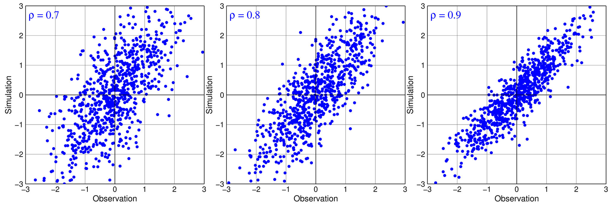
Figure 1 Joint probability distributions of simulations and observations with different values of ρ in the additive error model. Here, we assume b=0 and $o\sim \mathcal{N}(\mathrm{0},\mathrm{1})$; thus, the error model yields ${\mathit{\sigma }}_e=\sqrt{\mathrm{1}/{\mathit{\rho }}^{\mathrm{2}}-\mathrm{1}}{\mathit{\sigma }}_o$.

2.3 Relationships between the NSE, NDE, and KGE

In the previous section, we showed that the four variables NSE_u, NDE_u, ρ, and RNSR_u are equivalent in the sense that they reflect noise levels in simulations. As the correlation (ρ) is a more popular variable, with its support on the finite interval [0,1], we will use ρ as the main independent variable and view all scores as functions of ρ in this section. Thus, the expression of NSE_u in terms of ρ is given by

$$\begin{array}{}\text{(25)}& {\text{NSE}}_{\mathrm{u}}=\mathrm{1}-{\text{RNSR}}_{\mathrm{u}}=\mathrm{2}-{\displaystyle \frac{\mathrm{1}}{{\mathit{\rho }}^{\mathrm{2}}}}.\end{array}$$

Similarly, we disregard the contribution from the means μ_s and μ_o to the KGE in Eq. (6) and define its upper bound by setting all of the weights to 1.0:

$$\begin{array}{}\text{(26)}& \begin{array}{rl}{\text{KGE}}_{\mathrm{u}}& =\mathrm{1}-\sqrt{(\mathit{\rho }-\mathrm{1}{)}^{\mathrm{2}}+{\left({\displaystyle \frac{{\mathit{\sigma }}_s}{{\mathit{\sigma }}_o}}-\mathrm{1}\right)}^{\mathrm{2}}}\\ & =\mathrm{1}-\sqrt{(\mathit{\rho }-\mathrm{1}{)}^{\mathrm{2}}+{\left({\displaystyle \frac{\mathrm{1}}{\mathit{\rho }}}-\mathrm{1}\right)}^{\mathrm{2}}},\end{array}\end{array}$$

where we have made use of Eq. (17) to get the last expression. Recall that, although the KGE is not invariant in the translations $(s,o)\to (s+\mathrm{\Delta },o+\mathrm{\Delta })$, when excluding the bias term, the KGE upper bound KGE_u becomes invariant in any translation. It is usually accepted that the NSE and KGE do not have a unique relationship and, therefore, are not comparable (Konner et al., 2019). However, by focusing on their upper bounds, we can easily compare the two scores on the same plot, as depicted in Fig. 2 (which also plots the NDE for completeness). Several important findings can be drawn from Fig. 2.

Figure 2 The upper bounds of the NSE, NDE, and KGE as functions of ρ. The solid line without symbols marks the boundary between bad simulations (on the left) and good simulations (on the right) if simulations have no biases. If biases in simulations exist, this boundary will shift to the right.

Firstly, the three scores are monotonic functions of ρ. This is a consequence of the fact that their functional forms are one-to-one maps from ρ to these scores. These bijections ensure that any score (NSE_u, NDE_u or KGE_u) can be used as an indirect measure of RNSR_u. In this sense, NSE_u, NDE_u, and KGE_u are only different sides of the same RNSR_u (i.e., they are interchangeable in measuring noisiness in simulations). This highlights that the KGE has the same scientific meaning as the NSE, which indicates the relative magnitude of the power of noise to the power of the variation in observations. This fact has been demonstrated in several studies (e.g., Yassin et al., 2019). Although the KGE has been proposed in the multiple-criteria framework, it is interesting to see that the signal processing approach reveals its unexpectedly scientific meaning.

As we can make any new score by simply assigning any monotonic function of ρ to a score, we illustrate this process by re-deriving the NDE pretending that we do not know its mathematical form (Eq. 4). For this purpose, we develop a new score from scratch, called the correlation efficiency (CE), by first defining its upper bound as

$$\begin{array}{}\text{(27)}& {\text{CE}}_{\mathrm{u}}={\mathit{\rho }}^{\mathrm{2}}.\end{array}$$

Using Eq. (23), we rewrite Eq. (27) as

$$\begin{array}{}\text{(28)}& {\text{CE}}_{\mathrm{u}}={\displaystyle \frac{\mathrm{1}}{\mathrm{1}+{\text{RNSR}}_{\mathrm{u}}}}.\end{array}$$

Then, by replacing RNSR_u with NSR_u, we reintroduce the bias term back into Eq. (28) and get the final version, which turns out to be the NDE:

$$\begin{array}{}\text{(29)}& \text{CE}={\displaystyle \frac{\mathrm{1}}{\mathrm{1}+{\text{NSR}}_{\mathrm{u}}}}={\displaystyle \frac{{\mathit{\sigma }}_o^{\mathrm{2}}}{{\mathit{\sigma }}_o^{\mathrm{2}}+b^{\mathrm{2}}+{\mathit{\sigma }}_e^{\mathrm{2}}}}=\text{NDE}.\end{array}$$

Similarly, we can deduce the translation-invariant form of the KGE from Eq. (26) by writing ρ in terms of RNSR_u, and we can then replace RNSR_u with NSR_u:

$$\begin{array}{}\text{(30)}& \begin{array}{rl}& \text{KGE}=\\ & \mathrm{1}-\sqrt{{\left({\displaystyle \frac{\mathrm{1}}{\sqrt{\mathrm{1}+{\text{NSR}}_{\mathrm{u}}}}}-\mathrm{1}\right)}^{\mathrm{2}}+(\sqrt{\mathrm{1}+{\text{NSR}}_{\mathrm{u}}}-\mathrm{1}{)}^{\mathrm{2}}}.\end{array}\end{array}$$

Recall that the original KGE (Eq. 4) is not invariant in the special translations $(s,o)\to (s+\mathrm{\Delta },o+\mathrm{\Delta })$. With the new KGE (Eq. 30), the translational invariance is satisfied. However, replacing RNSR_u with NSR_u is not the only way to enforce translational invariance; adding a new bias term such as $b^{\mathrm{2}}/{\mathit{\sigma }}_o^{\mathrm{2}}$ under the square root in Eq. (26) also works here.

Secondly, in practice, the choice of an appropriate score can be determined by its magnitude and sensitivity. In this sense, Fig. 2 explains why modelers tend to favor the KGE in practice. This is because the KGE_u is always greater than the NSE_u; moreover, the KGE_u is concurrently less sensitive to ρ than the NSE_u, as the derivatives of the KGE_u are always smaller than the derivatives of the NSE_u. The NDE_u is also a good candidate in terms of the magnitude and sensitivity when the NDE_u is only slightly smaller than the KGE_u.

Thirdly, the smaller the correlation, the more sensitive the NSE and KGE. This is the consequence of the non-linear dependence of RNSR_u on ρ, as expressed in Eq. (23). As a result, estimations of the KGE and NSE are expected to have high uncertainties when correlations decrease. In contrast, the NDE is less sensitive with decreasing ρ.

Finally, at the threshold $\mathit{\rho }=\mathrm{1}/\sqrt{\mathrm{2}}$, the value of the KGE_u is approximately 0.5 (the exact value is $\mathrm{1}-\sqrt{(\mathrm{1}/\sqrt{\mathrm{2}}-\mathrm{1}{)}^{\mathrm{2}}+(\sqrt{\mathrm{2}}-\mathrm{1}{)}^{\mathrm{2}}})$, which is the lowest KGE_u at which unbiased simulations are still considered to be good. It is also the lower bound for the modified KGE (Eq. 30), which considers all simulations, whether they are biased or not, due to the way it is constructed (NSR_u≤1 entails KGE≥0.5). For the traditional KGE (Eq. 5), the lower bound for good simulations is not a well-defined concept because this KGE is not just determined by NSR_u. This threshold KGE_*, if it exists, has to be equal to or greater than 0.5; if it is not, we get a contradiction for unbiased simulations satisfying ${\text{KGE}}_{*}<{\text{KGE}}_{\mathrm{u}}<\mathrm{0.5}$. As a result, we come to conclusion that the necessary condition for a good simulation is that KGE≥0.5 for any form of the KGE.

Similar to the threshold of $\mathit{\rho }=\mathrm{1}/\sqrt{\mathrm{2}}$ for a good simulation, this KGE threshold is unknown in the literature. In particular, this value is much greater than the corresponding threshold of NSE_u, which is zero. In practice, this relatively large gap can lead to the misjudgment of model performance, as (similar to the NSE) modelers tend to consider KGE=0 as the threshold for good vs. bad model distinction (Anderson et al., 2017; Fowler et al., 2018; Siqueira et al., 2018; Sutanudjaja et al., 2018; Towner et al., 2019). Thus, all models with a KGE between 0 and 0.5 are wrongly classified as having good performance when they are actually “bad” models. It is worth noting that Rogelis et al. (2016) assigned the value of KGE=0.5 as the threshold below which simulations are considered to be “poor”.

The threshold of KGE=0.5 is much larger than the KGE value calculated for the benchmark model when the simulation is equal to the observed mean, which is approximately −0.41 (as shown in Knoben et al., 2019). Knoben et al. (2019) guessed that −0.41 is the lower bound of the KGE for a good model. However, we have already seen that both the observed mean s=μ_o and the simulations with NSR_u=1 agree on the same value of NSE=0. How can we explain the different values of −0.41 and 0.5 in the case of the KGE? The reason for this is that the benchmark simulation does not follow the model error (Eq. 7). It is clear that the regression line s=o, dictated by Eq. (7), is very different from the regression line s=μ_o in the case of the benchmark. Furthermore, Eq. (7) entails that σ_s is always greater than σ_o, as shown in Eq. (22), which is not the case for s=μ_o. As a result, the error model shown in Eq. (7) cannot describe simulations with variances smaller than their observation variances, which is expected to commonly occur in practice. This raises the question of whether the additive error model holds in reality. If this error model is not followed in reality, can we still use the NSE? Another important question is how we introduce the benchmark model s=μ_o into the framework developed so far to examine the NSE and KGE. These problems require an extension of the error model shown in Eq. (7) and will be further pursued in next section.

3 General cases: mixed additive–multiplicative error models

3.1 Validity of the traditional NSE

In order to extend the additive error model to the general cases, we first note that the error model shown in Eq. (7) indeed gives us the conditional distribution of simulations on observations. As all of the information on simulations and observations is encapsulated in their joint probability distribution, we can seek the general form of this conditional distribution from their joint distribution in the general cases. For this purpose, we will assume that this joint probability distribution is a bivariate normal distribution:

$$\begin{array}{}\text{(31)}& \mathrm{p}\left(\begin{array}{c}s\\ o\end{array}\right)=\mathcal{N}\left[\left(\begin{array}{c}{\mathit{\mu }}_s\\ {\mathit{\mu }}_o\end{array}\right),\left(\begin{array}{cc}{\mathit{\sigma }}_s^{\mathrm{2}}& \mathit{\rho }{\mathit{\sigma }}_s{\mathit{\sigma }}_o\\ \mathit{\rho }{\mathit{\sigma }}_s{\mathit{\sigma }}_o& {\mathit{\sigma }}_o^{\mathrm{2}}\end{array}\right)\right].\end{array}$$

If the joint distribution is not Gaussian, we need to apply some suitable transformations to s,o, such as the root-squared transformation $(s,o)\to (\sqrt{s},\sqrt{o})$, the log transformation $(s,o)\to \left(\log \right(s),\log (o\left)\right)$, or the inverse transformation $(s,o)\to (\mathrm{1}/s,\mathrm{1}/o)$ (Pushpalatha et al., 2012). When the joint distribution has a Gaussian form, the conditional distribution also has a Gaussian form (see Chap. 2 in Bishop, 2006, for the proof):

$$\begin{array}{}\text{(32)}& \mathrm{p}\left(s\mathrm{|}o\right)=\mathcal{N}\left[{\mathit{\mu }}_s+{\displaystyle \frac{\mathit{\rho }{\mathit{\sigma }}_s}{{\mathit{\sigma }}_o}}(o-{\mathit{\mu }}_o),(\mathrm{1}-{\mathit{\rho }}^{\mathrm{2}}){\mathit{\sigma }}_s^{\mathrm{2}}\right].\end{array}$$

This implies the following form of the error model:

$$\begin{array}{}\text{(33)}& s={\displaystyle \frac{\mathit{\rho }{\mathit{\sigma }}_s}{{\mathit{\sigma }}_o}}o+\left({\mathit{\mu }}_s-{\displaystyle \frac{\mathit{\rho }{\mathit{\sigma }}_s}{{\mathit{\sigma }}_o}}{\mathit{\mu }}_o\right)+\mathit{\epsilon }=ao+b+\mathit{\epsilon }.\end{array}$$

Here, $a=\mathit{\rho }{\mathit{\sigma }}_s/{\mathit{\sigma }}_o$; $b={\mathit{\mu }}_s-(\mathit{\rho }{\mathit{\sigma }}_s/{\mathit{\sigma }}_o){\mathit{\mu }}_o$; and $\mathit{\epsilon }\sim \mathcal{N}(\mathrm{0},{\mathit{\sigma }}_e^{\mathrm{2}})$, with ${\mathit{\sigma }}_e^{\mathrm{2}}=(\mathrm{1}-{\mathit{\rho }}^{\mathrm{2}}){\mathit{\sigma }}_s^{\mathrm{2}}$. In other words, simulations in the general cases contain both multiplicative and additive biases as well as additive random errors. It is easy to verify that Eq. (7) is a special case of Eq. (33) when a=1.

It is worth noticing that the nature and behavior of the NSE in Sect. 2 is constructed solely relying on the additive error model without any assumption on the joint probability distribution of s,o. Therefore, in this section, we again only assume that the error model is described by Eq. (33), i.e., a mixed additive–multiplicative error model. The joint distribution is no longer assumed to be a bivariate normal distribution, although Eq. (33) is derived from this assumption. This means that the marginal distribution of observations is not restricted to a Gaussian distribution and can be any probability distribution. However, two important identities obtained with the Gaussian assumption still hold:

$$\begin{array}{}\text{(34)}& {\displaystyle }\begin{array}{rl}\mathit{\rho }& ={\displaystyle \frac{\stackrel{\mathrm{‾}}{(s-{\mathit{\mu }}_s)(o-{\mathit{\mu }}_o)}}{{\mathit{\sigma }}_s{\mathit{\sigma }}_o}}={\displaystyle \frac{\stackrel{\mathrm{‾}}{(ao-a{\mathit{\mu }}_o+\mathit{\epsilon })(o-{\mathit{\mu }}_o)}}{{\mathit{\sigma }}_s{\mathit{\sigma }}_o}}\\ & ={\displaystyle \frac{a{\mathit{\sigma }}_o^{\mathrm{2}}}{{\mathit{\sigma }}_s{\mathit{\sigma }}_o}}={\displaystyle \frac{a{\mathit{\sigma }}_o}{{\mathit{\sigma }}_s}},\end{array}\text{(35)}& {\displaystyle }\begin{array}{rl}{\mathit{\sigma }}_s^{\mathrm{2}}& =\stackrel{\mathrm{‾}}{(s-{\mathit{\mu }}_s{)}^{\mathrm{2}}}=\stackrel{\mathrm{‾}}{(ao-a{\mathit{\mu }}_o+\mathit{\epsilon }{)}^{\mathrm{2}}}\\ & =a^{\mathrm{2}}{\mathit{\sigma }}_o^{\mathrm{2}}+{\mathit{\sigma }}_e^{\mathrm{2}}\to {\mathit{\sigma }}_e^{\mathrm{2}}=(\mathrm{1}-{\mathit{\rho }}^{\mathrm{2}}){\mathit{\sigma }}_s^{\mathrm{2}}.\end{array}\end{array}$$

Can we now proceed by plugging the error model shown in Eq. (33) into the formula shown in Eq. (1) for the NSE, as in Sect. 2? The answer is definitely no, as it makes no sense to plug Eq. (33) into Eq. (1) without first verifying the relevance of the traditional NSE in the error model shown in Eq. (33). Using a simple example, we now demonstrate the failure of the three traditional scores, the NSE, NDE, and KGE, when they are applied outside of the additive error model. Let us consider a model simulation with an additive random error:

$$\begin{array}{}\text{(36)}& s_{\mathrm{1}}=o+\mathit{\epsilon },\end{array}$$

where we assume ${\mathit{\mu }}_{s\mathrm{1}}={\mathit{\mu }}_o=\mathrm{0}$ and σ_o=σ_e. This simulation indeed gives us the thresholds NSE₁=0, NDE₁=0.5, and KGE₁=0.5 that distinguish good simulations from bad ones, as we have examined in Sect. 2. It is very clear that we cannot improve this simulation, as the power of random noise is equal to the power of observations. However, this is not true if we measure performance with the NSE, NDE, and KGE by constructing a new simulation that is half of s₁:

$$\begin{array}{}\text{(37)}& s_{\mathrm{2}}=\mathrm{0.5}{s}_{\mathrm{1}}=\mathrm{0.5}o+\mathrm{0.5}\mathit{\epsilon }.\end{array}$$

Calculating its NSE, NDE, and KGE, we obtain the following:

$$\begin{array}{}\text{(38a)}& {\displaystyle }\begin{array}{rl}{\text{NSE}}_{\mathrm{2}}& =\mathrm{1}-{\displaystyle \frac{\stackrel{\mathrm{‾}}{(o-s_{\mathrm{2}}{)}^{\mathrm{2}}}}{{\mathit{\sigma }}_o^{\mathrm{2}}}}=\mathrm{1}-{\displaystyle \frac{\stackrel{\mathrm{‾}}{(\mathrm{0.5}o-\mathrm{0.5}\mathit{\epsilon }{)}^{\mathrm{2}}}}{{\mathit{\sigma }}_o^{\mathrm{2}}}}\\ & =\mathrm{1}-{\displaystyle \frac{\mathrm{0.5}{\mathit{\sigma }}_o^{\mathrm{2}}}{{\mathit{\sigma }}_o^{\mathrm{2}}}}=\mathrm{0.5},\end{array}\text{(38b)}& {\displaystyle }\begin{array}{rl}{\text{NDE}}_{\mathrm{2}}& =\mathrm{1}-{\displaystyle \frac{\stackrel{\mathrm{‾}}{(s_{\mathrm{2}}-o{)}^{\mathrm{2}}}}{\stackrel{\mathrm{‾}}{s_{\mathrm{2}}^{\mathrm{2}}}}}=\mathrm{1}-{\displaystyle \frac{\stackrel{\mathrm{‾}}{(\mathrm{0.5}\mathit{\epsilon }-\mathrm{0.5}o{)}^{\mathrm{2}}}}{\stackrel{\mathrm{‾}}{(\mathrm{0.5}o+\mathrm{0.5}\mathit{\epsilon }{)}^{\mathrm{2}}}}}\\ & =\mathrm{1}-{\displaystyle \frac{\mathrm{0.5}{\mathit{\sigma }}_o^{\mathrm{2}}}{\mathrm{0.5}{\mathit{\sigma }}_o^{\mathrm{2}}}}=\mathrm{0},\end{array}\text{(38c)}& {\displaystyle }\begin{array}{rl}{\text{KGE}}_{\mathrm{2}}& =\mathrm{1}-\sqrt{(\mathit{\rho }-\mathrm{1}{)}^{\mathrm{2}}+{\left({\mathit{\sigma }}_{\mathrm{2}}/{\mathit{\sigma }}_o-\mathrm{1}\right)}^{\mathrm{2}}}\\ & =\mathrm{1}-\sqrt{{\left(\mathrm{1}/\sqrt{\mathrm{2}}-\mathrm{1}\right)}^{\mathrm{2}}+{\left(\mathrm{1}/\sqrt{\mathrm{2}}-\mathrm{1}\right)}^{\mathrm{2}}}\\ & =\mathrm{2}-\sqrt{\mathrm{2}}\approx \mathrm{0.6}.\end{array}\end{array}$$

Suddenly, the NSE and KGE indicate that s₂ is considerably better than s₁, although all that we did was halve s₁. In contrast, the NDE gives a very different evaluation: s₂ is much worse than s₁. However, by nature, Eq. (37) is equivalent to Eq. (36), and we should not make any simulation better or worse by just scaling the observations and the random error. This simple example is enough to show that the scientific meaning of the traditional scores (like the NSE) becomes questionable when we introduce multiplicative biases into the error model. This can be traced back to a similar problem with the MSE score, as demonstrated in Wang and Bovik (2009).

We show a further argument for the irrelevance of the traditional NSE in the error model shown in Eq. (33) by proving that the NSE (Eq. 1) is not invariant in the translations that preserve the error model in Eq. (33). In the case of the error model shown in Eq. (7), we have shown that this additive error model is preserved in the translations $(s,o)\to (s+\mathrm{\Delta },o+\mathrm{\Delta })$. Geometrically, these translations move the joint distribution along the regression line $s=o+b$. In the general cases (Eq. 33), the regression line becomes $s=ao+b$. This suggests that the error model shown in Eq. (33) is preserved in the translations $(s,o)\to (s+a\mathrm{\Delta },o+\mathrm{\Delta })$, which indeed holds because

$$\begin{array}{}\text{(39)}& s+a\mathrm{\Delta }=a(o+\mathrm{\Delta })+b+\mathit{\epsilon }.\end{array}$$

When a≠1, these transformations cause the NSE (Eq. 1) to vary with Δ; therefore, the traditional NSE is no longer a robust score in the error model shown in Eq. (33).

3.2 An extension of the traditional NSE

In order to seek an appropriate form of the NSE in the general cases, we rely on the nature and behavior of the traditional NSE examined in Sect. 2 by imposing three conditions on the generalized NSE: (1) it measures the noise level in simulations; (2) it is invariant in the translations $(s,o)\to (s+a\mathrm{\Delta },o+\mathrm{\Delta })$; and (3) its random component, equivalently its upper bound, is invariant in all affine transformations $(s,o)\to ({\mathit{\alpha }}_{s}s+{\mathrm{\Delta }}_s,{\mathit{\alpha }}_{o}o+{\mathrm{\Delta }}_o)$, where ${\mathit{\alpha }}_s,{\mathrm{\Delta }}_s,{\mathit{\alpha }}_o$, and Δ_o are arbitrary real numbers. Note that we use affine transformations here due to the presence of both multiplicative and additive biases in the error model shown in Eq. (33). We proceed by choosing a special transformation, i.e., the bias-corrected transformation $(s,o)\to \left(\right(s-b)/a,o)$. This results in an additive error model without biases:

$$\begin{array}{}\text{(40)}& s_{\text{bc}}={\displaystyle \frac{s-b}{a}}=o+{\displaystyle \frac{\mathit{\epsilon }}{a}}.\end{array}$$

This suggests that we can define a new NSE in terms of the following upper bound of RNSR:

$$\begin{array}{}\text{(41)}& {\text{RNSR}}_{\mathrm{u}}={\displaystyle \frac{{\mathit{\sigma }}_e^{\mathrm{2}}}{a^{\mathrm{2}}{\mathit{\sigma }}_o^{\mathrm{2}}}}.\end{array}$$

We now prove that Eq. (41) is indeed invariant in the transformations $(s,o)\to (\stackrel{\mathrm{̃}}{s}={\mathit{\alpha }}_{s}s+{\mathrm{\Delta }}_s,\stackrel{\mathrm{̃}}{o}={\mathit{\alpha }}_{o}o+{\mathrm{\Delta }}_o)$. In terms of $\stackrel{\mathrm{̃}}{s},\stackrel{\mathrm{̃}}{o}$, the error model shown in Eq. (33) becomes

$$\begin{array}{}\text{(42)}& \begin{array}{rl}\stackrel{\mathrm{̃}}{s}& ={\mathit{\alpha }}_{s}s+{\mathrm{\Delta }}_s={\mathit{\alpha }}_s\left(a{\displaystyle \frac{\stackrel{\mathrm{̃}}{o}-{\mathrm{\Delta }}_o}{{\mathit{\alpha }}_o}}+b+\mathit{\epsilon }\right)+{\mathrm{\Delta }}_s\\ & ={\displaystyle \frac{{\mathit{\alpha }}_{s}a}{{\mathit{\alpha }}_o}}\stackrel{\mathrm{̃}}{o}+{\mathit{\alpha }}_s\left(b-{\displaystyle \frac{a{\mathrm{\Delta }}_o}{{\mathit{\alpha }}_o}}\right)+{\mathrm{\Delta }}_s+{\mathit{\alpha }}_s\mathit{\epsilon }.\end{array}\end{array}$$

Denoting $\stackrel{\mathrm{̃}}{a}={\mathit{\alpha }}_{s}a/{\mathit{\alpha }}_o$ and $\stackrel{\mathrm{̃}}{\mathit{\epsilon }}={\mathit{\alpha }}_s\mathit{\epsilon }$, we recalculate Eq. (41) for the updated error model shown in Eq. (42) with the updated parameters ${\stackrel{\mathrm{̃}}{\mathit{\sigma }}}_e^{\mathrm{2}}={\mathit{\alpha }}_s^{\mathrm{2}}{\mathit{\sigma }}_e^{\mathrm{2}}$, ${\stackrel{\mathrm{̃}}{a}}^{\mathrm{2}}={\mathit{\alpha }}_s^{\mathrm{2}}{a}^{\mathrm{2}}/{\mathit{\alpha }}_o^{\mathrm{2}}$, and ${\stackrel{\mathrm{̃}}{\mathit{\sigma }}}_o^{\mathrm{2}}={\mathit{\alpha }}_o^{\mathrm{2}}{\mathit{\sigma }}_o^{\mathrm{2}}$:

$$\begin{array}{}\text{(43)}& {\text{RNSR}}_{\mathrm{u}}={\displaystyle \frac{{\stackrel{\mathrm{̃}}{\mathit{\sigma }}}_e^{\mathrm{2}}}{{\stackrel{\mathrm{̃}}{a}}^{\mathrm{2}}{\stackrel{\mathrm{̃}}{\mathit{\sigma }}}_o^{\mathrm{2}}}}={\displaystyle \frac{{\mathit{\sigma }}_e^{\mathrm{2}}}{a^{\mathrm{2}}{\mathit{\sigma }}_o^{\mathrm{2}}}}.\end{array}$$

Thus, Eq. (41) is invariant in any affine transformation, which enables us to define the upper bound of the generalized NSE similar to Eq. (19):

$$\begin{array}{}\text{(44)}& {\text{NSE}}_{\mathrm{u}}=\mathrm{1}-{\text{RNSR}}_{\mathrm{u}}=\mathrm{1}-{\displaystyle \frac{{\mathit{\sigma }}_e^{\mathrm{2}}}{a^{\mathrm{2}}{\mathit{\sigma }}_o^{\mathrm{2}}}}.\end{array}$$

This upper bound entails the desired form of the generalized NSE:

$$\begin{array}{}\text{(45)}& \text{NSE}=\mathrm{1}-{\displaystyle \frac{b^{\mathrm{2}}+{\mathit{\sigma }}_e^{\mathrm{2}}}{a^{\mathrm{2}}{\mathit{\sigma }}_o^{\mathrm{2}}}}=\mathrm{1}-\stackrel{\mathrm{‾}}{{\left({\displaystyle \frac{o}{{\mathit{\sigma }}_o}}-{\displaystyle \frac{\mathrm{1}}{\mathit{\rho }}}{\displaystyle \frac{s}{{\mathit{\sigma }}_s}}\right)}^{\mathrm{2}}},\end{array}$$

where the last expression shows its practical form in comparison with the traditional form (Eq. 1). We only need to check the invariant property of Eq. (45) in the translations $(s,o)\to (s+a\mathrm{\Delta },o+\mathrm{\Delta })$. As these translations do not alter the bias term b and are a subset of the affine transformations $(s,o)\to ({\mathit{\alpha }}_{s}s+{\mathrm{\Delta }}_s,{\mathit{\alpha }}_{o}o+{\mathrm{\Delta }}_o)$, they preserve Eq. (45).

In Sect. 1, we noted that the decomposed form (Eq. 5) of the NSE is relatively unintuitive, even though it is derived from the elegant form (Eq. 1). From Sect. 3.1, we know that Eq. (1) is indeed only relevant in the additive error model shown in Eq. (7). It becomes irrelevant when multiplicative biases are introduced into Eq. (7). Therefore, if we continue to use the traditional NSE in the general cases, an unintuitive form of the NSE will be expected, as verified by Eq. (5). The appropriate NSE in such cases is the generalized NSE (Eq. 45).

What is the scientific meaning of the generalized NSE (Eq. 45)? Clearly, it measures the relative magnitude of the power of noise to the power of the variation in observations when the multiplicative factor is removed. Thus, similar to the traditional NSE, the NSE value of zero still marks the threshold between good and bad simulations. It also attains a maximum equal to one when models do not have additive biases and random errors. However, a subtle difference exists in the general cases: the perfect score NSE=1 includes not only the perfect simulation s=o but also all simulations with only multiplicative biases s=ao. This means that this generalized score does not measure the impact of multiplicative biases. Therefore, when evaluating model performance, we should consider both the NSE (Eq. 45) and the multiplicative factor a, although the NSE should have a higher priority.

3.3 Behavior of the generalized NSE

We now prove a surprising result: the upper bound of the NSE in the general cases is the same as in the cases of the additive error model, which is given by Eq. (25). By making use of the two identities obtained with Eqs. (34) and (35) in Eq. (44), we have

$$\begin{array}{}\text{(46)}& {\text{NSE}}_{\mathrm{u}}=\mathrm{1}-{\displaystyle \frac{{\mathit{\sigma }}_e^{\mathrm{2}}}{a^{\mathrm{2}}{\mathit{\sigma }}_o^{\mathrm{2}}}}=\mathrm{1}-{\displaystyle \frac{(\mathrm{1}-{\mathit{\rho }}^{\mathrm{2}}){\mathit{\sigma }}_f^{\mathrm{2}}}{{\mathit{\rho }}^{\mathrm{2}}{\mathit{\sigma }}_f^{\mathrm{2}}}}=\mathrm{2}-{\displaystyle \frac{\mathrm{1}}{{\mathit{\rho }}^{\mathrm{2}}}}.\end{array}$$

Thus, in the general cases, correlations still reflect noisiness in simulations. This is illustrated again in Fig. 3 for the joint probability distributions of s and o with the same ρ=0.9 and different multiplicative factors (a). From Fig. 3, it is seemingly counterintuitive to realize that the noise levels are the same among all simulations given the same correlations of 0.9. Clearly, all of the points (s,o) tend to spread wider when a is increased, which implies that the noisiness increases. However, this misinterpretation results from our implicit assumption on the additive error model (Eq. 7) for all of the simulations (i.e., a=1 for all of the cases).

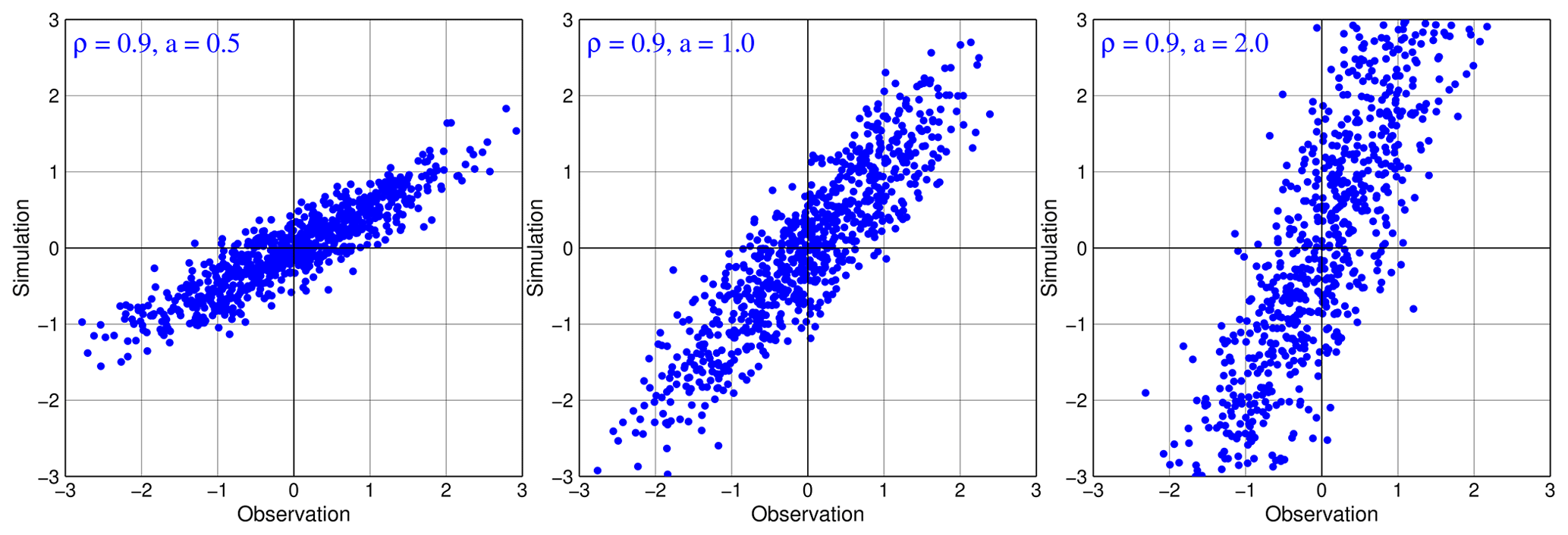
Figure 3 Joint probability distributions of simulations and observations with the same ρ=0.9 and different values of a in the mixed additive–multiplicative error model. Here, we assume b=0 and $o\sim \mathcal{N}(\mathrm{0},\mathrm{1})$; thus, the error model yields ${\mathit{\sigma }}_e=\sqrt{\mathrm{1}/{\mathit{\rho }}^{\mathrm{2}}-\mathrm{1}}a{\mathit{\sigma }}_o$. The noise levels, as measured by the generalized NSE, indicate the same noisiness for all forecasts, even though the noisiness seemingly increases with increasing a.

A further simple argument will show why the noise levels are the same in Fig. 3. Let us consider a simulation $s=o+\mathit{\epsilon }$. In this case, the simplest way to reduce the magnitude of the random error ε is to multiply s by a very small multiplicative factor a. By doing this, we have a new simulation $\stackrel{\mathrm{̃}}{s}=as$ with a new random error $\stackrel{\mathrm{̃}}{\mathit{\epsilon }}=a\mathit{\epsilon }$. Does this mean that $\stackrel{\mathrm{̃}}{s}$ is less noisy than s? Of course, this is not true at all, as the noisiness is measured by the relative magnitude between the power of noise and the power of the variation in observations but not by the absolute magnitude of noise. When we multiply s by a, we concurrently multiply o by a; as a result, the relative magnitude is unaltered. This further emphasizes that noisiness of all simulations $s=ao+a\mathit{\epsilon }$ for any value of a should be considered to be equivalent. The generalized NSE (Eq. 45) just reflects this fact.

As the upper bound of the generalized NSE is invariant when we introduce multiplicative biases into the additive error model (Eq. 7), all conclusions in Sect. 2.3 still hold. Thus, it is legitimate to use the upper bounds of the NDE and KGE, as expressed by Eqs. (23) and (26), respectively, in the general cases. This implies that the values NDE=0.5 and KGE≈0.5 remain to indicate the thresholds below which all simulations are considered to be poor. The generalized NDE and KGE can be derived using the same procedure to obtain Eqs. (29) and (30) with the generalized ${\text{NSR}}_{\mathrm{u}}=(b^{\mathrm{2}}+{\mathit{\sigma }}_e^{\mathrm{2}})/a^{\mathrm{2}}{\mathit{\sigma }}_o^{\mathrm{2}}$ in place of the traditional ${\text{NSR}}_{\mathrm{u}}=(b^{\mathrm{2}}+{\mathit{\sigma }}_e^{\mathrm{2}})/{\mathit{\sigma }}_o^{\mathrm{2}}$. We derive the generalized NDE for illustration:

$$\begin{array}{}\text{(47)}& \text{NDE}={\displaystyle \frac{\mathrm{1}}{\mathrm{1}+{\text{NSR}}_{\mathrm{u}}}}={\displaystyle \frac{a^{\mathrm{2}}{\mathit{\sigma }}_o^{\mathrm{2}}}{a^{\mathrm{2}}{\mathit{\sigma }}_o^{\mathrm{2}}+b^{\mathrm{2}}+{\mathit{\sigma }}_e^{\mathrm{2}}}}.\end{array}$$

It is worth noting that, when rewritten using the error model shown in Eq. (33), the variance term $({\mathit{\sigma }}_s/{\mathit{\sigma }}_o-\mathrm{1}{)}^{\mathrm{2}}$ will be replaced by $({\mathit{\sigma }}_s/a{\mathit{\sigma }}_o-\mathrm{1}{)}^{\mathrm{2}}$ in the form (Eq. 26) of the KGE_u:

$$\begin{array}{}\text{(48)}& \begin{array}{rl}{\text{KGE}}_{\mathrm{u}}& =\mathrm{1}-\sqrt{(\mathit{\rho }-\mathrm{1}{)}^{\mathrm{2}}+{\left({\displaystyle \frac{\mathrm{1}}{\mathit{\rho }}}-\mathrm{1}\right)}^{\mathrm{2}}}\\ & =\mathrm{1}-\sqrt{(\mathit{\rho }-\mathrm{1}{)}^{\mathrm{2}}+{\left({\displaystyle \frac{{\mathit{\sigma }}_s}{a{\mathit{\sigma }}_o}}-\mathrm{1}\right)}^{\mathrm{2}}}.\end{array}\end{array}$$

Combined with the generalized NSE_u (Eq. 46), we see that, in practice, if a is not taken into account (i.e., the traditional NSE and KGE are still used), we underestimate or overestimate the generalized NSE and KGE when a is smaller or greater than one, respectively.

In order to check the work of the generalized versions of the NSE, NDE, and KGE, we re-evaluate the performance of the two simulations in Eqs. (36) and (37). In the case of s₁, as the multiplicative bias a=1, the generalized efficiencies are identical to the traditional ones; therefore, we still have NSE₁=0, NDE₁=0.5, and KGE₁=0.5. As s₂ does not have any additive bias, its generalized NSE, NDE, and KGE are identical to its corresponding upper bounds:

$$\begin{array}{}\text{(49a)}& {\displaystyle }{\text{NSE}}_{\mathrm{2}}=\mathrm{1}-{\displaystyle \frac{{\mathit{\sigma }}_e^{\mathrm{2}}}{a^{\mathrm{2}}{\mathit{\sigma }}_o^{\mathrm{2}}}}=\mathrm{1}-{\displaystyle \frac{\stackrel{\mathrm{‾}}{(\mathrm{0.5}\mathit{\epsilon }{)}^{\mathrm{2}}}}{{\mathrm{0.5}}^{\mathrm{2}}{\mathit{\sigma }}_o^{\mathrm{2}}}}=\mathrm{1}-{\displaystyle \frac{{\mathrm{0.5}}^{\mathrm{2}}{\mathit{\sigma }}_o^{\mathrm{2}}}{{\mathrm{0.5}}^{\mathrm{2}}{\mathit{\sigma }}_o^{\mathrm{2}}}}=\mathrm{0},\text{(49b)}& {\displaystyle }\begin{array}{rl}{\text{NDE}}_{\mathrm{2}}& ={\displaystyle \frac{a^{\mathrm{2}}{\mathit{\sigma }}_o^{\mathrm{2}}}{a^{\mathrm{2}}{\mathit{\sigma }}_o^{\mathrm{2}}+{\mathit{\sigma }}_e^{\mathrm{2}}}}={\displaystyle \frac{{\mathrm{0.5}}^{\mathrm{2}}{\mathit{\sigma }}_o^{\mathrm{2}}}{{\mathrm{0.5}}^{\mathrm{2}}{\mathit{\sigma }}_o^{\mathrm{2}}+\stackrel{\mathrm{‾}}{(\mathrm{0.5}\mathit{\epsilon }{)}^{\mathrm{2}}}}}\\ & ={\displaystyle \frac{\mathrm{0.5}{\mathit{\sigma }}_o^{\mathrm{2}}}{\mathrm{0.5}{\mathit{\sigma }}_o^{\mathrm{2}}+\mathrm{0.5}{\mathit{\sigma }}_o^{\mathrm{2}}}}=\mathrm{0.5},\end{array}\text{(49c)}& {\displaystyle }\begin{array}{rl}{\text{KGE}}_{\mathrm{2}}& =\mathrm{1}-\sqrt{(\mathit{\rho }-\mathrm{1}{)}^{\mathrm{2}}+{\left({\displaystyle \frac{{\mathit{\sigma }}_{\mathrm{2}}}{a{\mathit{\sigma }}_o}}-\mathrm{1}\right)}^{\mathrm{2}}}\\ & =\mathrm{1}-\sqrt{{\left({\displaystyle \frac{\mathrm{0.5}{\mathit{\sigma }}_o}{\mathrm{0.5}\sqrt{\mathrm{2}}{\mathit{\sigma }}_o}}-\mathrm{1}\right)}^{\mathrm{2}}+{\left({\displaystyle \frac{\mathrm{0.5}\sqrt{\mathrm{2}}{\mathit{\sigma }}_o}{\mathrm{0.5}{\mathit{\sigma }}_o}}-\mathrm{1}\right)}^{\mathrm{2}}}\\ & \approx \mathrm{0.5}.\end{array}\end{array}$$

Thus, we obtain the same results as s₁, showing consistency between the two simulations, as expected.

With the generalized NSE, it is now possible to deal with the benchmark model s=μ_o. We exclude the trivial case $o=s={\mathit{\mu }}_o$ and always assume σ_o≠0. This special simulation is equivalent to the following model error:

$$\begin{array}{}\text{(50)}& s=\mathrm{0}\cdot o+{\mathit{\mu }}_o+\mathrm{0}.\end{array}$$

This implies a=0, b=μ_o, and σ_e=0 in Eq. (33). This specific error model highlights a problem that we have omitted when defining the generalized NSE: RNSR_u (Eq. 41), and therefore the NSE (Eq. 45), can only be defined for the cases a≠0. When a=0, simulations and observations are two uncorrelated signals (ρ=0) and it makes no sense to state that the received signal (simulations) is the true signal (observations) contaminated by noise.

In order to assign an appropriate value of the NSE for the cases ρ=0, we rely on the continuity of the NSE_u with respect to ρ, as shown in Eq. (46). Let ρ approach zero in Eq. (46), and we get the limit ${\text{NSE}}_{\mathrm{u}}=-\mathrm{\infty }$. As the NSE_u is the upper bound of the NSE, this entails $\text{NSE}=-\mathrm{\infty }$. The same argument yields NDE=0 and $\text{KGE}=-\mathrm{\infty }$ under the limit ρ→0. In other words, all simulations uncorrelated with observations (which include the observed mean) should be classified as the worst simulations with $\text{NSE}=-\mathrm{\infty }$. This can be justified by noting that information on the variation in observations is totally unknown if only an uncorrelated simulation is available. Therefore, the generalized NSE provides a new interpretation of the benchmark simulation s=μ_o. Rather than a benchmark marking the boundary between good and bad simulations, the observed mean is indeed the worst simulation, which can be beat by any simulations correlated with observations.

In order to clarify the aforementioned sophisticated problem, we summarize our arguments as follows:

• In the perspective of signal processing, the additive error model cannot deal with the benchmark model s=μ_o.

• In the additive error model, NSE=0 means that noise dominates informative signals, which is unrelated to the observed mean.

• The mixed additive–multiplicative model enables us to interpret the case of the observed mean when the multiplicative bias a=0.

• However, the traditional NSE is not robust to multiplicative biases. When we design a new score robust to multiplicative biases, the observed mean should be interpreted as the worst simulation which gives us no information on observation variability.

• Although the observed mean can be easily obtained in hydrological model calibration and seems to be reasonable as a benchmark, it makes no sense to choose the observed mean as a benchmark simulation from the signal-processing viewpoint of the NSE.

4 Conclusion

The Nash–Sutcliffe efficiency (NSE) is a widely used score in hydrology, but it is not common in the other environmental sciences. One of the reasons for its unpopularity is that its scientific meaning is somehow unclear in the literature. Many attempts to establish a solid foundation for the NSE from several viewpoints, such as linear regression, skill scores, and multiple-criteria scores, exist This study contributes to these previous works by approaching the NSE from the viewpoint of signal progressing. Thus, a simulation is viewed as a received signal containing a wanted signal (observations) contaminated by an unwanted signal (noise). This view underlines the important role of the error model between simulations and observations, which is usually implicit in our assumption. Thus, our approach follows Bayesian inference, in which an error model is formally defined and a goodness-of-fit measure is then derived (Mantovan and Todini, 2006; Vrugt et al., 2008). The rational is to avoid the use of the NSE as a predefined measure without an explicit error model, like in generalized likelihood uncertainty estimation (Beven and Binley, 1992), which has caused a long debate in the hydrology community (Mantovan and Todini, 2006; Stedinger et al., 2008).

By assuming an additive error model, it is easy to point out that the NSE is equivalent to an important quantity in signal processing: the signal-to-noise ratio. More precisely, the NSE measures the relative magnitude of the power of noise to the power of the variation in observations. Therefore, the NSE is a universal metric that should be applicable in any scientific field. However, due to its dependence on the power of the variation in observations, the NSE should not be used as a performance measure to compare different signals. Its scientific meaning suggests a natural way to choose NSE=0 as the threshold to distinguish between good and bad simulations in practice. This is because the power of noise starts dominating the power of the variation in observations when the NSE goes below zero, meaning that noise distorts the desired signal and makes it difficult to extract the useful information. This choice has no relation to the interpretation that NSE=0 corresponds to the benchmark simulation equal to the observed mean, and all good simulations need be better than this benchmark.

As the NSE can be easily increased simply by adding appropriate constants to simulations and observations, we seek its upper bound NSE_u using all such additions. The NSE_u is seen to correspond to the random component of the NSR and is a useful concept in analyzing the behavior of not only the NSE but also the NDE and KGE. It turns out that the NSE_u, NDE_u, and KGE_u are different measures of noisiness, which can be mapped one-to-one between any two scores. More surprisingly, it is found that these scores, in turn, can be expressed in terms of a more familiar quantity: the correlation coefficient. This implies that they do not introduce any new score and can equivalently be replaced by ρ. In this sense, any new score can be constructed from ρ with any monotonic function of ρ. This leads to an important finding: corresponding to NSE=0, we have NDE=0.5, KGE≈0.5 (not KGE=0), and ρ≈0.7, which mark the thresholds for good vs. bad model distinction. This has an important practical implication for the use of the KGE, as modelers usually identify KGE=0 for this threshold, similar to NSE=0. Thus, in practice, models with a KGE between 0 and 0.5 can be wrongly classified as showing good performance.

As the additive error model cannot describe the simulations that have variances smaller than the observation variances, we need to work with a more general error model to deal with such cases. By assuming a bivariate normal distribution between simulations and observations, the general error model is found to be the mixed additive–multiplicative error model. In the general cases, the traditional NSE is shown to be prone to contradictions: different evaluations of model performance can be drawn from a simulation by just scaling this simulation. Therefore, an extension of the NSE needs to be derived. By requiring that the generalized NSE is invariant in affine transformations of simulations and observations induced by the general error model, which helps to avoid any contradiction, the most appropriate form is found to be the traditional one adjusted by the multiplicative bias. Again, this has a practical implication on the use of the NSE and KGE: if the multiplicative factor is not taken into account and the traditional ones are used instead, both the scores are underestimated or overestimated when the multiplicative bias is greater than or smaller than one, respectively. The threshold values of NSE=0, NDE=0.5, KGE≈0.5, and ρ≈0.7 still hold with the generalized scores.

Finally, we summarize some profound explanations that the signal processing approach to the NSE proposes:

• Despite their different forms, the NSE, NDE, KGE, and the correlation coefficient are equivalent, at least when there are no biases, in the sense that they measure the noise-to-signal ratio between the power of noise and the power of the variation in observations.

• The threshold NSE=0 for good vs. bad model distinction follows naturally from the fact that the power of noise starts dominating the power of the variation in observations at this value. The choice of a benchmark model like the observed mean required in the interpretation of such a threshold in the traditional approach is no longer needed in the context of signal processing.

• Furthermore, the signal-processing-based approach seamlessly enables us to derive the corresponding thresholds for other scores (like the NDE and KGE) in the same manner, a problem which is not well defined if the benchmark approach is still followed. Corresponding to NSE=0, the thresholds of the KGE and the correlation coefficient are given by approximately 0.5 and 0.7, respectively.

• The traditional form of the NSE only reflects the noise-to-signal ratio in the additive error model. It no longer reflects this when multiplicative biases are introduced; as a result, it has an unintuitive form in the general cases.

• It is necessary to adjust the traditional NSE in the general cases to avoid potential contradictions in model evaluations. If the effect of multiplicative biases on the noise-to-signal ratio is not considered and the traditional NSE continues to be used, the NSE is underestimated or overestimated when the multiplicative bias is greater than or smaller than one, respectively.

• All simulations that are uncorrelated with observations are considered to be the worst simulations when measured by the NSE or KGE, as no information on the variation in observations can be retrieved in these cases. The constant simulation given by the observed mean s=μ_o belongs to this class of simulations. Therefore, in the view of signal processing, the observed mean should not be used as a benchmark model.