the Creative Commons Attribution 4.0 License.
the Creative Commons Attribution 4.0 License.
 | 09 May 2023
Benchmarking high-resolution hydrologic model performance of long-term retrospective streamflow simulations in the contiguous United States
Sydney S. Foks
Aubrey L. Dugger
Jesse E. Dickinson
Hedeff I. Essaid
David Gochis
Roland J. Viger
Yongxin Zhang
Because use of high-resolution hydrologic models is becoming more widespread and estimates are made over large domains, there is a pressing need for systematic evaluation of their performance. Most evaluation efforts to date have focused on smaller basins that have been relatively undisturbed by human activity, but there is also a need to benchmark model performance more comprehensively, including basins impacted by human activities. This study benchmarks the long-term performance of two process-oriented, high-resolution, continental-scale hydrologic models that have been developed to assess water availability and risks in the United States (US): the National Water Model v2.1 application of WRF-Hydro (NWMv2.1) and the National Hydrologic Model v1.0 application of the Precipitation–Runoff Modeling System (NHMv1.0). The evaluation is performed on 5390 streamflow gages from 1983 to 2016 (∼ 33 years) at a daily time step, including both natural and human-impacted catchments, representing one of the most comprehensive evaluations over the contiguous US. Using the Kling–Gupta efficiency as the main evaluation metric, the models are compared against a climatological benchmark that accounts for seasonality. Overall, the model applications show similar performance, with better performance in minimally disturbed basins than in those impacted by human activities. Relative regional differences are also similar: the best performance is found in the Northeast, followed by the Southeast, and generally worse performance is found in the Central and West areas. For both models, about 80 % of the sites exceed the seasonal climatological benchmark. Basins that do not exceed the climatological benchmark are further scrutinized to provide model diagnostics for each application. Using the underperforming subset, both models tend to overestimate streamflow volumes in the West, which could be attributed to not accounting for human activities, such as active management. Both models underestimate flow variability, especially the highest flows; this was more pronounced for NHMv1.0. Low flows tended to be overestimated by NWMv2.1, whereas there were both over and underestimations for NHMv1.0, but they were less severe. Although this study focused on model diagnostics for underperforming sites based on the seasonal climatological benchmark, metrics for all sites for both model applications are openly available online.
- Article
(10507 KB) - Full-text XML
-
Supplement
(6933 KB) - BibTeX
- EndNote


Across the hydrologic modeling community, there is a pressing need for more systematic documentation and evaluation of continental-scale land surface and streamflow model performance (Famiglietti et al., 2011). A challenge to hydrologic evaluation stems from the fact that the objectives of hydrologic modeling often vary. Archfield et al. (2015) reviewed how different communities have approached hydrologic modeling in the past, drawing a distinction between hydrologic catchment modelers, whose primary interest has been simulating streamflow at the local to regional scale, versus land surface modelers, who have historically focused on the water cycle as it relates to atmospheric and evaporative processes at the global scale. As modeling approaches have advanced toward coupled hydrologic and atmospheric systems, both perspectives have evolved and are converging towards the goal of improving hydrologic model performance through more intentional evaluation and benchmarking efforts.
Land surface modeling (LSM) has a rich history of community-developed benchmarking and intercomparison projects (van den Hurk et al., 2011; Best et al., 2015). In addition to comparative evaluations of process-based models, the LSM community has used statistical benchmarks, which in some cases have been shown to make better use of the forcing input data than state-of-the-art land surface models (Abramowitz et al., 2008; Nearing et al., 2018). The International Land Model Benchmarking (ILAMB) project is an international benchmarking framework developed by the LSM community (Luo et al., 2012) that has been applied to comprehensively evaluate Earth system models, including the categories of biogeochemistry, hydrology, radiation and energy, and climate forcing (Collier et al., 2018). Although hydrology is a component of ILAMB and other LSM benchmarking efforts, there is a need for closer collaboration with hydrologists to improve hydrologic process representation in these models (Clark et al., 2015).
Hydrologic catchment modeling has begun to move towards large-sample hydrology, an extension of comparative hydrology, where model performance is evaluated for a large sample of catchments, rather than focusing solely on individual watersheds. This is appealing because evaluating hydrologic models across a wide variety of hydrologic regimes facilitates more robust regional generalizations and comparisons (Gupta et al., 2014). As such, many hydrologic modeling evaluation efforts have begun to encompass larger spatial scales. Monthly water balance models have been used to relate model errors for the contiguous United States (CONUS) to hydroclimatic variables (Martinez and Gupta, 2010) as well as for parameter regionalization (Bock et al., 2016). As part of Phase 2 of the North American Land Data Assimilation System project, Xia et al. (2012) evaluated the simulated streamflow for four land surface models, focusing mostly on 961 small basins and 8 major river basins in the CONUS, finding that the ensemble mean performs better than the individual models. Further, several large-sample datasets have been developed for community use. The Model Parameter Estimation Experiment (MOPEX) includes hydrometeorological time series and land surface attributes for hydrological basins in the US and globally that have minimal human impacts (Duan et al., 2006). The more recent Catchment Attributes and Meteorology for Large-sample Studies (CAMELS) dataset includes hydrometeorological data and catchment attributes for more than 600 small- to medium-sized basins in the CONUS (Addor et al., 2017). By using CAMELS basins that are minimally disturbed by human activities, Newman et al. (2015, 2017) and Addor et al. (2018) were able to attribute regional variations in model performance to continental-scale factors. Knoben et al. (2020) also used CAMELS with 36 lumped conceptual models, finding that model performance is more strongly linked to streamflow signatures than to climate or catchment characteristics.
While these efforts are useful towards evaluating smaller, minimally impacted basins, there is also a need to benchmark model performance for larger basins, including those impacted by human activities. On the global scale, catchment techniques have been applied to global hydrologic modeling, and they have been shown to outperform traditional gridded global models of river flow (Arheimer et al., 2020). On the regional scale, Lane et al. (2019) benchmarked the predictive capability of river flow for over 1000 catchments in Great Britain by using four lumped hydrological models; they included both natural and human-impacted catchments, finding poor performance when the water budget was not closed, such as due to non-modeled human impacts. Mai et al. (2022b) conducted a systematic intercomparison study over the Great Lakes region, finding that regionally calibrated models suffer from poor performance in urban, managed, and agricultural areas. Tijerina et al. (2021) compared the performance of two high-resolution models that incorporate lateral subsurface flow at 2200 streamflow gages; they found poor performance in the central US, potentially due to non-modeled groundwater abstraction and irrigation, during a 1-year study period. As hydrologic model development moves to include human systems, these studies provide important baselines.
This study builds on previous large-sample studies by benchmarking long-term retrospective streamflow simulations over the CONUS. Specifically, two high-resolution, process-oriented models are evaluated that have been developed to address water issues nationally: the National Water Model v2.1 application of WRF-Hydro (NWMv2.1; Gochis et al., 2020a) and the National Hydrologic Model v1.0 application of the Precipitation–Runoff Modeling System (NHMv1.0; Regan et al., 2018). The evaluation is performed on daily streamflow for 5390 streamflow gages from 1983 to 2016 (∼ 33 years), including both natural and human-impacted catchments, representing one of the most comprehensive evaluations over the CONUS to date. The model performance is compared against a climatological benchmark that accounts for seasonality, and results are examined in terms of spatial patterns and human influences. The climatological seasonal benchmark is used as a threshold to screen the sites for each model application, offering a way to target the results for model diagnostics and development.
2.1 The National Water Model v2.1 application of WRF-Hydro (NWMv2.1)
The National Center for Atmospheric Research (NCAR) has developed an open-source, spatially distributed, physics-based community hydrologic model, WRF-Hydro (Gochis et al., 2020a, b), which is the current basis for the National Oceanic and Atmospheric Administration's National Water Model (NWM). The NWM is an operational hydrologic modeling system simulating and forecasting major water components (e.g., evapotranspiration, snow, soil moisture, groundwater, surface inundation, reservoirs, and streamflow) in real time across the CONUS, Hawaii, Puerto Rico, and the US Virgin Islands. NWM streamflow simulations from the version 2.1 CONUS long-term retrospective analysis (NWMv2.1) are used. The retrospective data are available from public cloud data outlets (e.g., compressed netCDF files can be found at https://noaa-nwm-retrospective-2-1-pds.s3.amazonaws.com/index.html). More information on these data is available from the Office of Water Prediction (OWP) National Water Model (OWP, 2022) and release notes (Farrar, 2021).
NWMv2.1 is forced by 1 km atmospheric states and fluxes from NOAA's Analysis of Record for Calibration (AORC; National Weather Service, 2021). For the land surface model, NWMv2.1 uses the Noah-MP (Noah-multiparameterization; Niu et al., 2011), which calculates energy and water states and vertical fluxes on a 1 km grid. WRF-Hydro physics-based hydrologic routing schemes transport surface water and shallow saturated soil water laterally across a 250 m resolution terrain grid and into channels. NWMv2.1 also leverages WRF-Hydro's conceptual baseflow parameterization, which approximates deeper groundwater storage and release through a simple exponential decay model. The three-parameter Muskingum–Cunge river routing scheme is used to route streamflow on an adapted National Hydrography Dataset Plus (NHDPlus) version-2 (McKay et al., 2012) river network representation (Gochis et al., 2020a). A level-pool scheme is activated on 5783 lakes and reservoirs across CONUS representing passive storage and releases from waterbodies; however, no active reservoir management is currently included in the NWM. While the operational NWM does include data assimilation, there is no data assimilation applied in the retrospective simulations used here. Using the AORC meteorological forcings, NWMv2.1 calibrates a subset of 14 soil, vegetation, and baseflow parameters to streamflow in 1378 gaged, predominantly natural flow basins. The calibration procedure uses the Dynamically Dimensioned Search algorithm (Tolson and Shoemaker, 2007) to optimize parameters to a weighted Nash–Sutcliffe efficiency (NSE; Nash and Sutcliffe, 1970) of hourly streamflow (mean of the standard NSE and log-transformed NSE). Calibration runs separately for each calibration basin, and a hydrologic similarity strategy is then used to regionalize parameters to the remaining basins within the model domain. The calibration period was from water years 2008 to 2013, and the water years from 2014 to 2016 were used for validation. For the retrospective analysis, NWMv2.1 produces the channel network output (streamflow and velocity), reservoir output (inflow, level, and outflow) and groundwater output (inflow, level, and outflow) every hour and every 3 h for land model output (e.g., snow, evapotranspiration, and soil moisture) and high-resolution terrain output (shallow water table depth, and ponded water depth). For this analysis, hourly streamflow is aggregated to daily averages.
2.2 The National Hydrologic Model v1.0 application of the Precipitation–Runoff Modeling System (NHMv1.0)
The U.S. Geological Survey (USGS) has developed the National Hydrologic Model (NHM, version 1.0) application of the Precipitation–Runoff Modeling System (PRMS) (Regan et al., 2018). PRMS uses a deterministic, physical-process representation of water flow and storage between the atmosphere and land surface, including snowpack, canopy, soil, surface depression, groundwater storage, and stream networks. Used here are the NHM daily discharge simulations from version v1.0 (NHMv1.0) and, more specifically, results from the calibration workflow “by headwater calibration using observed streamflow” with the Muskingum–Mann streamflow routing option (“byHRU_musk_obs”; Hay and LaFontaine, 2020).
Climate inputs to the NHMv1.0 are 1 km resolution daily precipitation and daily maximum and minimum temperature from Daymet (version 3; Thornton et al., 2016). The geospatial structure, which defines the default parameters, spatial hydrologic response units (HRUs), and the stream network, is defined by the geospatial fabric version 1.0 (Viger and Bock, 2014). The NHM is calibrated using a multiple-objective, stepwise approach to identify an optimal parameter set that balances water budgets and streamflow. The first step calibrates for the water balance of each spatial HRU to “baseline” observations of runoff, actual evapotranspiration, soil moisture, recharge, and snow-covered area derived from multiple datasets (Hay and LaFontaine, 2020). The second step considers timing of streamflow by calibration to statistically generated streamflow in 7265 headwater watersheds with a drainage area of less than 3000 km2. The final step calibrates to observed gaged streamflow at 1417 stream gage locations; details of the calibration can be seen in Appendix 1 of LaFontaine et al. (2019). The calibration period included the odd water years from 1981 to 2010, and the even water years from 1982 to 2010 were used for validation. The NHM does not simulate reservoir operations, surface or groundwater withdrawals, or stream releases. The NHM outputs daily streamflow, which is used in the analysis here.

Figure 1Site locations used in evaluation (n = 5390), including regions and classification. Regions were further combinations of the aggregated ecoregions defined by Falcone (2011): Central (n = 1450) includes the Central Plains, Western Plains, and Mixed Wood Shield; Northeast (n = 1218) includes the Northeast and Eastern Highlands; Southeast (n = 1212) includes the South East Plains and South East Coastal Plains; and West (n = 1510) includes the Western Mountains and West Xeric. Classifications are from Falcone (2011): reference (Ref, n = 1115) and non-reference (Non-ref, n = 4274); one gage was not designated (NA, n = 1). The map was sourced from Grannemann (2010), Natural Earth Data (2009), and Esri (2022a, b).
3.1 Data
This study evaluates daily simulations from 1 October 1983 to 31 December 2016, or just over 33 years (∼ 12 100 d). Model simulations are compared to observations at 5390 USGS stations (Foks et al., 2022); stations were included that had a minimum data length of at least 8 years or 2920 daily observations (i.e., ∼ 25 % complete data), although the observations did not need to be continuous (this allows for missing data, including intermittent and/or seasonally operated gages). A subset of these gages (n = 5389) also occurs in the Geospatial Attributes of Gages for Evaluating Streamflow, version II dataset (GAGES-II; Falcone, 2011); therefore, attributes from GAGES-II are used to examine select results. Figure 1 shows the spatial distribution of the gages as well as their designated region; regions are further aggregations of Level-II ecoregions as defined by GAGES-II (see Fig. 1 caption). Figure 1 shows the uneven distribution of gages: the eastern US has a dense network of gages, followed by decreasing coverage moving west around the 100th meridian (i.e., 100∘ W longitude). There is a modest increase in gage density across the intermountain west, and higher coverage along the west coast. Figure 1 also shows the classification – that is, if the site has been characterized as a reference or non-reference site. Reference gages indicate less-disturbed watersheds, and observations associated with non-reference gages have some level of anthropogenic influence (Falcone, 2011). Although the non-reference gages outnumber the reference gages by about 4 : 1, reference gages are relatively well-distributed through the regions.
Table 1Evaluation metrics calculated on the daily streamflows. The abbreviations used in the table are as follows: KGE – Kling–Gupta efficiency, rSD – ratio of standard deviations between simulations and observations, PBIAS – percent bias, HF – high flows, LF – low flows, Inf – infinity, USGS – United States Geological Survey, and m3 s−1 – cubic meters per second.
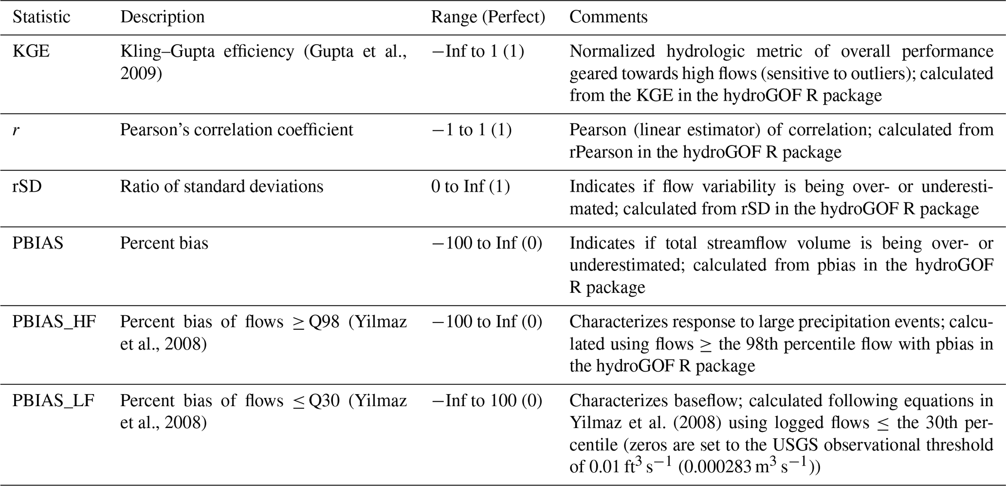
3.2 Metrics
Table 1 shows the metrics used in the evaluation as well as their descriptions. Metrics were calculated in the statistical software R (R Core Team, 2021), including using the hydroGOF (hydrological goodness-of-fit) package (Zambrano-Bigiarini, 2020).
The Kling–Gupta efficiency (KGE) is used as the overall performance metric, which is defined as follows (Gupta et al., 2009):
where r is the linear (Pearson) correlation coefficient between the observations (obs) and simulations (sim), σ is the standard deviation of the flows, and μ is the mean. The KGE components of r and the ratio of standard deviations between the simulations and observations (rSD) are also examined. Correlation quantifies the relationship between modeled and observed streamflow and is often used to assess flow timing. The rSD shows the relative variability (Gupta et al., 2009; Newman et al., 2017), indicating if the model is over- or underestimating the variability in the simulated state (in this case, daily streamflow), relative to observations. In this evaluation, instead of using the ratio of means component, the related percent bias (PBIAS) is calculated as follows (Zambrano-Bigiarini 2020):
where observed flow is O, simulated flow is S, and t = is the time series flow index. Percent bias (PBIAS) provides information on if the model is over- or underestimating the total streamflow volume (based on the entire simulation period).
To provide context for the interpretation of the KGE scores, a lower benchmark must be specified (Pappenberger et al., 2015; Schaefli and Gupta, 2007; Seibert, 2001; Seibert et al., 2018). The KGE does not include a built-in lower benchmark in its formulation, but Knoben et al. (2019) showed that models with KGE scores higher than −0.41 contribute more information than the mean flow benchmark. Recently, Knoben et al. (2020) showed that it is more robust to define a lower benchmark that considers seasonality. Hence, a reference time series based on the average and median flows for each day of the year is used to calculate a lower KGE value which serves as a climatological (lower) benchmark.
Two additional hydrologic signatures are included which evaluate performance based on different parts of the flow duration curve (FDC) for high and low flows. The definitions of these hydrologic signatures are consistent with those from Yilmaz et al. (2008). The bias of high flows (the top 2 %) is computed to evaluate how well the model captures the watershed response to big precipitation or melt events (PBIAS_HF). For low flows, the bias of the bottom 30 % (PBIAS_LF) offers insight into baseflow performance. Equations for these two metrics can be found in the online Supplement.
Table 2Median Kling–Gupta efficiency (KGE) scores and the percentage of sites (p) less than or greater than given KGE scores for seasonal benchmarks based on the median day-of-year flows (MedDOY) and average day-of-year flows (AvgDOY) and based on the National Water Model v2.1 (NWMv2.1) and National Hydrologic Model v1.0 (NHMv1.0).
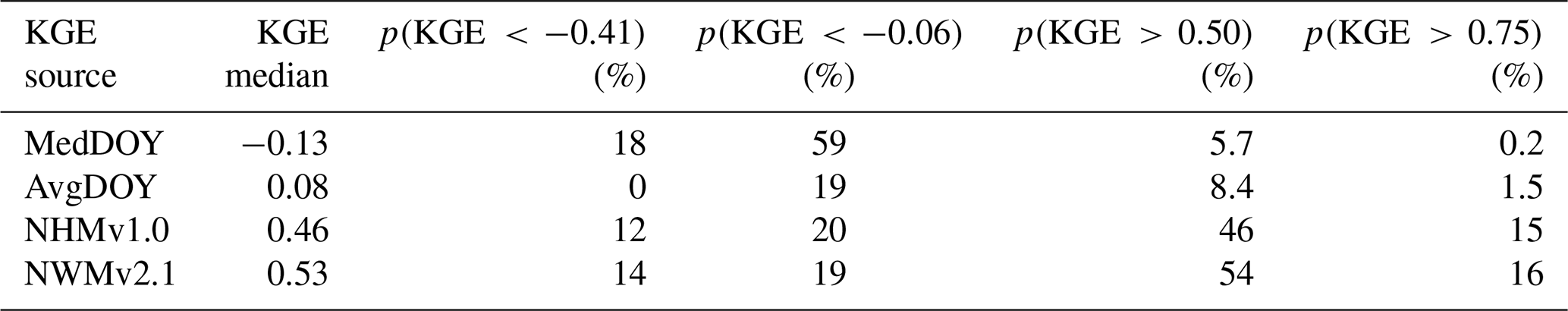

Figure 2Cumulative density functions (CDFs) for Kling–Gupta efficiency (KGE) scores based on daily streamflow at U.S. Geological Survey (USGS) gages for seasonal benchmarks based on the median day-of-year flows (MedDOY) and average day-of-year flows (AvgDOY) and based on the National Water Model v2.1 (NWMv2.1) and National Hydrologic Model v1.0 (NHMv1.0). The dotted vertical line is the KGE mean flow benchmark (−0.41). For sites (n = 1 for NWMv2.1 and n = 16 for NHMv1.0) for which a KGE could not be calculated (i.e., the modeled time series had all zero values for the entire time series), these are included as negative infinity in the CDFs.
Using daily observations and model simulations, the evaluation metrics from Table 1 are calculated for each of the gages for the NWMv2.1 (Towler et al., 2023a) and NHMv1.0 (Towler et al., 2023b) hydrologic modeling applications. As mentioned, to produce a seasonal climatological benchmark, KGE is also calculated using daily observations and day-of-year averages and medians for each site; these KGE scores are referred to as AvgDOY and MedDOY, respectively.
KGE scores for the benchmarks and models are presented as cumulative density functions (CDFs; Fig. 2), and Table 2 quantifies the percentage of sites less than or greater than select KGE scores. First, the seasonal benchmarks and model KGE scores can be compared to the mean flow benchmark (i.e., KGE < −0.41; Knoben et al., 2019): for the MedDOY, 18 % of sites have lower scores (Table 2). A total of 0 % of sites have lower scores than the KGE benchmark if the AvgDOY is used instead of the median flow (i.e., 0 % in Table 2). For the models, the NWMv2.1 simulations do not provide more skill than the mean flow benchmark at 14 % of the sites, similar to 12 % of sites using NHMv1.0. From Fig. 2, it can be seen that the CDFs for the models intersect with the AvgDOY curve at a KGE score of about −0.06; at this value, 19 %–20 % of the sites perform worse in terms of the KGE using the model simulation, whereas the model simulations perform better than the AvgDOY above this value. In terms of median values, the AvgDOY (MedDOY) has a median KGE of 0.08 (−0.1), while the NWMv2.1 has a median of 0.53 and the NHMv1.0 median is 0.46. Given the better performance of the AvgDOY compared with the MedDOY, only the AvgDOY is used as the lower benchmark in the forthcoming analyses.
KGE performance is also examined by whether the gage has been classified as reference or non-reference. Figure 3 shows KGE scores as CDFs for the models and the AvgDOY benchmark grouped by this classification. As expected, the AvgDOY curves are virtually identical regardless of classification. However, for both models, the reference gages outperform the non-reference gages. Table 3 shows the median values for the models: for the NHMv1.0, the KGE is 0.67 and 0.38 for the reference and non-reference, respectively; for the NWMv2.1, the KGE is 0.65 for the reference versus 0.49 for the non-reference. Looking at the components, the r values are the same for both model reference sites (0.78). For the PBIAS, the NHMv1.0 shows an underestimation for both reference and non-reference sites (−4.1 % and −5.7 %, respectively), but the NWMv2.1 underestimates (−4.0 %) at the reference sites and overestimates (5.3 %) at the non-reference sites.
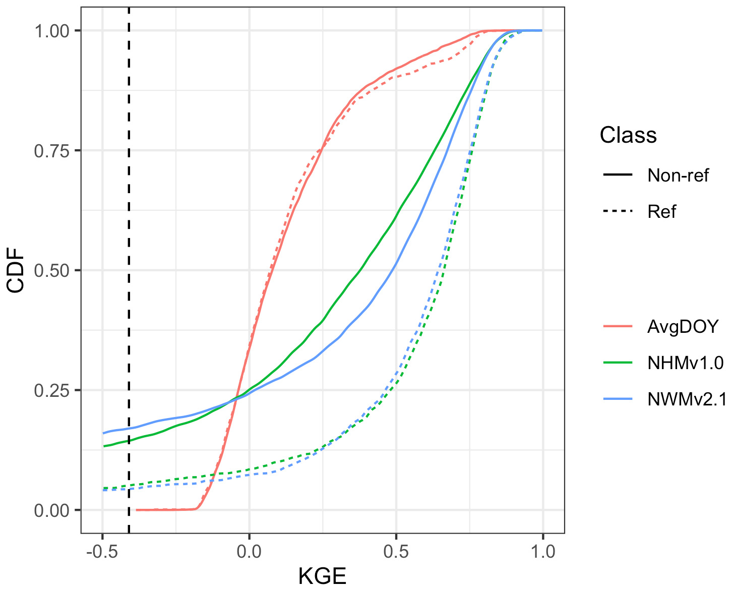
Figure 3Cumulative density functions (CDFs) for Kling–Gupta efficiency (KGE) scores based on daily streamflow at U.S. Geological Survey (USGS) gages for the seasonal benchmark based on average day-of-year flows (AvgDOY) and based on the National Water Model v2.1 (NWMv2.1) and National Hydrologic Model v1.0 (NHMv1.0). The dotted vertical line is the KGE mean flow benchmark (−0.41). Reference (Ref, n = 1115) and non-reference (Non-ref, n = 4274) classifications are from Falcone (2011).
Table 3Median values grouped by reference (Ref, n = 1115) and non-reference (Non-ref, n = 4274) gages (one gage was not designated as Ref or Non-ref and is, therefore, not included). The abbreviations used in the table are as follows: KGE – Kling–Gupta efficiency, r – Pearson's correlation coefficient, rSD – ratio of standard deviations between simulations and observations, PBIAS – percent bias, NHMv1.0 – National Hydrologic Model v1.0, and NWMv2.1 – National Water Model v2.1.

Figure 4 shows KGE scores as CDFs for the models grouped by region. The model applications are similar, but there are notable differences by region. In general, performance is best for the Northeast, followed by the Southeast. The Central and West areas perform the worst, although the West exhibits some high KGE values. Table 4 displays the median KGE, r, rSD, and PBIAS values grouped by region, showing the biggest differences in PBIAS among regions and between models. Regional variability can be further examined using the KGE maps for the models: in the West, more of the poorly performing sites are in the arid southwest and the lower-elevation basins in the intermountain west; better performance is seen at higher elevations in the intermountain west and along the west coast, including the Pacific Northwest (Fig. 5a for NWMv2.1 and Fig. 5b for NHMv1.0). Figure 5 shows that, for both models in the Central region, relatively poor performance is concentrated along the plains areas that span from the high plains (i.e., North Dakota) vertically down through the center of the CONUS (i.e., South Dakota, Nebraska, Kansas, and Texas). Performance is more mixed as one moves further east in the Central region (e.g., around the Great Lakes). Relatively good performance is seen in most of the Southeast, but performance tends to be poor or mixed in Florida. However, as previously mentioned, the model results need to be placed into context by comparing them to a climatological benchmark. Figure 6 shows the KGE map for the AvgDOY, which has relatively high KGE values mostly in parts of the western CONUS, where there are notable seasonal signatures (e.g., snowmelt runoff), and relatively low KGE values in most of the other regions. By taking the KGE differences by site, it is easier to examine where the model applications are relatively better or worse than the seasonal benchmark. Figure 7 shows the spatial distribution of the KGE differences, where the model with the maximum KGE value is used (i.e., maximum between the KGENWMv2.1 and KGENHMv1.0). Overall, the model applications tend to outperform the AvgDOY benchmark, except in the West and western Central regions. Figure S1 in the Supplement shows that if the AvgDOY benchmark is outperformed, it is usually by both models (at 63 % of sites); this is similar to the findings of Knoben et al. (2020). KGE difference maps for each individual model follow the same general spatial pattern (Figs. S2, S3).
Table 4Median values for each region. The abbreviations used in the table are as follows: KGE – Kling–Gupta efficiency, r – Pearson's correlation coefficient, rSD – ratio of standard deviations between simulations and observations, PBIAS – percent bias, NHMv1.0 – National Hydrologic Model v1.0, and NWMv2.1 – National Water Model v2.1.
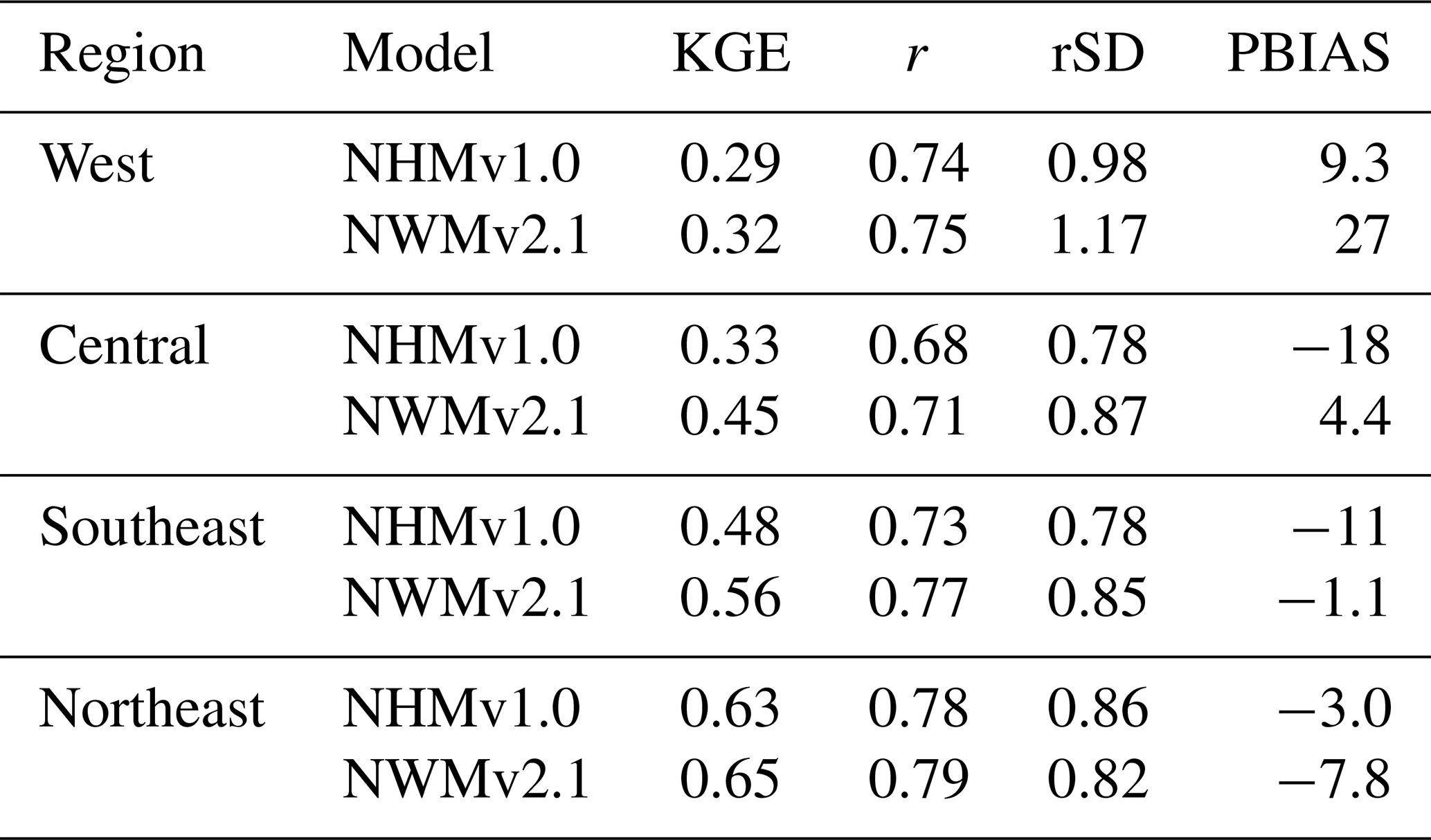
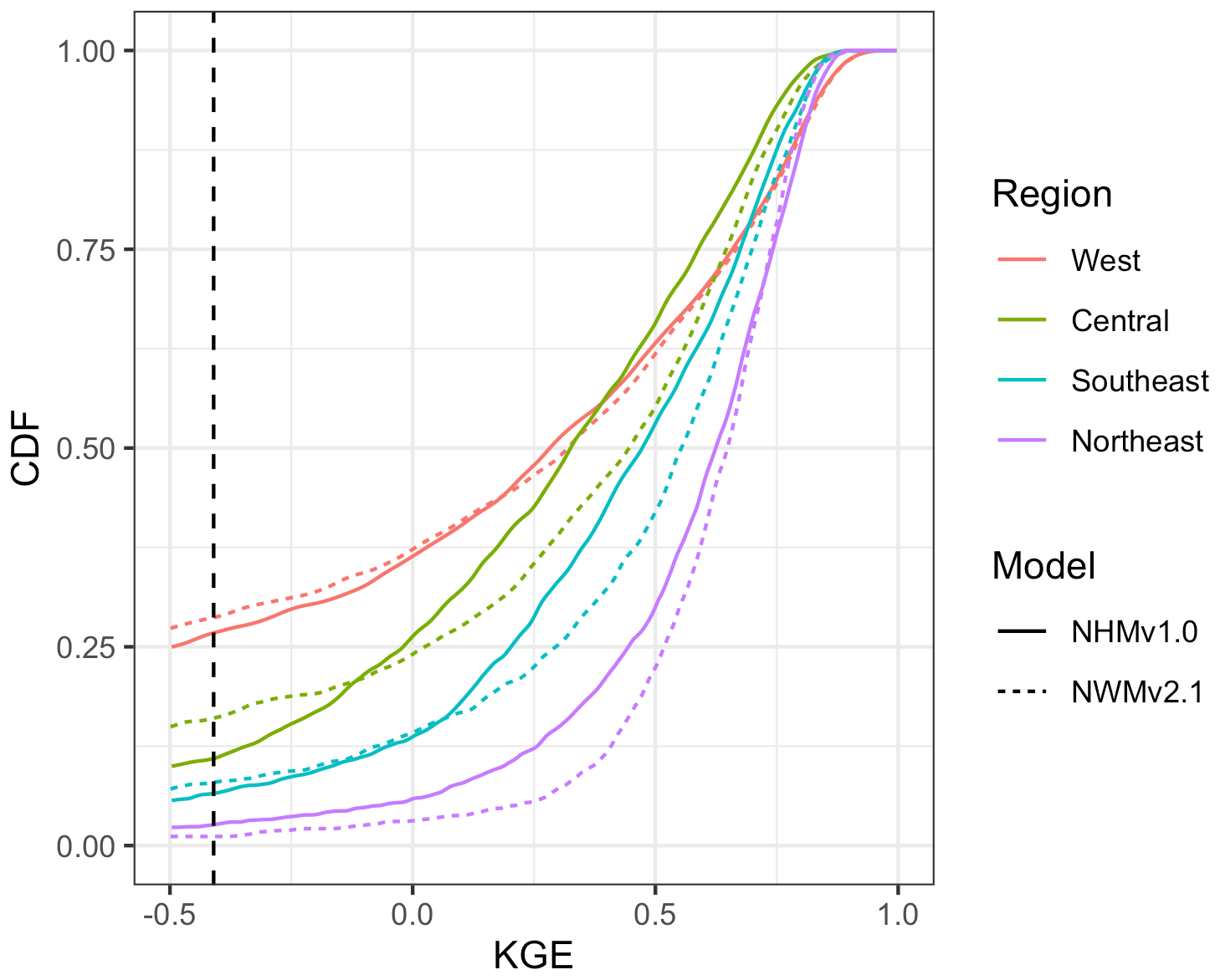
Figure 4Cumulative density functions (CDFs) for Kling–Gupta efficiency (KGE) scores based on the daily streamflow at U.S. Geological Survey (USGS) gages for the National Water Model v2.1 (NWMv2.1) and National Hydrologic Model v1.0 (NHMv1.0). The dotted vertical line is the KGE mean flow benchmark (−0.41). Regions are further combinations of the aggregated ecoregions defined by Falcone (2011): Central (n = 1450) includes the Central Plains, Western Plains, and Mixed Wood Shield; Northeast (n = 1218) includes the Northeast and Eastern Highlands; Southeast (n = 1212) includes the South East Plains and South East Coastal Plains; and West (n = 1510) includes the Western Mountains and West Xeric.
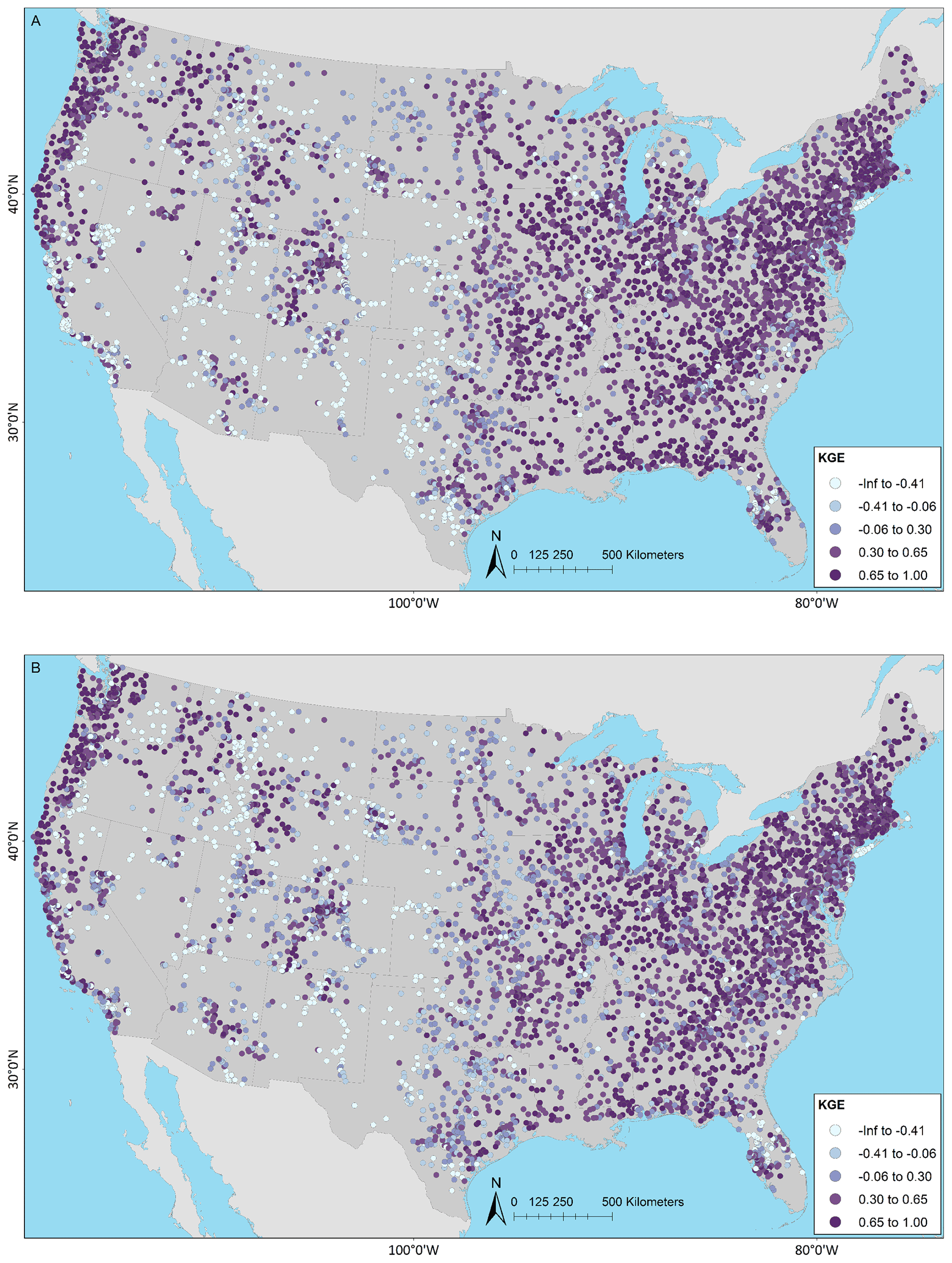
Figure 5Kling–Gupta efficiency (KGE) based on daily streamflow at U.S. Geological Survey (USGS) gages for the (a) National Water Model v2.1 (NWMv2.1) and (b) National Hydrologic Model v1.0 (NHMv1.0). The map was sourced from Grannemann (2010), Natural Earth Data (2009) and Esri (2022a, b).
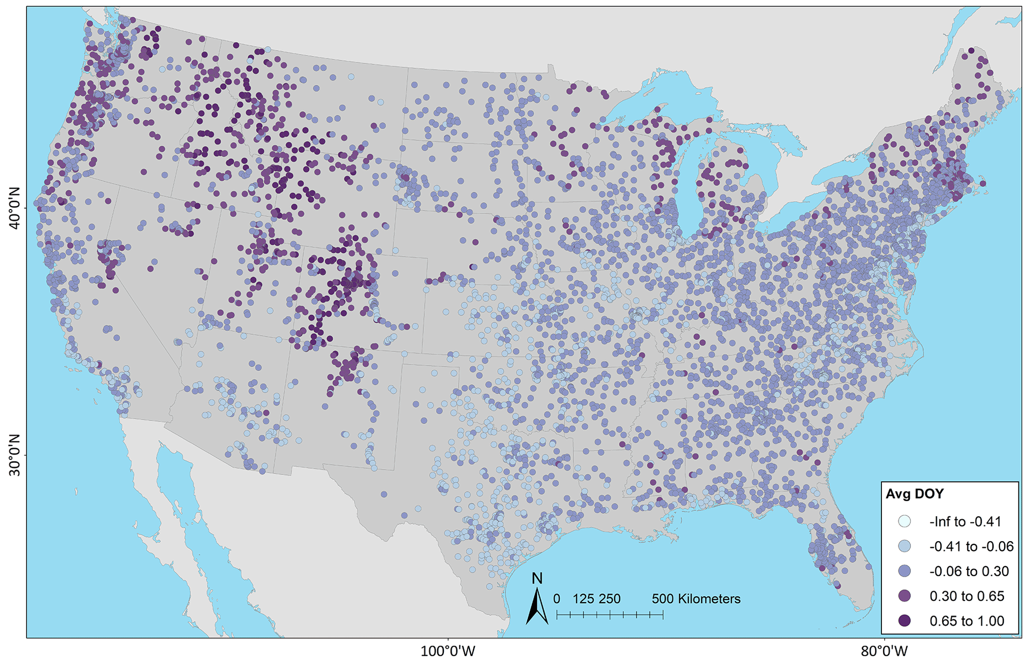
Figure 6Kling–Gupta efficiency (KGE) based on daily streamflow at U.S. Geological Survey (USGS) gages using the seasonal benchmark from average day-of-year flows (AvgDOY). The map was sourced from Grannemann (2010), Natural Earth Data (2009) and Esri (2022a, b).
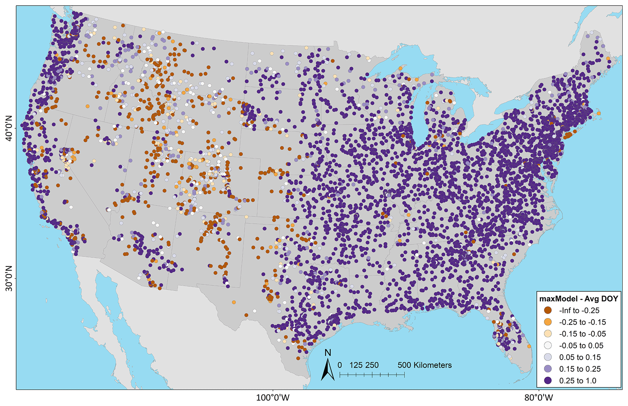
Figure 7Difference between the Kling–Gupta efficiency (KGE) from the maximum model (maxModel) (i.e., the maximum KGE value from the National Water Model v2.1, NWMv2.1, or the National Hydrologic Model v1.0, NHMv1.0) minus the seasonal benchmark based on the average day-of-year flows (AvgDOY); negative (orange) indicates where the AvgDOY has a higher (better) KGE, whereas positive (purple) indicates that at least one of the models has a higher (better) KGE. The map was sourced from Grannemann (2010), Natural Earth Data (2009) and Esri (2022a, b).
Basins that do not exceed the climatological benchmark are further scrutinized for each model application to offer insights for model diagnostics and development; that is, only sites that have KGE scores worse than the AvgDOY benchmark are examined hereafter. From here forward, these are called “underperforming sites”. By classification, most underperforming sites are human impacted (90 %–93 %; see Table 5). By region, most underperforming sites are in the West (55 %–67 %) or Central (23 %–28 %) regions (Table 6). Next, the bias metrics can be examined to try to determine why these sites are not able to beat the climatological benchmark. Spatial maps of PBIAS show that the NWMv2.1 (Fig. 8a) generally overestimates volume; NHMv1.0 (Fig. 8b) is more mixed with underestimation in the Central region. Both models overestimate water volumes in the West. This could be because neither model is capturing active reservoir operations or water extractions (e.g., for irrigation), which are important because water is heavily managed in the west. This is different from the overall distribution of PBIAS for the modeling applications, where, if one looks at all the gages (n = 5390), PBIAS for both models is centered around zero (Fig. S4). The underestimation in the Central region for the NHMv1.0, which is absent in NWMv2.1, could be due to the different time steps of the models – NWMv2.1 is run hourly and NHMv1.0 is run daily; this hypothesis is expanded upon in Sect. 5. Maps for PBIAS_HF can be seen in Fig. S5; for PBIAS_HF, the overall distribution of PBIAS_HF is centered below zero, indicating that the models tend to underestimate high flows, but this is more pronounced for the underperforming gages in the NHMv1.0 than in the NWMv2.1 (Fig. S6). Results for rSD paint a similar picture: both models tend to underestimate variability, but the underestimation is more pronounced in NHMv1.0 (Figs. S7, S8). Figure 9 shows PBIAS_LF for both model applications: the NWMv2.1 tends to overestimate the low flows, whereas the NHMv1.0 is more mixed and the over- or underestimation is less severe. This can also be seen in the histograms for PBIAS_LF (Fig. S9).
Table 5The number (percentage) of sites in each classification for each hydrologic model application where the KGE score is less than the average day-of-year flow (AvgDOY) benchmark (underperforming sites). The abbreviations used in the table are as follows: NHMv1.0 – National Hydrologic Model v1.0, NWMv2.1 – National Water Model v2.1, max(Model) – model with maximum KGE value from NHMv1.0 or NWMv2.1, Ref – reference (minimal human impacts), and Non-ref – non-reference (influenced by human activities).
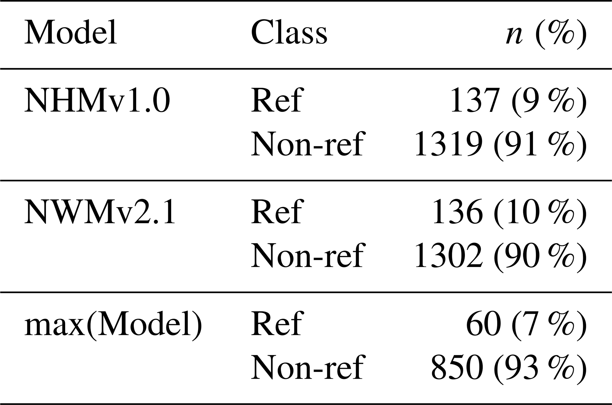
Table 6The number (percentage) of sites in each region for each hydrologic model application where the KGE score is less than the average day-of-year flow (AvgDOY) benchmark (underperforming sites). The abbreviations used in the table are as follows: NHMv1.0 – National Hydrologic Model v1.0, NWMv2.1 – National Water Model v2.1, and max(Model) – model with maximum KGE value from NHMv1.0 or NWMv2.1.
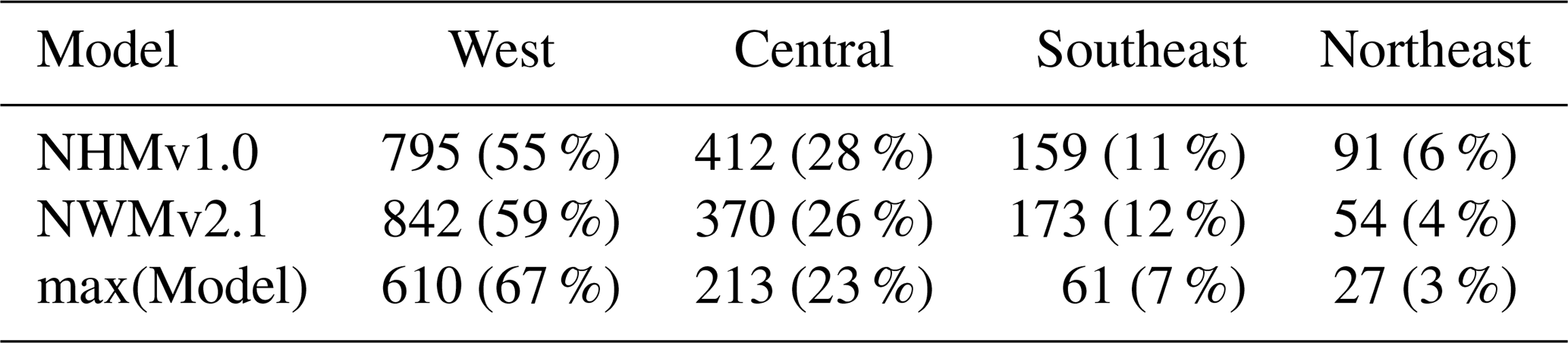
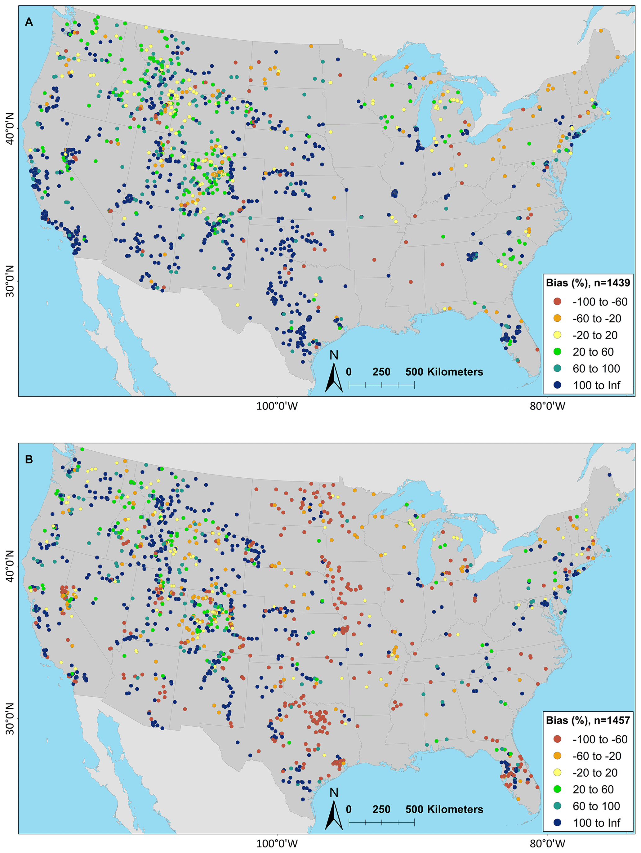
Figure 8Percent bias (PBIAS) maps for the (a) National Water Model v2.1 (NWMv2.1) and (b) National Hydrologic Model v1.0 (NHMv1.0) for sites where the KGE score is less than the average day-of-year flow (AvgDOY) benchmark. Cooler colors are where the model application is overestimating volume, whereas warmer colors are where the model is underestimating volume. The map was sourced from Grannemann (2010), Natural Earth Data (2009) and Esri (2022a, b).
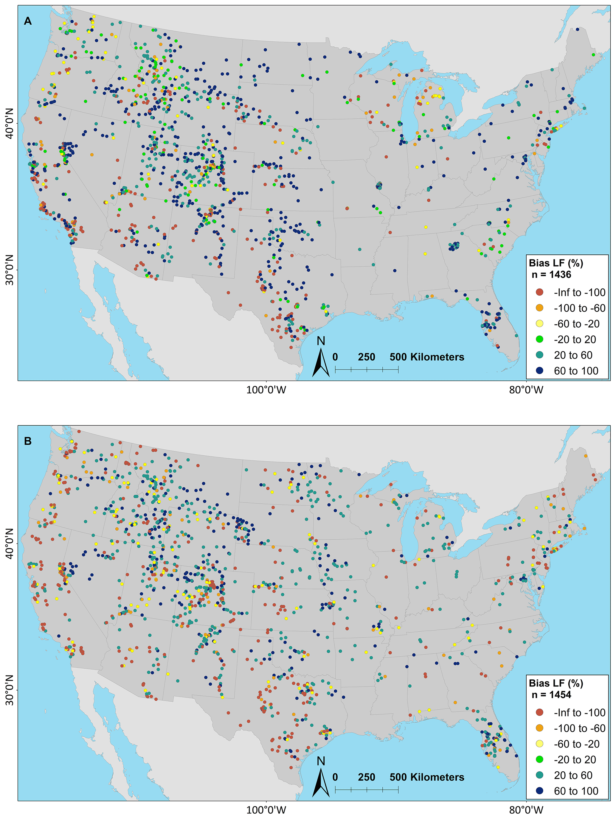
Figure 9Percent bias low flow (PBIAS_LF, flows below the 30 % percentile) maps for the (a) National Water Model v2.1 (NWMv2.1) and (b) National Hydrologic Model v1.0 (NHMv1.0) for sites where the KGE score is less than the average day-of-year flow (AvgDOY) benchmark. Cooler colors are where the model application is overestimating low flows, whereas warmer colors are where the model is underestimating low flows. The map was sourced from Grannemann (2010), Natural Earth Data (2009) and Esri (2022a, b).
Water availability is a critical concern worldwide; its assessment extends beyond the individual catchment scale and needs to include both large and small basins as well as anthropogenically influenced basins and those devoid of human influence. As such, large-sample hydrologic modeling and evaluation has taken on a new urgency, especially as these models are used to assess water availability and risks. In the US, the high-resolution model applications benchmarked here are two widely used federal hydrologic models, providing information at spatial and temporal scales that are vital to realizing water security. To our knowledge, this is the first time that these models have been evaluated so comprehensively, as this analysis included daily simulations at 5390 gages, over a 33-year period, and basins both impacted and not impacted by human activities. Further, a climatological seasonal benchmark is used to provide an a priori expectation of what constitutes as a “good” model. This analysis is aligned with the recent aims of the hydrologic benchmarking community to put performance metrics in context (Clark et al., 2021; Knoben et al., 2020). This paper extends this approach by demonstrating how the climatological benchmark can be used as a threshold to further scrutinize errors at underperforming sites. This is complementary to other model diagnostic and development work that aims to understand model sensitivity and why models improve/degrade with changes. Recent studies have applied sensitivity analyses that consider both parametric and structural uncertainties to identify the water cycle components that streamflow predictions are most sensitive to (Mai et al., 2022a). Information theory also provides tools that help identify model components contributing to errors (Frame et al., 2021). Further, simple statistical or conceptual models (e.g., Nearing et al., 2018; Newman et al., 2017) could also be used as a benchmark if applied to the same sites/catchments and time periods.
In terms of the KGE, the model applications showed similar performance, despite differences in process representations, parameter estimation strategies, meteorological forcings, and space/time discretizations. Reference gages performed better than the non-reference gages, and the best regional performance was seen in the Northeast, followed by the Southeast, with worse performance in the Central and West areas, although the West presented some high KGE scores. Further, for both models, most of the sites were able to beat the seasonal benchmark, and the majority of sites that did not were non-reference. Despite different forcings (NWMv2.1 is forced by AORC and NHMv1.0 is forced by Daymet version 3), the model applications had generally similar performance. Although outside the scope of this study, further exploration of streamflow biases due to forcing biases could offer insights into error sources. Moreover, the calibration periods of the models differed, and both overlapped with the evaluation period used in this study. While this overlap can introduce biases into the evaluation process, it allowed us to evaluate long-term performance for the same sites and time periods for both models. While this is not without precedent (e.g., Duan et al., 2006), recent studies are exploring best practices for calibration and validation to improve model robustness and generalizability (Shen et al., 2022).
PBIAS results showed that simulated streamflow volumes are overestimated in the West region for both models, particularly for the sites designated as non-reference. Lane et al. (2019) found that poor model performance occurs when the water budget is not closed, such as when human modifications or groundwater processes are not accounted for in the models. This is a likely explanation in our case as well, because water withdrawal for human use is endemic throughout the west and neither model has a thorough representation of these withdrawals. Furthermore, neither model possesses significant representations of lake and stream channel evaporation which, through the largely semiarid west, can constitute a significant amount of water “loss” to the hydrologic system (Friedrich et al., 2018). Lastly, nearly all western rivers are also subject to some form of impoundment. Even neglecting evaporative, seepage, and withdrawal losses from these waterbodies, the storage and timed releases of water from managed reservoirs can significantly alter flow regimes from daily to seasonal timescales, thereby degrading model performance statistics at gaged locations downstream of those reservoirs. As model development moves towards including human systems, the benchmark results provide a concrete goal regarding “how much” improvement could be necessary to achieve by a management module. This addition of management could support decision makers as they grapple with how to account for the anthropogenic influence on watersheds, especially as most studies to date focus on minimally disturbed sites.
Another interesting difference in PBIAS was seen in the Central US, where the NHMv1.0 underestimates volumes at underperforming sites. As detailed in the model descriptions, the model applications are run at different temporal scales: NHMv1.0 is run daily, whereas NWMv2.1 is run hourly and aggregated to daily. One hypothesis is that some precipitation events that are occurring on sub-daily scales, like convective storms and the associated runoff modes (Buchanan et al., 2018), may be missed. Similarly, while both models tend to underestimate high flows (PBIAS_HF) and variability (rSD), this is more pronounced for the NHMv1.0, which is in line with this hypothesis. The model applications showed differences in PBIAS_LF, with the NWMv2.1 overestimating low flows and the NHMv1.0 both over- and underestimated them, although the latter over- and underestimations were less severe. Both models used in the applications benchmarked here have only rudimentary representation of groundwater processes. Additional attributes (e.g., baseflow or aridity indices) could be strategically identified to further understand these model errors and differences. Model target applications, which drive model developer selections for process representation, space and time discretization, and calibration objectives, also have a notable imprint on the performance. The NWMv2.1, with a focus on flood prediction and fast (hourly) timescales, shows better performance for high-flow-focused metrics, whereas the NHMv1.0, designed for water availability assessment and slower (daily) timescales, shows more balanced and better performance for low-flow-focused metrics.
Identifying a suite of evaluation metrics has an element of subjectivity, but our aim was to focus on streamflow magnitude, as these model applications were developed to inform water availability assessments. However, magnitude is only one aspect of streamflow, and different metrics for other categories (e.g., frequency, duration, and rate of change) could be more appropriate for addressing specific scientific questions or modeling objectives. Recently, McMillan (2019) linked hydrologic signatures to specific processes using only streamflow and precipitation. The aforementioned publication did not find many signatures that relate to human alteration; however, in this paper, the streamflow bias metrics are found to be useful in this regard. Clark et al. (2021) pointed out that it is important to characterize the sensitivity of the KGE to sampling uncertainty, which can be large for heavy-tailed streamflow errors. Using bootstrap methods (Clark et al., 2021), uncertainty in the KGE estimates for this study were computed (Towler et al., 2023a, b) and are illustrated in Fig. S11. Alternative estimators of the KGE that are more appropriate for skewed streamflow data (e.g., see Lamontagne et al., 2020) could be added in the future, but they currently require the separate treatment of sites with zero streamflow, which was not feasible for this initial evaluation. Finally, some of the metrics in the benchmark suite include redundant error information; one approach to remedy this has been put forth by Hodson et al. (2021), where the mean log square error is decomposed to only include independent error components (see Hodson et al., 2021, for details). This could also be addressed using empirical orthogonal function (EOF) analysis, which has been done for climate model evaluation (Rupp et al., 2013).
In closing, this paper uses the climatological seasonal benchmark as a threshold to screen sites for each model application. While this fit with the purpose of this study, the metrics for NWMv2.1 (Towler et al., 2023a) and NHMv1.0 (Towler et al., 2023b) are available for all sites (Foks et al., 2022); these can be analyzed and/or screened as needed. In the future, it could also be useful to extend the analysis beyond streamflow to other water budget components to assess additional aspects of model performance.
NWMv2.1 model data can be accessed through an Amazon S3 bucket (https://registry.opendata.aws/nwm-archive/; NOAA, 2023), and NHMv1.0 model data are available as a USGS data release (https://doi.org/10.5066/P9PGZE0S; Hay and LaFontaine, 2020). Metrics discussed in this publication can be found at https://doi.org/10.5066/P9QT1KV7 (Towler et al., 2023a) and https://doi.org/10.5066/P9DKA9KQ (Towler et al., 2023b).
The supplement related to this article is available online at: https://doi.org/10.5194/hess-27-1809-2023-supplement.
ET and SSF collaborated to develop and demonstrate the evaluation and study design; ALD, JED, HIE, DG, and RJV contributed to discussions that shaped the ideas. ET led the analysis of results and prepared the original paper and revisions. All authors helped with the editing and revisions of the paper. YZ ran the NWM model and provided the data.
The contact author has declared that none of the authors has any competing interests.
Any use of trade, firm, or product names is for descriptive purposes only and does not imply endorsement by the US Government.
Publisher's note: Copernicus Publications remains neutral with regard to jurisdictional claims in published maps and institutional affiliations.
The authors are grateful to the USGS HyTEST evaluation team (Robert W. Dudley, Krista A. Dunne, Glenn A. Hodgkins, Timothy O. Hodson, Sara B. Levin, Thomas M. Over, Colin A. Penn, Amy M. Russell, Samuel W. Saxe, and Caelan E. Simeone), for feedback on the development of the evaluation and study design, and the WRF-Hydro group (in particular Ryan Cabell, Andy Gaydos, Alyssa McCluskey, Arezoo Rafieeinasab, Kevin Sampson, and Tim Schneider). We thank Stacey Archfield and Andrew Newman for comments on an earlier version of the paper.
This research was supported by the US Geological Survey (USGS) Water Mission Area's Integrated Water Prediction Program. The National Center for Atmospheric Research (NCAR) is a major facility sponsored by the National Science Foundation (NSF) under Cooperative Agreement 1852977.
This paper was edited by Christa Kelleher and reviewed by Robert Chlumsky and two anonymous referees.
Abramowitz, G., Leuning, R., Clark, M., and Pitman A. J.: Evaluating the performance of land surface models, J. Climate, 21, 5468–5481, 2008.
Addor, N., Newman, A. J., Mizukami, N., and Clark, M. P.: The CAMELS data set: catchment attributes and meteorology for large-sample studies, Hydrol. Earth Syst. Sci., 21, 5293–5313, https://doi.org/10.5194/hess-21-5293-2017, 2017.
Addor, N., Nearing, G., Prieto, C., Newman, A. J., Le Vine, N., and Clark, M. P.: A ranking of hydrological signatures based on their predictability in space, Water Resour. Res., 54, 8792–8812, https://doi.org/10.1029/2018WR022606, 2018.
Archfield, S. A., Clark, M., Arheimer, B., Hay, L. E., Mcmillan, H., Kiang, J. E., Seibert, J., Hakala, K., Bock, A., Wagener, T., Farmer, W.H., Andreassian, V., Attinger, S., Viglione, A., Knight, R., Markstrom, S., and Over, T.: Accelerating advances in continental domain hydrologic modeling, Water Resour. Res., 10078–10091, https://doi.org/10.1002/2015WR017498, 2015.
Arheimer, B., Pimentel, R., Isberg, K., Crochemore, L., Andersson, J. C. M., Hasan, A., and Pineda, L.: Global catchment modelling using World-Wide HYPE (WWH), open data, and stepwise parameter estimation, Hydrol. Earth Syst. Sci., 24, 535–559, https://doi.org/10.5194/hess-24-535-2020, 2020.
Best, M. J., Abramowitz, G., Johnson, H. R., Pitman, A. J., Balsamo, G., Boone, A., Cuntz, M., Decharme, B., Dirmeyer, P. A., Dong, J., Ek, M., Guo, Z., Haverd, V., van den Hurk, B. J. J., Nearing, G. S., Pak, B., Peters-Lidard, C., Santanello Jr., J. A., Stevens, L., and Vuichard, N.: The plumbing of land surface models: Benchmarking model performance, J. Hydrometeorol., 16, 1425–1442, https://doi.org/10.1175/JHM-D-14-0158.1, 2015.
Bock, A. R., Hay, L. E., McCabe, G. J., Markstrom, S. L., and Atkinson, R. D.: Parameter regionalization of a monthly water balance model for the conterminous United States, Hydrol. Earth Syst. Sci., 20, 2861–2876, https://doi.org/10.5194/hess-20-2861-2016, 2016.
Buchanan, B., Auerbach, D. A., Knighton, J., Evensen, D., Fuka, D. R., Easton, Z. Wieczorek, M., Archibald, J. A., McWilliams, B., and Walter, T.: Estimating dominant runoff modes across the conterminous United States, Hydrol. Process., 32, 3881–3890, https://doi.org/10.1002/hyp.13296, 2018.
Clark, M. P., Fan, Y., Lawrence, D. M., Adam, J. C., Bolster, D., Gochis D. J., Hooper, R. P., Kumar, M., Leung, L. R., Mackay, D. S., Maxwell, R. M., Shen, C., Swenson, S. C., and Zeng, X.: Improving the representation of hydrologic processes in Earth System Models, Water Resour. Res., 51, 5929–5956, https://doi.org/10.1002/2015WR017096, 2015.
Clark, M. P., Vogel, R. M., Lamontagne, J. R., Mizukami, N., Knoben, W. J. M., Tang, G., Gharari, S., Freer, J. E., Whitfield, P. H., Shook, K. R., and Papalexiou, S. M.: The abuse of popular performance metrics in hydrologic modeling, Water Resour. Res., 57, e2020WR029001, https://doi.org/10.1029/2020WR029001, 2021.
Collier, N., Hoffman, F. M., Lawrence, D. M., Keppel-Aleks, G., Koven, C. D., Riley, W. J., Mu, M., and Randerson, J. T.: The International Land Model Benchmarking (ILAMB) System: Design, Theory, and Implementation, J. Adv. Model. Earth Sy., 10, 2731–2754, https://doi.org/10.1029/2018MS001354, 2018.
Duan, Q., Schaake, J., Andréassian, V., Franks, S., Goteti, G., Gupta, H. V., Gusev, Y. M., Habets, F., Hall, A., Hay, L., Hogue, T., Huang, M., Leavesley, G., Liang, X., Nasonova, O. N., Noilhan, J., Oudin, L., Sorooshian, S., Wagener, T., and Wood, E. F.: Model parameter estimation experiment (MOPEX): An overview of science strategy and major results from the second and third workshops, J. Hydrol., 320, 3–17, https://doi.org/10.1016/j.jhydrol.2005.07.031, 2006.
Esri: USA States Generalized Boundaries, Esri [data set], https://esri.maps.arcgis.com/home/item.html?id=8c2d6d7df8fa4142b0a1211c8dd66903 (last access: 4 May 2023), 2022a.
Esri: World Countries (Generalized), Esri [data set], https://hub.arcgis.com/datasets/esri::world-countries-generalized/about (last access: 4 May 2023), 2022b.
Falcone, J. A.: GAGES-II: Geospatial attributes of gages for evaluating streamflow, US Geological Survey, https://doi.org/10.3133/70046617, 2011.
Famiglietti, J. S., Murdoch, L., Lakshmi, V., Arrigo, J., and Hooper, R.: Establishing a Framework for Community Modeling in Hydrologic Science, 3rd Workshop on Community Hydrologic Modeling Platform (CHyMP), 15–17 March 2011, University of California, Irvine, https://www.hydroshare.org/resource/2b8c9e2ecf014cf284278b1784b16570/data/contents/CUAHSI-TR10_-_Establishing_a_Framework_for_Community_Modeling_in_Hydrologic_Science_-_2011.pdf (last access: 4 May 2023), 2011.
Farrar, M.: Service Change Notice, https://www.weather.gov/media/notification/pdf2/scn20-119nwm_v2_1aad.pdf (last access: 9 November 2022), 2021.
Foks, S. S., Towler, E., Hodson, T. O., Bock, A. R., Dickinson, J. E., Dugger, A. L., Dunne, K. A., Essaid, H. I., Miles, K. A., Over, T. M., Penn, C. A., Russell, A. M., Saxe, S. W., and Simeone, C. E.: Streamflow benchmark locations for conterminous United States, version 1.0 (cobalt gages), US Geological Survey data release [data set], https://doi.org/10.5066/P972P42Z, 2022.
Frame, J. M., Kratzert, F., Raney II, A., Rahman, M., Salas F. R., and Nearing G. S.: Post-Processing the National Water Model with Long Short-Term Memory Networks for Streamflow Predictions and Model Diagnostics, J. Am. Water Resour. As., 57, 885–905, https://doi.org/10.1111/1752-1688.12964, 2021.
Friedrich, K., Grossman, R. L., Huntington, J., Blanken, P. D., Lenters, J., Holman, K. D., Gochis, D., Livneh, B., Prairie, J., Skeie, E., Healey, N. C., Dahm, K., Pearson, C., Finnessey, T., Hook, S. J., Kowalski, T.: Reservoir evaporation in the Western United States, B. Am. Meteorol. Soc., 99, 167–187, https://doi.org/10.1175/BAMS-D-15-00224.1, 2018.
Gochis, D. J., Barlage, M., Cabell, R., Casali, M., Dugger, A., FitzGerald, K., McAllister, M., McCreight, J., RafieeiNasab, A., Read, L., Sampson, K., Yates, D., and Zhang, Y.: The WRF-Hydro modeling system technical description, (Version 5.1.1). NCAR Technical Note, 107 pp., https://ral.ucar.edu/sites/default/files/public/projects/wrf-hydro/technical-description-user-guide/wrf-hydrov5.2technicaldescription.pdf (last access: 4 May 2023), 2020a.
Gochis, D., Barlage, M., Cabell, R., Dugger, A., Fanfarillo, A., FitzGerald, K., McAllister, M., McCreight, J., RafieeiNasab, A., Read, L., Frazier, N., Johnson, D., Mattern, J. D., Karsten, L., Mills, T. J., and Fersch, B.: WRF-Hydro v5.1.1, Zenodo [data set], https://doi.org/10.5281/zenodo.3625238, 2020b.
Grannemann, N. G.: Great Lakes and Watersheds Shapefiles [Data set], USGS, https://www.sciencebase.gov/catalog/item/530f8a0ee4b0e7e46bd300dd (last access: 4 May 2023), 2010.
Gupta, H. V., Kling, H., Yilmaz, K. K., and Martinez, G. F.: Decomposition of the mean squared error and NSE performance criteria: Implications for improving hydrological modelling, J. Hydrol., 377, 80–91, https://doi.org/10.1016/j.jhydrol.2009.08.003, 2009.
Gupta, H. V., Perrin, C., Blöschl, G., Montanari, A., Kumar, R., Clark, M., and Andréassian, V.: Large-sample hydrology: a need to balance depth with breadth, Hydrol. Earth Syst. Sci., 18, 463–477, https://doi.org/10.5194/hess-18-463-2014, 2014.
Hay, L. E. and LaFontaine, J. H.: Application of the National Hydrologic Model Infrastructure with the Precipitation-Runoff Modeling System (NHM-PRMS), 1980–2016, Daymet Version 3 calibration, US Geological Survey data release [data set], https://doi.org/10.5066/P9PGZE0S, 2020.
Hodson, T. O., Over, T. M., and Foks, S. F.: Mean squared error, deconstructed, J. Adv. Model. Earth Sy., 13, e2021MS002681, https://doi.org/10.1029/2021MS002681, 2021.
Knoben, W. J. M., Freer, J. E., and Woods, R. A.: Technical note: Inherent benchmark or not? Comparing Nash–Sutcliffe and Kling–Gupta efficiency scores, Hydrol. Earth Syst. Sci., 23, 4323–4331, https://doi.org/10.5194/hess-23-4323-2019, 2019.
Knoben, W. J. M., Freer, J. E., Peel, M. C., Fowler, K. J. A., and Woods, R. A.: A brief analysisof conceptual model structureuncertainty using 36 models and 559 catchments, Water Resourc. Res., 56, e2019WR025975, https://doi.org/10.1029/2019WR025975, 2020.
LaFontaine, J. H., Hart, R. M., Hay, L. E., Farmer, W. H., Bock, A. R., Viger, R. J., Markstrom, S. L., Regan, R. S., and Driscoll, J. M.: Simulation of water availability in the Southeastern United States for historical and potential future climate and land-cover conditions, US Geological Survey Scientific Investigations Report 2019–5039, US Geological Survey, p. 83, https://doi.org/10.3133/sir20195039, 2019.
Lamontagne, J. R., Barber C., and Vogel R. M.: Improved estimators of model performance efficiency for skewed hydrologic data, Water Resour. Res., 56, e2020WR027101, https://doi.org/10.1029/2020WR027101, 2020.
Lane, R. A., Coxon, G., Freer, J. E., Wagener, T., Johnes, P. J., Bloomfield, J. P., Greene, S., Macleod, C. J. A., and Reaney, S. M.: Benchmarking the predictive capability of hydrological models for river flow and flood peak predictions across over 1000 catchments in Great Britain, Hydrol. Earth Syst. Sci., 23, 4011–4032, https://doi.org/10.5194/hess-23-4011-2019, 2019.
Luo, Y. Q., Randerson, J. T., Abramowitz, G., Bacour, C., Blyth, E., Carvalhais, N., Ciais, P., Dalmonech, D., Fisher, J. B., Fisher, R., Friedlingstein, P., Hibbard, K., Hoffman, F., Huntzinger, D., Jones, C. D., Koven, C., Lawrence, D., Li, D. J., Mahecha, M., Niu, S. L., Norby, R., Piao, S. L., Qi, X., Peylin, P., Prentice, I. C., Riley, W., Reichstein, M., Schwalm, C., Wang, Y. P., Xia, J. Y., Zaehle, S., and Zhou, X. H.: A framework for benchmarking land models, Biogeosciences, 9, 3857–3874, https://doi.org/10.5194/bg-9-3857-2012, 2012.
Mai, J., Craig, J. R., Tolson, B. A., and Arsenault, R.: The sensitivity of simulated streamflow to individual hydrologic processes across North America, Nat. Commun., 13, 455, https://doi.org/10.1038/s41467-022-28010-7, 2022a.
Mai, J., Shen, H., Tolson, B. A., Gaborit, É., Arsenault, R., Craig, J. R., Fortin, V., Fry, L. M., Gauch, M., Klotz, D., Kratzert, F., O'Brien, N., Princz, D. G., Rasiya Koya, S., Roy, T., Seglenieks, F., Shrestha, N. K., Temgoua, A. G. T., Vionnet, V., and Waddell, J. W.: The Great Lakes Runoff Intercomparison Project Phase 4: the Great Lakes (GRIP-GL), Hydrol. Earth Syst. Sci., 26, 3537–3572, https://doi.org/10.5194/hess-26-3537-2022, 2022b.
Martinez, G. F., and Gupta, H. V.: Toward improved identification of hydrological models: A diagnostic evaluation of the “abcd” monthly water balance model for the conterminous United States, Water Resour. Res., 46, W08507, https://doi.org/10.1029/2009WR008294, 2010.
McKay, L., Bondelid, T., Dewald, T., Johnston, J., Moore, R., and Rea, A.: NHDPlus Version 2: user guide, National Operational Hydrologic Remote Sensing Center, Washington, DC, 2012.
McMillan, H.: Linking hydrologic signatures to hydrologic processes: A review, Hydrol. Process., 34, 1393–1409, https://doi.org/10.1002/hyp.13632, 2019.
Nash, J. E. and Sutcliffe, J. V.: River flow forecasting through conceptual models. Part I: A discussion of principles, J. Hydrol., 10, 282–290, https://doi.org/10.1016/0022-1694(70)90255-6, 1970.
National Weather Service: Analysis of Record for Calibration: Version 1.1 Sources, Methods, and Verification, https://hydrology.nws.noaa.gov/aorc-historic/Documents/AORC-Version1.1-SourcesMethodsandVerifications.pdf (last access: 17 March 2022), 2021.
Natural Earth Data: Ocean (version 5.1.1), Natural Earth Data [data set], https://www.naturalearthdata.com/downloads/10m-physical-vectors/10m-ocean/ (last access: 4 May 2023), 2009.
Nearing, G. S., Ruddell, B. L., Clark, M. P., Nijssen, B., and Peters-Lidard, C.: Benchmarking and process diagnostics of land models, J. Hydrometeorol., 19, 1835–1852, https://doi.org/10.1175/JHM-D-17-0209.1, 2018.
Newman, A. J., Clark, M. P., Sampson, K., Wood, A., Hay, L. E., Bock, A., Viger, R. J., Blodgett, D., Brekke, L., Arnold, J. R., Hopson, T., and Duan, Q.: Development of a large-sample watershed-scale hydrometeorological data set for the contiguous USA: data set characteristics and assessment of regional variability in hydrologic model performance, Hydrol. Earth Syst. Sci., 19, 209–223, https://doi.org/10.5194/hess-19-209-2015, 2015.
Newman, A. J., Mizukami, N., Clark, M. P., Wood, A. W., Nijssen, B., and Nearing, G.: Benchmarking of a physically based hydrologic model, J. Hydrometeorol., 18, 2215–2225, https://doi.org/10.1175/JHM-D-16-0284.1, 2017.
Niu, G.-Y., Yang, Z.-L., Mitchell, K. E., Chen, F., Ek, M. B., Barlage, M., Kumar, A., Manning, K., Niyogi, D., Rosero, E., Tewari, M., and Xia, Y.: The community Noah land surface model with multiparameterization options (Noah-MP): 1. Model description and evaluation with local-scale measurements, J. Geophys. Res., 116, D12109, https://doi.org/10.1029/2010JD015139, 2011.
NOAA: National Water Model CONUS Retrospective Dataset, NOAA [data set], https://registry.opendata.aws/nwm-archive (last access: 4 May 2023), 2023.
OWP – Office of Water Prediction: The National Water Model, https://water.noaa.gov/about/nwm, last access: 9 November 2022.
Pappenberger, F., Ramos, M. H., Cloke, H. L., Wetterhall, F., Alfieri, L., Bogner, K., Mueller, A., and Salamon, P.: How do I know if my forecasts are better? Using benchmarks in hydrological ensemble prediction, J. Hydrol., 522, 697–713, https://doi.org/10.1016/j.jhydrol.2015.01.024, 2015.
R Core Team: R: A language and environment for statistical computing, R Foundation for Statistical Computing, Vienna, Austria, https://www.r-project.org (last access: 4 May 2022), 2021.
Regan, R. S., Markstrom, S. L., Hay, L. E., Viger, R. J., Norton, P. A., Driscoll, J. M., and LaFontaine, J. H.: Description of the National Hydrologic Model for use with the PRMS, USGS Techniques and Methods, 6-B9, USGS, https://doi.org/10.3133/tm6B9, 2018.
Rupp, D. E., Abatzoglou, J. T., Hegewisch, K. C., and Mote, P. W.: Evaluation of CMIP5 20th century climate simulations for the Pacific Northwest USA, J. Geophys. Res.-Atmos., 118, 10884–10906, https://doi.org/10.1002/jgrd.50843, 2013.
Schaefli, B. and Gupta, H. V.: Do Nash values have value?, Hydrol. Process., 21, 2075–2080, 2007.
Seibert, J.: On the need for benchmarks in hydrological modelling, Hydrol. Process., 15, 1063–1064, 2001.
Seibert, J., Vis, M. J. P., Lewis, E., and van Meerveld, H. J.: Upper and lower benchmarks in hydrological modelling, Hydrol. Process., 32, 1120–1125, https://doi.org/10.1002/hyp.11476, 2018.
Shen, H., Tolson, B. A., and Mai, J.: Time to update the split-sample approach in hydrological model calibration, Water Resour. Res., 58, e2021WR031523, https://doi.org/10.1029/2021WR031523, 2022.
Thornton, P. E., Thornton, M. M., Mayer, B. W., Wei, Y., Devarakonda, R., Vose, R. S., and Cook, R. B.: Daymet: Daily Surface Weather Data on a 1-km Grid for North America, Version 3, ORNL DAAC, Oak Ridge, Tennessee, USA, https://doi.org/10.3334/ORNLDAAC/1328, 2016.
Tijerina, D., Condon, L., FitzGerald, K., Dugger, A., O'Neill, M. M., Sampson, K., Gochis, D., and Maxwell, R.: Continental Hydrologic Intercomparison Project, Phase 1: A large-scale hydrologic model comparison over the continental United States, Water Resour. Res., 57, 1–27, https://doi.org/10.1029/2020wr028931, 2021.
Tolson, B. A. and Shoemaker, C. A.: Dynamically dimensioned search algorithm for computationally efficient watershed model calibration, Water Resour. Res., 43, W01413, https://doi.org/10.1029/2005WR004723, 2007.
Towler, E., Foks, S. S., Staub, L. E., Dickinson, J. E., Dugger, A. L., Essaid, H. I., Gochis, D., Hodson, T. O., Viger, R. J., and Zhang, Y.: Daily streamflow performance benchmark defined by the standard statistical suite (v1.0) for the National Water Model Retrospective (v2.1) at benchmark streamflow locations for the conterminous United States (ver 3.0, March 2023), US Geological Survey data release [data set], https://doi.org/10.5066/P9QT1KV7, 2023a.
Towler, E., Foks, S. S., Staub, L. E., Dickinson, J. E., Dugger, A. L., Essaid, H. I., Gochis, D., Hodson, T. O., Viger, R. J., and Zhang, Y.: Daily streamflow performance benchmark defined by the standard statistical suite (v1.0) for the National Hydrologic Model application of the Precipitation-Runoff Modeling System (v1 byObs Muskingum) at benchmark streamflow locations for the conterminous United States (ver 3.0, March 2023), US Geological Survey data release [data set], https://doi.org/10.5066/P9DKA9KQ, 2023b.
van den Hurk, B., M. Best, P. Dirmeyer, A. Pitman, J. Polcher, and Santanello, J.: Acceleration of land surface model development over a decade of GLASS, B. Am. Meteorol. Soc., 92, 1593–1600, 2011.
Viger, R. J. and Bock, A.: GIS features of the geospatial fabric for national hydrologic modeling, US Geological Survey data release [data set], https://doi.org/10.5066/F7542KMD, 2014.
Xia, Y., Mitchell, K., Ek, M., Cosgrove, B., Sheffield, J., Luo, L., Alonge, C., Wei, H., Meng, J., Livneh, B., Duan, Q., and Lohmann, D.: Continental-scale water and energy flux analysis and validation for North American Land Data Assimilation System project phase 2 (NLDAS-2): 2. Validation of model-simulated streamflow, J. Geophys. Res., 117, D03110, https://doi.org/10.1029/2011JD016051, 2012.
Yilmaz, K., Gupta, H., and Wagener, T.: A process-based diagnostic approach to model evaluation: Application to the NWS distributed hydrologic model, Water Resour. Res., 44, W09417, https://doi.org/10.1029/2007WR006716, 2008.
Zambrano-Bigiarini, M.: Package `hydroGOF', GitHub [code], https://github.com/hzambran/hydroGOF (last access: 12 April 2022), 2020.