the Creative Commons Attribution 4.0 License.
the Creative Commons Attribution 4.0 License.
 | 05 May 2023
A deep-learning-technique-based data-driven model for accurate and rapid flood predictions in temporal and spatial dimensions
Qianqian Zhou
Shuai Teng
Zuxiang Situ
Xiaoting Liao
Junman Feng
Gongfa Chen
Jianliang Zhang
Zonglei Lu
An accurate and rapid urban flood prediction model is essential to support decision-making for flood management. This study developed a deep-learning-technique-based data-driven model for flood predictions in both temporal and spatial dimensions, based on an integration of long short-term memory (LSTM) network, Bayesian optimization, and transfer learning techniques. A case study in northern China was applied to test the model performance, and the results clearly showed that the model can accurately predict the maximum water depths and flood time series for various hyetograph inputs, with substantial improvements in the computation time. The model predicted flood maps 19 585 times faster than the physically based hydrodynamic model and achieved a mean relative error of 9.5 %. For retrieving the spatial patterns of water depths, the degree of similarity of the flood maps was very high. In a best case scenario, the difference between the ground truth and model prediction was only 0.76 %, and the spatial distributions of inundated paths and areas were almost identical. With the adoption of transfer learning, the proposed model was well applied to a new case study and showed robust compatibility and generalization ability. Our model was further compared with two baseline prediction algorithms (artificial neural network and convolutional neural network) to validate the model superiority. The proposed model can potentially replace and/or complement the conventional hydrodynamic model for urban flood assessment and management, particularly in applications of real-time control, optimization, and emergency design and planning.
- Article
(8237 KB) - Full-text XML
-
Supplement
(444 KB) - BibTeX
- EndNote


Flooding has been one of the most frequent and disturbing disasters in many urban areas, especially under impacts of climate change and urbanization (Arnone et al., 2018; Zhou et al., 2019; Kaspersen et al., 2017; Mahmoud and Gan, 2018). The prediction of flooding plays a key role in urban flood evaluation and management and can provide effective decision aid tools to reduce flooding impacts on both society and environment (Lowe et al., 2017; Xie et al., 2017; Hou et al., 2021a). Establishing rapid and accurate flood prediction methods is thus essential; however, it is a complicated and challenging task (Guo et al., 2021). Conventionally, hydrodynamic models have been employed for applications such as flood inundation simulations, the assessment of mitigation, and adaptation measures (Wolfs and Willems, 2013; Wang et al., 2021; Li et al., 2019). Despite the fact that the physically based models can simulate the drainage and surface flooding processes well, they usually require a large number of inputs to describe the model structure and parameters and are often computationally intensive, especially with the adoption of two-dimensional calculations (Yin et al., 2020; Jamali et al., 2018; Ziliani et al., 2019; Hou et al., 2021b). Meanwhile, there is an inevitable need for conceptualization and simplification in the physical model, and the relevant calibration and validation procedures are also quite challenging (Davidsen et al., 2017; Coulthard et al., 2013; Wu et al., 2018).
Machine learning (ML) provides a potential detection tool for the above challenges. A number of scholars have explored the performance of ML-based models in urban flood mapping since its inception. Berkhahn et al. (2019) applied an artificial neural network (ANN) to predict the maximum water levels during a flash flood event and used a growth algorithm to find the suitable topology of ANN. Lin et al. (2020) tested different neural network algorithms and found that the elastic back-propagation network performed the best with the introduction of clustering to preprocess the discharge curves to improve the predictions. Hou et al. (2021a) combined the random forest (RF) and K nearest-neighbor (KNN) machine learning algorithms with a hydrodynamic model to develop a fast urban flood inundation forecasting model. Although these ML algorithms achieved relatively satisfactory results, their detection efficiencies were still poor. In particular, the generalization ability of the models was weak, which limited their applications in practical prediction tasks.
To solve the bottlenecking problems in the complex model construction and the high computational cost of the hydrodynamic models, the potential of novel deep learning (DL) techniques in capturing and predicting flooding processes have been increasingly explored in recent years to alleviate the burden on physical modeling (Han et al., 2021; Guo et al., 2021; Hou et al., 2021a). The DL methods harbor intelligent learning mechanisms and can extract learning data features from historical knowledge. The methods can find the relationships between input and output data with a much lower computational cost, in particular with high-performance computers. It has been demonstrated that these deep learning techniques (DLTs) have excellent generalization capabilities so that even complex data features (e.g., flood pattern and tendency) could be automatically learned with a high prediction accuracy and computation efficiency (Lecun and Bengio, 1995; Rawat and Wang, 2017; Guo et al., 2021; Yosinski et al., 2014). With the proper data provided, the methods can learn the flood patterns through data features and eliminate the analysis of the actual physical processes. The high computational efficiency is essential, especially for flooding impact modeling in urban areas with complex local conditions and high spatial resolutions.
A number of attempts to use DL applications are found in the field of drainage and flood condition detection and assessment. Moy De Vitry et al. (2019) used a deep convolutional neural network (DCNN) approach for scalable flood level trend monitoring with data from surveillance camera systems. Han et al. (2021) proposed a “you only look once” (YOLO)-based DL framework to automatically monitor the urban road inundation under dry and wet conditions. Hou et al. (2021c) performed an experimental flooding test using surveillance cameras to obtain flood images and employed a Mask R-CNN (mask region-based convolutional neural network) to detect and segment the inundated areas in river channels. Guo et al. (2021) adopted a DCNN-based approach for urban flood predictions and achieved satisfying prediction accuracy and computation efficiency. Löwe et al. (2021) further proposed a CNN with U-Net architecture to predict urban flood hazards at a high resolution and short timescales, by taking into account multiple spatial and rainfall variables as input datasets. Hofmann and Schüttrumpf (2021) introduced a DL model, floodGAN, to predict 2D flood inundation, and an image-to-image-based translation method was used to convert flood hazard maps directly from raw rainfall images. These studies have shown the potential of DL techniques in a wide range of flow-related problems, with promising accuracy and low computational cost. Nevertheless, the previous studies have been focused on the prediction of maximum flood maps, and research on time series predictions has been lacking.
Different from other popular DL algorithms, the long short-term memory (LSTM) network allows inputs of unequal dimensions/lengths, which is especially suitable for processing time series data, such as traffic flow (Xia et al., 2021) and power systems (Ciechulski and Osowski, 2021). All of these studies have demonstrated the remarkable capabilities of LSTM in data feature learning in the time dimension. Zhu et al. (2020) developed a probabilistic LSTM network coupled with Gaussian process (GP) to improve the streamflow forecasting in the upper Yangtze River, despite the advances of the studies, most of which focused on a large spatial scale and required several types of input data (e.g., rainfall, terrain, and flow depth) for model predictions. So far, no study has explored the LSTM performance on an automated prediction of urban-scale flood inundation at high resolution or the combination of optimization algorithms and transfer learning methods to enhance the model performance, generalization, and compatibility.
The goal of this study is to provide a novel end-to-end method for a dynamic, rapid, and accurate urban flood prediction for real-time evaluation and emergency decision-making. Given the uncertainty/unknown aspect of rainfall events and the advantages of LSTM, we present a DL-based technique with the integration of a LSTM network, a Bayesian optimization, and transfer learning methods. The inundation areas and water depths can be forecasted in both temporal and spatial dimensions with only rainfall inputs. Both the maximum water depths and flood time series can be predicted. The method was first tested in a case study in northern China with various rainfall conditions. Another case study was used to test the compatibility and generalization ability of the developed model. Finally, two classical flood prediction algorithms (ANN and CNN) were considered to be the baseline models to confirm the effectiveness of the proposed method.

Figure 1Case study (a) land use and (b) drainage system, with digital elevation model (DEM) descriptions.
To examine the performance of the proposed approach, we first selected two case studies and obtained the relevant data describing the rainfall inputs, local topography, and drainage systems. A coupled 1D–2D hydrodynamic model was employed to simulate the inundation areas and water depths at different time steps under various designs of rainfall events. Then the DL-technique-based prediction model was established and trained based on the simulated flood maps and tested with random rainfall inputs to examine the relevant prediction accuracy and computational cost. The Bayesian optimization and transfer learning techniques were adopted to enhance the detection performance and generalization ability of the developed model.
2.1 Case study areas
A portion of the city Hohhot, the capital of the Inner Mongolia Autonomous Region, was used as the case study to test the performance of the proposed method. The city is located in northern China and within a cold, semi-arid climate zone. The winters are dry, but the summers can be very hot and rainy. The average annual rainfall was approximately 396 mm, the majority of which concentrated from July to August (Zhou et al., 2018, 2016). The detailed land use (Fig. 1a) mainly consists of residential areas, commercial districts, institutes, green spaces, and other land use. The terrain is high in the north and lower in the south (Fig. 1b), and thus, the runoffs generally flow in a north to south direction. The service level of the drainage system was rather low, and the original design return period of the system was below once a year (Zhou et al., 2018). In recent years, the flooding has occurred more frequently in the area. Nevertheless, there is a lack of accurate historical data on flood areas and depths, and thus, simulations of flood events were performed with a 1D–2D coupled hydrodynamic model (to be introduced in the following sections) under various designs of rainfall.
The input rainfall hydrographs for model training and validation were calculated using the regional storm intensity formula (SIF) (q = 635 × , where q is the storm intensity (), p is the design return period (a), and t is the rainfall duration (minutes), respectively; Zhang and Guan, 2012; Zhou et al., 2016). The rainfall calculation followed the national code for design of outdoor drainage (Mohurd, 2016) and the design principles of Chicago Design Storms (CDSs; Berggren et al., 2014; Panthou et al., 2014; Zhou et al., 2012). The detailed procedures for applying the regional SIF to obtain CDSs are outlined in the national Technical Guidelines for Establishment of Intensity–Duration–Frequency Curve and Design Rainstorm Profiles (Mohurd, 2014).
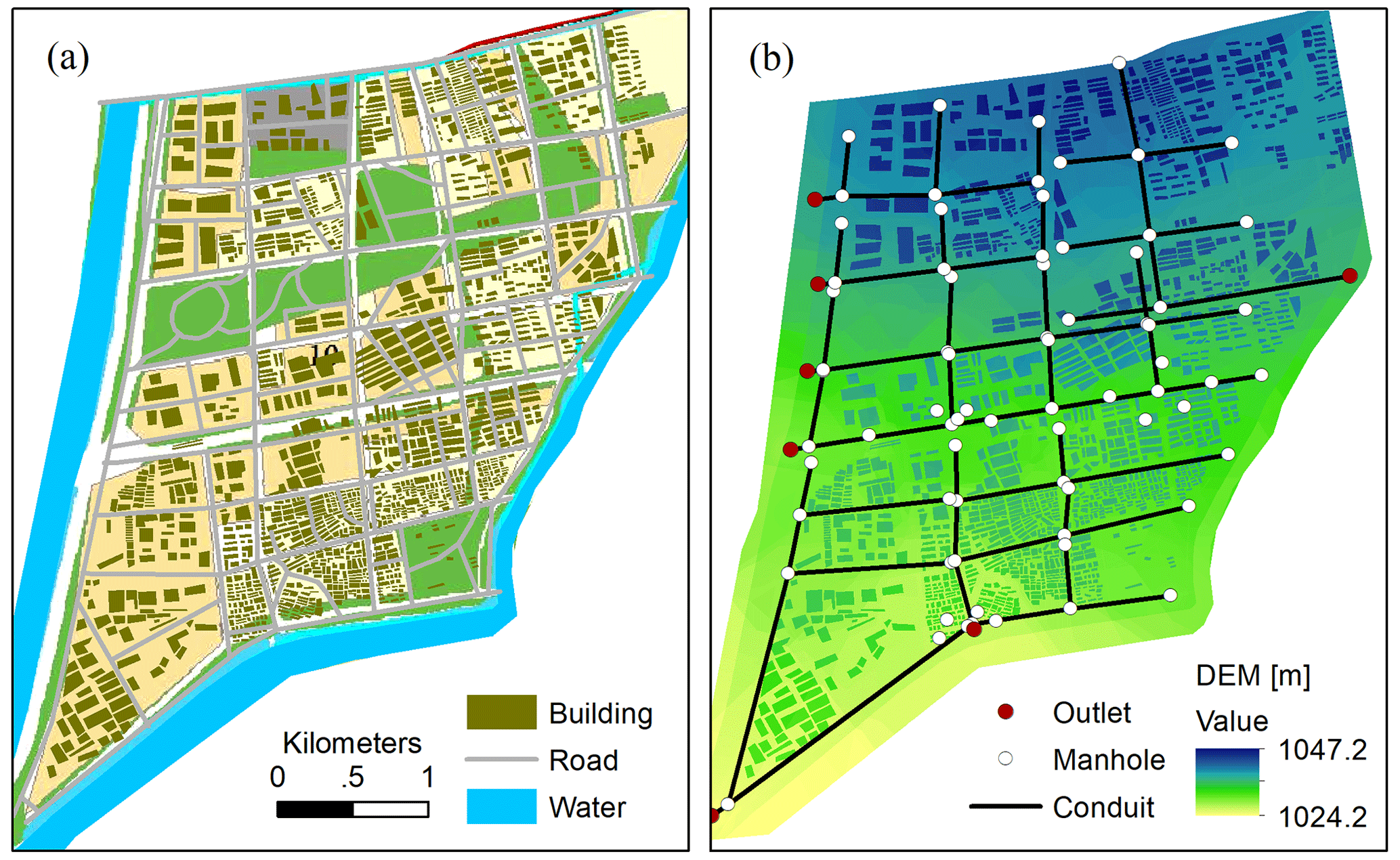
Figure 2(a) Land use and (b) drainage system and DEM of the second case study.
In this case study, we investigated the DL-based model ability for predicting both maximum water depth and flood time series during the entire rainfall period. Two types of datasets were established. The first is (1) the maxH dataset, i.e., the maximum flood depth. There were in total 90 rainfall events adopted, with return periods ranging from 1 to 100 years and a rainfall duration of 2, 4, or 6 h, respectively. Meanwhile, three types of rain peak position coefficients were tested, including 0.3, 0.5, and 0.7. All rainfall inputs were generated with a temporal resolution of 10 min. The details on the return period, rainfall duration, and peak position of the input rainfall events are provided in the Supplement (Sect. S1). Among the 90 flood maps, 90 % were randomly selected for model training and validation, and the rest 10 % were for testing. The second is the (2) time series dataset. We adopted 11 rainfall events and recorded the flooded water depths every 10 min for the entire case study under each rainfall period. Among those chosen, nine rainfall events were used for training and the other two for testing. Furthermore, a second study was adopted to test the capability of the developed model to generalize to different case studies or contexts. The area is in a relatively remote location in the Hohhot city, and Fig. 2 shows the main land use, drainage system, and surface elevation of the case study. In this case study, the DL-based model was mainly tested on the basis of maxH predictions.
2.2 Physically based hydrodynamic model
All the overland flooding maps and time series were simulated using the 1D–2D coupled hydrodynamic model, namely MIKE URBAN (Mike by Dhi, 2016). The hydrological inputs and pipe flows were simulated using the 1D MOUSE model, and the overland flows were calculated using the MIKE 21 model. With the precipitation inputs, the runoff model was characterized by the general catchment data, such as locations, areas, imperviousness, and time of concentration. The shape of the runoff hydrograph was computed by the time–area method (Mike by Dhi, 2016). The calculation of unsteady flow in the pipe network was conducted by solving the Saint–Venant equations, which are the vertically integrated equations for the conservation of continuity (i.e., continuity equation) and momentum (i.e., momentum equation). The surface inundation model was established by the MIKE 21 rectangular grid component, and the links between the 1D and 2D models were established to simulate the flow interactions between the pipeline and overland flows. The flow in the links was governed by an orifice equation (Mike by Dhi, 2016). When the underground drainage was surcharged, the excess water flowed to the surface and conducted surface inundation calculations in the context of extreme precipitation. On the surface, the water typically flowed along buildings or streets based, on a description of the local digital elevation or topography (Mark et al., 2004; Leandro et al., 2009).
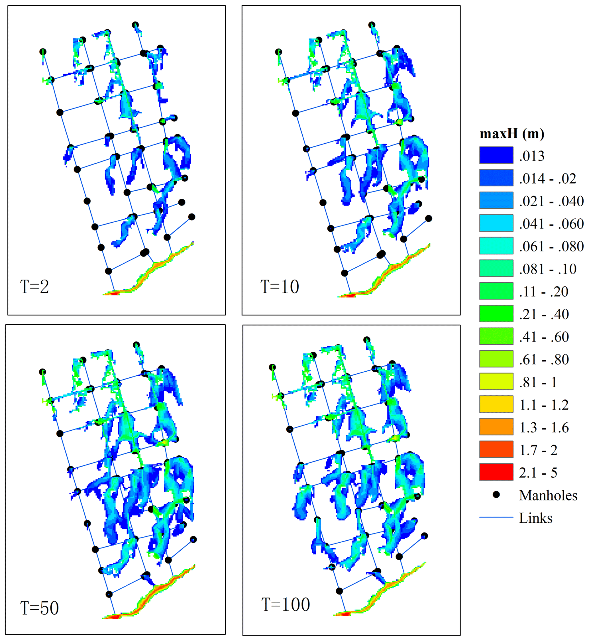
Figure 3Maximum flood maps simulated using the hydrodynamic model for four types of return periods. The unit of T is given in years.
The model outputs include the overland flow paths, extents, depths, and velocities at different time steps. One of the most commonly used outputs is flood maps describing the maximum water depths caused by the given rainfall inputs (Kaspersen et al., 2017; Mike by Dhi, 2016; Zhou et al., 2012). These flood maps can be further integrated with vulnerability data for an assessment of flood risk levels at different spatial scales (Sampson et al., 2014; de Moel et al., 2009; Ashley et al., 2007). In doing so, the critical areas with higher levels of flood risks can be identified and allocated with varying degrees of priority in the mitigation and adaptation plans (de Moel et al., 2015; Zhou et al., 2012). Taking the first case study as an example, as shown in Fig. 3, changes in input rainfalls lead to variations in the simulated flood maps. Increases in flood extents and depths are seen with rainfall that has larger return periods. Note that this study aimed to develop a flood prediction model that is applicable to various types of case studies and is not just intended to be a surrogate model of the physical model. The physical model was used to provide training samples for the DL model to learn the flood feature extraction ability. That means that all the tested hyetographs were the inputs and all the simulated flood maps were the ground truth (GT) data to train the model network. After the training, the randomly sampled 10 % flood maps were used to test the model prediction performances.
2.3 Deep learning model for flood prediction
2.3.1 LSTM (long short-term memory) network
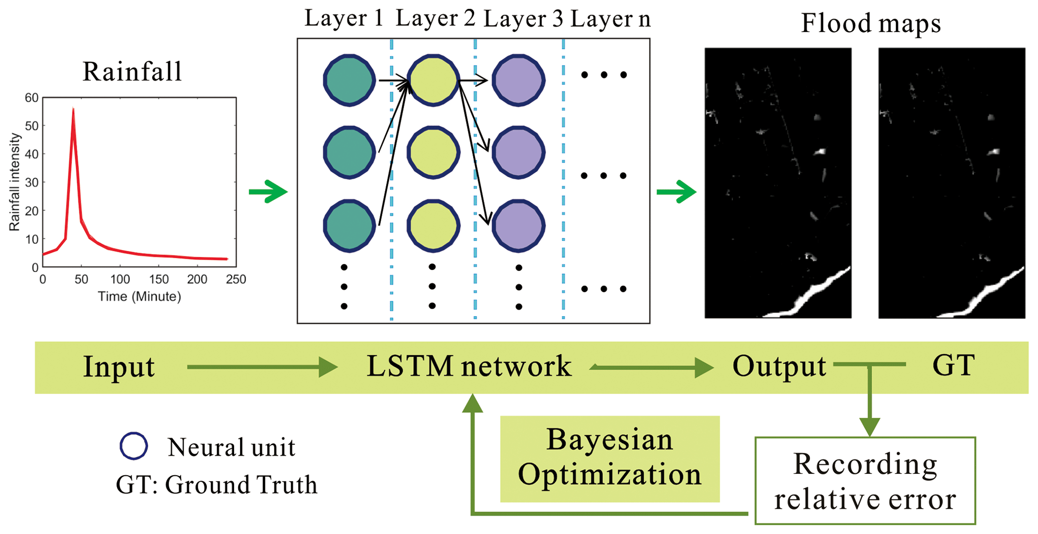
The LSTM network has advantages when processing time series data, especially for the long-term time-varying data. As shown in Fig. 4, the LSTM network is used to predict the flood maps. Ideally, the network can predict the flood depth distributions in the region as accurately as the real values/ground truth (GT) values can. The relative error between the output and GT values is calculated and used as an a priori condition for the Bayesian optimization (BO). This a priori probability is then used as the basis for selecting the network structure and hyperparameter combinations in the next iteration. Finally, an optimal network model (e.g., with an appropriate number of layers) and the corresponding hyperparameters are obtained through the iterative BO process.
The LSTM network requires only rainfall intensity as the input, and the output is the water depth of all grid points all at once. That means that LSTM outputs a 2D map directly, which describes the water depth of the entire site. A regression algorithm is used for the LSTM model. Specifically, the input rainfall intensity is processed through multiple LSTM layers and activation layers, and finally, a regression layer outputs the water depth of all grid points. In other words, the process is akin to a fitting process in which different rainfall intensities are matched nonlinearly to the water depth of the grid points. The number of output grids can be set during LSTM modeling so that the output grid can be specified for different sites.
It is noted that the terrain feature (e.g., digital elevation model or DEM) is a key factor in implementing flood prediction tasks. Besides, catchment hydrological properties (e.g., land use, area, and imperviousness) and network parameters (pipeline distribution and capacity) also have essential impacts on flood conditions. When designing the method, we considered the impacts of all influencing factors in the network training but without specifying/demanding them in the model input. There are two main reasons. (1) The site information contains a vast amount of data. Although computer technology has made significant progress, DL algorithms still face significant challenges in processing high-dimensional data. Such data can significantly decrease the prediction efficiency, particularly when applied to large-scale areas. The method proposed mitigates the impacts of the high-dimensional sites' data on the prediction efficiency. (2) Neural network technology involves learning and creating a mapped relationship between the input and output data. The function of the LSTM model is to establish the nonlinear mapping relationships between the input rainfall intensity, the implicit influence conditions, and the output flood depth to reflect the impact of these factors.
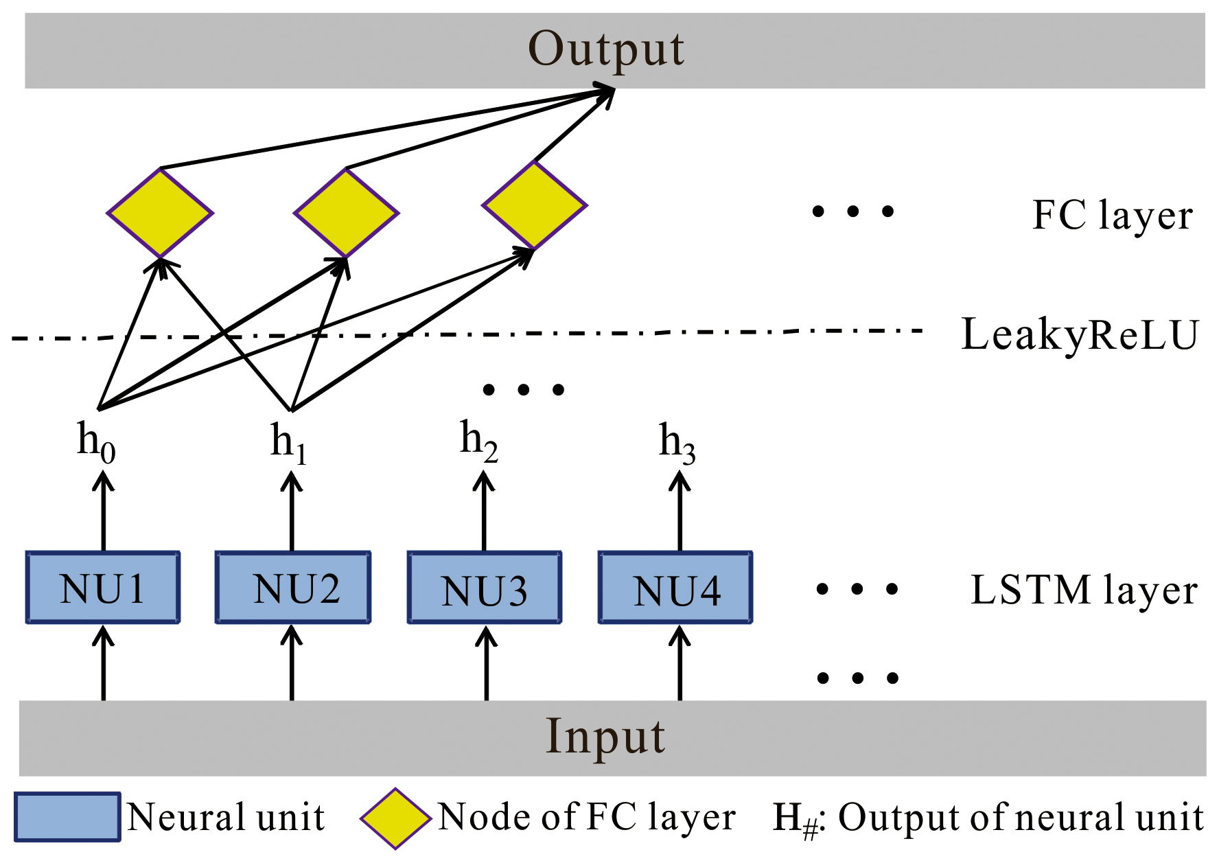
A benchmark LSTM network structure is shown in Fig. 5. With the input data (rainfall intensity), the LSTM obtains the output (water depth) through a series of functional layers, including a LSTM layer (containing N neural units), a Leaky rectified linear unit (ReLU) activation function (Eq. 1), and a fully connected (FC) layer. In the LSTM layer, the rainfall is input to the N neural units to obtain the N outputs (i.e., h0, h1, h2,…, hN). The outputs of these neural units are then transformed nonlinearly by the Leaky ReLU activation function and enter the FC layer. Eventually, the FC layer delivers the output of the network. Specifically, the LSTM network is trained through the adaptive moment estimation (Adam) optimizer (Eqs. 2–4). Meanwhile, two performance indicators are used to reflect the network training, which are the loss (Eq. 5) and root mean square error (RMSE; Eq. 6), respectively.
where x and scale are the input and scale factor (0.01), receptively. Any input value that is less than zero is multiplied by a fixed-scale factor. β1 and β2 are the gradient decay factor (0.9) and squared gradient decay factor (0.999), respectively. E(θ) is the loss function, m and v are the momentum terms, and ε = 10−8. n is the number of samples, and yi and are the predicted and real results, respectively.
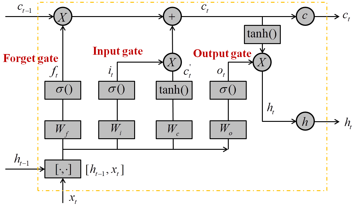
The neural unit is a key component of the LSTM network, and the structure of a single neural unit is shown in Fig. 6, including a forget gate (Eq. 7), an input gate (Eqs. 8–10), and an output gate (Eqs. 11 and 12). The forget gate determines how many unit states are retained from time (t−1) until time (t). The input gate determines the update of the unit states. The output of the LSTM neural unit state is determined by the nonlinear activation function (sigmoid in Eq. 13) and the output gate. In general, an input (x) passes through a neural unit to obtain an output (h). Specifically, the calculation process of a single LSTM neural unit is shown as follows:
where ft is the output of the forget gate, Wf and bf are the weight matrix and bias of the forget gate, and ht−1 and xt are the output of the previous neural unit (time t−1) and the current input (time t), respectively. it is the output of the input gate, and and ct are the unit state of the current input and current time, respectively. ot is the output of the output gate, and ht is the neural unit output of time (t).
In this paper, the LSTM network was built in the MATLAB 2021a (MathWorks Inc, Natick, MA, US). The input was the rainfall intensity varying with time, and the output was the maxH flood maps or water depths at different time steps of the case study sites. The training platform was performed on a computer with an NVIDIA GeForce RTX 2060 GPU, using an Intel Core i7-4790 at 3.60 GHz CPU for Windows 10.
Furthermore, to validate the performance of the developed LSTM model, two additional baseline models were adopted for comparison, namely the artificial neural network (ANN) and the convolutional neural network (CNN). The ANN is a fully connected network (back-propagation neural network, BPNN) that included one input layer, one hidden layer (including 170 connection nodes/neurons), and one output layer. The ANN network has played an important role in the early research of artificial intelligence (Sudheer et al., 2002), as it has performed well in certain simple regression tasks. However, the fully connected structure has significantly increased the computing cost of the network and limited its further application in the big data field. On the other hand, the CNN network adopted included two convolution layers, one pooling layer, two activation layers, and a fully connection layer. The CNN has significantly reduced the network computing cost through weight sharing and the sparse connection. It has a strong feature extraction capability (Hinton and Salakhutdinov, 2006) and showed a stronger performance than the BPNN in related research (Teng et al., 2022). In this paper, we compared the classic and popular ANN and CNN as baseline networks with the developed LSTM to clarify the effectiveness and novelty of the method proposed.
2.3.2 Bayesian optimization
One problem with the aforementioned LSTM network is that its structure layers, learning rate, number of training epochs, mini-batch size, and number of neural units were all unknown. When starting from scratch, it can be very difficult and time-consuming to manually select and fine-tune these hyperparameters. Bayesian optimization (BO) is an algorithm that can automatically search for the optimal hyperparameter combinations. The BO is a continuously updated probability model (Eq. 14) and assumes that the probability of occurrence of Event A under the a priori condition of Event B is directly proportional to the probability of occurrence of the a posteriori condition of Event B. That is, for successively occurring events, the latter events are related to all previous events. It is a potential hyperparametric optimization scheme, which means that the most likely parametric combination is inferred through a number of a priori attempts (i.e., training network models with different structures).
The posterior probability of the optimization function is updated through a number of evaluations of the objective function to obtain the optimal parameter combination. It can provide a reference for the subsequent models tried, according to the a priori conditions (i.e., historical evaluation records, which are the mean relative errors in the tried network model in this paper). When selecting the next group of parameter combinations, the algorithm made full use of the previous evaluation information to reduce the search time of the parameters. Specifically, we designed a variety of search ranges of the hyperparameters, and the BO algorithm automatically took the values from the search ranges, constantly tried the network models with different structures, and then recorded the errors. In this paper, the hyperparameters to be optimized included the number of LSTM layer,learning rate, epoch, mini-batch size, and number of hidden units. The search ranges of these five parameters were set to [1–5], [10−4–1], [0–600], [0–100], and [0–100], respectively. Finally, BO inferred the possible optimal network combination according to the historical error information. The selection process is shown in Eq. (15).
where P(A|B) and P(A) are the posterior and prior probabilities of Event A, respectively, and P(B|A) is the observation point probability obtained from the previous events. f(x) is the objective function (i.e., the mean relative error (Eq. 16); see the next section), x∗ is the optimal parametric combination, and χ is the value range of parameters.
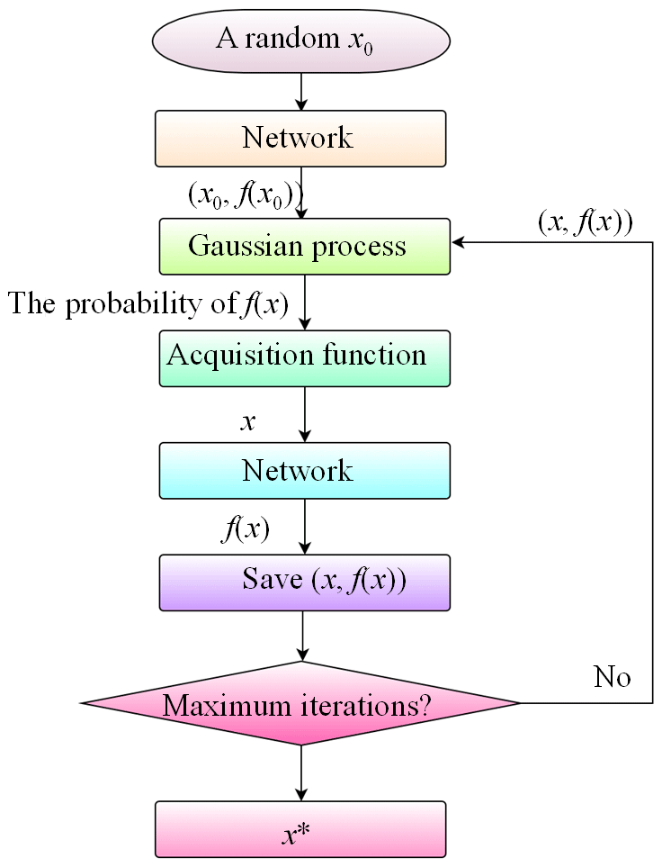
Specifically, the optimization workflow with regard to deep learning model is implemented, following Fig. 7. (1) A group with a hyperparameter combination x0 (e.g., MaxEpochs and learning rates) is randomly selected within the value ranges of the hyperparameters. (2) The x0 is input to the network for training to obtain the corresponding objective function f(x0). (3) The probability distribution of f(x) corresponding to x is calculated and predicted through the Gaussian process using all the inputs (x,f(x)). (4) The optimal x is determined by the acquisition function in the probability distribution. (5) The x obtained from step (4) is taken as the hyperparameter combination of the network to train and calculate the objective function f(x). (6) Before reaching the maximum iteration number, the (x,f(x)) obtained in step (5) is used as the input of the Gaussian process to continuously update the probability model to obtain a new (x,f(x)). Once the maximum iteration number is reached, the x corresponding to the minimum value of f(x) is taken as the optimal hyperparameter combination x∗.
2.3.3 Transfer learning (TL)
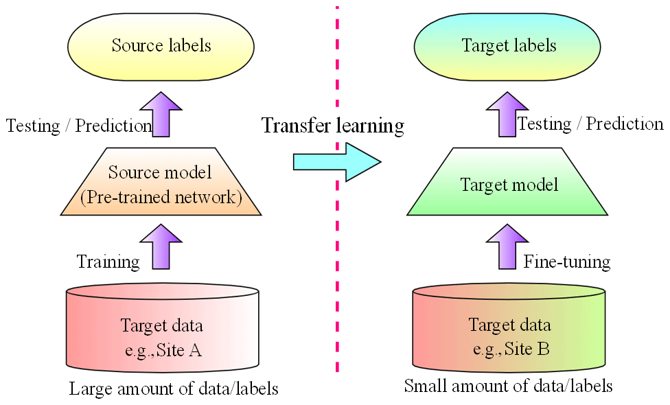
One of the main challenges of data-driven models is their compatibility, as it appears that, in this study, the model established is only applicable to the investigated site. This problem can be solved by using transfer learning (TL) technology to implement flood prediction for new sites. The TL, namely to learn from experience, can significantly improve the application field of intelligent algorithms. The TL is a DL method to transfer the knowledge from one domain (source domain) to another domain (target domain; see Fig. 8). Through the training of a source model (pre-trained network) using the source data (Site A), the pre-trained network can gain a strong ability of feature extraction in the similar tasks. Subsequently, with the fine-tuning (transfer learning) of the new data (Site B), the pre-trained network can quickly adapt to the new site under different scenarios. With this method, a lot of training time can be saved for the target domain (the new site), and better training effects can be achieved, especially when there are limited training samples in the target domain. In this paper, we used TL to transfer the LSTM network obtained from the current site (Site A) to the second case study site (Site B) with data from the new site, so as to expand the compatibility and generalization ability of the proposed method.
2.3.4 Performance indicators
In order to evaluate the reliability of the proposed method, five indicators were employed to evaluate the prediction results, focusing on estimating the differences in flood depths and the spatial patterns of the flood distributions. First of all, the mean relative error (Mre) was used to calculate the depth error between the prediction results (PR) and the ground truths (GT). Next, the 2-D correlation coefficient (2D-CC) and structural similarity (SS) were used to evaluate the correlation and similarity of images (distributions of flood areas), respectively. The Bhattacharyya distance (BD) and histogram intersection distance (HID) measure the similarity of two discrete or continuous probability distributions. They were adopted to evaluate the amount of overlap between two statistical samples or images (i.e., flood maps).
where and are the average pixel values of images I and J, respectively, μI, μJ, σI, σJ, and σIJ are the pixel local mean, standard deviation, and cross covariance of images I and J, respectively. C1 and C2 were 6.5 and 58.5, respectively. p(x) and q(x) are the probability distributions of pixels of Images I and J, respectively. X is the domain of p(x) and q(x).
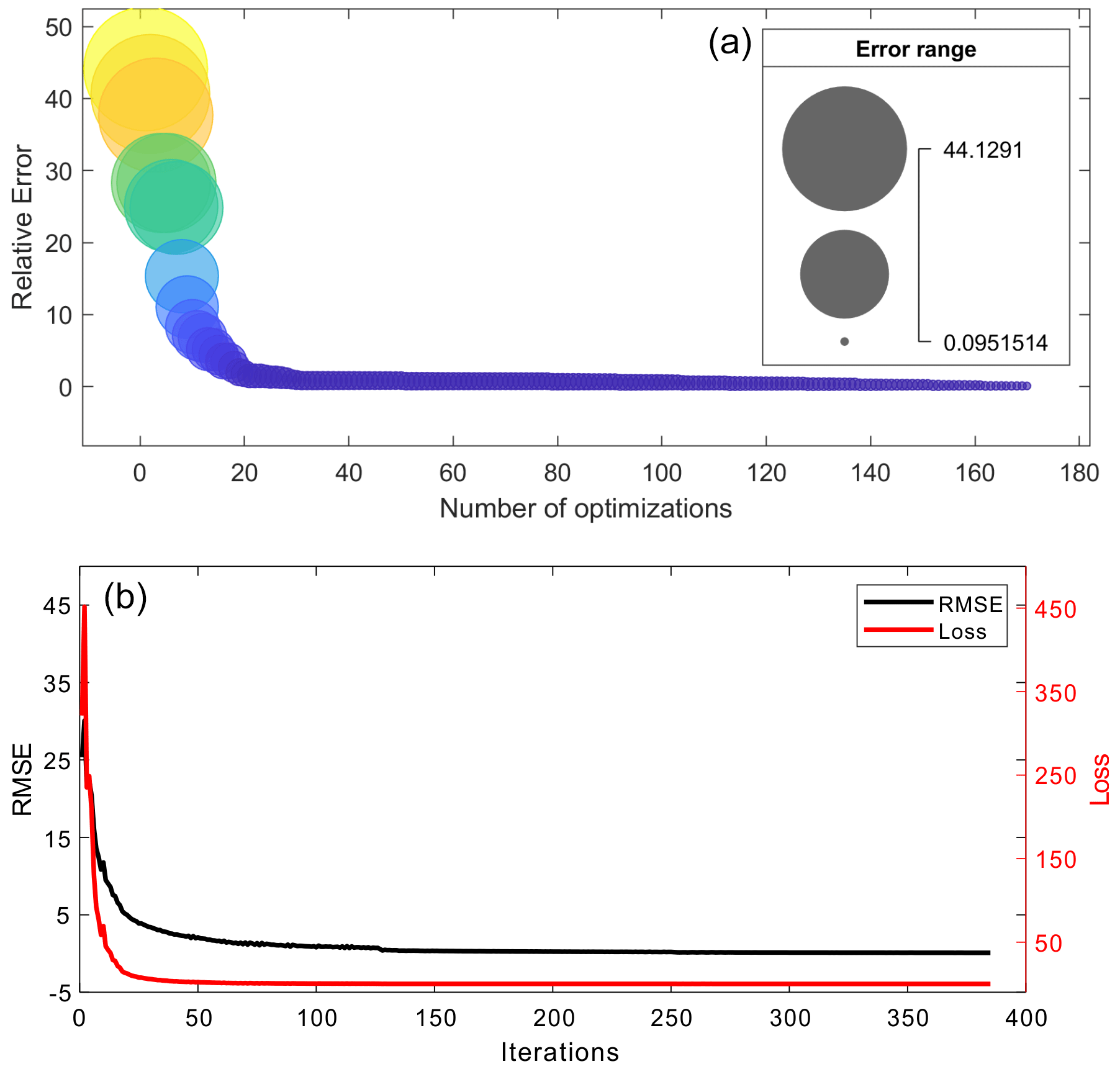
Figure 9(a) Mean relative errors along with the Bayesian optimization process and (b) the RMSE and loss achieved by the model with the best performance.
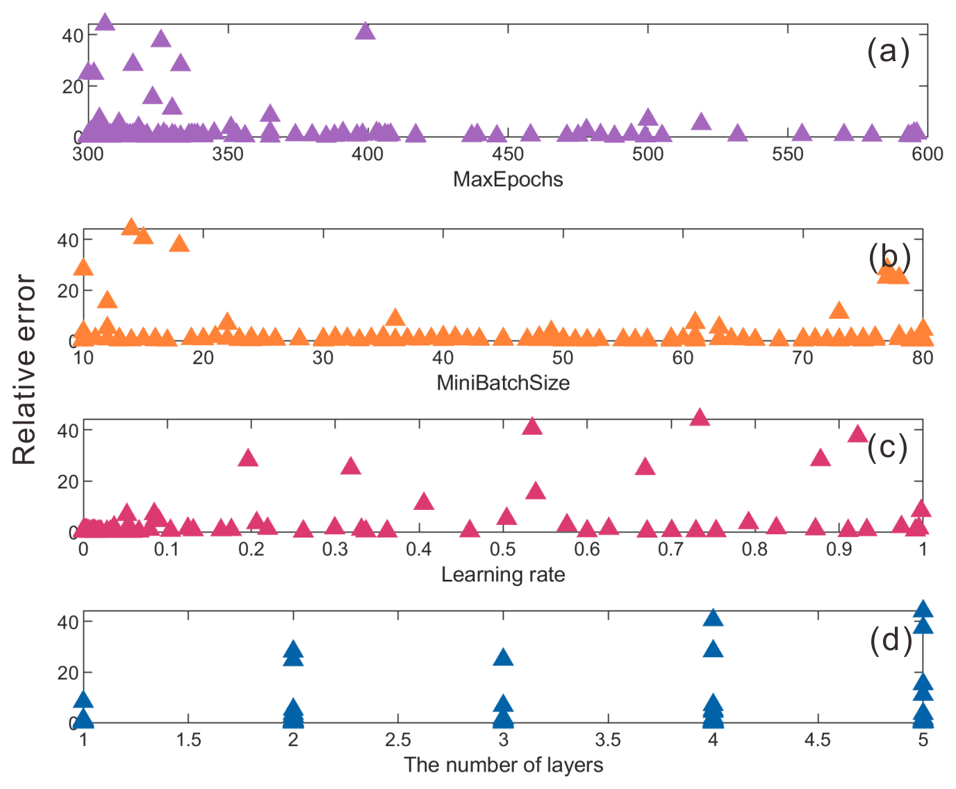

Figure 11The optimized model structure of the LSTM network. Batchnorm_# is the batch normalization layer that will normalize the network training data (mapping raw data to [0, 1]) and increase the training speed.
An illustration of the mean relative error in the testing dataset obtained from the 170 Bayesian optimizations is shown in Fig. 9a. The range of the mean error is between 0.095 and 44.13, and the size and color of the bubble chart represents the value of the mean error. It is clear that the error gradually decreased along with the iteration thanks to the optimization process. One of the networks, with a mean relative error value of 0.095, worked best in learning the flood map features. Figure 9b shows the RMSE and loss of the model accuracy, with the best performance identified from the Bayesian optimization. It is shown that the loss curve stably decreased along the network training and the model achieved a convergence status after the 100 iterations, with a small loss value. This implies that the DL network is very robust and trained well with the input data.
We further analyzed the influence of network parameters on the prediction results (Fig. 10). The results show the following. (1) There were large errors when the values of the MaxEpochs (i.e., maximum number of epochs) were set too low. Increasing the number of training epochs could avoid adverse events. (2) The MiniBatchSize had little influence on the prediction results, but it was not appropriate to take too large or small values. In this case, the MiniBatchSize of 20–70 could ensure an ideal prediction effect. (3) It is recommended to set a low learning rate. When the value was low, the achieved error was small and close to 0. (4) A deeper network layer could obtain a smaller prediction error. With the parameterization analysis, the best design scheme (network structure and hyperparameters) of the LSTM can be determined through the Bayesian optimization. The detailed network structure is shown in Fig. 11. The learning rate, MaxEpochs, MiniBatchSize, and number of hidden units were 0.0146, 385, 59, and 94, respectively.
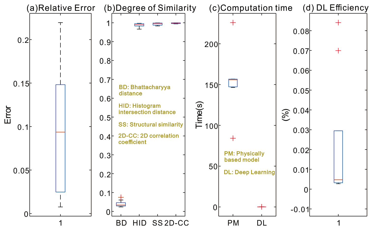
Figure 12(a) Relative error, (b) degree of similarity, (c) computation time, and (d) deep learning (DL) efficiency (i.e., computation time of DL model divided by computation time of hydrodynamic model) achieved with the testing datasets.
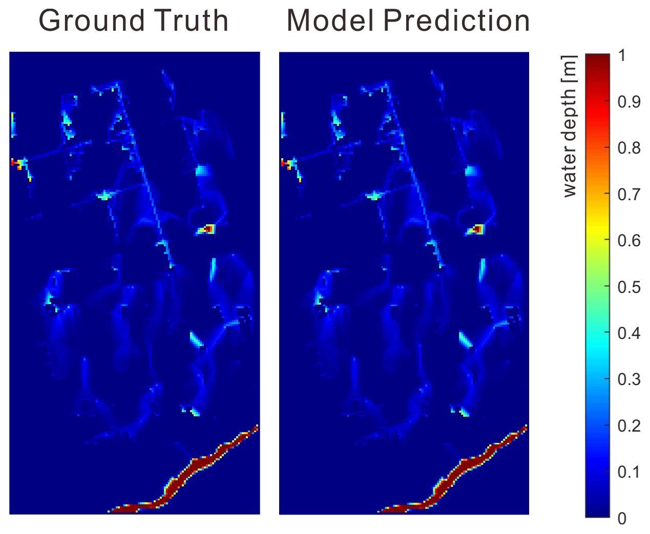
Figure 13Sample comparison of the flood maps between the ground truth and model prediction in the best-case scenario.

Figure 14Relative error in the (a) best- (i.e., minimum), (b) mean-, and (c) worst- (i.e., maximum) case scenarios, respectively. (d) Summary of the relative error data in box plots for the three types of scenarios.
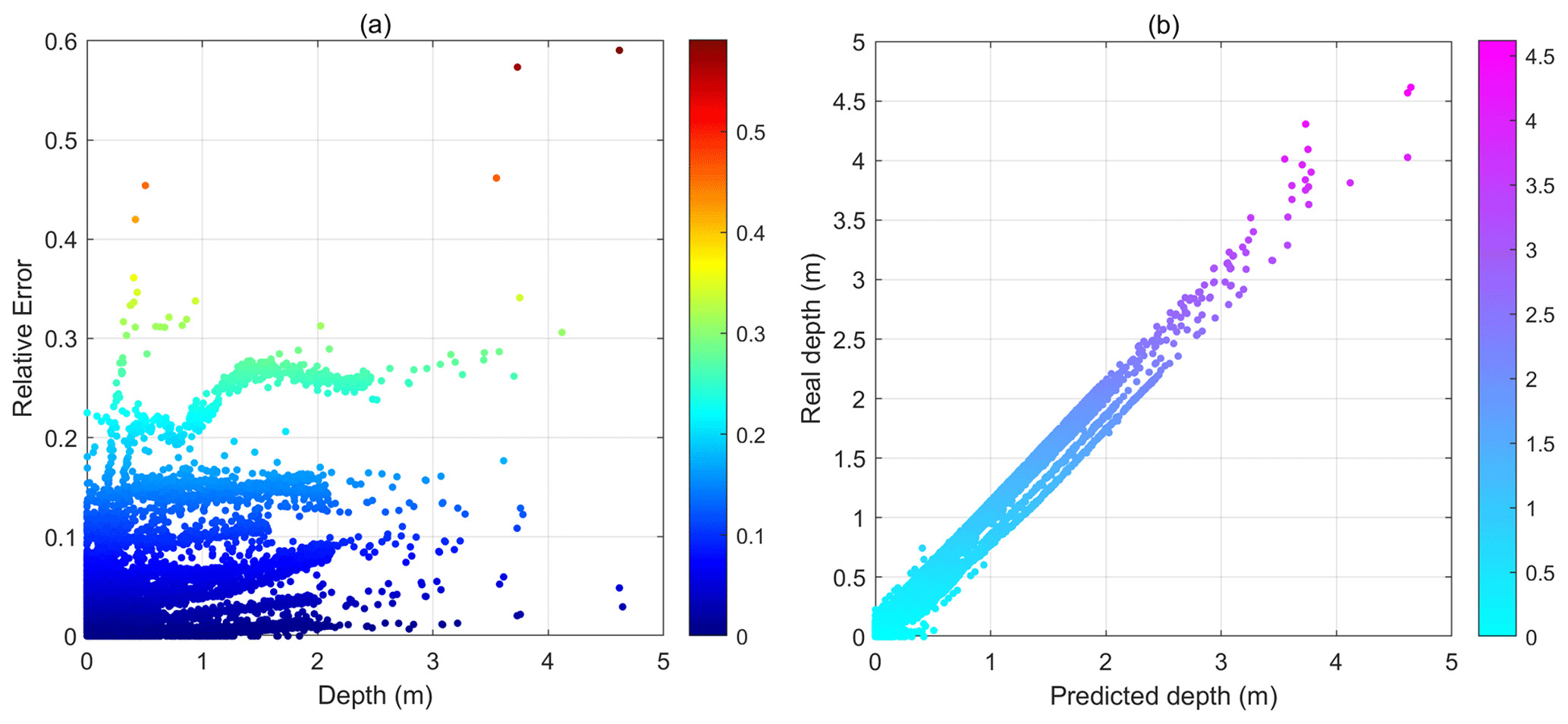
Figure 15(a) Relative errors in the predicted flood maps as a function of water depths and (b) ground truth water depths as a function of predicted water depths.
The statistics of the performance indicators of the best-performing model are analyzed in Fig. 12. First of all, the specific value of relative error in each testing flood map was summarized in the box plot in Fig. 12a. As reported previously, the LSTM model obtained satisfying results, with a mean relative error (RE) of 9.5 %. Among those results, the achieved minimum RE of a single prediction was only 0.76 %, which implies that the predicted flood map (both the inundation locations and depths) was very close to the ground truth map for validation. The degree of similarity is illustrated by the four types of indicators in Fig. 12b. The Bhattacharyya distances of the testing dataset were all close to zero, which meant that the spatial distributions of the ground truth and predicted flood hazard maps were very similar, and a majority of the two map populations overlapped. The ideal results were further validated by the histogram intersection distance, structural similarity, and 2D-CC, as their values were all close to 1. This implies that the spatial similarity of the predicted maps was very high. On the whole, the model proved to be superior in learning and predicting the flood maps with different hyetographs.
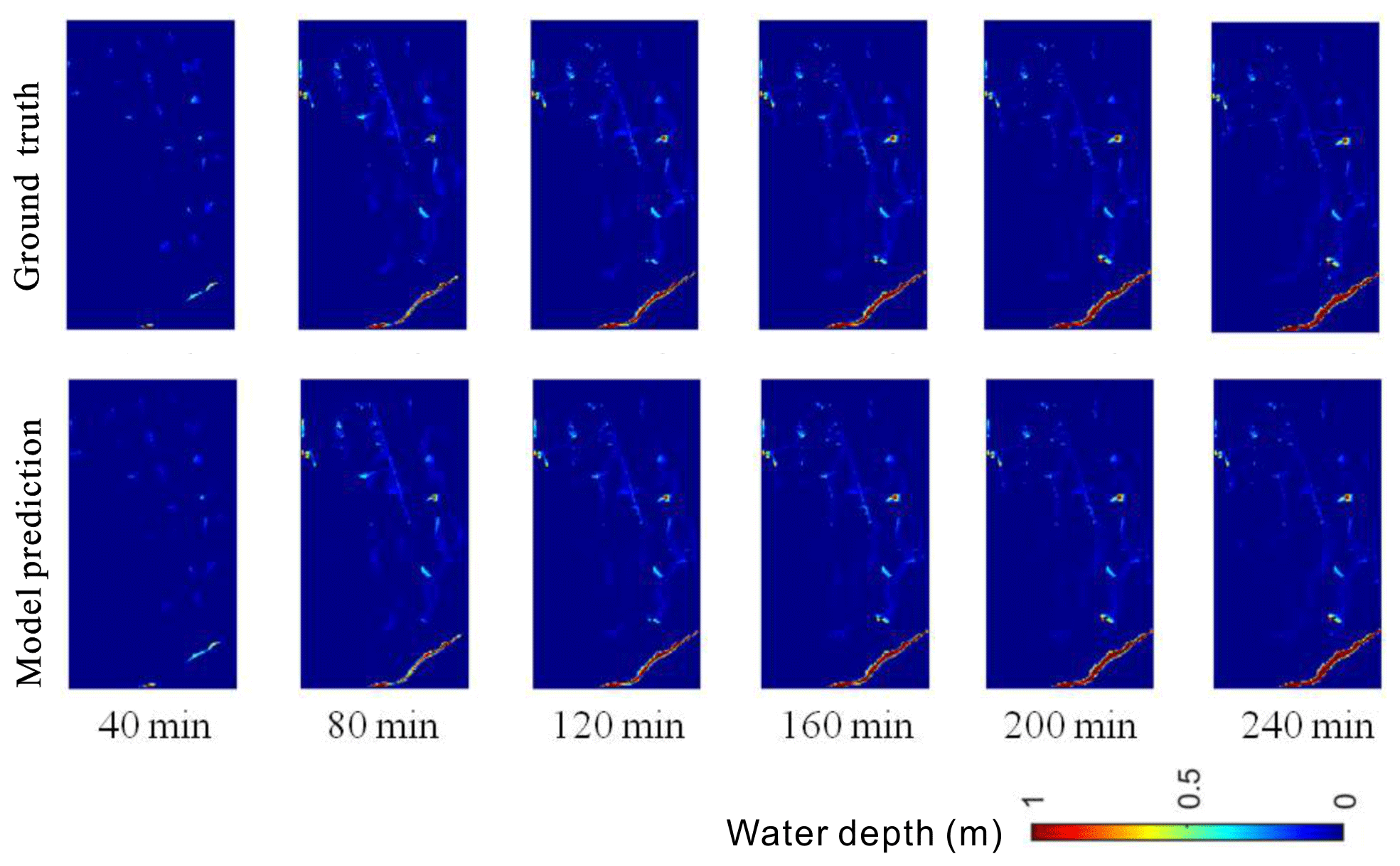
Figure 16Sample comparison of flood maps between ground truths and model predictions at different time steps in the first case study.
The computational times of the hydrodynamic model and the DL model are compared in Fig. 12c. The average computational time of the hydrodynamic model was 153.2 s, while the mean time of the prediction model was significantly reduced, with a value of 0.038 s. It is shown in Fig. 12d that the hydrodynamic model took almost 19 585 times (i.e., mean value) the simulation time of the DL model. In the worst case, the hydrodynamic model simulated the flood map more than 36 600 times slower. Note that the computation time of the hydrodynamic model was in fact even longer, as the model needed to run the hydrological and pipe network + 2-D simulations separately, and a manual integration of the two simulations was not taken into account. The results showed that, with proper model training, the LSTM model was accurate and much more computationally efficient, which can provide important support tools for real-time or rapid forecasting of urban flooding and emergency decision-making.
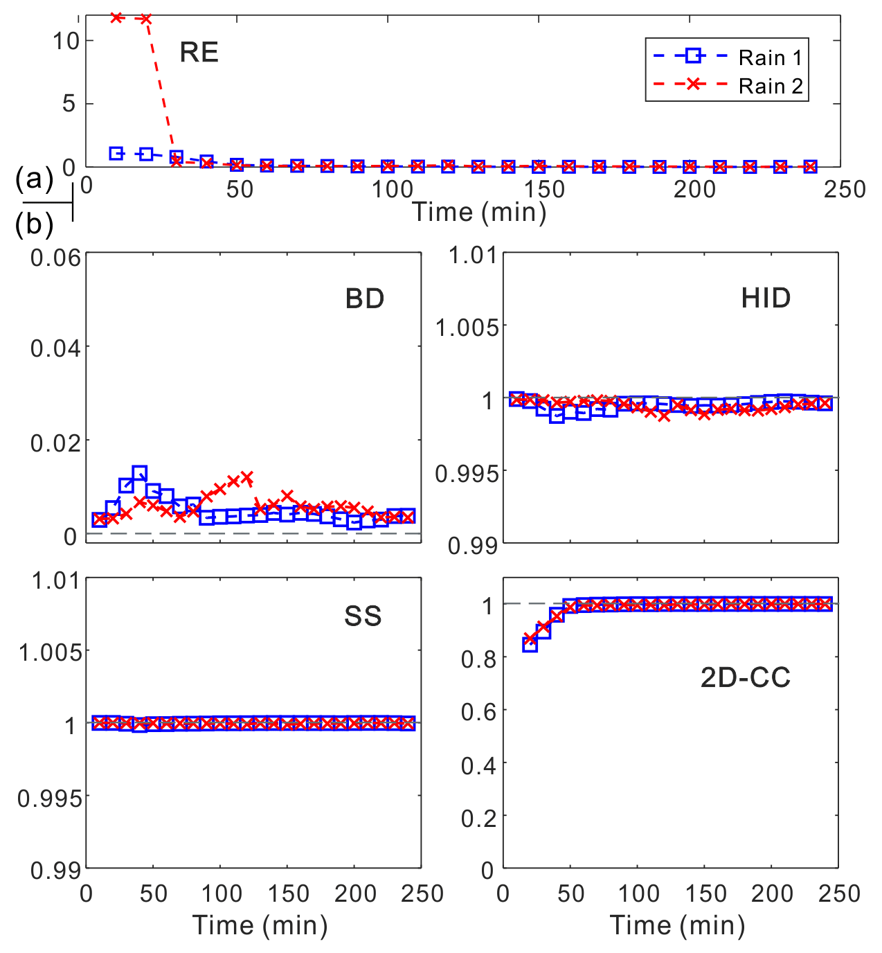
Figure 17(a) Relative error (RE) and (b) degree of similarity (BD, HID, SS, and 2D-CC) of the flood predictions when testing rainfall at different time steps.
Figure 13 illustrated the inundated areas of the ground truth and the predicted flood maps with the best model performance (i.e., with a minimum relative error). In total, there were 27 183 grids in each flood map. It is seen that the LSTM model successfully retrieved the depths and spatial patterns of the inundated areas. The two maps were almost identical, and it was very difficult to tell the difference without looking into further statistical details. Figure 14a shows the spatial distributions of the relative errors in the best-performing map. The differences between the two maps were almost negligible, except for the small regions near the waterbodies. The predicted flood map could identify all the flow paths and local depressions in the ground truth map. Moreover, the spatial distributions of the mean and maximum relative errors in the testing dataset are shown in Fig. 14b and c. Statistics (Fig. 14d) showed that, in all cases, the mean values were below 1 %, indicating a good agreement between the series of predictions and the ground truth maps. The errors were much higher in the worst case, where there were a small number of cells associated with relative errors greater than 20 %. Generally, the errors were greater where there were higher water depths and more flow volumes. Therefore, the high-error cells were mainly located in or near the waterbodies.
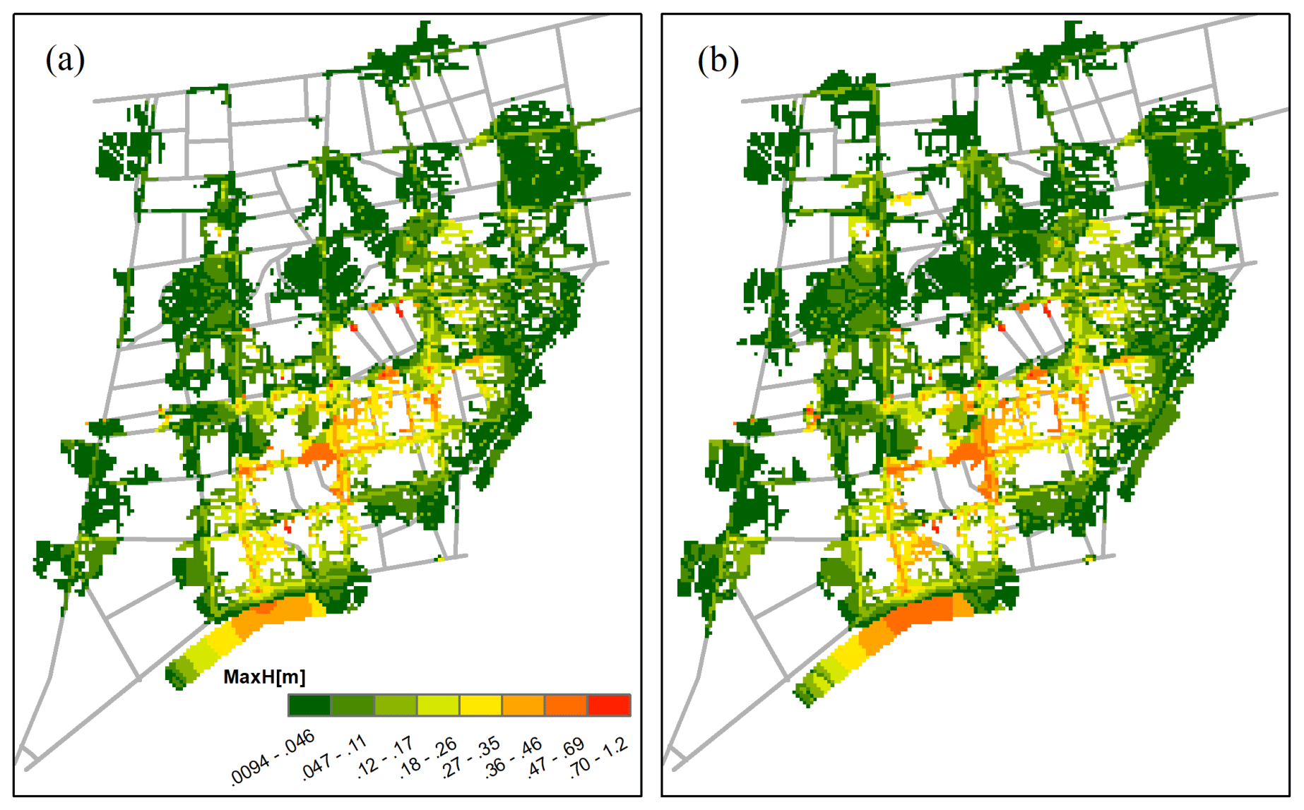
Figure 18Sample comparison of the flood map of the (a) ground truth and (b) model prediction in the second case study under a 50-year event.
The prediction accuracies of the deep learning model were further examined as a function of water depth in Fig. 15. Results show that the flood map dataset was imbalanced, as a majority of the results contain no and shallow water. Results show that, for water depths below 3 m, the model performed well, and most errors were below 2 %. The errors tended to increase under extreme conditions, with water depths above 3.5 m. Figure 15b shows that the predicted water depths are basically consistent with the ground truth water depths. These results clearly indicated that the deep learning model generalized well with the different hyetograph variations and could produce very accurate flood results, even with only rainfall inputs.
Figure 16 shows the sample comparison between ground truths and model predictions of flood maps in the time dimension. It was clear that our model could predict the flood variations at different time steps well. Following a visual inspection, the predicted flood maps were in a good agreement with ground truths at all time steps. The overall prediction effects (based on the relative error) and the evaluation indicators in terms of the degree of similarity are summarized in Fig. 17a and b for the time series predictions. Larger errors may occur in the early stage of rainfall, which could be due to the impacts of the drainage system on urban floods. Nevertheless, all the indicators further validated the model performance, which was also satisfying for predicting flood maps in that time dimension.
Table 1The performance indicators of the tested rainfall in the second case study.
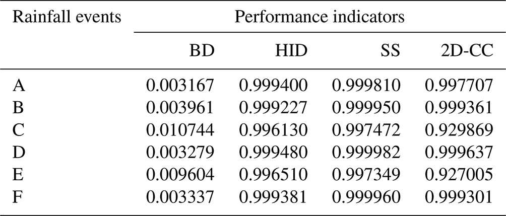
Figure 18 tested the performance of the established LSTM in the second case study. Results showed that, with transfer learning, the proposed model was applicable and generalizable to other cases, and the predicted flood maps were consistent and similar to the ground truths. Specifically, Table 1 shows the achieved performance indicators of all tested rainfall events. The obtained BD was close to 0, and HID, SS, and 2D-CC were close to 1, which meant that the model predictions were highly similar to the ground truth results. This proved that the flood prediction of the new site could be realized through transfer learning technology.
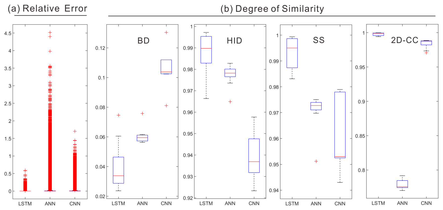
Figure 19(a) The mean relative error and (b) degree of similarity indicators of the proposed LSTM and two baseline models (ANN and CNN), respectively.
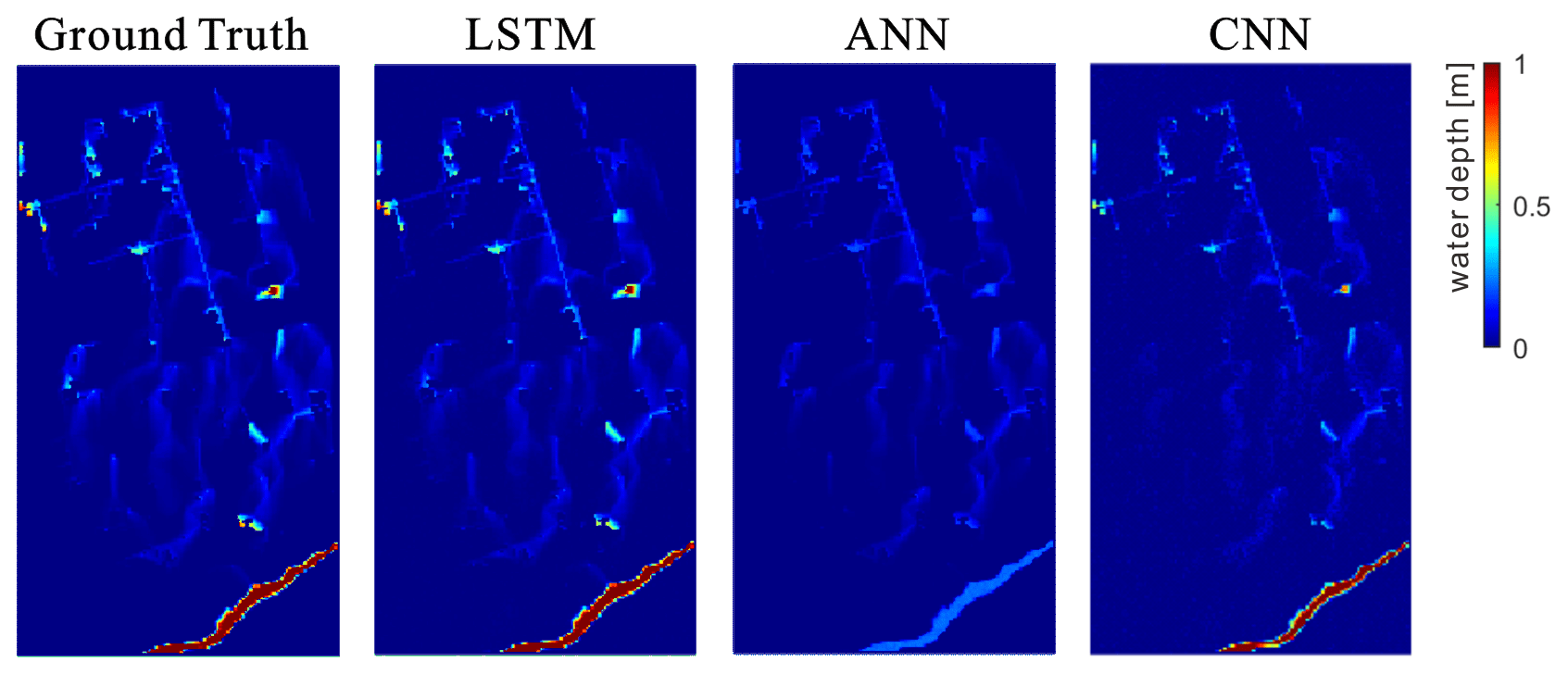
Figure 20A sample comparison of the flood inundation maps of ground truth, LSTM, ANN, and CNN models under an 85-year rainfall event.
Last, the proposed LSTM model was compared with the two baseline models (i.e., ANN and CNN) in Fig. 19. Our model outperformed the baseline models in terms of the evaluation indicators on both the relative error and the degree of similarity. This confirmed the excellent performance of LSTM in flood predictions for water depth and spatial distribution. The ANN performed poorly in predicting water depths, and there were a large number of cells associated with large errors. Regarding the BD, HID, and SS, the CNN was the least ideal for predicting the spatial distributions. One possible reason could be that the convolution operation of CNN filtered part of the feature information of the flood distribution. Note that the ANN's prediction based on the 2D-CC indicator was the worst. This could be due to fact that the fully connected network structure of ANN was prone to overfitting and may also have interference from some redundant information. Furthermore, a sample illustration of the predicted flood maps by the three types of models is shown in Fig. 20. It is clear that our proposed model was more competitive in flood predictions than the other two classical methods.
A rapid, accurate, and dynamic flood prediction tool is of great significance for urban water management to protect people, social assets, and the environment from flood hazards. This study proposed a DL-technique-based data-driven flood prediction approach, employing an integration of the LSTM technique, Bayesian optimization, and transfer learning approach. The results clearly showed that the model could accurately produce both the maximum water depths and the time series flood maps for various hyetograph inputs with much lower computational costs. Such types of predictions of dynamic changes on both the temporal and spatial scales are of great interest. By exploring the role of the Bayesian optimization algorithm in the LSTM network, the best design scheme of the network was determined. The results of our testing site showed that the LSTM could quickly adapt to the prediction task in the new site, and the transferred LSTM performed accurate flood predictions. The transfer learning method required less time, had lower resource costs, and delivered a better real-time performance, especially when dealing with large-scale site information.
The predicted flood maps were 19 585 times faster than the hydrodynamic model. The achieved mean relative error in water depths is 9.5 %, and the degree of similarity of the flood maps was very high. Specifically, in a best case, the difference between the ground truth and model prediction was only 0.76 %, and the spatial patterns of the two types of maps were almost identical. Meanwhile, the transfer learning technology has greatly improved the compatibility and generalization ability of the proposed method. The superior model performance was further validated by comparing it with the two baseline models. In conclusion, the accuracy and efficiency of the proposed method is satisfying.
We now acknowledge some limitations in this study and discuss directions of future work. First of all, the current training and testing data were obtained from hydrodynamic modeling due to a lack of detailed field site data. In future work, we consider adopting image-capturing techniques to supplement the data, such as DL techniques for the automated detection, acquisition, and evaluation of water depths from camera images. In doing so, there will be more real-case or field survey datasets for model training and testing. Meanwhile, the data augmentation is useful for enhancing the quantity and quality of input data, which will be tested in future investigations.
Despite these limitations, this work with its advances can contribute well to having a better understanding of the deep learning techniques for urban flood mapping. The proposed methodology predicts temporal and spatial water depths with only rainfall inputs and without further requirements of, e.g., local terrains and geographical conditions. The approach can be easily adjusted or adopted for other types of applications in the water management field. In summary, the method proposed represents a solution in the form of a compromise that takes into account prediction efficiency, accuracy, and adaptability. More importantly, the proposed method can potentially replace and/or complement the conventional detailed hydrodynamic model for urban flood assessment and management, particularly in applications of real-time control, optimization, and emergency design and planning.
The dataset that supports the findings of this study is available from the corresponding author upon reasonable request.
The supplement related to this article is available online at: https://doi.org/10.5194/hess-27-1791-2023-supplement.
QZ conceived the idea and acquired the financial support for the project. QZ and ST designed the study, conducted all the experiments, and analyzed the results. ZS, XL, and JF collected and preprocessed the data. QZ wrote the first draft, with contributions from ST and ZS. ZS, XL, JF, and GC provided feedback on the results and edited the paper. JZ and ZL provided the data and assisted with the analysis of the second case study and further improved the paper.
The contact author has declared that none of the authors has any competing interests.
Publisher's note: Copernicus Publications remains neutral with regard to jurisdictional claims in published maps and institutional affiliations.
This research has been funded by the Youth Promotion Program of the Natural Science Foundation of Guangdong Province, China (grant no. 2023A1515030126), the National Natural Science Foundation of China (grant no. 51809049), and the National College Students Innovation and Entrepreneurship Training Program (grant no. 202111845038).
This research has been supported by the Youth Promotion Program of the Natural Science Foundation of Guangdong Province, China (grant no. 2023A1515030126), the National Natural Science Foundation of China (grant no. 51809049), and the National College Students Innovation and Entrepreneurship Training Program (grant no. 202111845038).
This paper was edited by Dimitri Solomatine and reviewed by three anonymous referees.
Arnone, E., Pumo, D., Francipane, A., La Loggia, G., and Noto, L. V.: The role of urban growth, climate change, and their interplay in altering runoff extremes, Hydrol. Process., 32, 1755–1770, 2018.
Ashley, R., Garvin, S., Pasche, E., Vassilopoulos, A., and Zevenbergen, C.: Advances in Urban Flood Management, CRC Press, ISBN 978-0367389512, 2007.
Berggren, K., Packman, J., Ashley, R., and Viklander, M.: Climate changed rainfalls for urban drainage capacity assessment, Urban Water J., 11, 543–556, 2014.
Berkhahn, S., Fuchs, L., and Neuweiler, I.: An ensemble neural network model for real-time prediction of urban floods, J. Hydrol, 575, 743–754, 2019.
Ciechulski, T. and Osowski, S.: High Precision LSTM Model for Short-Time Load Forecasting in Power Systems, Energies, 14, 2983, https://doi.org/10.3390/en14112983, 2021.
Coulthard, T. J., Neal, J. C., Bates, P. D., Ramirez, J., de Almeida, G. A. M., and Hancock, G. R.: Integrating the LISFLOOD-FP 2D hydrodynamic model with the CAESAR model: implications for modelling landscape evolution, Earth Surf. Proc. Land., 38, 1897–1906, 2013.
Davidsen, S., Lowe, R., Thrysoe, C., and Arnbjerg-Nielsen, K.: Simplification of one-dimensional hydraulic networks by automated processes evaluated on 1D/2D deterministic flood models, J. Hydroinform., 19, 686–700, 2017.
de Moel, H., van Alphen, J., and Aerts, J. C. J. H.: Flood maps in Europe – methods, availability and use, Nat. Hazards Earth Syst. Sci., 9, 289–301, https://doi.org/10.5194/nhess-9-289-2009, 2009.
de Moel, H., Jongman, B., Kreibich, H., Merz, B., Penning-Rowsell, E., and Ward, P. J.: Flood risk assessments at different spatial scales, Mitig. Adapt. Strat. Gl., 20, 865–890, 2015.
Guo, Z., Leitão, J. P., Simões, N. E., and Moosavi, V.: Data-driven flood emulation: Speeding up urban flood predictions by deep convolutional neural networks, J. Flood Risk Manag., 14, e12684, 2021.
Han, H., Hou, J. M., Bai, G. G., Li, B. Y., Wang, T., Li, X., Gao, X. J., Su, F., Wang, Z. F., Liang, Q. H., and Gong, J. H.: A deep learning technique-based automatic monitoring method for experimental urban road inundation, J. Hydroinform., 23, 764–781, 2021.
Hinton, G. E. and Salakhutdinov, R. R.: Reducing the Dimensionality of Data with Neural Networks, Science, 313, 504–507, 2006.
Hofmann, J. and Schüttrumpf, H.: floodGAN: Using Deep Adversarial Learning to Predict Pluvial Flooding in Real Time, Water, 13, 2255, https://doi.org/10.3390/w13162255, 2021.
Hou, J., Zhou, N., Chen, G., Huang, M., and Bai, G.: Rapid forecasting of urban flood inundation using multiple machine learning models, Nat. Hazards, 108, 2335–2356, 2021a.
Hou, J. M., Ma, Y. Y., Wang, T., Li, B. Y., Li, X., Wang, F., Jin, S. L., and Ma, H. L.: A river channel terrain reconstruction method for flood simulations based on coarse DEMs, Environ. Modell. Softw., 140, 105035, https://doi.org/10.1016/j.envsoft.2021.105035, 2021b.
Hou, J. M., Li, X., Bai, G. G., Wang, X. H., Zhang, Z. X., Yang, L., Du, Y. E., Ma, Y. Y., Fu, D. Y., and Zhang, X. G.: A deep learning technique based flood propagation experiment, J. Flood Risk Manag., 14, e12718, https://doi.org/10.1111/jfr3.12718, 2021c.
Jamali, B., Löwe, R., Bach, P. M., Urich, C., Arnbjerg-Nielsen, K., and Deletic, A.: A rapid urban flood inundation and damage assessment model, J. Hydrol, 564, 1085–1098, 2018.
Skougaard Kaspersen, P., Høegh Ravn, N., Arnbjerg-Nielsen, K., Madsen, H., and Drews, M.: Comparison of the impacts of urban development and climate change on exposing European cities to pluvial flooding, Hydrol. Earth Syst. Sci., 21, 4131–4147, https://doi.org/10.5194/hess-21-4131-2017, 2017.
Leandro, J., Chen, A. S., Djordjevic, S., and Savic, D. A.: Comparison of 1D/1D and 1D/2D Coupled (Sewer/Surface) Hydraulic Models for Urban Flood Simulation, J. Hydraul Eng.-ASCE, 135, 495–504, 2009.
LeCun, Y. and Bengio, Y.: Convolutional networks for images, speech, and time series, in: The handbook of brain theory and neural networks, edited by: Arbib, M. A., MIT Press, 3361, https://doi.org/10.5555/303568.303704, 1995.
Li, W., Lin, K., Zhao, T., Lan, T., Chen, X., Du, H., and Chen, H.: Risk assessment and sensitivity analysis of flash floods in ungauged basins using coupled hydrologic and hydrodynamic models, J. Hydrol, 572, 108–120, 2019.
Lin, Q., Leandro, J., Wu, W., Bhola, P., and Disse, M.: Prediction of Maximum Flood Inundation Extents With Resilient Backpropagation Neural Network: Case Study of Kulmbach, Front. Earth Sci., 8, 332, https://doi.org/10.3389/feart.2020.00332, 2020.
Lowe, R., Urich, C., Domingo, N. S., Mark, O., Deletic, A., and Arnbjerg-Nielsen, K.: Assessment of urban pluvial flood risk and efficiency of adaptation options through simulations – A new generation of urban planning tools, J. Hydrol, 550, 355–367, 2017.
Löwe, R., Böhm, J., Jensen, D. G., Leandro, J., and Rasmussen, S. H.: U-FLOOD–topographic deep learning for predicting urban pluvial flood water depth, J. Hydrol, 603, 126898, https://doi.org/10.1016/j.jhydrol.2021.126898, 2021.
Mahmoud, S. H. and Gan, T. Y.: Urbanization and climate change implications in flood risk management: Developing an efficient decision support system for flood susceptibility mapping, Sci. Total Environ., 636, 152–167, 2018.
Mark, O., Weesakul, S., Apirumanekul, C., Aroonnet, S. B., and Djordjevic, S.: Potential and limitations of 1D modelling of urban flooding, J. Hydrol, 299, 284–299, 2004.
MIKE by DHI: MIKE by DHI software, Release Note_MIKE URBAN, 2016.
MOHURD: Technical Guidelines for Establishment of Intensity–Duration–Frequency Curve and Design Rainstorm Profile (In Chinese), Ministry of Housing and Urban-Rural Development of the People's Republic of China and China Meteorological Administration, ISBN 135029-5628, 2014.
MOHURD: Code for design of outdoor wastewater engineering (GB 50014—2006), Ministry Of Housing And Urban-Rural Development and Ministry Of National Quality Standard Monitoring Bureau, ISBN 915-5182074903, 2016 (in Chinese).
Moy de Vitry, M., Kramer, S., Wegner, J. D., and Leitão, J. P.: Scalable flood level trend monitoring with surveillance cameras using a deep convolutional neural network, Hydrol. Earth Syst. Sci., 23, 4621–4634, https://doi.org/10.5194/hess-23-4621-2019, 2019.
Panthou, G., Vischel, T., Lebel, T., Quantin, G., and Molinié, G.: Characterising the space–time structure of rainfall in the Sahel with a view to estimating IDAF curves, Hydrol. Earth Syst. Sci., 18, 5093–5107, https://doi.org/10.5194/hess-18-5093-2014, 2014.
Rawat, W. and Wang, Z.: Deep Convolutional Neural Networks for Image Classification: A Comprehensive Review, Neural Comput., 29, 2352–2449, 2017.
Sampson, C. C., Fewtrell, T. J., O'Loughlin, F., Pappenberger, F., Bates, P. B., Freer, J. E., and Cloke, H. L.: The impact of uncertain precipitation data on insurance loss estimates using a flood catastrophe model, Hydrol. Earth Syst. Sci., 18, 2305–2324, https://doi.org/10.5194/hess-18-2305-2014, 2014.
Sudheer, K. P., Gosain, A. K., and Ramasastri, K. S.: A data-driven algorithm for constructing artificial neural network rainfall-runoff models, Hydrol. Process., 16, 1325–1330, 2002.
Teng, S., Chen, G., Wang, S., Zhang, J., and Sun, X.: Digital image correlation-based structural state detection through deep learning, Frontiers of Structural and Civil Engineering, 16, 45–56, 2022.
Wang, N., Hou, J. M., Du, Y. G., Jing, H. X., Wang, T., Xia, J. Q., Gong, J. H., and Huang, M. S.: A dynamic, convenient and accurate method for assessing the flood risk of people and vehicle, Sci. Total Environ., 797, 149036, https://doi.org/10.1016/j.scitotenv.2021.149036, 2021.
Wolfs, V. and Willems, P.: A data driven approach using Takagi-Sugeno models for computationally efficient lumped floodplain modelling, J. Hydrol, 503, 222–232, 2013.
Wu, X., Wang, Z., Guo, S., Lai, C., and Chen, X.: A simplified approach for flood modeling in urban environments, Hydrol. Res., 49, 1804–1816, 2018.
Xia, D., Zhang, M., Yan, X., Bai, Y., Zheng, Y., Li, Y., and Li, H.: A distributed WND-LSTM model on MapReduce for short-term traffic flow prediction, Neural Comput. Appl., 33, 2393–2410, 2021.
Xie, K., Ozbay, K., Zhu, Y., and Yang, H.: Evacuation Zone Modeling under Climate Change: A Data-Driven Method, J. Infrastruct. Syst., 23, 04017013, https://doi.org/10.1061/(ASCE)IS.1943-555X.0000369, 2017.
Yin, D., Evans, B., Wang, Q., Chen, Z., Jia, H., Chen, A. S., Fu, G., Ahmad, S., and Leng, L.: Integrated 1D and 2D model for better assessing runoff quantity control of low impact development facilities on community scale, Sci. Total Environ., 720, 137630, https://doi.org/10.1016/j.scitotenv.2020.137630, 2020.
Yosinski, J., Clune, J., Bengio, Y., and Lipson, H.: How transferable are features in deep neural networks?, Proceedings of the Advances in Neural Information Processing Systems, Montreal, 8 December 2014, 3320–3328, 2014.
Zhang, B. and Guan, Y.: Watersupply & Drainage Design Handbook, China Construction Industry Press, Being, China, ISBN: 9787112136803, 2012.
Zhou, Q., Mikkelsen, P. S., Halsnaes, K., and Arnbjerg-Nielsen, K.: Framework for economic pluvial flood risk assessment considering climate change effects and adaptation benefits, J. Hydrol, 414, 539–549, 2012.
Zhou, Q., Ren, Y., Xu, M., Han, N., and Wang, H.: Adaptation to urbanization impacts on drainage in the city of Hohhot, China, Water Sci. Technol., 73, 167–175, 2016.
Zhou, Q., Leng, G., and Huang, M.: Impacts of future climate change on urban flood volumes in Hohhot in northern China: benefits of climate change mitigation and adaptations, Hydrol. Earth Syst. Sci., 22, 305–316, https://doi.org/10.5194/hess-22-305-2018, 2018.
Zhou, Q., Leng, G., Su, J., and Ren, Y.: Comparison of urbanization and climate change impacts on urban flood volumes: Importance of urban planning and drainage adaptation, Sci. Total Environ., 658, 24–33, 2019.
Zhu, S., Luo, X., Yuan, X., and Xu, Z.: An improved long short-term memory network for streamflow forecasting in the upper Yangtze River, Stoch. Env. Res. Risk A., 34, 1313–1329, 2020.
Ziliani, M. G., Ghostine, R., Ait-El-Fquih, B., McCabe, M. F., and Hoteit, I.: Enhanced flood forecasting through ensemble data assimilation and joint state-parameter estimation, J. Hydrol, 577, 123924, 2019.