Prediction of the absolute hydraulic conductivity function from soil water retention data

For modeling flow and transport processes in the soil–plant–atmosphere system, knowledge of the unsaturated hydraulic properties in functional form is mandatory. While much data are available for the water retention function, the hydraulic conductivity function often needs to be predicted. The classical approach is to predict the relative conductivity from the retention function and scale it with the measured saturated conductivity, K_s. In this paper we highlight the shortcomings of this approach, namely, that measured K_s values are often highly uncertain and biased, resulting in poor predictions of the unsaturated conductivity function.

We propose to reformulate the unsaturated hydraulic conductivity function by replacing the soil-specific K_s as a scaling factor with a generally applicable effective saturated tortuosity parameter τ_s and predicting total conductivity using only the water retention curve. Using four different unimodal expressions for the water retention curve, a soil-independent general value for τ_s was derived by fitting the new formulation to 12 data sets containing the relevant information. τ_s was found to be approximately 0.1.

Testing of the new prediction scheme with independent data showed a mean error between the fully predicted conductivity functions and measured data of less than half an order of magnitude. The new scheme can be used when insufficient or no conductivity data are available. The model also helps to predict the saturated conductivity of the soil matrix alone and thus to distinguish between the macropore conductivity and the soil matrix conductivity.

1 Introduction

Accurate representations of the soil hydraulic properties (SHPs) in functional form are essential for simulations of water, energy, and solute transport in the vadose zone. Classical models for the soil water retention curve (WRC) (e.g., van Genuchten, 1980; Kosugi, 1996) and the related hydraulic conductivity curve (HCC) derived using pore-bundle concepts (e.g., Burdine, 1953; Mualem, 1976a) account for water storage and flow in completely filled capillaries but neglect adsorption of water and water flow in films and corners. We will refer to the latter processes as “non-capillary” as opposed to “capillary” in the remainder of this article. In this paper, the term “non-capillary” is used only for water held by adsorption, although water in very large pores (i.e., larger than 0.3 mm in diameter; Jarvis, 2007) is also not held by capillary forces. The non-capillary parts of the WRC and HCC become dominant when soils become dry (Iden et al., 2021a, b). Therefore, improved models of the SHPs have been proposed that extend models that were established for the wet range towards the dry range (e.g., Tuller and Or, 2001; Peters and Durner, 2008a, Lebeau and Konrad, 2010; Zhang, 2011; Peters, 2013). In the very dry range, liquid flow ceases, and vapor flow becomes the dominant transport process. Isothermal diffusion of water vapor can be expressed in terms of an equivalent hydraulic conductivity and incorporated into an effective conductivity function (Peters, 2013). The total hydraulic conductivity can then be expressed as the sum of three components:

$$\begin{array}{}\text{(1)}& K\left(h\right)=K_{\mathrm{c}}\left(h\right)+K_{\mathrm{nc}}\left(h\right)+K_{\mathrm{v}}\left(h\right),\end{array}$$

where h [m] is the suction (i.e., the absolute value of the matric head or pressure head); K [m s⁻¹] is the total hydraulic conductivity; and K_c, K_nc, and K_v [m s⁻¹] are the hydraulic conductivity components for capillary and non-capillary flow of liquid water and water vapor diffusion in the soil gas phase, respectively. Under isothermal conditions, the function K_v(h) can be predicted easily from the temperature-dependent diffusion coefficient of water vapor in air and the WRC (Saito, 2006; Peters and Durner, 2010). Recently, Peters et al. (2021) combined the mechanistic models of Lebeau and Konrad (2010) and Tokunaga (2009) with the conceptual model of Peters (2013) to obtain a simple prediction scheme for the absolute non-capillary conductivity function K_nc(h).

Several models have been proposed to estimate the capillary conductivity function K_c(h) from conceptualizations of the pore space involving tortuous and interconnected pore bundles, most of which go back to the seminal studies by Burdine (1953) and Childs and Collis-George (1950) (CCG). Today, the capillary bundle model of Mualem (1976a), who refined the assumptions of the CCG model, is most frequently used (see Assouline and Or, 2013, for a critical review of this and similar models). The pore-size distribution of a porous medium is derived from the WRC, while the HCC is predicted using Poiseuille's law and some assumptions about the connectivity and tortuosity of the pore network. Attempts to predict the absolute capillary conductivity based on these theories (e.g., Millington and Quirk, 1961; Kunze et al., 1968) were not very satisfying because of large deviations with measured conductivities. However, the general shape of the HCC could be described well. Therefore, the models used in practice today predict a relative hydraulic conductivity function K_rc(h) and scale it by fitting the function to one or more measured conductivity points. Most commonly, the measured saturated conductivity is used for this purpose. A comprehensive overview of these models is given by Mualem (1986). More recently, concepts to predict the saturated hydraulic conductivity K_s [m s⁻¹] from the WRC were derived by Guarracino (2007), who used a fractal approach, and Mishra and Parker (1990) and Nasta et al. (2013), who used capillary bundle models to estimate K_s as a function of the WRC.

When predicting the hydraulic conductivity using a relative conductivity function that needs to be scaled by matching it to measured data, one faces three types of problems. First and most obviously, if no conductivity data are available for matching, scaling the relative conductivity is not possible. This is frequently the case. Second, if only measurements of K_s are available, the unsaturated conductivity estimates will be greatly affected by the dominant influence of structural pores on the variability of K_s. Thirdly, even if unsaturated conductivity data are available, the conductivity function near saturation may not be represented well. The latter two problems are outlined below.

The problem of scaling K_rc(h) by K_s stems from the influence of soil structure on the hydraulic conductivity at or near saturation. For more than 50 years, K_s has been known to vary over many orders of magnitude, even at the same site with a rather homogeneous texture (Nielsen et al., 1973; Kutílek and Nielsen, 1994, p. 249). If soil structure is not properly reflected in the WRC near full saturation, scaling K_rc(h) with a measured K_s can lead to severe overestimation of conductivity in the medium moisture range (Durner, 1992, 1994; Schaap and Leij, 2000). We exemplarily illustrate this problem in Fig. 1, top, for a sandy soil. The average difference between data and model in the unsaturated region in this example is about 1 order of magnitude.

A better choice is therefore to use unsaturated conductivity data to scale the relative conductivity curve, as already proposed by Nielsen et al. (1960). However, such data are often not available, especially if the measurements were made in the past when more recent techniques such as the simplified evaporation method (SEM) (Schindler, 1980; Peters and Durner, 2008b, Peters et al., 2015) were not available. Moreover, the SEM typically yields information only in a limited suction range, typically between h≈0.6 to h≈8 m, because of the limited measurement range of tensiometers and the fact that the highest measurable conductivity by SEM is of the same order of magnitude as the evaporation rate (i.e., between 10⁻⁸ and 10⁻⁷ m s⁻¹ depending on the laboratory conditions). This is particularly problematic with coarse materials for which the conductivity close to saturation is many orders of magnitude larger. We illustrate this problem in Fig. 1, bottom, which shows data for a well-graded sand, together with the fitted water retention and hydraulic functions. Whereas the match between model and the available data appears almost perfect, the conductivity curve near saturation is unreliable, and the model-predicted saturated conductivity of $\mathrm{1.7}\times {\mathrm{10}}^{-\mathrm{7}}$ m s⁻¹ (or 1.5 cm d⁻¹) is at least 2 orders of magnitude too low for such a soil.

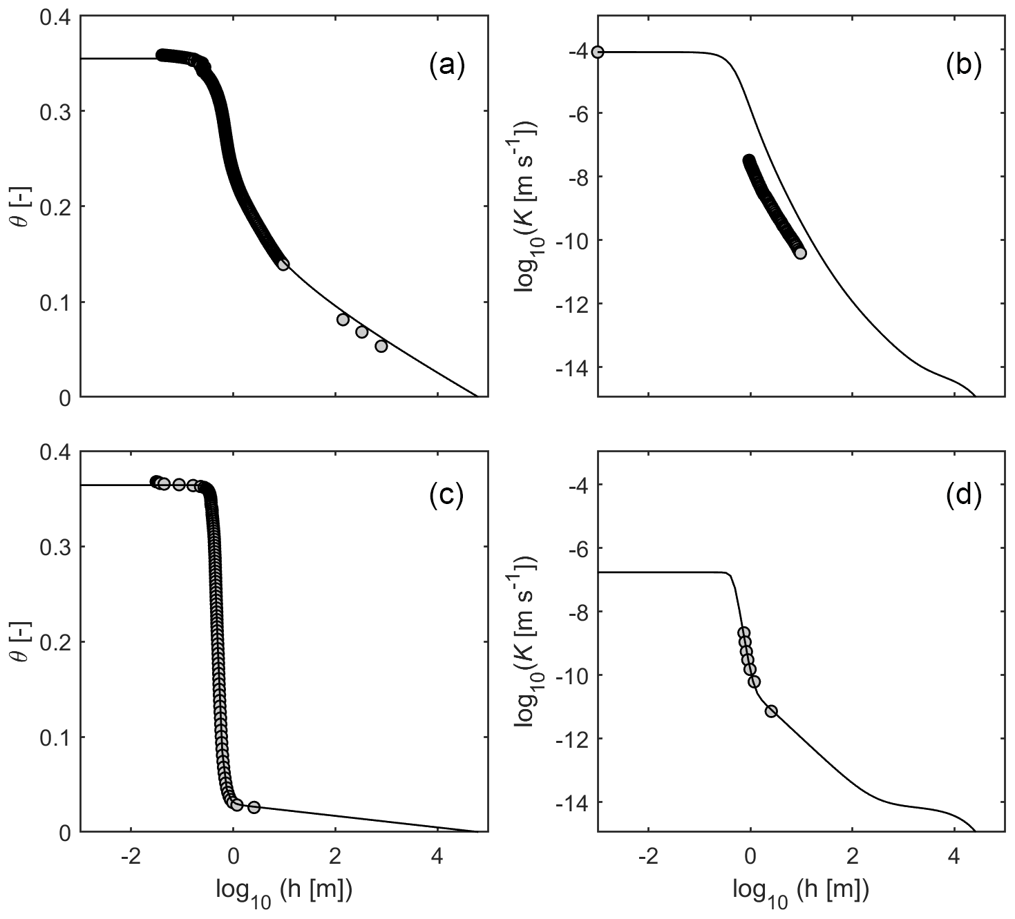
Figure 1 Example of conductivity predictions for two soils as obtained by scaling the capillary conductivity with measured conductivity data. Plots on the left side show fitted retention functions; plots on the right side show the corresponding predicted conductivity functions. (a, b) K prediction by matching the relative K function to the saturated conductivity, K_s. (c, d) K prediction by matching the relative K function to unsaturated conductivity data, obtained using the simplified evaporation method. The retention functions and corresponding predicted hydraulic conductivity functions were parameterized using the Peters–Durner–Iden model system with the basic van Genuchten saturation function (Peters et al., 2021), as described in Appendix A. Data source: Peters et al. (2019).

The objective of this study was to develop a model which predicts the absolute capillary conductivity function K_c(h) in Eq. (1) from the WRC and thus to circumvent a need for scaling of the relative hydraulic conductivity function K_rc(h) with measured conductivity data. The paper is organized as follows. First, we recall the basic model concept to characterize the capillary and non-capillary pore water components of the hydraulic conductivity in a soil. This is followed by a brief review of the essentials of conductivity estimation using pore-bundle models, which is required to understand our approach. We then develop a model to predict K_c(h) from the WRC. The combination of this model with previously developed models for predicting the complete K_nc(h) and K_v(h) yields a soil hydraulic conductivity function that is predicted from the WRC and covers the dry (vapor-dominated), the dry to medium wet (film-dominated), and the medium wet to wet (capillary-dominated) ranges. We apply the obtained scheme using four different parametrizations of the WRC and discuss the accuracy of the conductivity estimates.

2 Theory

The unsaturated hydraulic conductivity function covering wet and dry conditions can be expressed by summing up a capillary component, a film flow component, and a contribution of isothermal vapor diffusion, as given by Eq. (1). This conceptualization is reflected in the PDI model system (Peters, 2013, 2014; Iden and Durner, 2014), where water retention and the liquid hydraulic conductivity are parameterized as sums of capillary and non-capillary components in a relatively simple, yet consistent, manner. Under isothermal conditions, the function K_v(h) can be predicted from the WRC (Saito, 2006; Peters and Durner, 2010). Using the mechanistic models of Lebeau and Konrad (2010) and Tokunaga (2009), the absolute non-capillary conductivity function K_nc(h) can also be predicted from the WRC (Peters et al., 2021). But still, the capillary part of the conductivity function of the PDI model system needs to be scaled by matching measured conductivity data. In this contribution, we extend the conductivity predictions further towards capillary pores, which will lead to an absolute prediction of all terms in Eq. (1), without the need for any measured conductivity data. Our concept is based on classic concepts of the pore bundle models. To provide a clear understanding of our approach, we first outline below the PDI model concepts since the PDI parameterization differentiates between the capillary, non-capillary, and vapor-flow components of the SHPs.

2.1 Parametrizing capillary and non-capillary pore water components in the PDI model

The PDI model system (Peters, 2013, 2014; Iden and Durner, 2014) describes in a relatively simple, yet consistent, manner the water retention and liquid hydraulic conductivity in terms of sums of capillary and non-capillary components. The WRC is formulated as a superposition of a capillary saturation function S_c [–] and a non-capillary saturation function S_nc [–] (Iden and Durner, 2014):

$$\begin{array}{}\text{(2)}& \mathit{\theta }\left(h\right)={\mathit{\theta }}_{\mathrm{c}}+{\mathit{\theta }}_{\mathrm{nc}}=({\mathit{\theta }}_{\mathrm{s}}-{\mathit{\theta }}_{\mathrm{r}})S_{\mathrm{c}}+{\mathit{\theta }}_{\mathrm{r}}{S}_{\mathrm{nc}},\end{array}$$

in which the first term considers water stored in saturated capillaries, and the second term considers water stored in adsorbed films and pore corners. θ [m³ m⁻³] is the total water content, and θ_s [m³ m⁻³] and θ_r [m³ m⁻³] are the saturated and maximum adsorbed water contents, respectively. To meet the physical requirement that the capillary saturation function reaches zero at oven dryness, a basic saturation function Γ(h) is scaled by the following (Iden and Durner, 2014):

$$\begin{array}{}\text{(3)}& S_{\mathrm{c}}\left(h\right)={\displaystyle \frac{\mathrm{\Gamma }\left(h\right)-\mathrm{\Gamma }\left(h_{\mathrm{0}}\right)}{\mathrm{1}-\mathrm{\Gamma }\left(h_{\mathrm{0}}\right)}},\end{array}$$

with h₀ [m] being the suction head at oven dryness, which can be set to 10^4.8 m (Schneider and Goss, 2012). Γ(h) can be any unimodal or multimodal saturation function, such as the unimodal functions used by van Genuchten (1980), Kosugi (1996), or Fredlund and Xing (1994), or their bimodal counterparts or combinations (Durner, 1994; Romano et al., 2011).

The total effective hydraulic conductivity function in the PDI model system is given by Eq. (1). It accounts for liquid water flow in completely filled capillary pores, liquid flow in partly filled pores such as in films on grain surfaces and in pore edges, and the isothermal vapor conductivity. Again, any capillary conductivity model (e.g., Burdine, 1953; Mualem, 1976a) can be used in the PDI system, as outlined by Peters (2013), Peters and Durner (2015), and Weber et al. (2019).

In the original version, both the capillary and non-capillary parts of the conductivity function needed to be scaled by matching the conductivity function to measured conductivity data. Recently, Peters et al. (2021) improved the model by integrating an absolute prediction of the non-capillary liquid conductivity K_nc(h) as based on the WRC. This decreased the number of model parameters to the same number as for traditional models, which do not consider non-capillary storage and conductivity. Nevertheless, a scaling factor K_sc was required for the capillary conductivity component in Eq. (1):

$$\begin{array}{}\text{(4)}& K_{\mathrm{c}}\left(h\right)=K_{\mathrm{sc}}{K}_{\mathrm{rc}}\left(h\right).\end{array}$$

Since K_sc is orders of magnitude higher than the non-capillary and vapor conductivity components, K_sc can be interpreted as being equal to the total saturated conductivity. A detailed description of the PDI model system is given in Appendix A1.

2.2 Relative conductivity predictions using capillary bundle models

Capillary bundle models use information about the effective pore-size distribution of a porous medium as contained in the WRC. Generally, the Hagen–Poiseuille law is applied to a bundle of capillaries with a size distribution that is consistent with the pore-size distribution of the medium along with some assumptions about pore connectivity and tortuosity to arrive at a mathematical description of the HCC. The water flux in a single capillary under unit-gradient conditions, Q_c1 [m³ s⁻¹], can be described with the law of Hagen–Poiseuille:

$$\begin{array}{}\text{(5)}& Q_{\mathrm{c}\mathrm{1}}={\displaystyle \frac{\mathit{\pi }\mathit{\rho }g{r}^{\mathrm{4}}}{\mathrm{8}\mathit{\eta }}},\end{array}$$

where ρ [kg m⁻³] is the fluid density, g [m s⁻²] is gravitational acceleration, η [N s m⁻²] is dynamic viscosity, and r [m] is the radius of the capillary, which is assumed to have a circular cross-section. Relating Q_c1 to the cross-sectional area of the capillary yields the flux density or simply the hydraulic conductivity [m s⁻¹] assuming unit gradient conditions:

$$\begin{array}{}\text{(6)}& K_{\mathrm{c}\mathrm{1}}={\displaystyle \frac{Q_{\mathrm{c}\mathrm{1}}}{\mathit{\pi }{r}^{\mathrm{2}}}}={\displaystyle \frac{\mathit{\rho }g{r}^{\mathrm{2}}}{\mathrm{8}\mathit{\eta }}}.\end{array}$$

If the porous medium is regarded as a bundle of parallel capillaries of different sizes, the hydraulic conductivity can be described as the sum of the unit-gradient fluxes of the single water-filled capillaries, divided by the sum of their cross-sectional areas, and corrected with the macroscopic capillary water content, θ_c [m³ m⁻³]. The latter is necessary because air-filled pores and the soil matrix do not contribute to the macroscopic conductivity. This yields then the following (Flühler and Roth, 2004):

$$\begin{array}{}\text{(7)}& K_{\mathrm{c}}={\mathit{\theta }}_{\mathrm{c}}{\displaystyle \frac{\mathit{\rho }g}{\mathrm{8}\mathit{\eta }}}{\displaystyle \frac{{\int }_{\mathrm{0}}^{r_{\mathrm{m}}}{r}^{\mathrm{4}}{f}_k\left(r\right)\mathrm{d}r}{{\int }_{\mathrm{0}}^{r_{\mathrm{m}}}{r}^{\mathrm{2}}{f}_k\left(r\right)\mathrm{d}r}},\end{array}$$

where r_m [m] is the maximum radius of the water-filled pores, and f_k(r) is the pore-radius distribution. The pore-radius distribution is related to the pore-volume distribution f_p(r), reflecting volumetric fractions by $f_k\propto f_{\mathrm{p}}/r^{\mathrm{2}}$, which leads to

$$\begin{array}{}\text{(8)}& K_{\mathrm{c}}={\mathit{\theta }}_{\mathrm{c}}{\displaystyle \frac{\mathit{\rho }g}{\mathrm{8}\mathit{\eta }}}{\displaystyle \frac{{\int }_{\mathrm{0}}^{r_{\mathrm{m}}}{r}^{\mathrm{2}}{f}_{\mathrm{p}}\left(r\right)\mathrm{d}r}{{\int }_{\mathrm{0}}^{r_{\mathrm{m}}}{f}_{\mathrm{p}}\left(r\right)\mathrm{d}r}}.\end{array}$$

Since $\underset{\mathrm{0}}{\overset{r_{\mathrm{m}}}{\int }}{f}_{\mathrm{p}}\left(r\right)\mathrm{d}r={\mathit{\theta }}_{\mathrm{c}}$ (the capillary water content), this simplifies to

$$\begin{array}{}\text{(9)}& K_{\mathrm{c}}={\displaystyle \frac{\mathit{\rho }g}{\mathrm{8}\mathit{\eta }}}{\int }_{\mathrm{0}}^{r_{\mathrm{m}}}{r}^{\mathrm{2}}{f}_{\mathrm{p}}\left(r\right)\mathrm{d}r.\end{array}$$

Applying the Young–Laplace relation $r=\mathrm{2}\mathit{\sigma }/\mathit{\rho }gh$, in which σ [N m⁻²] is the surface tension between the fluid and gas phases and h [m] the suction, leads to the following expression for a bundle of parallel capillaries:

$$\begin{array}{}\text{(10)}& K_{\mathrm{c}}={\displaystyle \frac{{\mathit{\sigma }}^{\mathrm{2}}}{\mathrm{2}\mathit{\eta }\mathit{\rho }g}}\underset{\mathrm{0}}{\overset{{\mathit{\theta }}_{\mathrm{c}}}{\int }}{h}^{-\mathrm{2}}\mathrm{d}\stackrel{\mathrm{̃}}{{\mathit{\theta }}_{\mathrm{c}}},\end{array}$$

where $\stackrel{\mathrm{̃}}{{\mathit{\theta }}_{\mathrm{c}}}$ is the dummy variable of integration.

Several factors distinguish a porous medium from a bundle of parallel tubes. They can be accounted for mostly by implementing a tortuosity–connectivity correction. The tortuosity describes the effect of the path length of a single water molecule, l_p [m], being longer than a straight line l [m]. The factor of path extension is then given by $l_{\mathrm{p}}/l$ [–]. This causes both a reduction in the local conductivity and the local hydraulic gradient (Bear, 1972), leading to lower effective hydraulic conductivity by a tortuosity factor $\mathit{\tau }(\mathrm{0}<\mathit{\tau }<\mathrm{1})$ [–]:

$$\begin{array}{}\text{(11)}& \mathit{\tau }={\left({\displaystyle \frac{l}{l_{\mathrm{p}}}}\right)}^{\mathrm{2}}.\end{array}$$

Note that deviations from flow in straight capillary bundles are not only affected by tortuosity in the strict sense but also by additional effects which will be discussed in Sect. 2.3 within the context of model development. Furthermore, the tortuosity factor is not a constant but a function of the capillary water content since the path length increases with decreasing water contents. Lumping the physical parameters of Eq. (10) into $\mathit{\beta }={\mathit{\sigma }}^{\mathrm{2}}/\left(\mathrm{2}\mathit{\eta }\mathit{\rho }g\right)$ [m³ s⁻¹] and considering the tortuosity correction τ(θ_c) leads to

$$\begin{array}{}\text{(12)}& K_{\mathrm{c}}\left({\mathit{\theta }}_{\mathrm{c}}\right)=\mathit{\beta }\mathit{\tau }\left({\mathit{\theta }}_{\mathrm{c}}\right)\underset{\mathrm{0}}{\overset{{\mathit{\theta }}_{\mathrm{c}}}{\int }}{h}^{-\mathrm{2}}\mathrm{d}\stackrel{\mathrm{̃}}{{\mathit{\theta }}_{\mathrm{c}}}.\end{array}$$

Values of the physical constants used in this study are summarized in Table 1. In SI units, $\mathit{\beta }=\mathrm{3.04}\times {\mathrm{10}}^{-\mathrm{4}}$ m³ s⁻¹ at 20 ^∘C.

Table 1 Physical constants at 20 ^∘C used in this study.

Equation (12) is similar to the formulation by Nasta et al. (2013), who used the same approach to predict the saturated conductivity from the WRC of Brooks and Corey (1964). They optimized for this purpose the value of τ at saturation by fitting their model to measured K_s data from the GRIZZLY database (Haverkamp et al., 1997). As mentioned in the Introduction, Eq. (12) has proven to be insufficient to describe the unsaturated conductivity function K(h). Burdine (1953) for this reason normalized the expression by the corresponding integral over all capillary pores, which leads to the following relative conductivity function:

$$\begin{array}{}\text{(13)}& K_{\mathrm{rc}}={\displaystyle \frac{\mathit{\beta }\mathit{\tau }{\int }_{\mathrm{0}}^{{\mathit{\theta }}_{\mathrm{c}}}{h}^{-\mathrm{2}}\mathrm{d}\stackrel{\mathrm{̃}}{{\mathit{\theta }}_{\mathrm{c}}}}{\mathit{\beta }{\mathit{\tau }}_{\mathrm{s}}{\int }_{\mathrm{0}}^{{\mathit{\theta }}_{\mathrm{s}}}{h}^{-\mathrm{2}}\mathrm{d}\stackrel{\mathrm{̃}}{{\mathit{\theta }}_{\mathrm{c}}}}},\end{array}$$

in which τ_s=τ(θ_s). Since the degree of capillary saturation, S_c, is given by $S_{\mathrm{c}}={\mathit{\theta }}_{\mathrm{c}}/({\mathit{\theta }}_{\mathrm{s}}-{\mathit{\theta }}_{\mathrm{r}})$, ${\int }_{\mathrm{0}}^{{\mathit{\theta }}_{\mathrm{c}}}{h}^{-\mathrm{2}}\mathrm{d}\stackrel{\mathrm{̃}}{{\mathit{\theta }}_{\mathrm{c}}}=({\mathit{\theta }}_{\mathrm{s}}-{\mathit{\theta }}_{\mathrm{r}}){\int }_{\mathrm{0}}^{S_{\mathrm{c}}}{h}^{-\mathrm{2}}\mathrm{d}\stackrel{\mathrm{̃}}{S_{\mathrm{c}}}$ and hence

$$\begin{array}{}\text{(14)}& K_{\mathrm{rc}}={\mathit{\tau }}_{\mathrm{r}}\left(S_{\mathrm{c}}\right){\displaystyle \frac{{\int }_{\mathrm{0}}^{S_{\mathrm{c}}}{h}^{-\mathrm{2}}\mathrm{d}\stackrel{\mathrm{̃}}{S_{\mathrm{c}}}}{{\int }_{\mathrm{0}}^{\mathrm{1}}{h}^{-\mathrm{2}}\mathrm{d}\stackrel{\mathrm{̃}}{S_{\mathrm{c}}}}},\end{array}$$

with the relative tortuosity factor ${\mathit{\tau }}_{\mathrm{r}}=\mathit{\tau }/{\mathit{\tau }}_{\mathrm{s}}$. Note that the solution is similar for the classic (“non-PDI”) scheme, for which effective saturation is defined as $S_{\mathrm{e}}=\left(\mathit{\theta }-{\mathit{\theta }}_{\mathrm{r}}\right)/\left({\mathit{\theta }}_{\mathrm{s}}-{\mathit{\theta }}_{\mathrm{r}}\right)$. In this case we obtain ${\int }_{{\mathit{\theta }}_{\mathrm{r}}}^{\mathit{\theta }}{h}^{-\mathrm{2}}\mathrm{d}\stackrel{\mathrm{̃}}{\mathit{\theta }}=({\mathit{\theta }}_{\mathrm{s}}-{\mathit{\theta }}_{\mathrm{r}}){\int }_{\mathrm{0}}^{S_{\mathrm{e}}}{h}^{-\mathrm{2}}\mathrm{d}\stackrel{\mathrm{̃}}{S_e}$. Burdine (1953) suggested that the tortuosity ($l_{\mathrm{p}}/l)$ is inversely related to the capillary saturation, leading to ${\mathit{\tau }}_{\mathrm{r}}\left(S_{\mathrm{c}}\right)=S_{\mathrm{c}}^{\mathrm{2}}$ and hence

$$\begin{array}{}\text{(15)}& K_{\mathrm{c}}=K_{\mathrm{s}}{S}_{\mathrm{c}}^{\mathrm{2}}{\displaystyle \frac{{\int }_{\mathrm{0}}^{S_{\mathrm{c}}}{h}^{-\mathrm{2}}\mathrm{d}\stackrel{\mathrm{̃}}{S_{\mathrm{c}}}}{{\int }_{\mathrm{0}}^{\mathrm{1}}{h}^{-\mathrm{2}}\mathrm{d}\stackrel{\mathrm{̃}}{S_{\mathrm{c}}}}}.\end{array}$$

In a more sophisticated approach, Mualem (1976a) followed the cut-and-random-rejoin model approach of Childs and Collis-George (1950) (CCG) and refined the model using the assumption that the length of a pore is directly proportional to its radius. Normalizing his integral expression by the corresponding integral over all capillary pores and considering a saturation-dependent tortuosity correction $S_{\mathrm{c}}^{\mathit{\lambda }}$, the expression for the capillary conductivity function became (Mualem, 1976a)

$$\begin{array}{}\text{(16)}& K_{\mathrm{c}}=K_{\mathrm{s}}{S}_{\mathrm{c}}^{\mathit{\lambda }}{\left[{\displaystyle \frac{{\int }_{\mathrm{0}}^{S_{\mathrm{c}}}{h}^{-\mathrm{1}}\mathrm{d}\stackrel{\mathrm{̃}}{S_{\mathrm{c}}}}{{\int }_{\mathrm{0}}^{\mathrm{1}}{h}^{-\mathrm{1}}\mathrm{d}\stackrel{\mathrm{̃}}{S_{\mathrm{c}}}}}\right]}^{\mathrm{2}},\end{array}$$

with λ [–] as the tortuosity and connectivity factor. Applying his model to a variety of data, Mualem found empirically that λ≈ 0.5.

2.3 Absolute hydraulic conductivity prediction

For the reasons stated in the Introduction, it is preferable to predict the absolute capillary conductivity function K_c(h) from the WRC rather than calculating the relative function K_rc(h) and scaling it with measured conductivity data. In this paper, we use the Mualem (1976a) model to derive the shape of the capillary conductivity function. Our concept keeps the dependency of the relative tortuosity factor on saturation in the original formulation of Mualem (1976a); that is, ${\mathit{\tau }}_{\mathrm{r}}=\mathit{\tau }/{\mathit{\tau }}_{\mathrm{s}}=S_{\mathrm{c}}^{\mathit{\lambda }}$, which becomes unity at full saturation. However, instead of following Mualem's original concept of first normalizing the prediction integral and then scaling it with measured conductivity values, we predict the absolute K_c(h) from the WRC by introducing an absolute tortuosity coefficient, τ(S_c), which is given by the product of a relative and a saturated tortuosity coefficient τ_s:

$$\begin{array}{}\text{(17)}& \mathit{\tau }\left(S_{\mathrm{c}}\right)={\mathit{\tau }}_{\mathrm{s}}{\mathit{\tau }}_{\mathrm{r}}\left(S_{\mathrm{c}}\right)={\mathit{\tau }}_{\mathrm{s}}{S}_{\mathrm{c}}^{\mathit{\lambda }}.\end{array}$$

By inserting this tortuosity expression into Eq. (12), by using Mualem's integral (occurring in Eq. 16), and by applying the substitution ${\int }_{\mathrm{0}}^{{\mathit{\theta }}_{\mathrm{c}}}{h}^{-\mathrm{2}}\mathrm{d}\stackrel{\mathrm{̃}}{\mathit{\theta }}=({\mathit{\theta }}_{\mathrm{s}}-{\mathit{\theta }}_{\mathrm{r}}){\int }_{\mathrm{0}}^{S_{\mathrm{c}}}{h}^{-\mathrm{2}}\mathrm{d}\stackrel{\mathrm{̃}}{S_{\mathrm{c}}}$, we obtain the following equation for the capillary conductivity function:

$$\begin{array}{}\text{(18)}& K_{\mathrm{c}}\left(h\right)=\mathit{\beta }{\mathit{\tau }}_{\mathrm{s}}{S}_{\mathrm{c}}^{\mathit{\lambda }}({\mathit{\theta }}_{\mathrm{s}}-{\mathit{\theta }}_{\mathrm{r}}{)}^{\mathrm{2}}{\left[{\int }_{\mathrm{0}}^{S_{\mathrm{c}}}{h}^{-\mathrm{1}}\mathrm{d}{S}_{\mathrm{c}}\right]}^{\mathrm{2}}.\end{array}$$

Expressing the Mualem integral by ${\left[{\int }_{\mathrm{0}}^{S_{\mathrm{c}}}{h}^{-\mathrm{1}}\mathrm{d}{S}_{\mathrm{c}}\right]}^{\mathrm{2}}={\left[F\left(\mathrm{\Gamma }\right)-F\left({\mathrm{\Gamma }}_{\mathrm{0}}\right)\right]}^{\mathrm{2}}$, where F is the solution of the indefinite integral $\int \frac{\mathrm{1}}{h\left(\mathrm{\Gamma }\right)}\mathrm{d}\mathrm{\Gamma }$ (Peters, 2014), leads to

$$\begin{array}{}\text{(19)}& K_{\mathrm{c}}\left(h\right)=\mathit{\beta }{\mathit{\tau }}_{\mathrm{s}}{S}_{\mathrm{c}}^{\mathit{\lambda }}({\mathit{\theta }}_{\mathrm{s}}-{\mathit{\theta }}_{\mathrm{r}}{)}^{\mathrm{2}}{\left[F\left(\mathrm{\Gamma }\right)-F\left({\mathrm{\Gamma }}_{\mathrm{0}}\right)\right]}^{\mathrm{2}}.\end{array}$$

In this model, τ_s is a new factor which scales the capillary conductivity function. We hypothesize that τ_s varies only moderately among different textures and that a universal value can be determined from experimental data. If τ_s is known and λ is set to Mualem's suggested value of 0.5, all three components of the HCC given by Eq. (1) can be calculated based on the WRC without the need for measured conductivity values.

The parameter K_s (in the classic “Non-PDI” scheme neglecting non-capillary processes) or K_sc (within the PDI system) of Eq. (16) is related to τ_s of Eq. (19) by

$$\begin{array}{}\text{(20)}& K_{\mathrm{sc}}=\mathit{\beta }{\mathit{\tau }}_{\mathrm{s}}{\left.{\left(\mathit{\theta }\right.}_{\mathrm{s}}-{\mathit{\theta }}_{\mathrm{r}}\right)}^{\mathrm{2}}{\left[F\left(\mathrm{1}\right)-F\left({\mathrm{\Gamma }}_{\mathrm{0}}\right)\right]}^{\mathrm{2}},\end{array}$$

where ${\left[F\left(\mathrm{1}\right)-F\left({\mathrm{\Gamma }}_{\mathrm{0}}\right)\right]}^{\mathrm{2}}$ is the PDI formulation of the denominator in Eq. (16) (Peters, 2014).

The hydraulic tortuosity of saturated porous materials has long been investigated using a variety of experimental and theoretical approaches. The earliest description of hydraulic tortuosity was introduced by Carman (1937), who modified the Kozeny (1927) equation for the saturated permeability. Using experimental data, Carman found that ${\mathit{\tau }}_{\mathrm{s}}\approx \mathrm{2}/\mathrm{5}$ for a wide range of porosities. However, many found later that the saturated tortuosity is variable and depends on porosity and texture. We refer to Ghanbarian et al. (2013) for an overview of theoretical and experimental studies about this relationship. Most of the derived values for τ_s are between approximately 0.7 and 0.2.

Importantly, current schemes for the tortuosity generally only account for pathway elongation due to tortuous flow paths according to Eq. (11). In real soils, however, the deviation from flow in straight capillary bundles is not only affected by tortuosity in the strict sense but also by other soil-related factors such as the surface roughness of pore walls, non-circular capillaries, and dead-end pores. Additionally, not only the geometry of the pore space may differ from the ideal case but also such fluid properties as surface tension and viscosity likely will be different from those of pure free water. Finally, capillary bundle models will not represent the pore distribution and connectivity in an ideal way. Therefore, we seek in this contribution an empirical value of τ_s that lumps all these effects. The hypothesis that τ_s varies only moderately among different textures will be tested by fitting predicted K functions to test data. In doing so, conductivity data at or very close to saturation are not considered in the fitting, since the actual saturated tortuosity depends strongly on the nature of macropores (e.g., inter-aggregate space, wormholes, decayed plant roots). Therefore, we use the term “saturated tortuosity coefficient”, τ_s, for a (virtual) porous system without structural pores.

2.4 Connecting the capillary conductivity function with different WRC parametrizations

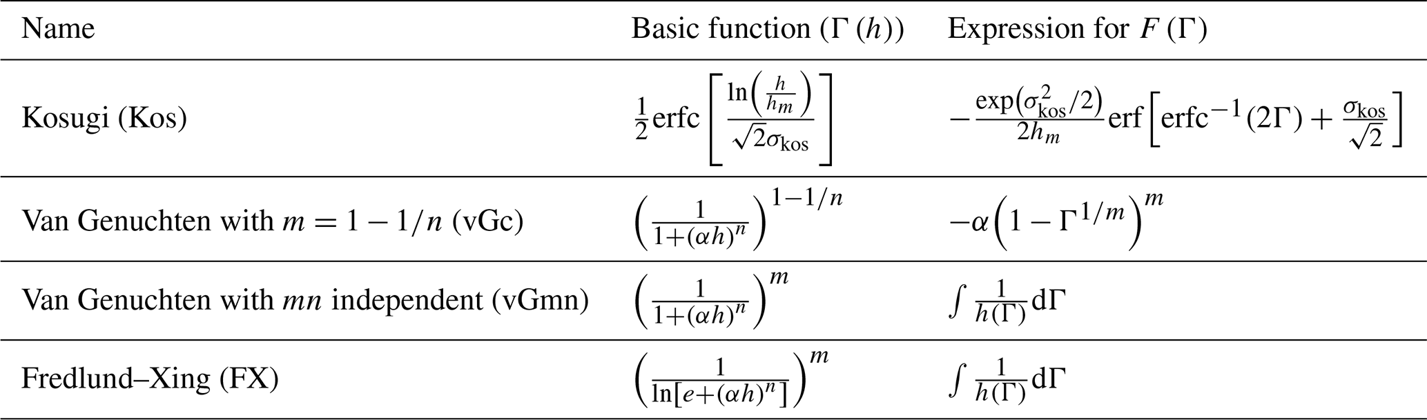
Dependent on the selected WRC parametrization, F in Eq. (19) can be expressed in closed form or must be calculated numerically. For this study, we used four unimodal models to describe the WRC and correspondingly to predict K(h). All four models are used within the PDI system. The basic capillary saturation functions are given by the function of Kosugi (1996), the van Genuchten functions (van Genuchten, 1980) with the usual constraint ($m=\mathrm{1}-\mathrm{1}/n$) and also in unconstrained form (m independent from n), and the Fredlund and Xing (1994) saturation function. The latter is the function given in the last row of Table 2. The models are referred to as Kos-PDI, vGc-PDI, vGmn-PDI, and FX-PDI. The saturation functions and the solutions for the integral F are given in Table 2. For the Kos and vGc saturation functions, F is given in analytical form. For the unconstrained vGmn and FX saturation functions, F needs to be evaluated using numerical integration. We chose these four functions as they are the most commonly used functions in the field of soil hydrology and geotechnics.

Although the derivation of K_c(h) is presented here for the PDI model, we note that the model concept is not limited to PDI-type soil hydraulic functions and that closed-form expressions can also be derived easily for “classical” models that use a residual water content and neglect the non-capillary components. For those cases, the expression for the integral F(Γ₀) is zero. For the original van Genuchten–Mualem model with constraint $m=\mathrm{1}-\frac{\mathrm{1}}{n}$, one obtains, for example,

$$\begin{array}{}\text{(21)}& K\left(h\right)=\mathit{\beta }{\mathit{\tau }}_{\mathrm{s}}{S}_{\mathrm{e}}^{\mathit{\lambda }}({\mathit{\theta }}_{\mathrm{s}}-{\mathit{\theta }}_{\mathrm{r}}{)}^{\mathrm{2}}{\left[\mathit{\alpha }\left\{\mathrm{1}-(\mathrm{1}-S_{\mathrm{e}}^{\frac{\mathrm{1}}{m}}{)}^m\right\}\right]}^{\mathrm{2}},\end{array}$$

where S_e is the effective saturation function ($S_{\mathrm{e}}=\left(\mathit{\theta }-{\mathit{\theta }}_{\mathrm{r}}\right)/\left({\mathit{\theta }}_{\mathrm{s}}-{\mathit{\theta }}_{\mathrm{r}}\right))$, or simply

$$\begin{array}{}\text{(22)}& K_{\mathrm{s}}=\mathit{\beta }{\mathit{\tau }}_{\mathrm{s}}{\left.{\left(\mathit{\theta }\right.}_{\mathrm{s}}-{\mathit{\theta }}_{\mathrm{r}}\right)}^{\mathrm{2}}{\mathit{\alpha }}^{\mathrm{2}}.\end{array}$$

Table 2 Summary of the basic water retention functions used in the PDI scheme (see Appendix A1) as well as the analytical solutions for F (Eq. 19) as given in Peters (2014). The parameters α, n, m, σ_kos, and h_m are shape parameters, and e is the Euler number. In the case of FX and vGmn, no analytical solution for the integral in Eq. (19) is known, and F must be evaluated numerically.

3 Materials and methods

3.1 Soil hydraulic models

The water retention and unsaturated hydraulic conductivity functions were described using the PDI model system with four different unimodal basis functions for capillary water (Table 2), combined with the Mualem (1976a) capillary bundle model to predict the shape of the capillary conductivity function, K_c(h). This function is given by Eq. (19) and included in the total conductivity function given by Eq. (1). The relative tortuosity parameter λ was set to 0.5 following Mualem (1976a), $\mathit{\beta }=\mathrm{3.04}\times {\mathrm{10}}^{-\mathrm{4}}$ m³ s⁻¹ (Sect. 2.2, Table 1), and τ_s is the new unknown tortuosity parameter. K_nc and K_v were predicted from the WRC (Peters et al., 2021; see Appendix A1).

For soils with a wide pore-size distribution, Mualem's model (as all capillary bundle models) in combination with water retention models that gradually approach saturation can produce a non-physical sharp decrease in the hydraulic conductivity near saturation (e.g., Vogel et al., 2000; Ippisch et al., 2006). Madi et al. (2018) developed a mathematical criterion to test individual WRC parameterizations for physical plausibility. To avoid this model artifact, we used the “hclip approach” of Iden at al. (2015) in all cases. The hclip approach limits the pore size in the conductivity prediction integral to a maximum value, which is equivalent to a minimum suction, h_crit. According to Jarvis (2007), we use h_crit= 0.06 m, corresponding to an equivalent diameter of 0.5 mm (see also Sect. 2.4).

3.2 Estimating the saturated tortuosity coefficient, τ_s

To obtain an estimate for τ_s, reliable data for the WRC and in particular for the HCC in the wet range (but not at saturation) are needed. We used six data sets used by Peters (2013) and six additional data sets from Sarkar et al. (2019), which fulfill the abovementioned requirements. Soil textures varied from pure sand to loamy clay, representing a wide variety of different soils. Details about the soils are given in the original literature and are summarized in Table 3. For each of the four PDI combinations with the capillary saturation functions given in Table 2, we determined a value for τ_s by fitting them to the 12 data sets and estimating the WRC parameters and τ_s. The median values of the estimated τ_s values were used in the corresponding prediction models.

3.3 Validation of the absolute K predictions

To test the predictions of K(h) from the WRC, we selected data sets that cover a relatively wide moisture range and could be described well using unimodal WRCs. We used 23 data sets, which were obtained at Technische Universität Braunschweig, Germany. The data comprised again a broad range of textural classes. Some of them stemmed from soil columns taken at the same sites at which the soil columns of Sarkar et al. (2019) were taken (locations JKI, GG, and SAU). However, we used independent data from different soil samples taken in different years. All data sets except one (Test 4) are from undisturbed samples. Details about the validation data are given in Table 4.

Table 3 Calibration data sets used for estimating water retention curves and the saturated tortuosity coefficient τ_s.

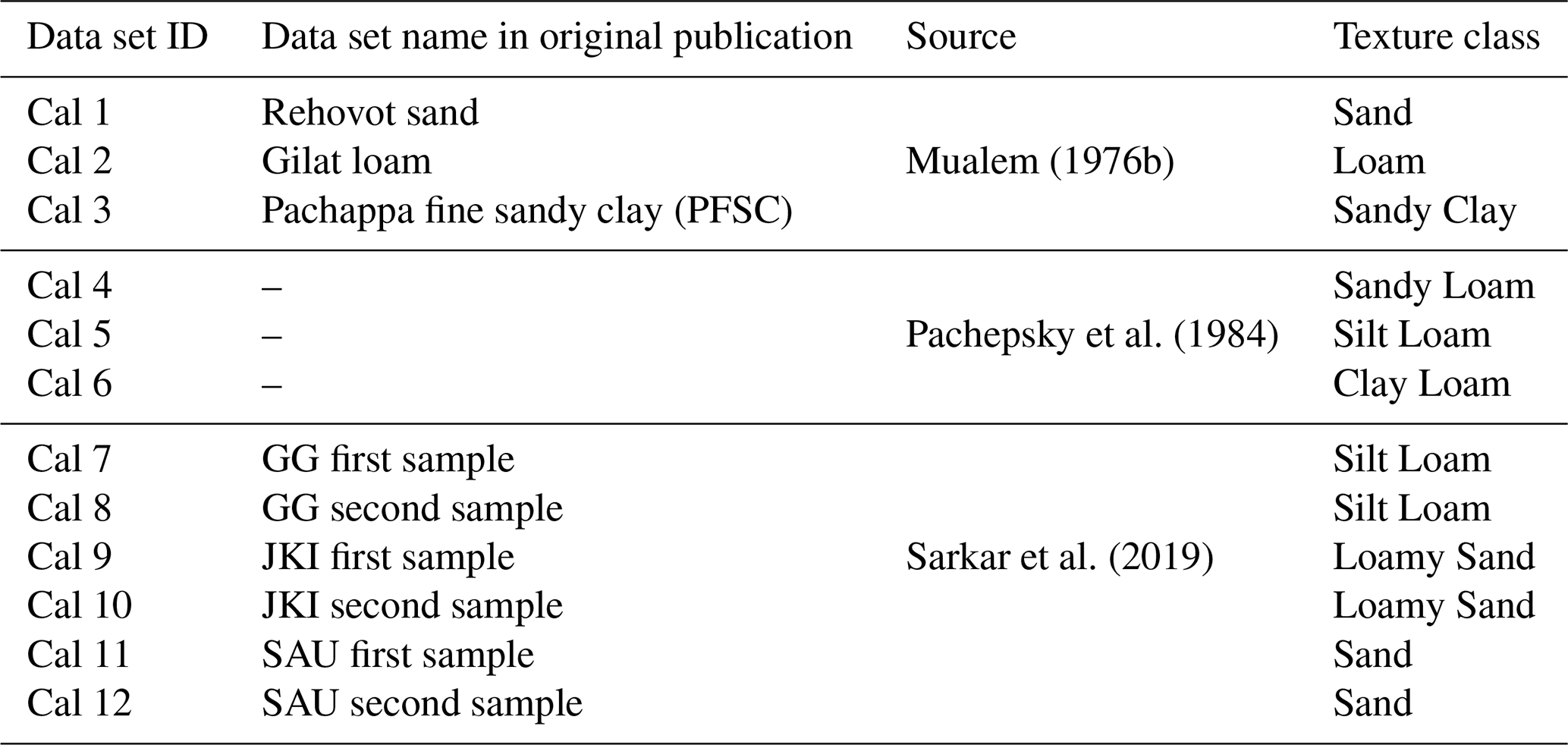
Table 4 Test data sets used to test the conductivity predictions.

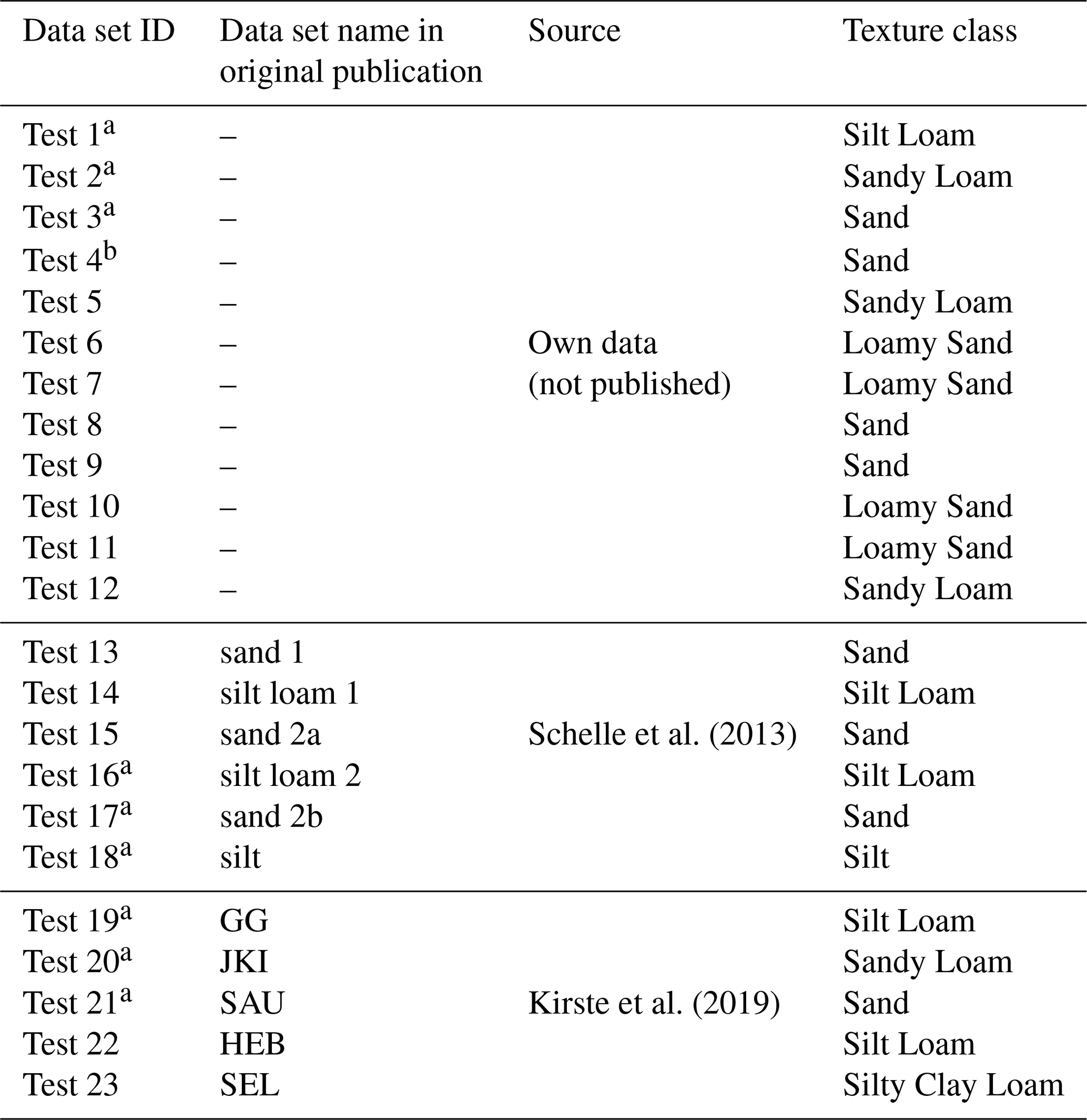
^a samples taken at same sites but different years as some of the calibration data (Cal 7 to Cal 12). ^b disturbed sample.

3.4 Parameter estimation and diagnostics

The models were fitted to the data by minimizing the sum of weighted squared residuals between modeled and measured data (Peters, 2013):

$$\begin{array}{}\text{(23)}& \begin{array}{rl}\mathit{\varphi }\left(\mathit{b}\right)& =w_{\mathit{\theta }}{\sum }_{i=\mathrm{1}}^{n_{\mathit{\theta }}}{\left[{\mathit{\theta }}_i-{\mathit{\theta }}_{\mathrm{mod},i}\left(\mathit{b}\right)\right]}^{\mathrm{2}}\\ & +w_K{\sum }_{i=\mathrm{1}}^{n_K}{\left[{\log }_{\mathrm{10}}\left(K_i\right)-{\log }_{\mathrm{10}}\left({\stackrel{\mathrm{̃}}{K}}_i\right(\mathit{b}\left)\right)\right]}^{\mathrm{2}},\end{array}\end{array}$$

where θ_i and θ_mod,i are the measured and modeled water contents, K_i and ${\stackrel{\mathrm{̃}}{K}}_i$ are measured and modeled hydraulic conductivities, n_θ and n_K are the respective number of data points, w_θ=10 000 and w_K=16 are weights for the two data groups (Peters, 2011), and b is the vector of unknown model parameters. The shuffled-complex-evolution algorithm SCE-UA (Duan et al., 1992) was used to minimize the objective function given by Eq. (23). In the case of estimating the general value of τ_s, the parameter vector contained all adjustable parameters of the water retention function plus τ_s. In the case of the hydraulic conductivity predictions, w_K was set to 0, and the estimated parameter vector contained only the WRC parameters. The performance of the different approaches was compared in terms of the root-mean-square error (RMSE) for the WRC and the HCC (common log of K(h)), respectively. Model comparisons were based on the Akaike information criterion, AICc, corrected for small sample sizes (Hurvich and Tsai, 1989).

4 Results and discussion

4.1 Empirical estimate of the saturated tortuosity coefficient τ_s

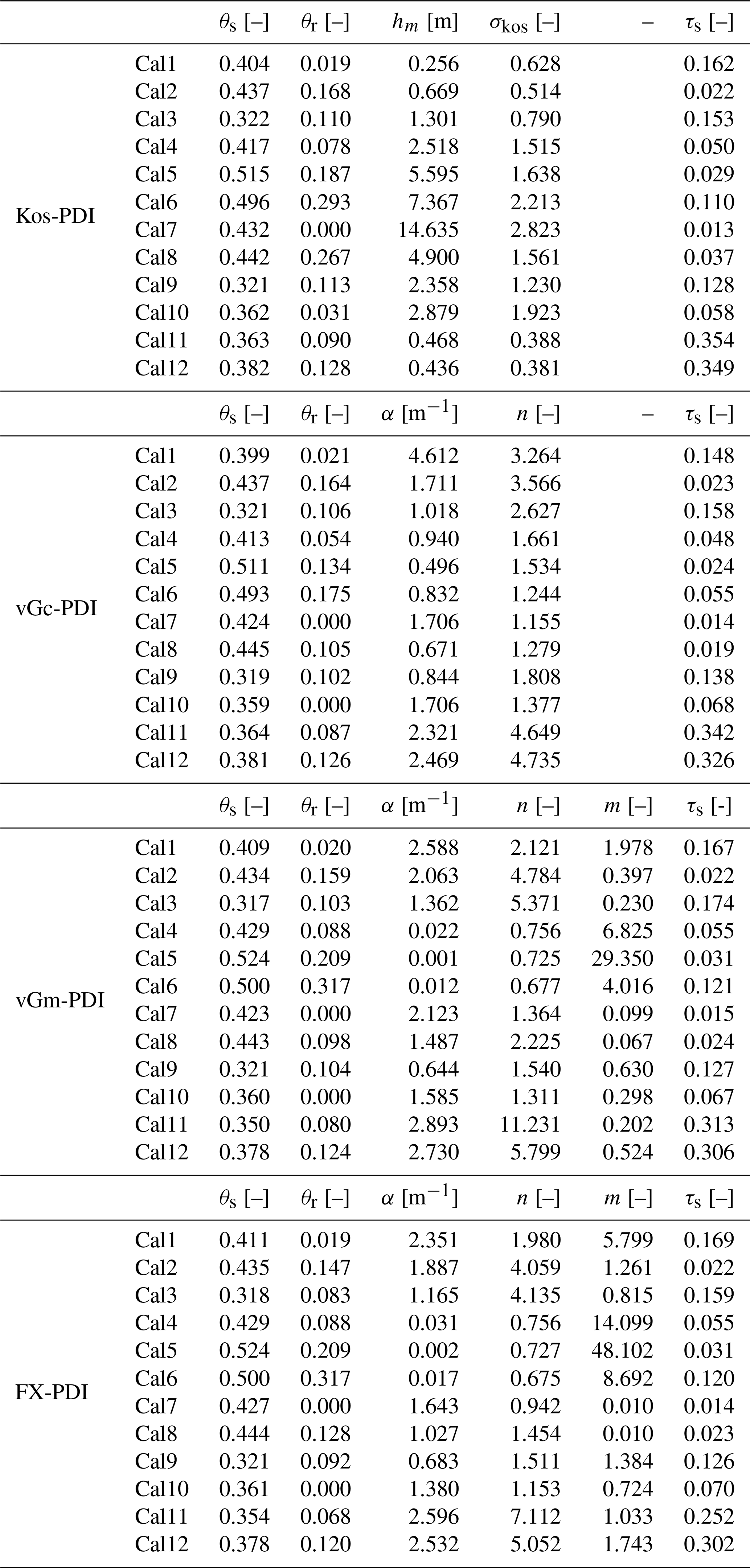
Figure 2 illustrates, using 4 of the 12 calibration data sets described in Table 3, the fitted water retention and conductivity functions for the four basic hydraulic models listed in Table 2. A full overview on all calibration data sets and the fitted models is given in the Supplement. All estimated parameters are given in Table A1. In general, all four models are well suited to describe the data. Actually, the models can be hardly distinguished on the plots since they lie largely on top of each other. Figure 3 shows the corresponding distributions of RMSE_θ and RMSE_logK, which allow one to better differentiate the fitting performance. Results confirm the visual impression from Fig. 2 that all four models fit similarly, with a slightly better performance of the models having six free parameters (i.e., FX-PDI and vGmn-PDI) as compared to those with five free parameters (vGc-PDI and Kos-PDI). We note that fitting the K functions of Peters et al. (2021), using K_s instead of τ_s as an adjustable parameter and leaving all other settings identical, would lead here exactly to the same results.

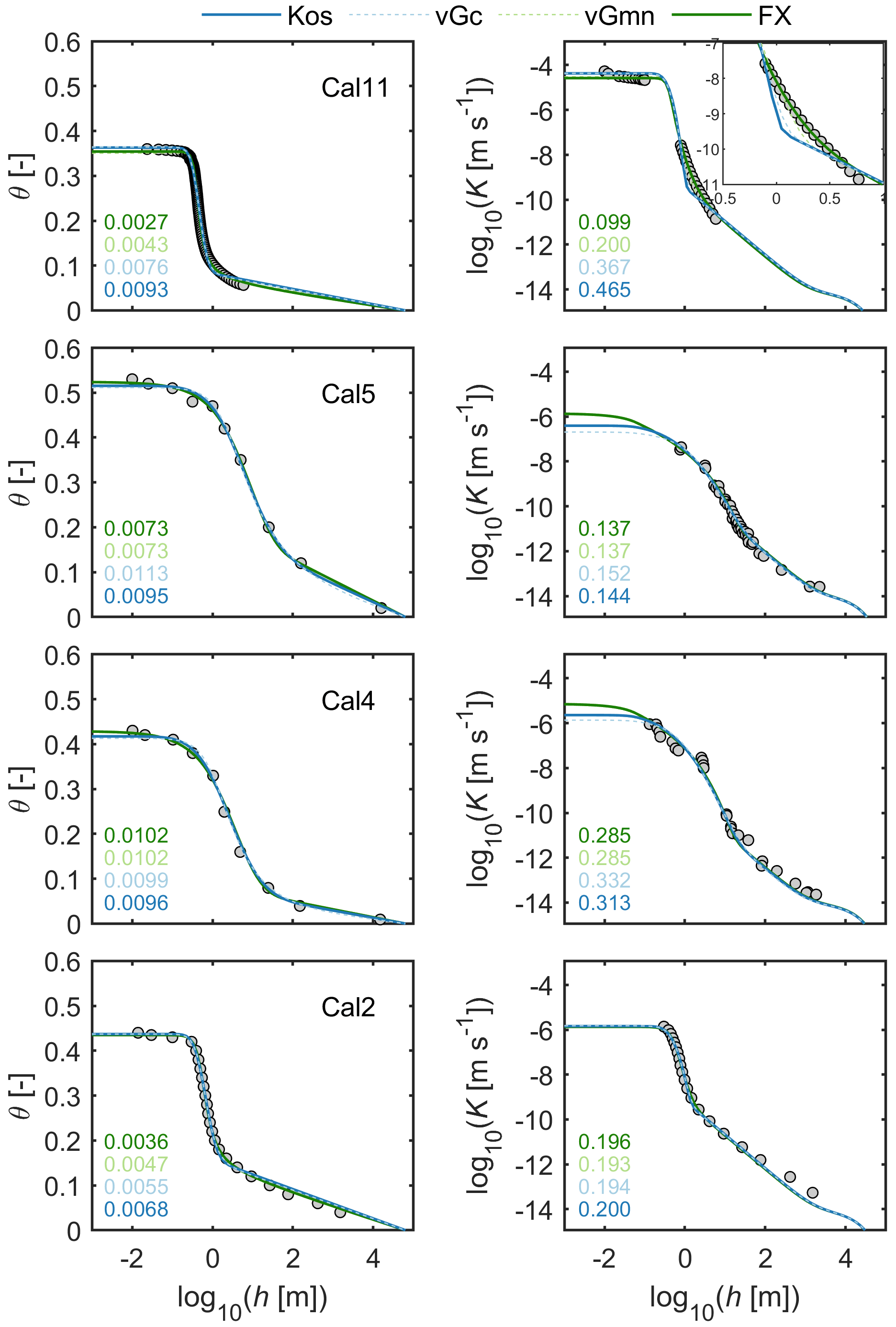
Figure 2 Plots of 4 of the 12 calibration data sets and the fitted water retention and conductivity functions used to calibrate the saturated tortuosity coefficient τ_s in Eq. (19). Parameter λ was set to a value of 0.5 according to Mualem (1976a). Parameter τ_s and the retention parameters were allowed to vary. Numbers in the subplots indicate RMSE_θ and RMSE_logK values for the various model combinations.

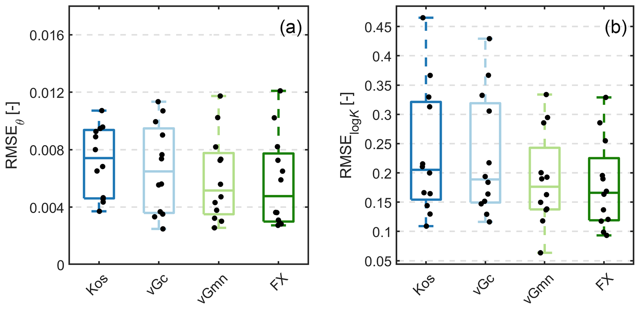
Figure 3 Distributions of RMSE_θ and RMSE_logK of the fitted retention and conductivity models for the 12 data sets. Black dots indicate single realizations.

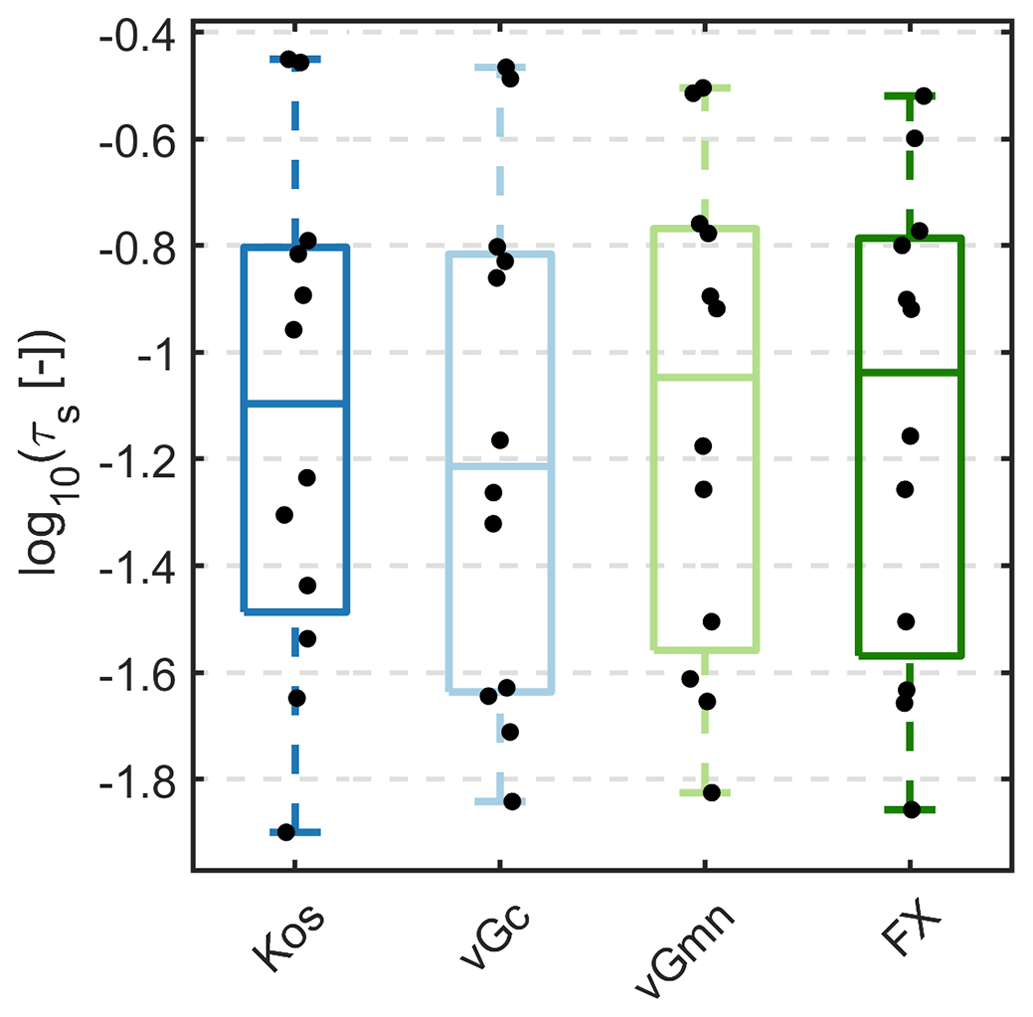
The distributions of the resulting values for τ_s for the four models are shown in Fig. 4. The median values for τ_s were 0.062 for the constrained van Genuchten function (vGc), 0.084 for the Kosugi function (Kos), and 0.094 and 0.095 for the unconstrained van Genuchten (vGmn) and Fredlund–Xing (FX) functions, respectively. It appears noteworthy that the two best-fitting WRC models yield almost identical estimates of τ_s. The range of τ_s for the 12 data sets spanned less than 1.5 orders of magnitude. We interpret this as an indication that the hypothesis of relatively moderate overall variability in τ_s may be justified. When fitting the classic PDI scheme (with K_s as a fitting parameter) to these data, which do not include measured conductivity data at saturation, the estimated K_s values varied by more than 3 orders of magnitude. In natural soils, the measured K_s values can vary even more due to the dominance of (texture-independent) structural pores and macropores on K_s (e.g., Usowicz and Lipiec, 2021).

Figure 4 Distribution of fitted values of τ_s for 4 different retention functions.

4.2 Tests of the absolute conductivity predictions

By using median values of τ_s for the different models (0.084, 0.062, 0.094, and 0.095 for Kos-PDI, vGc-PDI, vGmn-PDI, and FX-PDI, respectively; Fig. 4), we predicted the hydraulic conductivity functions from the water retention functions for 23 test data sets. In Fig. 5, we show the resulting distributions of RMSE_θ (fitted) and RMSE_logK (predicted). Since measured conductivities were available primarily within the range where the capillary conductivity component dominates, RMSE_logK can be interpreted as an approximate error of the capillary conductivity prediction. The medians of RMSE_logK for the Kos-PDI and vGc-PDI models were 0.71 and 0.67, respectively. Combinations with the more flexible retention models yielded median RMSE_logK values of 0.49 for vGmn-PDI and 0.40 for FX-PDI. To test whether conductivity predictions were biased, we calculated also the mean error (Fig. 6). For the FX-PDI model, the median was close to zero, indicating an unbiased conductivity prediction, whereas the other models tended to underestimate the conductivity data.

Figure 7 shows fitted WRCs and predicted HCCs along with the measured conductivity data. Due to space limitations, only a subset of six randomly selected cases is shown for the FX-PDI combination. The WRC fits and HCC predictions for all 23 test soils and all four models are listed in the Supplement.

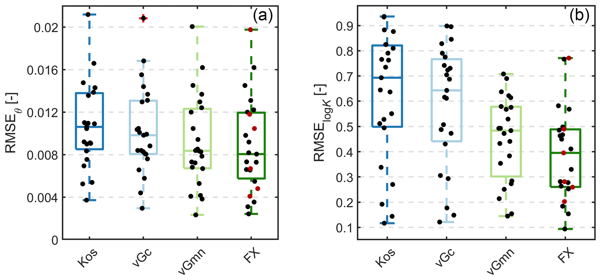
Figure 5 RMSE_θ and RMSE_logK for prediction of the absolute conductivity from the soil water retention function of 23 test data sets. Black dots indicate the validation data sets; red dots indicate the data sets used to estimate a general value of the saturated tortuosity coefficient τ_s. The red cross indicates an outlier, defined by the MATLAB^® default settings as 1.5 times the interquartile range away from the top or bottom of the box (https://de.mathworks.com/help/matlab/ref/boxchart.html, last access: 13 April 2023).

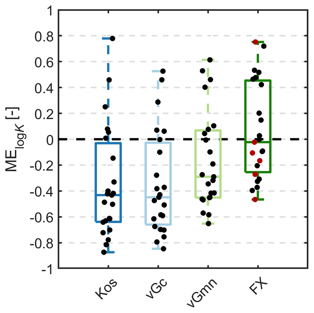
Figure 6 Mean errors of the predicted absolute conductivity based on the soil water retention function for 23 test data sets. Black dots indicate all 23 validation data sets; red dots indicate data sets shown in Fig. 7.

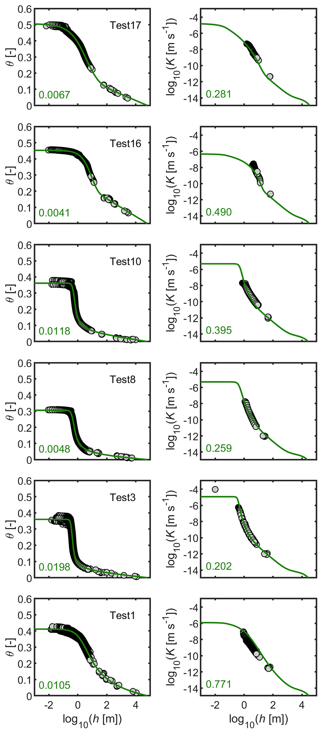
Figure 7 Measured data (dots), fitted retention functions (a, c) and predicted conductivity functions (b, d). Shown are for six randomly selected soils out of 23 validation data sets. Numbers in the subplots indicate RMSE_θ and RMSE_logK values Note that the conductivity curves are not fits to the data.

4.3 Improved estimation of K functions when K data are available

Several authors (e.g., Schaap and Leij, 2000; Peters et al., 2011) have stressed that the tortuosity parameter λ might differ greatly from the value suggested by Mualem (1976a), since the change in tortuosity with respect to capillary saturation can obviously be different for different soils. The new scheme is valuable not only for cases where no or insufficient information about the conductivity is available. It is also useful when data are available for the unsaturated hydraulic conductivity but are missing in the wet range. This is the case, for example, with the commonly used evaporation method (Schindler, 1980; Peters and Durner, 2008b; Peters et al., 2015). Then, there is often high uncertainty in the wet moisture range; thus, an unrealistic conductivity extrapolation might result (see Fig. 1, bottom). In such cases, λ might be estimated, and only τ_s might be fixed. We illustrate this in Fig. 8 for the data set shown in Fig. 1 (bottom). Again, the vGmn-PDI retention model is used, but instead of Eq. (16), we now use Eq. (18) with τ_s=0.094. Now, the model is well able to be fitted to the data, and the hydraulic conductivity close to saturation is more reasonably predicted as in Fig. 1: predicted conductivity at saturation is $\mathrm{1.7}\times {\mathrm{10}}^{-\mathrm{7}}$ m s⁻¹ (or 1.5 cm d⁻¹) for the original and $\mathrm{1.3}\times {\mathrm{10}}^{-\mathrm{5}}$ m s⁻¹ (or 112 cm d⁻¹) for the new scheme. Note that the new scheme has one less adjustable parameter.

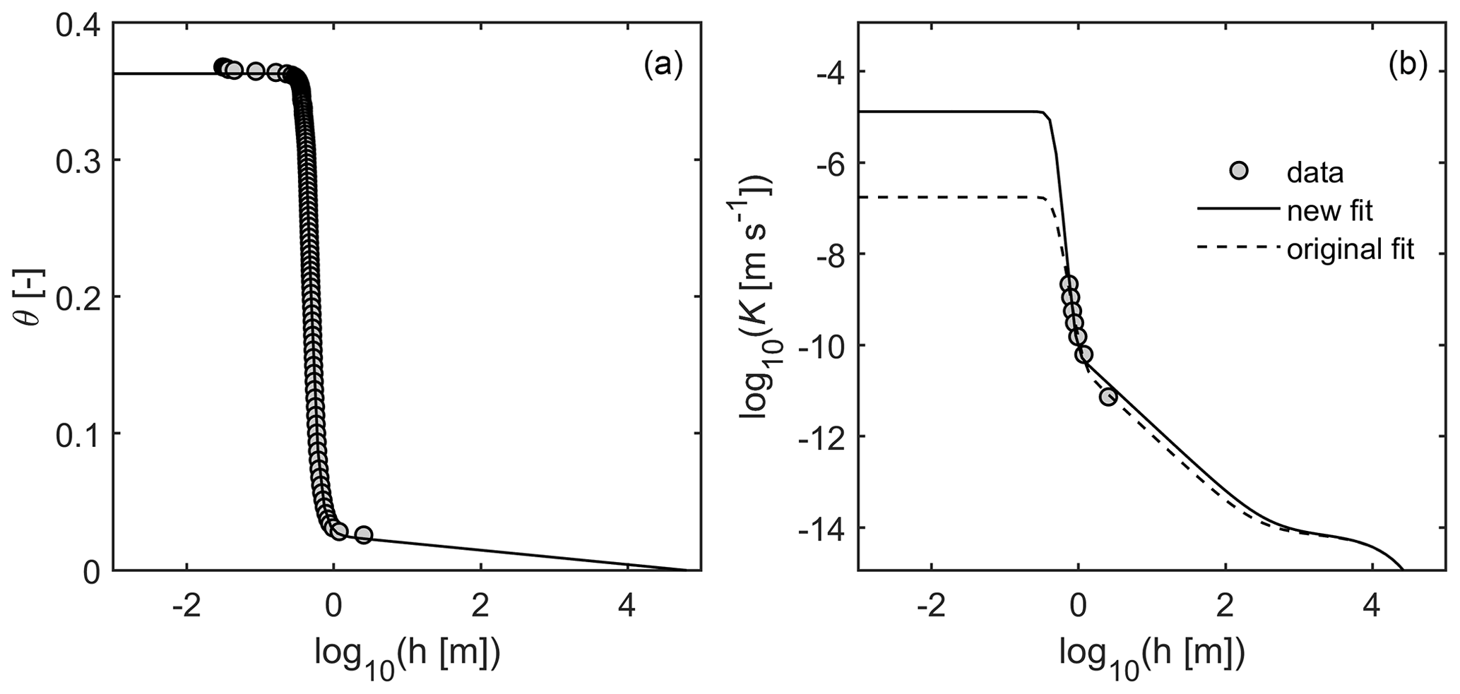
Figure 8 Same data as in Fig. 1c and d. A new scheme with vGmn as basic retention function and τ_s fixed at 0.094 was fitted to the data (new fit). For comparison, the original fit using K_s as adjustable parameter is given by dashed lines. Note that the new scheme has one adjustable parameter less.

4.4 Considerations of the hydraulic conductivity at saturation

Because the saturated hydraulic conductivity is relatively easy to measure, many determine K_s experimentally. As emphasized earlier, the use of K_s for scaling the relative hydraulic conductivity function should be avoided as much as possible. Still, K_s provides valuable information for the hydraulic behavior of soils at and close to saturation, which cannot be derived from the WRC. Within the context of modeling macropore flow, Nimmo (2021) identified a need for approaches to determine the properties of the matrix only while excluding the remainder of the porous medium. Predictions of a capillary conductivity function may help to fill this research gap.

Our approach predicts the capillary hydraulic conductivity in the matrix domain up to a minimum suction. Following Jarvis (2007), we may choose for this a suction of about 0.06 m (pore diameter approximately 0.5 mm) up to which the macropore conductivity can be neglected. Accordingly, we call the conductivity at h_crit = 0.06 m the “saturated matrix conductivity” (K_s,matrix). Knowledge of K_s,matrix could substantially improve the parameterization of simulation models that explicitly distinguish between matrix and macropore flow (e.g., Reck et al., 2018; van Schaik et al., 2010).

The shape of the conductivity function in the macropore-affected range cannot be predicted using capillary bundle models (Durner, 1994). Thus, it is preferable to cover the region between K_s,matrix and the measured K_s using some interpolation function such as proposed by Schaap and van Genuchten (2006). Using the abovementioned value of 0.06 m for h_crit as a starting point for the interpolation and assuming that the saturated conductivity (K_s) is reached at a pore diameter of 5 mm (i.e., at h_s= 0.006 m), we can formalize the interpolation as

$$\begin{array}{}\text{(24)}& K=\left\{\begin{array}{lll}{K}_{\mathrm{s},\mathrm{matrix}}& \mathrm{for}& h=h_{\mathrm{crit}},\\ K_{\mathrm{int}}& \mathrm{for}& h_{\mathrm{crit}}>h>h_{\mathrm{s}},\\ K_{\mathrm{s}}& \mathrm{for}& h\le h_{\mathrm{s}}.\end{array}\right.\end{array}$$

As an example, we illustrate the interpolation with a simple smooth cosine interpolation function, with the log of the suction in the argument (Fig. 9). Mathematically, this interpolation is expressed as

$$\begin{array}{}\text{(25)}& y_{\mathrm{int}}=y_{\mathrm{crit}}+\mathrm{0.5}\left[\cos \left(\mathit{\pi }{\displaystyle \frac{\left(x-x_{\mathrm{s}}\right)}{\left(x_{\mathrm{crit}}-x_{\mathrm{s}}\right)}}\right)+\mathrm{1}\right]\left(y_{\mathrm{crit}}-y_{\mathrm{s}}\right),\end{array}$$

with the transformed variables y=log (K) and x=log(h) and consideration of the corresponding subscripts. We note that the real course of the K(h) function in this moisture region probably will be different; hence, other interpolation schemes could be used. Still, any interpolation will probably improve the performance of numerical models if such conditions close to full saturation are encountered.

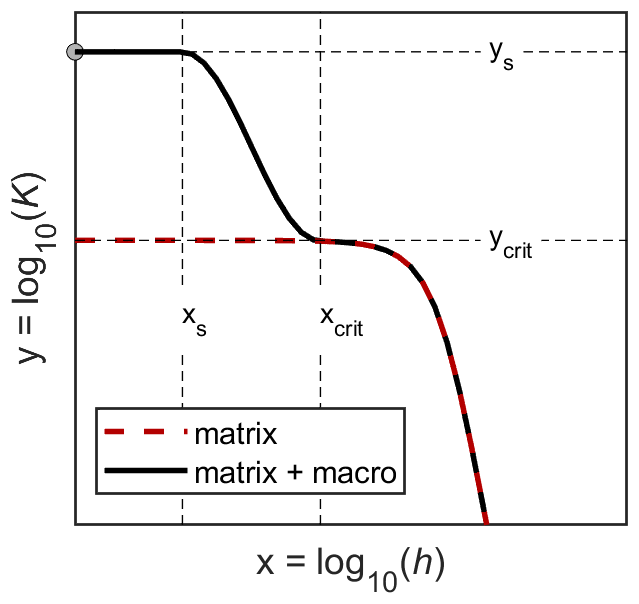
Figure 9 Interpolation scheme between the predicted capillary conductivity (red dashed line) and the measured value of K_s (gray dot).

Figure 10 shows the practical application of the above interpolation scheme for the data given in Fig. 1 (top). The PDI water retention function was fitted to the retention data, while K(h) was predicted from the WRC from dryness to h= 0.06 m. From h=0.06 m to h=0.006 m, the smooth interpolation scheme (Eq. 24) was applied. With this scheme, we obtained a description of hydraulic conductivity from oven dryness to full saturation.

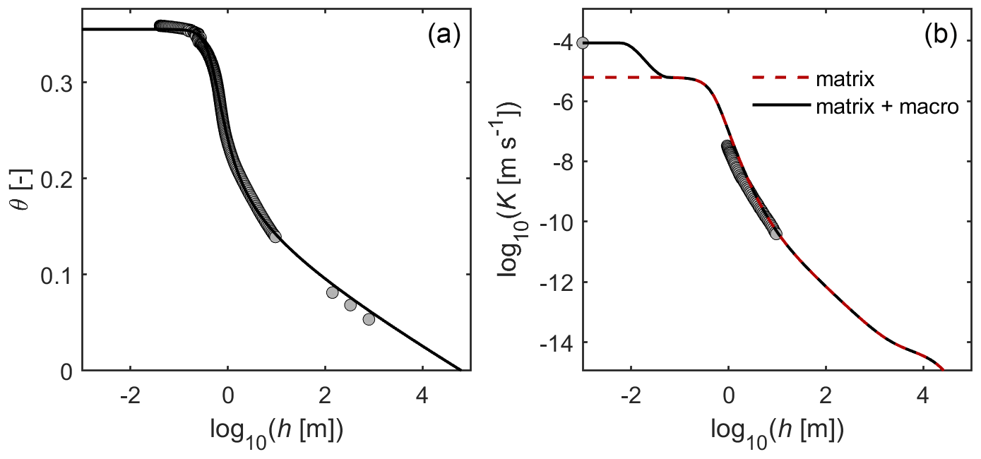
Figure 10 Application of the interpolation scheme given by Eq. (24) to the data set shown in Fig. 1a and b. The FX-PDI model was fitted to the water retention data and K(h) was predicted from dryness to h=0.06 m.

5 Summary and conclusions

The unsaturated hydraulic conductivity of soils is still the most difficult hydraulic property to directly measure. The availability of commercial systems that allow one to determine SHPs using the simplified evaporation method has improved the situation somewhat; still, available conductivity data generally are restricted to a relatively limited soil moisture range so that predictive models for the hydraulic conductivity curve continue to play a critical role. To date, such predictions mostly use pore-bundle models that require measured conductivity data to scale the predicted curves. However, the HCC outside the range for which measured data are available is highly uncertain. In this contribution we presented a prediction scheme for the hydraulic conductivity covering the moisture range from very dry conditions to almost full saturation. The PDI modeling framework predicts three components of the conductivity, namely, vapor, non-capillary, and capillary liquid conductivity as absolute values from the water retention function.

Pore-bundle models do not in themselves account for important characteristics such as path elongation due to tortuosity, surface roughness of pore walls, non-circular capillaries, dead-end pores, physical properties of the liquid phase, etc. These effects can be accounted for with a parameter that is called tortuosity coefficient. We divide this parameter into two factors: a saturated tortuosity factor and a relative tortuosity function that takes the dependence of tortuosity on water content into account. The saturated tortuosity factor is shown to vary little among different soils, and we have determined a universal value empirically from data. The new scheme using a saturated tortuosity factor with an assigned universal value can be used to predict the hydraulic conductivity curve from the water retention curve when insufficient or no conductivity data are available.

The proposed general prediction scheme was tested by combining it with four parametric water retention models. Of these, the PDI model with the Fredlund and Xing (1994) basic saturation function and the model of van Genuchten with independent parameters m and n as basic function performed best. The identified value for the saturated tortuosity coefficient τ_s was 0.095. From a practical point of view, τ_s may simply be set to 0.1. The prediction accuracy with the new model was tested using a set of 23 soils for which measured K values were available. For the best-performing model FX-PDI, the predictions matched the measured data on average with a RMSE_logK of about 0.4, without a bias between the predicted functions and measured data.

The conductivity estimation using our approach involves the conductivity of the soil matrix only and as such excludes the effects of the soil structure. The scheme is applicable only if retention data are available, and it opens new possibilities to use existing retention data collections (e.g., Gupta et al., 2022). The approach will also be helpful for situations where a measured value of the saturated conductivity K_s is available and where soil structure plays a role (which is the rule for most topsoils). In such cases, the predicted HCC can be combined with an interpolation towards K_s to obtain a well-estimated conductivity function over the full moisture range. Differentiating between structural and textural effects enables a physically more consistent use of measured SHP information.

In the cases where measured unsaturated conductivity data are available (such as from the simplified evaporation method), the proposed model with fixed τ_s can be fitted by adjusting a soil-specific relative tortuosity coefficient. This leads to a more reliable description of the conductivity function in the wet range, where no data are available, relative to current model approaches. Our new scheme can therefore improve the fitting of SHP models to measurements and can be implemented easily in the standard optimization software packages.

Appendix A

A1 The PDI model system

A1.1 PDI water retention function

The capillary saturation function S_c [–] and a non-capillary saturation function S_nc [–] may be superimposed in the following form (Iden and Durner, 2014):

$$\begin{array}{}\text{(A1)}& \mathit{\theta }\left(h\right)=({\mathit{\theta }}_{\mathrm{s}}-{\mathit{\theta }}_{\mathrm{r}})S_{\mathrm{c}}+{\mathit{\theta }}_{\mathrm{r}}{S}_{\mathrm{nc}},\end{array}$$

in which the first right-hand term holds for water stored in capillaries, and the second term holds for water stored in adsorbed water films and pore corners. θ [m³ m⁻³] is the total water content, h [m] is the suction head, and θ_s [m³ m⁻³] and θ_r [m³ m⁻³] are the saturated and maximum adsorbed water contents, respectively. To meet the physical requirement that the capillary saturation function reaches zero at oven dryness, a basic saturation function Γ(h) is scaled by (Iden and Durner, 2014)

$$\begin{array}{}\text{(A2)}& S_{\mathrm{c}}\left(h\right)={\displaystyle \frac{\mathrm{\Gamma }\left(h\right)-\mathrm{\Gamma }\left(h_{\mathrm{0}}\right)}{\mathrm{1}-\mathrm{\Gamma }\left(h_{\mathrm{0}}\right)}},\end{array}$$

with h₀ [m] being the suction head at oven dryness, which can be set to 10^4.8 m following Schneider and Goss (2012). Γ(h) can be any unimodal or multimodal saturation function such as the unimodal functions of van Genuchten (1980) and Kosugi (1996) or their bimodal versions (Durner, 1994; Romano et al., 2011).

The saturation function for non-capillary water is given by a smoothed piecewise linear function (Iden and Durner, 2014), which is here given in the notation of Peters et al. (2021):

$$\begin{array}{}\text{(A3)}& S_{\mathrm{nc}}\left(h\right)={\displaystyle \frac{\ln \left(\frac{h_{\mathrm{0}}}{h}\right)-b\ln \left(\mathrm{1}+{\left[\frac{h_a}{h}\right]}^{\mathrm{1}/b}\right)}{\ln \left(\frac{h_{\mathrm{0}}}{h_a}\right)}},\end{array}$$

in which the parameter h_a [m] reflects the suction head where non-capillary water reaches its saturation (fixed in our study to the suction at which capillary saturation reaches 0.75). We note that in earlier publications, we set $h_a={\mathit{\alpha }}^{-\mathrm{1}}$ for the constrained van Genuchten function. For the vGmn and the FX models, however, α⁻¹ may be very high although the capillary saturation decreases already at low suctions. Setting $h_a={\mathit{\alpha }}^{-\mathrm{1}}$ would lead in such cases to unrealistic retention functions with S_nc being close to unity, whereas S_c is already close to zero. The calculation scheme for h_a as a quantile of S_c is given in Appendix A2. The parameter h₀ in Eq. (A3) is the suction head where the water content reaches zero, which reflects the suction at oven-dry conditions. S_nc(h) increases linearly from zero at oven dryness to its maximum value of 1.0 at h_a, and it then remains constant towards saturation. In order to ensure a continuously differentiable water capacity function, S_nc(h) must be smoothed around h_a, which is achieved by the smoothing parameter b [–] (Iden and Durner, 2014), given here by

$$\begin{array}{}\text{(A4)}& b=b_o\left(\mathrm{1}+\mathrm{2}{\displaystyle \frac{\mathrm{1}-e^{-b_{\mathrm{1}}}}{n^{\mathrm{2}}}}\right),\end{array}$$

where b_o=0.1 ln (10), and $b_{\mathrm{1}}={\left(\frac{{\mathit{\theta }}_{\mathrm{r}}}{{\mathit{\theta }}_{\mathrm{s}}-{\mathit{\theta }}_{\mathrm{r}}}\right)}^{\mathrm{2}}$.

A1.2 PDI hydraulic conductivity

The PDI hydraulic conductivity model is expressed as (Peters et al., 2021)

$$\begin{array}{}\text{(A5)}& K\left(h\right)=K_{\mathrm{s},\mathrm{c}}{K}_{\mathrm{r},\mathrm{c}}+K_{\mathrm{nc}}+K_{\mathrm{v}},\end{array}$$

where K_r,c [–] is the relative conductivity for the capillary component, K_s,c [m s⁻¹] is the saturated conductivity for the capillary components, and K_nc and K_v [m s⁻¹] are the non-capillary and isothermal vapor conductivities, respectively. K_nc is given by (Peters et al., 2021)

$$\begin{array}{}\text{(A6)}& K_{\mathrm{nc}}=c{\mathit{\theta }}_m{h}_a^{-\mathrm{1.5}}{\left({\displaystyle \frac{h_{\mathrm{0}}}{h_a}}\right)}^{-\mathrm{1.5}(\mathrm{1}-S_{\mathrm{nc}})},\end{array}$$

in which c is used to account for several physical and geometrical constants and being either a free fitting parameter to scale K_nc or $c=\mathrm{1.35}\times {\mathrm{10}}^{-\mathrm{8}}$ m${}^{\mathrm{5}/\mathrm{2}}$ s⁻¹. Parameter θ_m [–] is the water content at h=10³ m. We refer to Saito et al. (2006) or Peters (2013) for details regarding the formulation of K_v as a function of the invoked WRC. Note that the capillary liquid conductivity is formulated as a relative conductivity, which has to be scaled with a measured value, whereas the non-capillary conductivity and the isothermal vapor conductivity are formulated as absolute conductivities.

The relative conductivity for water flow in capillaries is in this paper described using the pore bundle model of Mualem (1976a), which reads in the PDI notation (Peters, 2014) as

$$\begin{array}{}\text{(A7)}& K_{\mathrm{r},\mathrm{c}}\left(S_{\mathrm{c}}\right)={\left(S_{\mathrm{c}}\right)}^{\mathit{\lambda }}{\left[{\displaystyle \frac{{\int }_{{\mathrm{\Gamma }}_{\mathrm{0}}}^{\mathrm{\Gamma }}{h}^{-\mathrm{1}}\mathrm{d}X}{{\int }_{{\mathrm{\Gamma }}_{\mathrm{0}}}^{\mathrm{1}}{h}^{-\mathrm{1}}\mathrm{d}X}}\right]}^{\mathrm{2}},\end{array}$$

where λ [–] is the tortuosity and connectivity parameter, and X is a dummy variable of integration.

A2 Calculation of h_a as a function of the S_c quantile

Peters (2013) proposed two methods to define the critical tension h_a (m) for the non-capillary saturation function S_nc (–). He decided to set $h_a={\mathit{\alpha }}^{-\mathrm{1}}$ for van Genuchten's model and h_a=h_m for Kosugi's model (1996). His second option was to define h_a as a quantile of the capillary saturation function, while suggesting the value of 0.5 as a potential choice. For completeness, we repeat here the relevant equations.

The capillary saturation function of van Genuchten is given by

$$\begin{array}{}\text{(A8)}& \mathrm{\Gamma }\left(h\right)={\left[\mathrm{1}+{\left(\mathit{\alpha }h\right)}^n\right]}^{-m}.\end{array}$$

Recall that this function ensures a saturation of zero at the suction corresponding to oven dryness, h₀ (L). Iden and Durner (2014) proposed to scale Eq. (A8) using the function

$$\begin{array}{}\text{(A9)}& S_{\mathrm{c}}\left(h\right)={\displaystyle \frac{\mathrm{\Gamma }\left(h\right)-{\mathrm{\Gamma }}_{\mathrm{0}}}{\mathrm{1}-{\mathrm{\Gamma }}_{\mathrm{0}}}},\end{array}$$

where ${\mathrm{\Gamma }}_{\mathrm{0}}=\mathrm{\Gamma }\left(h_{\mathrm{0}}\right).$ According to Peters (2013), we define the suction h_a as

$$\begin{array}{}\text{(A10)}& S_{\mathrm{c}}\left(h_a\right)=\mathit{\beta },\end{array}$$

where β [–] represents the chosen quantile of S_c. Combining Eqs. (A8)–(A10) and solving for h_a yields

$$\begin{array}{}\text{(A11)}& h_a={\mathit{\alpha }}^{-\mathrm{1}}{\left[{\mathit{\gamma }}^{-\frac{\mathrm{1}}{m}}-\mathrm{1}\right]}^{\mathrm{1}/n},\end{array}$$

in which the constant γ is defined as

$$\begin{array}{}\text{(A12)}& \mathit{\gamma }=\mathit{\beta }\left(\mathrm{1}-{\mathrm{\Gamma }}_{\mathrm{0}}\right)+{\mathrm{\Gamma }}_{\mathrm{0}}.\end{array}$$

Applying the same approach to the capillary saturation function of Kosugi (1996), i.e.,

$$\begin{array}{}\text{(A13)}& \mathrm{\Gamma }\left(h\right)=\mathrm{0.5}\mathrm{erfc}\left[{\displaystyle \frac{\log \left(\frac{h}{h_{\mathrm{m}}}\right)}{\sqrt{\mathrm{2}}\mathit{\sigma }}}\right],\end{array}$$

yields

$$\begin{array}{}\text{(A14)}& h_a=h_m{e}^{\sqrt{\mathrm{2}}\mathit{\sigma }{\mathrm{erfc}}^{-\mathrm{1}}\left(\mathrm{2}\mathit{\gamma }\right)}.\end{array}$$

Thirdly, for the capillary saturation of Fredlund and Xing (1994), given as

$$\begin{array}{}\text{(A15)}& \mathrm{\Gamma }\left(h\right)={\left[\ln \left(\mathrm{e}+{\left(\mathit{\alpha }h\right)}^n\right)\right]}^{-m},\end{array}$$

we obtain

$$\begin{array}{}\text{(A16)}& h_a={\mathit{\alpha }}^{-\mathrm{1}}{\left(\exp \left({\mathit{\gamma }}^{-\frac{\mathrm{1}}{m}}\right)-e\right)}^{\frac{\mathrm{1}}{n}}.\end{array}$$

Appendix B: Additional information

Table B1 Estimated parameter values for all four model combinations for the calibration data set.