the Creative Commons Attribution 4.0 License.
the Creative Commons Attribution 4.0 License.
 | 03 Apr 2023
Estimating vadose zone water fluxes from soil water monitoring data: a comprehensive field study in Austria
Marleen Schübl
Giuseppe Brunetti
Gabriele Fuchs
Christine Stumpp
Groundwater recharge is a key component of the hydrological cycle, yet its direct measurement is complex and often difficult to achieve. An alternative is its inverse estimation through a combination of numerical models and transient observations from distributed soil water monitoring stations. However, an often neglected aspect of this approach is the effect of model predictive uncertainty on simulated water fluxes. In this study, we made use of long-term soil water content measurements at 14 locations from the Austrian soil water monitoring program to quantify and compare local potential groundwater recharge rates and their temporal variability. Observations were coupled with a Bayesian probabilistic framework to calibrate the HYDRUS-1D model and assess the effect of model predictive uncertainty on long-term simulated recharge fluxes. Estimated annual potential recharge rates ranged from 44 to 1319 mm a−1 with a relative uncertainty (95 % interquantile range/median) in the estimation of between 1 % and 39 %. Recharge rates decreased longitudinally, with high rates and lower seasonality at western sites and low rates with high seasonality and extended periods without recharge at the southeastern and eastern Austrian sites. Higher recharge rates and lower actual evapotranspiration were related to sandy soils; however, climatic factors had a stronger influence on estimated potential groundwater recharge than soil properties, underscoring the vulnerability of groundwater recharge to the effects of climate change.
- Article
(6666 KB) - Full-text XML
- BibTeX
- EndNote


Groundwater is the largest reservoir of liquid freshwater on Earth and one of the most important sources of drinking and irrigation water. Under changing climatic conditions, with extremes occurring more frequently and intensely, the strategic importance of groundwater for global water and food security is expected to further increase (Taylor et al., 2013). In some countries, such as Austria, groundwater (including spring water) is the most important water resource, making up 100 % of the water supply (Vogel, 2001). The major limitation for sustainable groundwater use is recharge, which represents the maximum amount of water that may be withdrawn from an aquifer without depleting it. This makes it a crucial variable for groundwater resource management (Moeck et al., 2020; Taylor et al., 2013). A large portion of groundwater recharge comes from water infiltrating soil and flowing through the vadose zone towards the water table (Döll and Fiedler, 2008; Nolan et al., 2007). Infiltration capacity, root water uptake, and evaporation from the upper soil layers determine the net amount of water which is transported into the deeper vadose zone, following the gradient in matric potential and gravity (Vereecken et al., 2008). Water flow through the vadose zone is supposed to have a major influence on the process of groundwater recharge, even at karst mountain sites (Berthelin et al., 2020; Hartmann et al., 2014; Kaminsky et al., 2021; Neukum et al., 2008).
The quantification of recharge is complicated by temporal and spatial variability and by the fact that direct measurements are difficult (Moeck et al., 2020, 2018; Nolan et al., 2007; Scanlon et al., 2002). Lysimeters are the only means of obtaining local measurements of seepage flow, which can be considered a good indicator of groundwater recharge (Moeck et al., 2020, 2018; Seneviratne et al., 2012; von Freyberg et al., 2015). However, their appropriate setup is difficult without introducing a bias in the hydrological processes (Barkle et al., 2011; Groh et al., 2016; Pütz et al., 2018; Stumpp et al., 2012). Furthermore, the operation and maintenance of lysimeters is expensive, which is why long-term lysimeter measurements are scarce (Nolz et al., 2016; von Freyberg et al., 2015). Among the most widely used alternatives for recharge estimation are methods based on artificial and environmental tracer experiments (e.g., Boumaiza et al., 2020; Chesnaux and Stumpp, 2018; Koeniger et al., 2016) and groundwater table fluctuations (Moeck et al., 2020; Collenteur et al., 2021). Common water table fluctuation methods, however, face some limitations in reflecting and predicting the actual recharge process (Collenteur et al., 2021; Healy and Cook, 2002).
Moeck et al. (2020) collected and investigated a global-scale data set of natural groundwater recharge rates; however, recharge rates from high altitudes were underrepresented in their data set. For mountain sites, in particular, there is a lack of reported groundwater recharge rates (Bresciani et al., 2018; Moeck et al., 2020). A limited number of studies have reported local or regional recharge rates based on different modeling approaches using field measurements, such as groundwater levels and river discharge, or available information on vegetation and subsurface; moreover, limited work has focused on assessing the controlling factors on groundwater recharge (e.g., Barron et al., 2012; Collenteur et al., 2021; Hartmann et al., 2017; Keese et al., 2005; Neukum and Azzam, 2012).
An alternative is the inverse estimation of recharge fluxes through the unsaturated zone by calibrating vadose zone hydrological models against transient observations (e.g., soil water content and pressure head). Over the last few decades, numerical modeling of soil water fluxes has been applied and improved, resulting in today's state-of-the-art soil models with an implementation of the Richards equation for simulating the transport of water through the soil, considering heat and energy balances and accounting for relevant processes such as plant water uptake and snow hydrology (Šimůnek et al., 2016, 2003; Vereecken et al., 2016).
The core of this modeling approach is generally the inverse estimation of hydraulically relevant parameters, such as soil hydraulic parameters (SHPs) (e.g., Van Genuchten, 1980). The use of field measurements guarantees a higher generalizability of estimated parameters compared with small-scale measurements of soil samples in the laboratory (Dyck and Kachanoski, 2010; Groh et al., 2018; Stumpp et al., 2012; Vereecken et al., 2008; Vrugt et al., 2008; Wöhling et al., 2008). Several studies have evaluated the use of vadose zone measurements for the inverse estimation of effective SHPs and the reliable prediction of recharge fluxes (Durner et al., 2008; Groh et al., 2018; Schelle et al., 2012). However, inverse parameter estimation is often treated as an optimization problem with the aim of obtaining a unique solution, thereby neglecting the uncertainty that is fundamentally associated with parameter identification. Uncertainties originate from different error sources including model input and forcing data, the initial and boundary conditions, the model structure, heterogeneity, and scale effects (Beven, 2006; Vereecken et al., 2016). Further, the quality and scope of calibration data affect the uncertainty in parameter estimation. It is important not to neglect uncertainties related to the model calibration, as they can lead to uncertain or even failing predictions (Finsterle, 2015; Vrugt and Sadegh, 2013). The emergence of computationally efficient algorithms makes it possible to deal with uncertainties in a statistically rigorous way based on the Bayesian approach to statistics (e.g., Brunetti et al., 2019; Scharnagl et al., 2011; Wöhling et al., 2008). This approach relies on the idea of integrating a priori knowledge of the system in the statistical inference and combining it with observed data in order to derive the posterior probability distribution of parameter values, which can be used to quantify model uncertainty. Posterior parameter distributions also reflect the nonuniqueness and equifinality of parameter values.
In combination with a soil hydraulic model, an efficient algorithm is needed to compute posterior distributions with an iterative Monte Carlo approach and to allow for a clear convergence in a reasonable amount of time. Skilling (2006) introduced nested sampling as an efficient Monte Carlo method to estimate the integral of the Bayesian evidence, estimate the denominator of Bayes' theorem, and obtain posterior distributions as a side product. Its efficiency has been further increased with ellipsoidal nested sampling (Mukherjee et al., 2006). Finally, ellipsoidal rejection sampling, as proposed by Feroz et al. (2009) with the MultiNest algorithm, is able to efficiently account for multimodal posterior distributions. Thus, a Bayesian statistical framework using a nested sampling approach in combination with a physically based soil water model and soil water monitoring measurements provides a powerful tool for a comprehensive characterization of the vadose zone at individual sites and the estimation of local water balances, including an assessment of the model uncertainties.
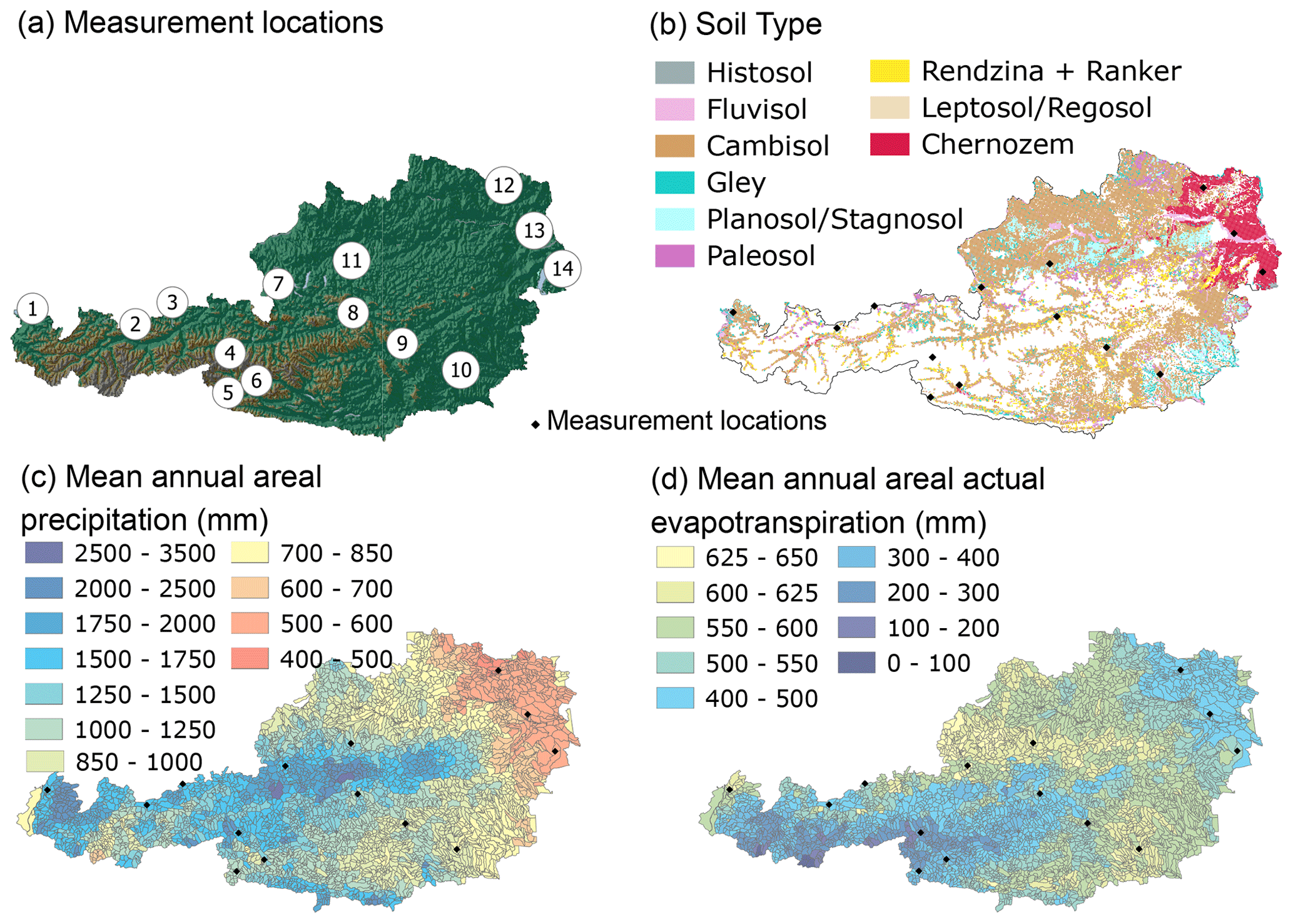
Figure 1Panel (a) outlines the locations of the following 14 monitoring sites in Austria: (1) Lauterach, (2) Leutasch, (3) Achenkirch, (4) Gschlössboden, (5) Sillianberger Alm, (6) Zettersfeld, (7) Elsbethen, (8) Gumpenstein, (9) Aichfeld-Murboden, (10) Kalsdorf, (11) Pettenbach, (12) Schalladorf, (13) Lobau, and (14) Frauenkirchen. Panel (b) provides the soil map data basis: digital soil map of Austria, 1 km raster, Federal Forest Research Center (BFW, 2016). Panel (c) shows the Hydrological Atlas of Austria (HAO) mean areal annual precipitation (Kling et al., 2007b), and panel (d) shows the HAO mean areal annual actual evapotranspiration (Kling et al., 2007a); maps from the HAO where compiled using QGIS (QGIS Development Team, 2022).
In this study, we made use of long-term volumetric soil water content measurements at 14 different locations from the Austria-wide soil water monitoring program and integrated them in a Bayesian probabilistic framework with the MultiNest algorithm to calibrate the HYDRUS-1D hydrological model at each location. We used this approach to account for the uncertainties inherently associated with the inverse parameter estimation, and we simultaneously assessed and propagated the model predictive uncertainty in simulated local potential groundwater recharge rates. All sites were modeled with the same approach on a similar data basis, supporting comparability of the results. Site properties included a variety of soils and climatic conditions, allowing for the investigation of factors that influence the long-term soil water balances and temporal variability in potential groundwater recharge.
2.1 Austrian soil water monitoring program
The locations of 14 Austrian soil water monitoring sites are shown in Fig. 1a. Figure 1b gives an overview of soil types according to the digital soil map of Austria (BFW, 2016). Figure 1c and d show the respective long-term annual areal precipitation (modified from Kling et al., 2007b) and actual evapotranspiration (modified from Kling et al., 2007a) estimates. According to texture information (ÖNORM L 1050, 2016), the soil types at the measurement sites vary between sand and silt loam/loamy silt (11 %–88 % sand, 12 %–75 % silt, and 0 %–32 % clay). Details on altitude, geo-coordinates, soil textures, and measurement depths are given in the Appendix (Table A1). Briefly, Zettersfeld, Gschlössboden, and Sillianberger Alm are on the subalpine level in the southwest of Austria, characterized by high organic matter contents, a coarse soil texture, and/or a high skeleton fraction; Leutasch, Achenkirch, Gumpenstein, and Aichfeld-Murboden are located on the montane level from western to central Austria, with soil textures ranging between sand and loam; Pettenbach, Elsbethen, and Lauterach are located in the foothill zone in western to central Austria, with soil textures ranging from loam to loamy silt; and Kalsdorf, Schalladorf, Lobau, and Frauenkirchen are situated in the southern and eastern lowlands, with sandy to loamy soil textures. Locations included in this study are horizontally even at the plot scale and usually consist of uncultivated grassland. In contrast, the cultivation of alternating crops was carried out at the Pettenbach location, and details regarding the crop cover at this site for calibration and validation periods were obtained from technical reports provided by the Upper Austrian Government (Land OÖ, 2013, 2014).
Long-term field measurements of volumetric soil water content, measured with time domain reflectometry/frequency domain reflectometry (TDR/FDR) over several years, partly since 1996, are carried out within the Austrian soil water monitoring program of the Federal Ministry of Agriculture, Forestry, Regions and Water Management (BML). Within the framework of this program, continuous measurements are conducted at various depth levels of soil profiles with the aim of providing standardized and quality-assured measurement data. In this study, for inverse parameter estimation, we selected calibration periods of around 6 months with sufficiently complete and plausible soil water content measurement series (Fig. A2) and aggregated the data to a daily resolution. We used a model spin-up period of 2 months to relax the effect of initial conditions on the estimation procedure. The length of calibration periods was chosen to be similar for all sites and was long enough to be informative for a range of soil water conditions. We excluded the winter season, which requires the simulation of snow accumulation and melt processes, as it increases the computational cost and numerical sensitivity of the simulations and introduces additional complexity and potential biases in the calibration. The use of spring–summer months, which have an alternation of wet–dry periods, is expected to increase the informativeness of soil water measurements. The monitoring program also offers composite matric potential measurements from tensiometers and gypsum blocks; however, the discontinuity of these data complicates the modeling and analysis, which is why they have not been used in this study. Validation periods were chosen to provide 1 year or more of continuous, plausible data. Snow hydrology was simulated for the model validation, as described in Sect. 2.2.1. Details on the calibration and validation periods are summarized in Table A2. Several locations were equipped with lysimeters: at Leutasch and Pettenbach, in situ soil water content measurements were directly obtained from lysimeter setups; in Gumpenstein, soil water content measurements were obtained from a soil profile next to a lysimeter cluster that provided long-term seepage measurements. Lysimeter measurements from Leutasch and Gumpenstein were used for additional validation of recharge rates.
2.2 Modeling theory
2.2.1 Water flow and root water uptake
The mechanistic HYDRUS-1D model (Šimůnek et al., 2016) was used to simulate water flow in the vadose zone profiles. HYDRUS-1D is a finite element model that numerically solves the one-dimensional Richards equation:
where θ (L3 L−3) is the volumetric water content, t (T) is the time variable, z (L) is a vertical coordinate, K(h) (L T−1) is the unsaturated hydraulic conductivity function, and h(L) is the pressure head. S (T−1) is a sink term accounting for water uptake by plant roots. The unimodal van Genuchten–Mualem (VGM) model describes the soil hydraulic properties, namely the soil water retention curve (Eq. 2), and the unsaturated hydraulic conductivity (Eq. 3).
Here, θr (L3 L−3) is the residual water content; θs (L3 L−3) is the saturated water content; α (L−1), n (–), and m (–) are van-Genuchten shape parameters, with the relation given in Eq. (4); Se (–) is the effective saturation (defined in Eq. 5); and l (L) is a pore connectivity parameter. The unimodal VGM model has successfully been used in several studies to parameterize the hydraulic behavior of variably saturated soils (e.g., Brunetti et al., 2020b; Dettmann et al., 2014; Lambot et al., 2002). It has been shown to become more inconsistent in the clay range of soil textures (Fuentes et al., 1992); however, this limitation does not affect any soils in the framework of this study, and the model was thus employed for all sites. The sink term for the simulation of plant water uptake is implemented as follows (Feddes et al., 1978):
where rd (L) is the root depth, Tp (L) is the potential transpiration, and α(h) is a prescribed water stress response function depending on the crop type. The crop parameterization for the sites in this study used the default values for grass cover (Taylor and Ashcroft, 1972), except for the Pettenbach calibration which used a maize parameterization according to Wesseling et al. (1991).
The model domain was set up from the soil surface to 1.5 m depth at all sites, and two different soil materials were defined for the upper soil (including 20 cm root zone) and the lower soil, respectively. The depths of the soil layers are given in Table A3. The available soil water measurements and profile information (texture data and soil horizons) indicated a distinct topsoil overlying deeper soil layers with low to mild degrees of inhomogeneity in the vast majority of the soil profiles. Dealing with 14 monitoring stations, we uniformly adopted two soil layers with varying thickness across different locations, aiming to reduce the overall computational burden of the Bayesian analysis while maintaining a physically realistic description of the soil domain. Simplifications of the soil profile in the model geometry with a mildly heterogeneous soil will usually lead to an acceptably small loss of accuracy in effective parameters (Schneider et al., 2013).
In this study, we define the point at which percolating water is expected to contribute to groundwater recharge as the amount of water that arrives at the bottom of the area at a depth of 150 cm, well below the root zone. It is assumed that water arriving at this depth will not be subject to further loss mechanisms and, therefore, will reach the water table (Heppner et al., 2007). Similar to our approach, Šimůnek (2015) and Heppner et al. (2007) simulated groundwater recharge with HYDRUS-1D for grass-covered soils as the bottom flux at a 100 cm profile depth; Assefa and Woodbury (2013) used different profile depths of up to 150 cm. However, as the point where water actually reaches the water table remains unknown, the estimation obtained using this approach can be referred to as potential recharge (Scanlon et al., 2002).
Daily time steps were used in all simulations, for variable boundary conditions and for simulated soil water content and water fluxes. Meteorological data for the sites, including precipitation, solar radiation, sunshine duration, wind speed, and relative humidity, were obtained from the Central Institution for Meteorology and Geodynamics (ZAMG), Austria. The potential evapotranspiration ET0 was calculated using the Food and Agriculture Organization (FAO) Penman–Monteith method, according to Allen et al. (1998). At the upper boundary of the model domain, an “atmospheric”, “zero-ponding” boundary condition was specified; to specify this boundary condition, an equilibrium is prescribed between the soil surface pressure and atmospheric water vapor pressure when the evaporative demand exceeds the soil evaporation capacity, and the pressure at the soil surface is set to zero when both infiltration and surface runoff occur. For the parameter estimation during the half-year calibration periods, as well as for the model validation periods, we chose boundary conditions with respect to the conditions at the measurement plots, i.e., seepage face for the lysimeter sites and free drainage for sites with natural field conditions. For the simulation of long-term potential recharge rates, the lower boundary condition at all sites was set to free drainage in order to reflect natural conditions with a water table far below the model domain. To improve the comparability of long-term simulations at the sites, a grass reference was used with the calibrated Pettenbach model to simulate long-term groundwater recharge. Long-term simulations comprised the entire period of available soil water and meteorological data. For the Achenkirch location, only 2 years of meteorological data (2017–2018) were available.
For model validation and long-term simulations, snow accumulation and snowmelt were accounted for in HYDRUS-1D. The model treats any precipitation falling at a temperature below −2 ∘C as snow and any precipitation above +2 ∘C as liquid, assuming a linear transition between −2 and +2 ∘C. A 0.4 factor as snow sublimation constant was used for the reduction of potential evaporation from snow, and the simulation of snowmelt at temperatures above 0 ∘C used a constant of 0.43 cm d−1 ∘C−1. This default snow routine in HYDRUS is based on assumptions by Jarvis (1994) and has been found to be suitable for estimating soil water fluxes in unfrozen soils in several studies (e.g., Assefa and Woodbury, 2013; Zhao et al., 2008).
2.2.2 Bayesian analysis
Bayes' theorem (Eq. 7) is the basis for the estimation of parameter posterior distributions, which are used for quantification of model parameter uncertainties after calibration.
Here, is the posterior probability of the model parameters (Ω), given the data (D) and the model (M); is the conditional probability of the data given the model and parameters; P(Ω|M) is the prior probability; and P(D|M) is the marginal likelihood or Bayesian model evidence (BME). Prior knowledge, i.e., information available before looking at measured data, is included in the Bayesian inference via the prior distribution, which can be chosen as a uniform density bounded by physical limits (e.g., Brunetti et al., 2020b; Gupta et al., 2022; Wöhling et al., 2015). In this study, uniform prior distributions were assumed for all parameters and sites. Their ranges were established based on texture information, literature review, and preliminary testing to prevent truncating posteriors. Final ranges are given in Table A3. By combining the likelihood and the prior, we obtain a posterior distribution of the most probable SHP values, which reflects the parameters’ uncertainty.
We used volumetric water content measurements from TDR sensors in the calibration; the measurement error is based on electromagnetic instantaneous pulses and can be assumed to be independent, homoscedastic, and normally distributed. This leads to a Gaussian likelihood function (Eq. 8), where σ is the standard deviation in the measurement error, Mi(Ω) is the model realization, and is the corresponding observed data:
The choice of likelihood function is critical to the outcome of Bayesian inference and is the subject of ongoing debate. A recent promising approach that should be explored in future studies is the universal likelihood approach proposed by Vrugt et al. (2022). Instead of making prior assumptions about the distribution of model residuals in the likelihood function, this approach is distribution-adaptive with respect to the actual residual properties. However, in the present study, we used the Gaussian likelihood function, as described above, for process-based probabilistic inference, and we employ significant, systematic discrepancies between model predictions and observations that violate our assumptions as indicators that the model structure needs improvement. We show the residual checks for the Gumpenstein location as an example in the Appendix (Fig. A1).
At all 14 locations, 10 soil hydraulic parameters (SHPs) (residual, θr, and saturated, θs, water content parameters, shape parameters α and n, and the saturated hydraulic conductivity parameter Ks, for two soil layers, respectively) were estimated per site. The pore connectivity parameter l was fixed to 0.5 according to Mualem (1976). Along with the SHPs, the standard deviations of the measurement errors were estimated in the Bayesian inference.
The implementation of the Bayesian approach in a numerical framework can become challenging for nonlinear models, such as the model used here. The nested sampling algorithm, as proposed by Skilling (2006), has been used successfully for parameter estimation and uncertainty quantification in studies with nonlinear hydrological or biogeochemical models (Brunetti et al., 2020a; Elsheikh et al., 2013). It has been tested in Schül et al. (2022) with synthetic data scenarios for SHP estimation with similar HYDRUS models and has been found to reliably infer the true parameter values as well as the standard deviations of the artificial errors in the calibration data. Nested sampling is an efficient Monte Carlo method that estimates the Bayesian model evidence and calculates posterior distributions as a side product. It transforms the multidimensional integral of the Bayesian model evidence (BME) into a one-dimensional one, which is then solved iteratively, based on the evaluation and redistribution of a number of “live points” over the parameter space. Several improvements were implemented with respect to the original algorithm, such as the ellipsoidal rejection sampling scheme which is able to establish multiple posterior modes. This has been realized in the MultiNest algorithm by Feroz et al. (2009). This algorithm has been shown to be well suited to multimodal distributions and moderately complex inverse problems with up to 20 parameters (Buchner, 2016; Feroz and Hobson, 2008). The algorithm is particularly suitable for our study because it offers a high level of efficiency for unimodal problems while also handling the possibility of multimodal posteriors. Further details on the algorithm can be found in Feroz et al. (2019, 2009), Feroz and Hobson (2008), and Mukherjee et al. (2006).
Here, we used a number of live points N=100 to sample the parameter space. This number has been shown to produce a reliable estimate of the BME integral (and therefore a satisfactory sampling of the parameter space) in a sensitivity analysis by Brunetti et al. (2020a, b) for similar models and dimensionalities. At each iteration of the algorithm, the current maximum likelihood sample point is multiplied by the remaining prior volume to estimate the maximum remaining volume of the BME integral. Sampling is then terminated according to a tolerance (convergence) criterion, which defines when the remaining contribution from the current live points to the integral is considered to be small enough. At this point, it is expected that the bulk of the posterior has been sampled sufficiently. The tolerance parameter in this study was set to 0.5. The number of posterior samples provided by MultiNest depends on the algorithm convergence with each model. On average, we obtained 4100 posterior samples and corresponding sample weights to characterize posterior parameter distributions. We used 100 random samples from the posterior to propagate parameter uncertainty in the model for long-term simulations in order to quantify the resulting uncertainty in recharge simulations. Uncertainty ranges for SHPs and soil water fluxes are given as 95 % interquantile ranges (IQRs).
2.2.3 Statistical analysis
Simulations with the successfully calibrated models were used in a second step to perform a statistical analysis in order to characterize and describe the variability in groundwater recharge at the monitoring sites and to assess the influence of climatic, geographic, and soil properties on potential groundwater recharge rates and their temporal variability. For this purpose, we used a principle component analysis (PCA) and established clusters of sites with similar properties using agglomerative clustering (Pedregosa et al., 2011). In order to quantify the temporal variability in water balance components, we calculated the coefficient of variation (CV) values, defined as the quotient of standard deviations between months within a year, as measure for seasonal variability. Spearman's ρ correlations were used to identify predictor variables for potential groundwater recharge rates and temporal variability. The significance of correlations was evaluated at a 90 % confidence level (p<0.1).
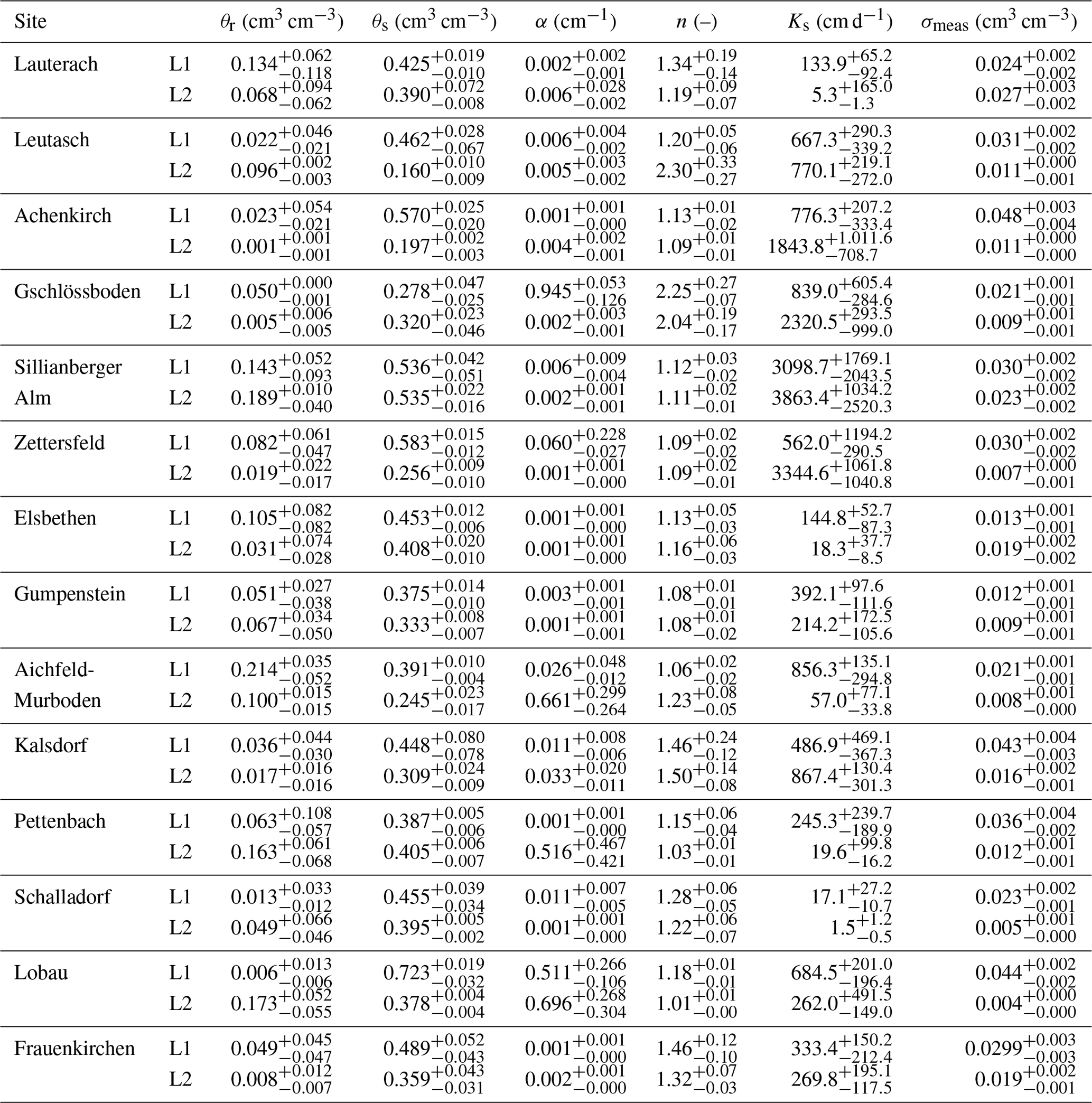
Table 1Median estimates and the 95 % credible interval of soil hydraulic parameters and measurement errors for the upper (L1) and lower (L2) soil profiles.
3.1 Calibration and validation
The required number of iterations of the MultiNest algorithm with models for all 14 locations ranged between 2595 and 5515 (4111 on average) until the termination criterion was satisfied (as described in Sect. 2.2.2), generally resulting in unimodal posterior parameter distributions. Median parameter estimates and estimated measurement errors including the 95 % credible interval are given in Table 1 for the upper and lower soil layers at the 14 sites. Figure 2 shows the calibrated measurement error and median prediction of the volumetric soil water content for the upper and lower soil layers for the Gumpenstein location as an example. Calibration plots for all 14 sites are shown in Fig. A2. In Fig. 3, the uncertainty in the parameter estimation is summarized for all 14 sites as ratios between the 95 % interquantile range (IQR) and the median estimate.
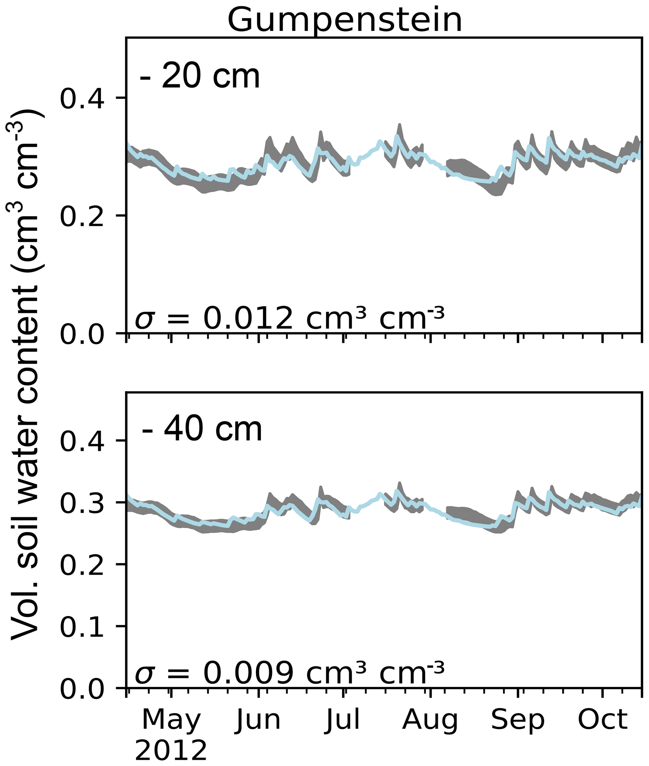
Figure 2Parameter estimation at Gumpenstein: calibration period with soil water content measurements (gray) from two depth levels, including the calibrated measurement error σ, and prediction with median parameter estimates (blue).
Median estimates for the VGM shape parameters α and n varied between 0.001 and 0.945 cm−1 and between 1.01 and 2.30, respectively, but α was <0.01 cm−1 at most sites. Except for the high α estimates at Gschlössboden (α1=0.945 cm−1) and Lobau (α1=0.511 cm−1 and α2=0.696 cm−1), the VGM shape parameters fell well within the range of values predicted by the ROSETTA pedotransfer model (Schaap and Leij, 1998); high estimates for α and n coincided with a high reported sand fraction. Median estimates for hydraulic conductivity parameters Ks ranged from 5 to 3863 cm d−1, and high values were found for soils with high organic and stone content fractions (Gschlössboden, Sillianberger Alm, and Zettersfeld).
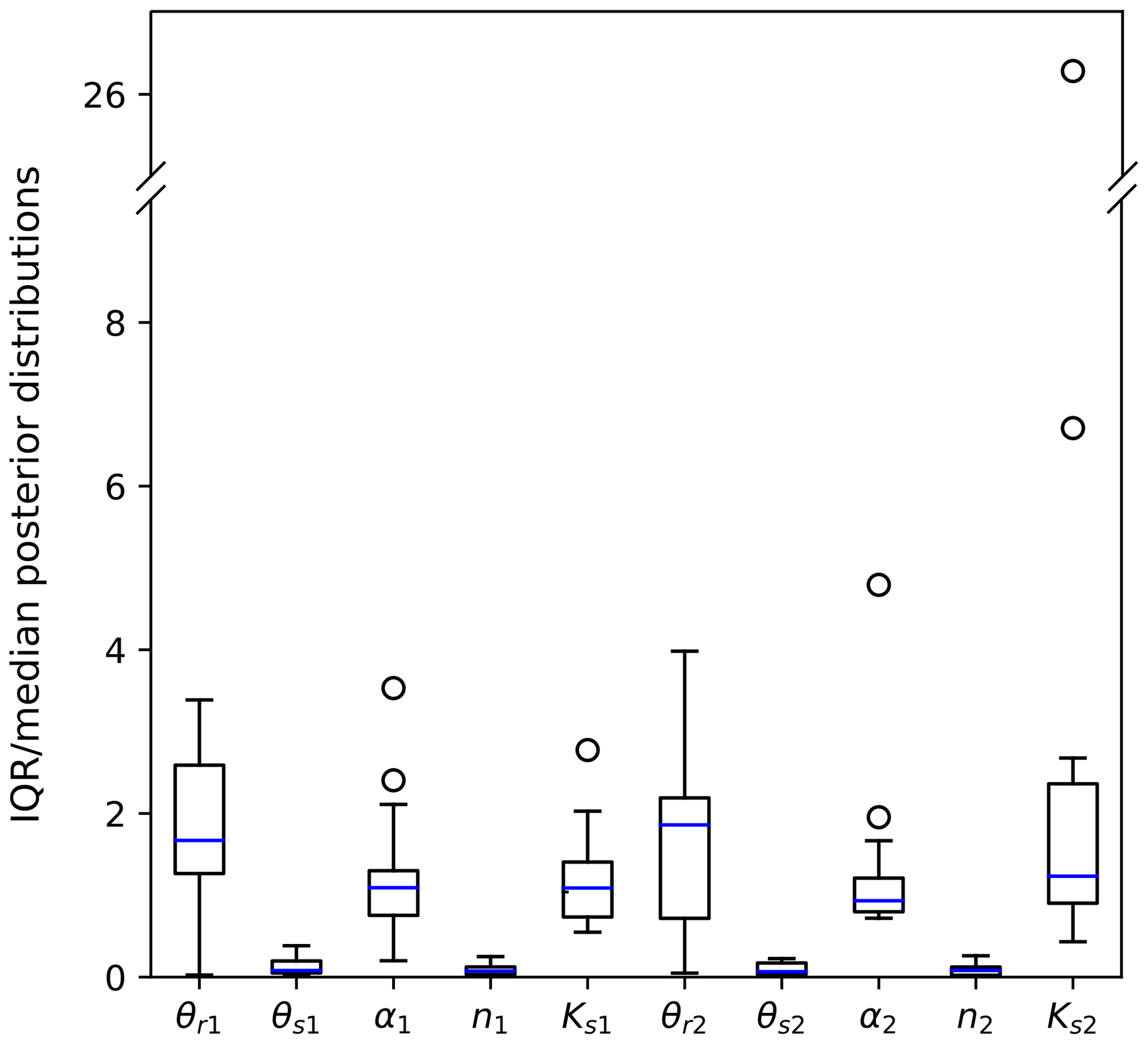
Figure 3Box plots of estimated parameter uncertainties (index 1 denotes the upper soil layer and index 2 denotes the lower soil layer) from all 14 sites, as ratios between the 95 % interquantile range (IQR) and median estimates.
A typical example of marginal posterior distributions resulting from SHP estimation on the basis of volumetric soil water content data in this study is shown in Fig. 4 for the upper soil layer of the mountainous Zettersfeld location. Limits of the plot axes are given by the prior bounds. This representation shows how well the calibration data constrained uncertainties in each parameter: the posterior range of θr is only slightly reduced compared to the prior range, indicating that θr was the least sensitive with respect to simulating soil water content and poorly informed by observations. The parameter Ks has a wide posterior range (although clearly reduced compared with the prior), showing a logarithmic distribution and a clearly defined mode. On the other hand, the parameters α and, especially, n and θs show narrow posterior distributions which appear leptokurtic, indicating a higher sensitivity for the soil water content simulations and a high information gain from the calibration data.
Parameter interdependencies in the inverse estimation are reflected in the shapes of the bivariate contour or scatterplots of posteriors (see Fig. A3 for a representation of posteriors with closer axis ranges). By random sampling from the posterior, the effect of these correlations is propagated in the uncertainty in the prediction of soil water fluxes. Usually, a negative relation exists between the VGM shape parameters (e.g., Scharnagl et al., 2011; Vrugt et al., 2003; Romano and Santini, 1999). Here, both α and n show narrow posteriors and stray close to the lower physical bounds (0 and 1, respectively). The correlation of posterior samples for α and Ks can be expected to have some effect on the uncertainty in recharge peak prediction, for which both parameters (but especially Ks under wet conditions) are sensitive (Schül et al., 2022). This will be further discussed in Sect. 3.2.
Generally, uncertainties in the estimation of the residual water content parameter θr and the saturated hydraulic conductivity parameter Ks for the sites were high, for both the upper and lower soil layers (IQR median ∼ 26 for Ks2 at Lauterach). The uncertainty in the shape parameter α was medium with a relative uncertainty (IQR median) < 6 and mostly low absolute values for the estimates and uncertainty ranges. The shape parameter n and the saturated water content parameter θs were identified with the highest precision (IQR median < 0.5).
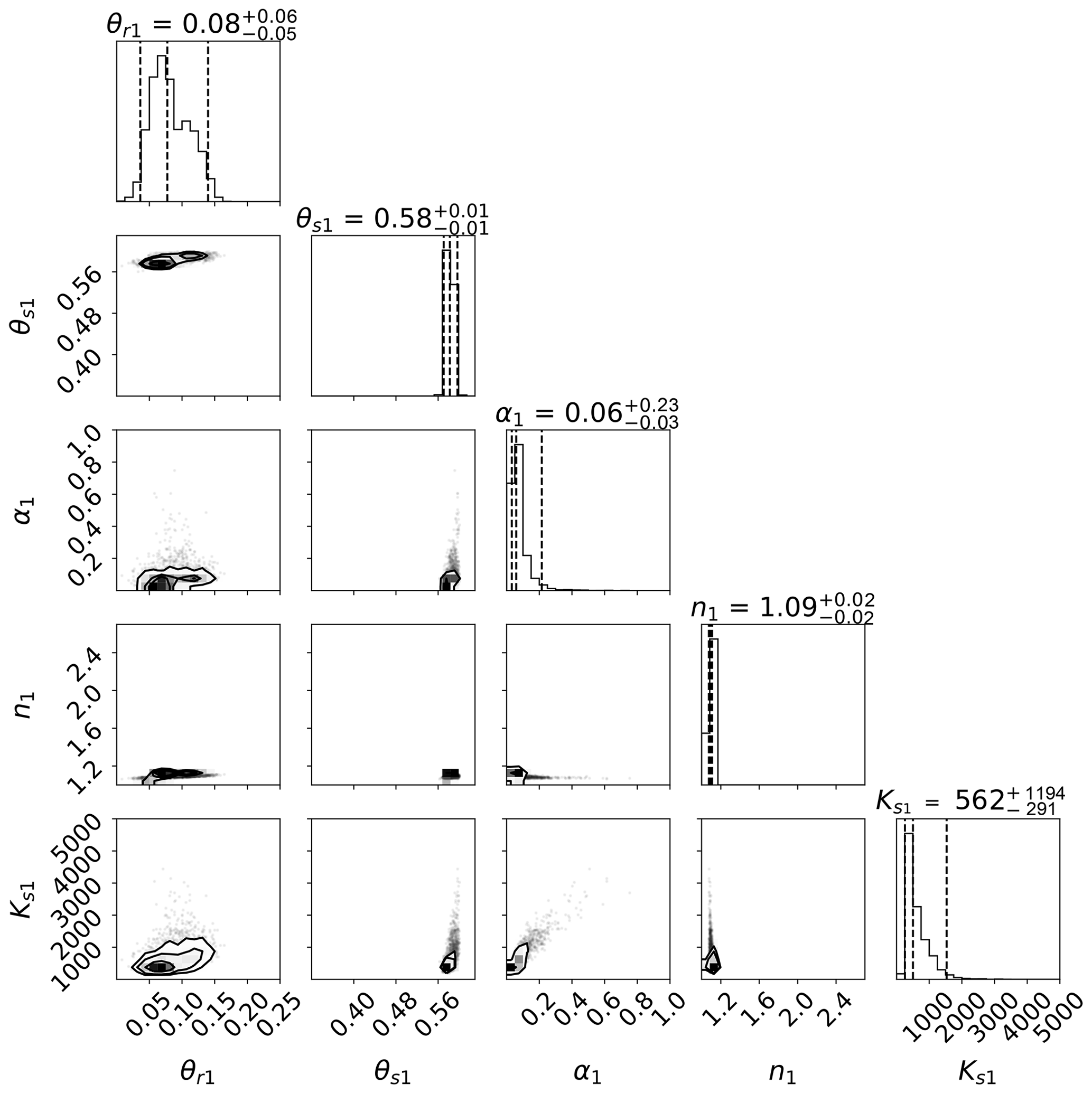
Figure 4Marginal posterior distributions (one-dimensional projection on top of each column and joint distributions of each two parameters below) of estimated SHPs for the upper soil layer at Zettersfeld. Presented are the respective residual and saturated water content parameters θr and θs (cm3 cm−3), the VGM shape parameters α (cm−1) and n (–), and the saturated hydraulic conductivity parameter Ks (cm d−1). The axis ranges correspond to the parameter bounds of the prior distribution. A close-up presentation of distributions with narrower axis ranges is shown in Fig. A3.
Overall, SHP estimation using soil water content monitoring data from different depth levels was associated with some uncertainty. An important factor for parameter uncertainty was soil texture: uncertainties in the Ks and n parameters, in terms of the 95 % interquantile range (IQR) for posteriors, were significantly positively correlated with the percentage of sand (r=0.43 and r=0.42, respectively). Uncertainty ranges in Ks, α, and n increased significantly with the value of median estimates (Fig. 5). Higher values of these parameters signify a lower water retention capacity of the soil. According to results from Schül et al. (2022) and Gao et al. (2019), parameter uncertainty from calibration with daily soil water content measurements can be expected to be higher in coarse-textured soils (with a higher soil hydraulic conductivity and lower soil water retention capacity) than in fine-textured soils – which was the case in this study. We suppose that the more rapid water flow processes are less efficiently captured in daily soil water content measurements, which are consequently less efficient with respect to constraining the uncertainties in SHPs.
We expectedly found high parameter uncertainties for sites where the estimated errors were high (σ>0.04 cm3 cm−3 at Kalsdorf and Lobau) or where the error was high in comparison to the temporal variation (more than 90 % of the standard deviation in the observations at Zettersfeld and Sillianberger Alm). Xie et al. (2018) observed how the relation between the size of the estimated measurement error and the temporal variation in the measured variable influences the ability of the data to constrain model uncertainties. In the estimation of SHPs with remote sensing soil moisture data, Brunetti et al. (2019) observed that uncertainty in θr estimation was low, whereas θs was highly uncertain. This was related to soil water content values being low in their study and mainly representative of unsaturated conditions. In this study, at Lauterach and Elsbethen, very wet climatic conditions and measurements mainly in the wet range resulted in the highest uncertainties in the estimation of θr. At Kalsdorf, in contrast, soil moisture dynamics were hardly at saturation and resulted in the highest uncertainty in θs estimation. At the majority of the Austrian locations, soil water content measurements were more often near saturation and less in the dry range (as, for example, at Gumpenstein in Fig. 2a). The θs parameter was, therefore, mostly better informed by the measurements than θr. The estimation of Ks has been frequently shown to be associated with high uncertainties (e.g., Baroni et al., 2010; Minasny and Field, 2005; Mishra et al., 1989).
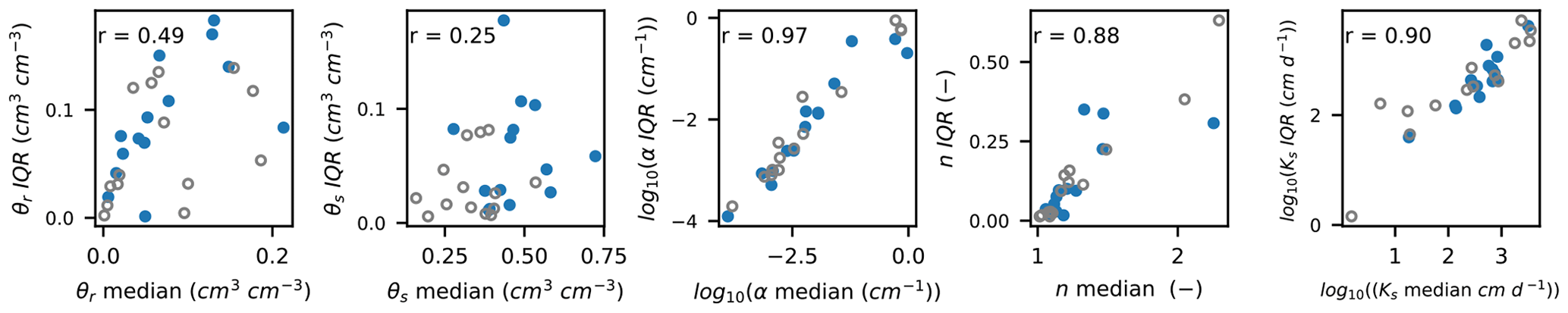
Figure 5Correlations between median parameter estimates and the 95 % interquantile range (IQR) from posterior parameter distributions for estimated SHPs for 14 sites – each with two soil layers (blue dots show the upper soil layer and gray circles show the lower soil layer). The α and Ks parameters are shown on a log scale to better depict the range of values. Spearman's ρ (r) is given for the presented correlations. The correlations were highly significant with p<0.01 for α, n, and Ks on a log scale as well as on a linear scale. On the linear scale, r was slightly lower for α (r=0.77) and Ks (r=0.89).
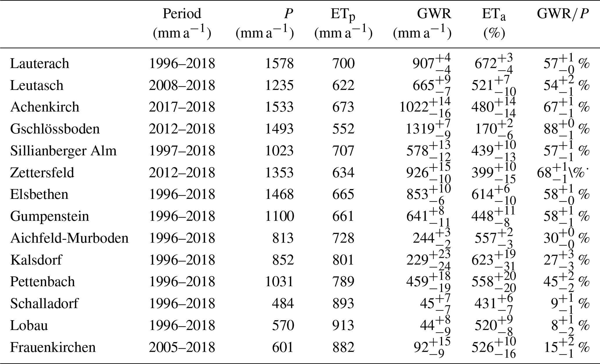
Table 2Local long-term average water balances at 14 sites, showing precipitation (P), potential evapotranspiration (ETp), and the simulated potential groundwater recharge (GWR) and actual evapotranspiration (ETa) with the 95 % credible interval from propagated parameter uncertainty.
The reliability of the calibration was quantified by the root-mean-square error (RMSE) between median simulations and observations during calibration and validation periods (summarized for all sites in Table A2). Overall, the calibration fit was good, with RMSE values ranging between 0.009 and 0.028 cm3 cm−3. Some events were missed by the model: at Lauterach and Elsbethen, the drying of the lower soil layer in summer was underestimated; at Gschlössboden, the peak in soil water content in the early calibration period was missed for both layers. For the validation periods, the fit in terms of the RMSE deteriorated, especially for the Lobau (calibration RMSE = 0.028 cm3 cm−3 and validation RMSE = 0.054 cm3 cm−3) and Pettenbach (calibration RMSE = 0.020 cm3 cm−3 and validation RMSE = 0.067 cm3 cm−3) locations. The Lobau soil profile was under the influence of water table fluctuations; thus, we cannot exclude that model assumptions about the lower boundary condition have been occasionally violated at this location. At the Pettenbach lysimeter station, crop rotation including fertilization was applied. It is possible that this affected soil properties, which were assumed to be constant in the modeling. For example, in their review, Lu et al. (2020) showed that root growth and decay can alter soil hydraulic properties; moreover, Whalley et al. (2005) found that growing different plants had a significant effect on the porosity of the soil aggregates, and Schjønning et al. (2002) observed the development different pore systems in soils depending on crop rotation and fertilization.
Overall, in the validation periods RMSE values ranged between 0.014 and 0.067 cm3 cm−3. Scatterplots including the coefficients of determination (R2, 0.34–0.98) for the validation period are shown in Fig. A4.
3.2 Simulated long-term water balance at the local scale
The calibrated models were used to simulate and assess different components of the water balance for all monitoring stations. In particular, we looked at long-term estimates and temporal variability in actual evapotranspiration and potential groundwater recharge as well as the average fractions of potential groundwater recharge from precipitation. Long-term averages of input and simulated annual water balance components including propagated parameter uncertainties are given in Table 2. Figure 6 shows cumulative potential recharge sums for the entire simulation period including propagated posterior uncertainty for all 14 sites; Fig. 7 shows the uncertainty in the peak prediction as maximum daily recharge rates and posterior uncertainty during the same period.
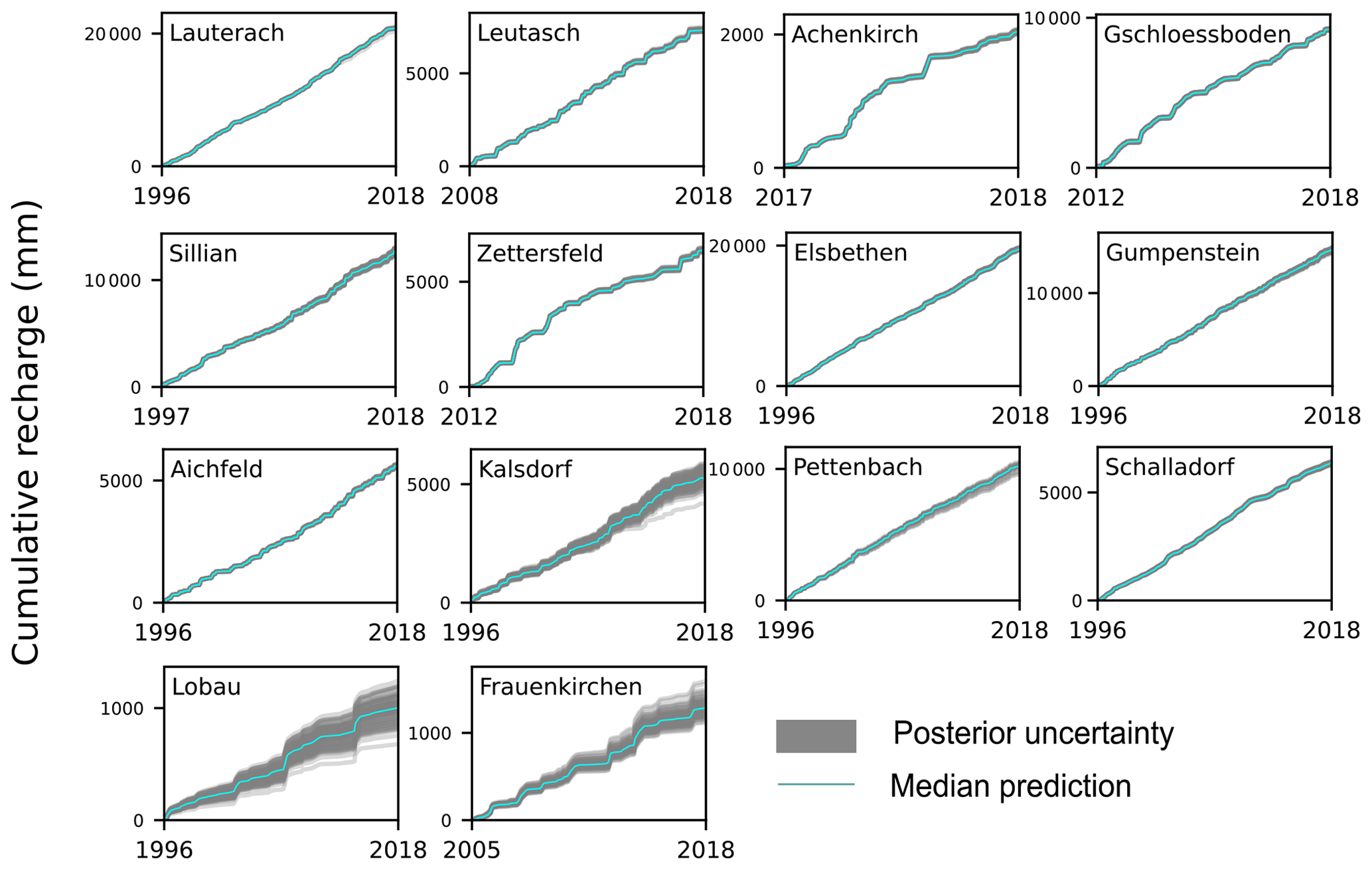
Figure 6Median prediction and posterior uncertainty in the long-term estimation of cumulative recharge at 14 Austrian sites.
Uncertainty in the estimated long-term potential annual recharge from propagated parameter uncertainty was highest in Kalsdorf (95 % IQR = 47 mm) and lowest in Aichfeld-Murboden (95 % IQR = 5 mm). Uncertainties in the prediction of long-term and cumulative recharge rates (Fig. 6) were generally small in relation to the high sums estimated for mountain and western sites; however, in relation to low absolute values at dry eastern sites (Kalsdorf, Lobau, and Frauenkirchen), posterior uncertainties played a more important role. The relative uncertainty (IQR median) in long-term recharge estimates ranged between 1 % (Gschlössboden and Lauterach) and 39 % (Lobau). The prediction of peaks in recharge was generally affected by higher uncertainties (Fig. 7), especially at western mountainous sites with high maximum rates (Lauterach, Leutasch, Gschlössboden, and Sillianberger Alm). In a previous study with similar models and hydrological conditions, we found n to be the most sensitive parameter for cumulative recharge prediction and Ks to be most sensitive for peak prediction, especially under wet climatic conditions (Schül et al., 2022). Small uncertainties in the prediction of long-term recharge sums here were related to the generally small uncertainties in the VGM shape parameter n, whereas higher uncertainties in the hydraulic conductivity parameter Ks (sometimes in combination with uncertainties in α) can be considered the main reason for the greater uncertainty in the peak prediction.
It has often been found that in situ field measurements of soil water content are not sufficient for the accurate and precise estimation of SHPs (e.g., Scharnagl et al., 2011; Ritter et al., 2003). Here, we found that while SHPs were partially affected by considerable uncertainties, the precision was still in an acceptable range for groundwater recharge estimation. At dry locations with small absolute recharge rates, model uncertainties could be further reduced by, e.g., including additional observations in the calibration. In particular, the combination with soil matric potential measurements has been shown to be highly informative for SHP estimation and to considerably reduce uncertainties in recharge estimation (Schül et al., 2022; Schelle et al., 2012). Including additional measurements in the analysis, however, might not only lead to different shapes in SHP posteriors but also to altogether different estimates. This issue requires further investigation with available soil water monitoring data.
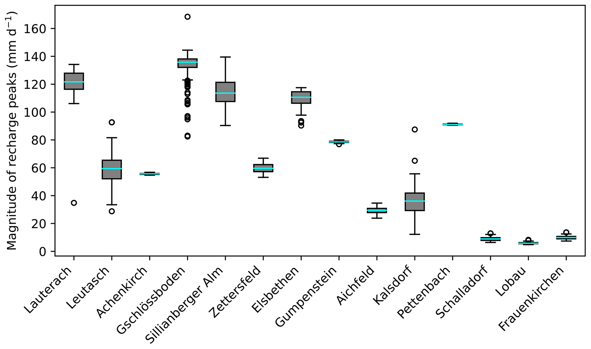
Figure 7Uncertainty ranges in peaks of the potential recharge flux at 14 Austrian sites. Maximum daily rates of the long-term simulation period and propagated posterior uncertainties are presented using box plots.
Propagated uncertainties in the soil water fluxes presented here are a result of parameter uncertainties from the calibration as well as of the sensitivity of the simulated water fluxes towards the parameters. Uncertainties in water fluxes were treated as aleatory and were derived from stationary statistical characteristics. In addition, the epistemic uncertainty associated with the lack of knowledge about the correct representation of system dynamics (conceptual uncertainty) and forcing data may affect the overall predictive uncertainty and reduce the effective information content of observations (Beven, 2016). Due to their complex and often dynamic nature, epistemic uncertainties pose important conceptual and numerical challenges. For instance, model conceptual uncertainty can be assessed by comparing different model structures using specific statistical metrics (e.g., marginal likelihood). This was, however, beyond the scope of the present study, which focuses on the inverse estimation of soil water fluxes at multiple monitoring stations to discuss the implications for the water balance. In this framework, an appraisal of the model structural adequacy through posterior predictive checks appears sufficient. In this work, we were not able to account for some processes that may have affected water balances at the sites: the modeling approach assumed that the groundwater table was well below the model domain at all times. At the Lobau site, however, the groundwater table is shallow, and fluctuations may have reached into the model domain. In this case, infiltrating water may have reached the water table earlier than assumed by the model. At the same time, net recharge would have been reduced if the capillary fringe extended into the root zone or even to the soil surface and transpiration and evaporation occurred directly from groundwater (Doble and Crosbie, 2017). Further, the modeling approach here neglected preferential and lateral flow processes. The ground surface at the measurement locations was even; however, it has been shown that heterogeneity and layering in the soil profiles can lead to lateral flow, even when the effective hydraulic gradient is vertical (Heilig et al., 2003; Rimon et al., 2007).
To assess the plausibility of estimated potential recharge rates, we compared them to literature values where available. Tóth et al. (2016) assumed annual groundwater recharge for the western Pannonian Basin of 70 mm a−1. The region includes the three southeasternmost sites here (Lobau, Frauenkirchen, and Kalsdorf), for which potential recharge rates in this study ranged between 44 and 229 mm a−1. For Wagna in southern Styria, 20 km from Kalsdorf, potential recharge rates of between 296 and 396 mm a−1 have been estimated in studies by Collenteur et al. (2021) and Stumpp et al. (2009). We also compared the estimates with the long-term (1961–1990) water balance averages for precipitation and potential and actual evapotranspiration at the catchment scale from the Hydrological Atlas of Austria (HAO) (BMLFUW, 2007; Dobesch, 2007; Kling et al., 2007b, a) (Fig. A5). The mean annual areal actual evapotranspiration estimates of the HAO (Kling et al., 2007a) are based on water balance calculations from the period from 1961 to 1990. They are comparable to our long-term estimates (R2=0.78), supporting the plausibility of the water balances established here.
We further evaluated estimated recharge rates at the Leutasch and Gumpenstein locations by comparing the available lysimeter outflow measurements to modeled median estimates. This resulted in an acceptable agreement with R2=0.56 (for the 2008–2018 period) and R2=0.64 (for the 2001–2018 period), respectively, and is shown in Fig. A6 in the Appendix, including uncertainties. Variability in annual seepage measurements between four Gumpenstein lysimeters was high, with an average uncertainty range of 132 mm a−1. This clearly exceeded the average range of predictive uncertainty related to the parameter uncertainty of the modeling at this site (20 mm a−1). Besides the uncertainty in the seepage measurement, the variability in the measurements could also be an indicator of spatial heterogeneities causing differences in the soil hydrology for individual lysimeters. In any case, the high variability in seepage measurements here emphasizes the need to analyze uncertainties in the estimation of soil water fluxes.
3.3 Statistical analysis of hydrologically relevant properties
In the following section, we characterize the 14 monitoring sites according to hydrologically relevant properties, including model estimations from the previous section. As uncertainty in long-term actual evapotranspiration and recharge rates was generally low and in order to enable the analysis with common statistical tools, we will use the median values without consideration of uncertainty ranges in the following.
The seasonal variability in groundwater recharge (quantified as the coefficient of variation from the standard deviation between monthly sums and annual means) ranged between 71 % and 265 %. This was consistently higher than the seasonality in precipitation (52 %–76 %) and potential evapotranspiration (64 %–76 %), indicating that potential recharge rates vary significantly more over the year than the meteorological input variables. We further analyzed the seasonality in local water balances using a PCA and correlation analysis. Figure 8 shows the biplot of the PCA with the first and second principle components (PC1 and PC2, respectively) explaining 77 % of the variance in the data, according to the amount and seasonality of water balance components, the fraction of potential groundwater recharge from precipitation, and site-specific properties (altitude and longitude as well as the sand, silt, clay, and organic matter percentages of the upper soil layers).
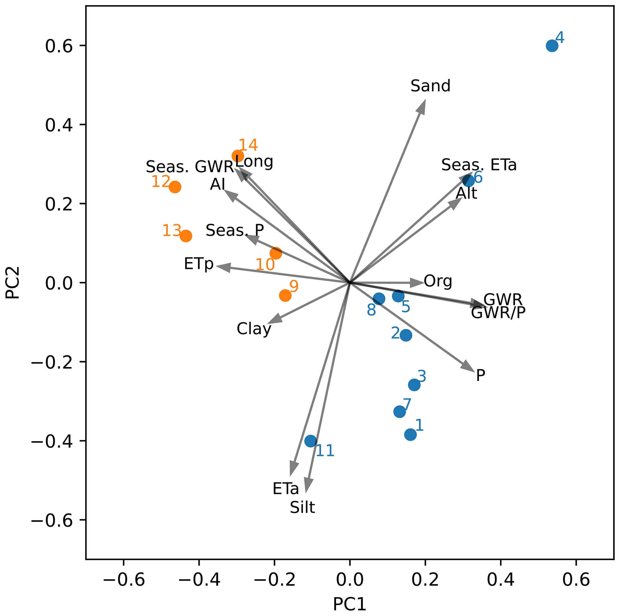
Figure 8A principle component analysis biplot for which the included variables at the 14 sites are as follows: potential annual groundwater recharge (GWR); annual precipitation (P); annual potential evapotranspiration (ETp); annual actual evapotranspiration (ETa); the fraction of groundwater from precipitation (GWR); seasonalities (Seas.) in GWR, P, and ETa; longitude (Long); altitude (Alt); and sand, silt, clay, and organic matter (Org) percentages. Clusters of monitoring sites with similar characteristics are shown in orange and blue. The clustering with Euclidean affinity and ward linkage as well as the biplot were produced using the Scikit-learn module of Pedregosa et al. (2011) in Python.
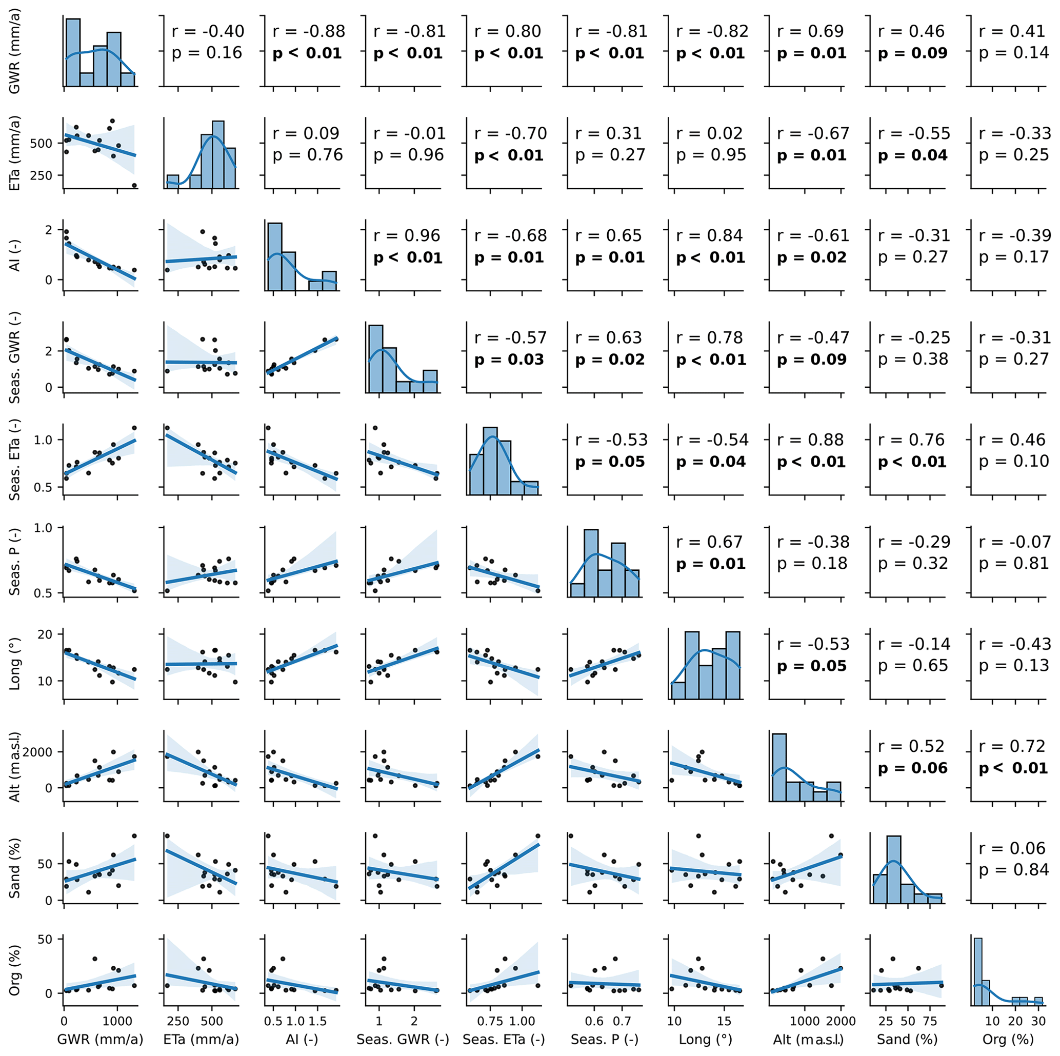
Figure 9Correlation analysis with pair-wise scatterplots, showing Spearman's ρ correlation coefficient and significance levels for the following variables at the 14 monitoring sites: potential annual groundwater recharge (GWR); annual actual evapotranspiration (ETa); the aridity index (AI); seasonalities (Seas.) in GWR, ETa, and P; longitude (Long); altitude (Alt); and the percentages of sand and organic matter (Org).
Two clusters were established: the five sites in the south and east of Austria – Aichfeld-Murboden (9), Kalsdorf (10), Schalladorf (12), Lobau (13), and Frauenkirchen (14) – show a potential recharge fraction of less than 30 % of annual precipitation (as low as 8 % in Lobau), a high seasonality in groundwater recharge (134 %–265 %) and precipitation (67 %–76 %), but a low seasonality in actual evapotranspiration (59 %–73 %). The remaining nine sites (of those used in this work) in western to central Austria with a humid to wet climate show a fraction of potential groundwater recharge from precipitation of more than 40 % as well as a low seasonality in precipitation (52 %–68 %). The seasonality in groundwater recharge at these sites was lower than in the east (71 %–124 %), but seasonality in actual evapotranspiration was higher (75 %–112 %); this was most pronounced at the three subalpine sites – Gschlössboden (4), Sillianberger Alm (5), and Zettersfeld (6) – which were influenced by snow and where little to no actual evapotranspiration was estimated outside of the extended summer period (May–September). An obvious outlier among the monitoring sites in Fig. 8a was Gschlössboden (4) at high altitude, which displayed coarse soil, the lowest potential and actual evapotranspiration, and the highest estimated potential recharge rates compared with other sites.
Figure 9 shows the pair-wise scatterplots, correlation coefficients, and significance levels of relevant variables. As precipitation and potential evapotranspiration were negatively correlated, we adopted the aridity index (ET) as a predictor instead of looking at both variables separately. Seasonality in potential evapotranspiration is not shown, as no significant correlations to other variables were identified. Soil texture grain size classes were intercorrelated; therefore, we only used the sand fraction as predictor variable.
Potential annual groundwater recharge rates were negatively correlated with aridity (lower precipitation and higher potential evapotranspiration). This was expected and was also supported by the findings of Moeck et al. (2020) at the global scale. At the Austrian sites, aridity increased and potential groundwater recharge decreased significantly with longitude, resulting in lower potential recharge rates for the eastern than for the western sites. Precipitation and recharge rates were higher in the west than in the east, following both the longitudinal gradient in altitude and the climatic influence of the wet oceanic climate in the west, with high precipitation and recharge rates even at lower altitudes (Lauterach and Elsbethen), versus the dry continental climate in the east. In this study, slopes were not taken into consideration, as the monitoring sites were horizontally even and the modeling domain was limited to the plot scale. Regarding the larger scale (and actual recharge rates), the occurrence of steep slopes at high altitudes would be expected to result in more surface runoff or more interflow instead of recharge (Brunetti et al., 2022; Moeck et al., 2020) which could reverse the correlation of recharge rates with altitude.
The fraction of potential groundwater recharge to precipitation (GWR) was strongly correlated with the amount of precipitation (r=0.91, p<0.001). Similarly, Barron et al. (2012) found an exponential relationship between annual recharge and rainfall estimates at Australian sites, which they explained by the correlation of high amounts of precipitation with high rainfall intensities and long wet periods throughout the year, leading to an increased fraction of recharge from precipitation.
Higher potential recharge rates and lower actual evapotranspiration were correlated with a higher percentage of sand. Soils with a greater sand fraction and less fine material have a higher hydraulic conductivity and a lower water retention capacity, as they let water percolate faster below the root zone (Emerson, 1995; Wohling et al., 2012). Wang et al. (2009) observed how the fraction of recharge from precipitation increased with coarser soil texture as the more rapid deep percolation reduced evapotranspiration. In this work, however, the relation between potential groundwater recharge and soil texture was weaker compared with climatic factors, i.e., precipitation and potential evapotranspiration. This corresponded to the findings of the global-scale analysis by Moeck et al. (2020).
Seasonality in potential groundwater recharge was most strongly correlated with the aridity index (ET). Sites in the east, which have more pronounced aridity and low potential recharge rates, were associated with a high seasonality with extended periods of zero recharge. Estimated potential groundwater recharge in these regions was concentrated in the winter half year. High rates of potential groundwater recharge were associated with sites where recharge occurred throughout the year and were, thus, correlated with low seasonality in recharge. Soil texture did not correlate with the seasonality in estimated potential groundwater recharge. In this study, we assumed the same lower boundary for all profiles to ensure comparability among the sites for which additional data from below 1.5 m were not available. However, the depth of the water table (and thus the thickness of the unsaturated zone) and structural features causing lateral flow determine the quantity and timing of water actually reaching the aquifer. With a greater thickness of the unsaturated zone, the influence of soil water retention characteristics on the magnitude and temporal variability of actual groundwater recharge rates might increase (Burri et al., 2019; Cao et al., 2016; Moeck et al., 2020). In future, data from the deeper unsaturated zone (>1.5 m) would be helpful to further improve the quantification of recharge.
In this study, we made use of volumetric soil water content measurements from multiple depth levels at 14 locations in Austria to inversely estimate effective soil hydraulic parameters (SHPs) using the physically based HYDRUS-1D model, and we quantified parameter uncertainties in a Bayesian probabilistic framework based on multimodal nested sampling. We used the calibrated models for the long-term simulation of soil water fluxes and associated uncertainties. Finally, we compared potential recharge rates and actual evapotranspiration at the 14 Austrian locations to identify the influencing factors on the amount and temporal variability of local water balances.
SHPs were successfully established and resulted in adequate fits of model simulations to observations. The parameter estimation based on soil water content measurements was partly subject to considerable uncertainties, especially with respect to the residual water content (θr) and soil hydraulic conductivity parameters (Ks). The latter resulted in considerable uncertainties in predicting the magnitude of recharge peaks at the sites. Higher uncertainties in the VGM shape parameters α and n and in the soil hydraulic conductivity parameter Ks were associated with coarser soil textures. In general, however, uncertainty in the estimation of the VGM shape parameters was low and resulted in small uncertainty ranges for long-term potential groundwater recharge rates. Absolute uncertainty ranges were between 5 and 47 mm a−1, which corresponded to relative uncertainties in cumulative recharge prediction (IQR median) of between 1 % (at sites with high absolute rates in a wet climate) and 39 % (at dry eastern sites with small potential recharge rates). Especially at the latter sites, model uncertainties could be improved by including additional observations in the calibration.
Estimated potential groundwater recharge rates at the Austrian soil water monitoring sites were influenced by the east–west gradient in altitude and climatic conditions: the dry continental climate at the eastern locations was associated with low potential groundwater recharge fractions from precipitation and with high seasonality in potential recharge rates. In contrast, the wet and snow-influenced climate at the western and central Austrian sites resulted in high potential recharge rates and lower temporal variability in recharge than in the east as well as a higher seasonality in actual evapotranspiration. Sandy soil textures were associated with higher potential recharge rates and lower actual evapotranspiration. However, precipitation and potential evapotranspiration were more influential variables than soil properties with respect to estimated potential recharge rates and their temporal variability.
The approach could be improved by including information on the deeper vadose zone to obtain more insight into temporal variation and seasonality of actual recharge and to improve the model structure, including lower boundary conditions. Especially at dry locations, using improved and additional measurements (e.g., of soil matric potential) could help reduce uncertainty in cumulative recharge estimation. Additionally, consideration of sites with varying slopes and the inclusion of surface runoff simulations in the analysis might improve representativeness at a larger scale.
Overall, the use of a nested-sampling-based Bayesian approach proved to be an efficient method to inversely estimate SHPs and soil water fluxes as well as to quantify associated uncertainties from soil water monitoring data. The calibrated models can be used to estimate future groundwater recharge rates under climate change and to illuminate model uncertainties resulting from SHP uncertainties and a range of climate scenarios.
Table A1Site properties and particle size distribution of the upper soil layer (ÖNORM L 1050, 2016).
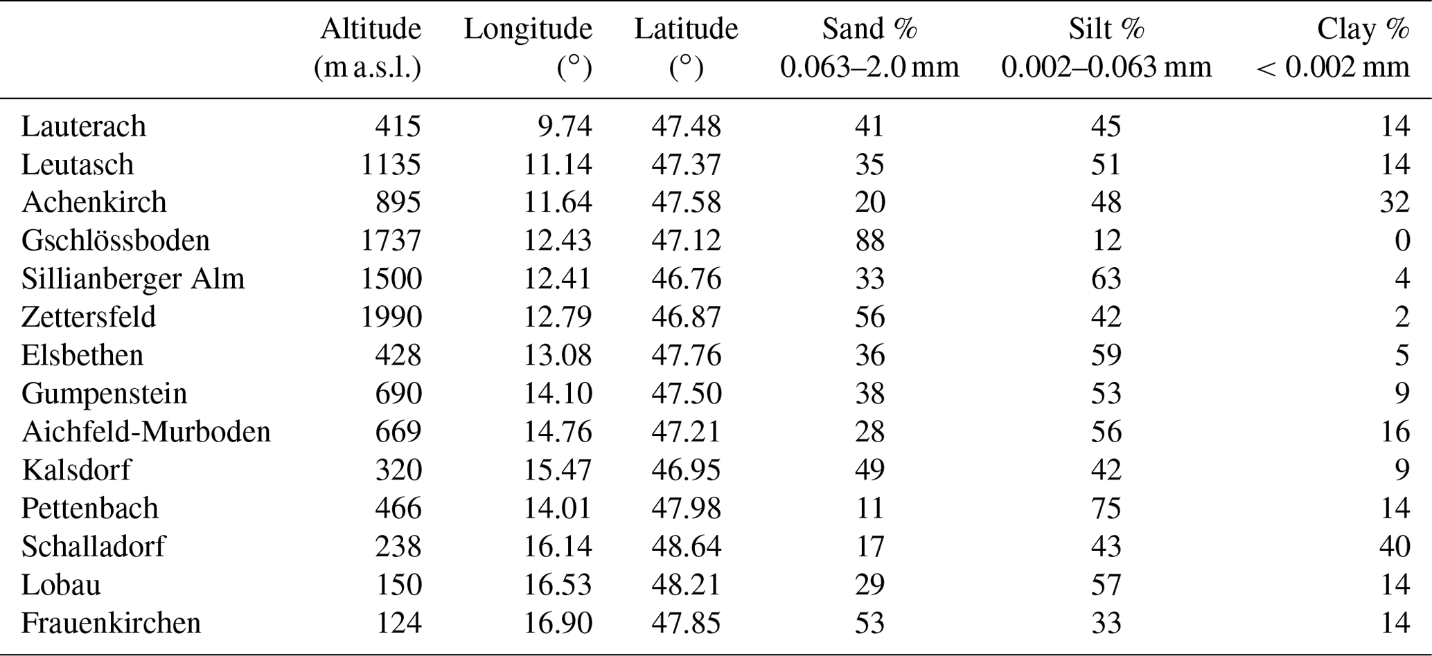
Table A2Calibration and validation periods, showing the goodness of fit (root-mean-square error, RMSE) between the median prediction and measurements.
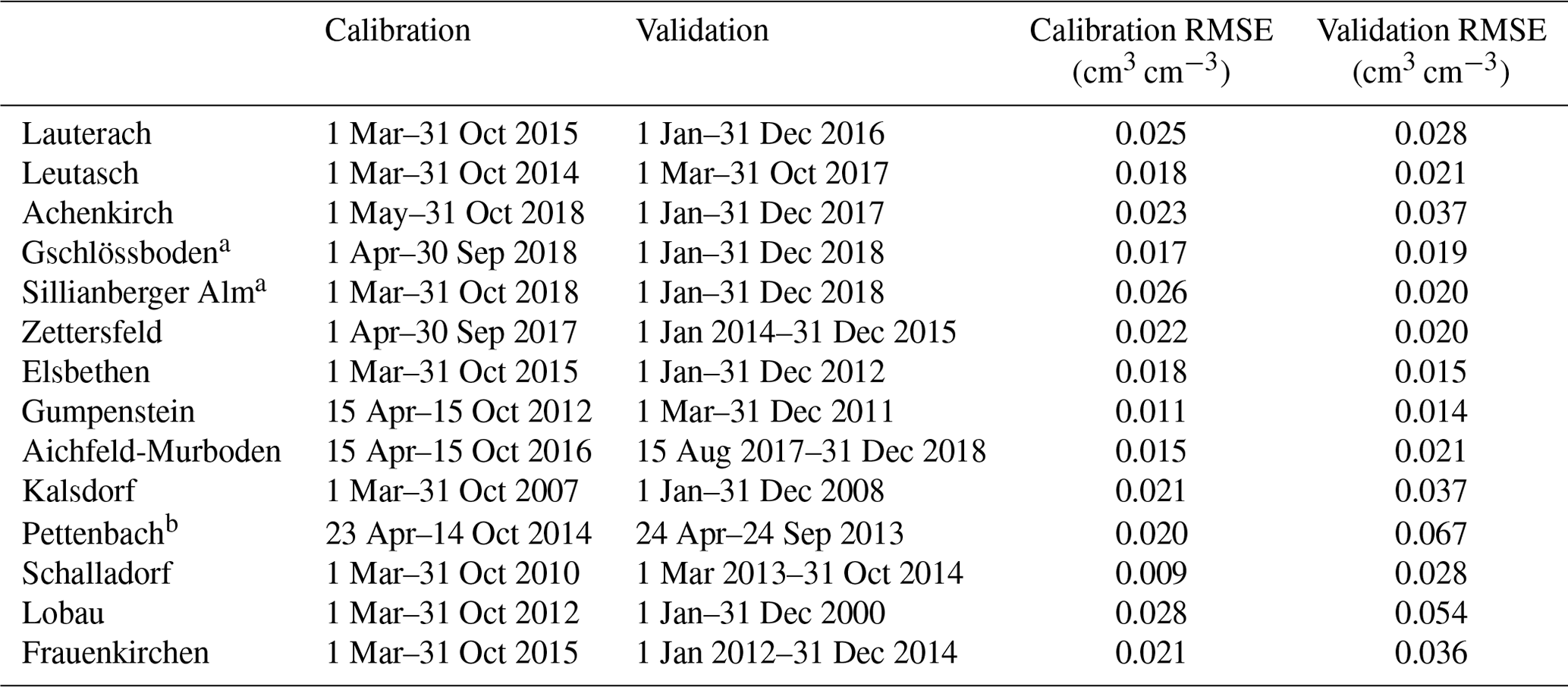
a No validation data are available outside the calibration year; instead, the RMSE for the entire year (2018) was calculated. b The Pettenbach calibration period was during maize cultivation and the validation period was during soy bean cultivation; root parameters were adjusted, and potential evapotranspiration estimation was estimated with the corresponding crop coefficients (Allen et al., 1998).
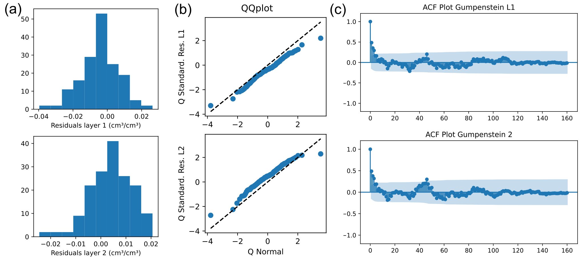
Figure A1Residual plots for the calibration at Gumpenstein: (a) histogram of residuals, (b) quantile–quantile (QQ) plots, and (c) autocorrelation function (ACF) plots. The upper graphs show residuals of the upper soil layer (L1) and the lower graphs show residuals of the lower soil layer (L2).
Table A3The soil layers in HYDRUS-1D and the prior parameter ranges of the Bayesian analysis.
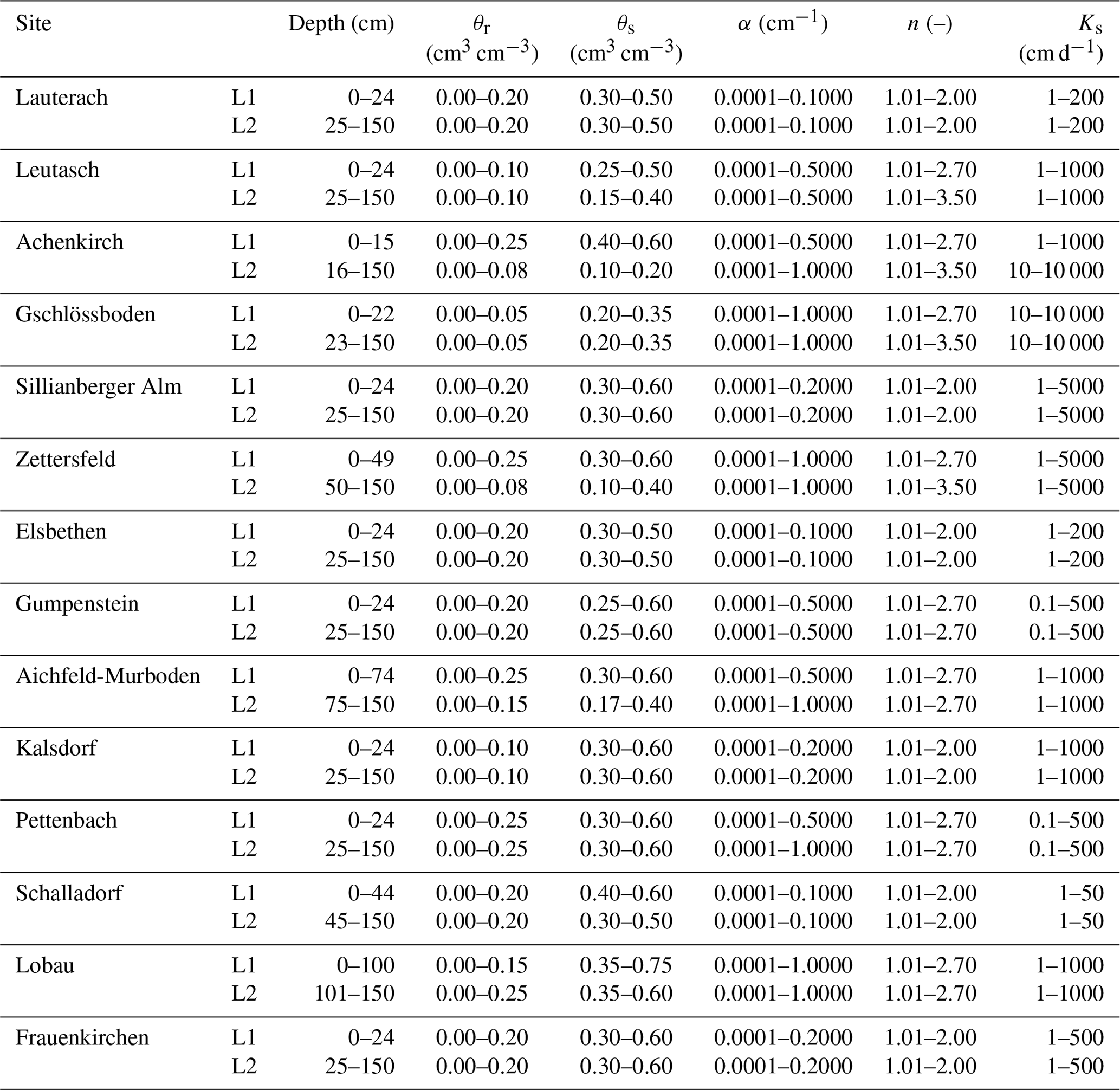
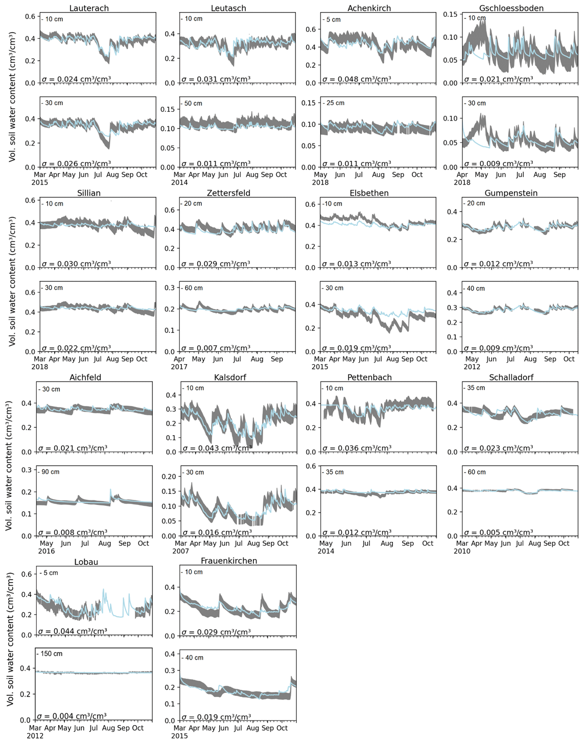
Figure A2Calibration with soil water content measurements at all 14 sites: the gray bands show the measurement, including the area of the calibrated measurement error σ, and the blue lines show the prediction with the median parameter estimates for each measurement depth in the upper and lower soil layer.
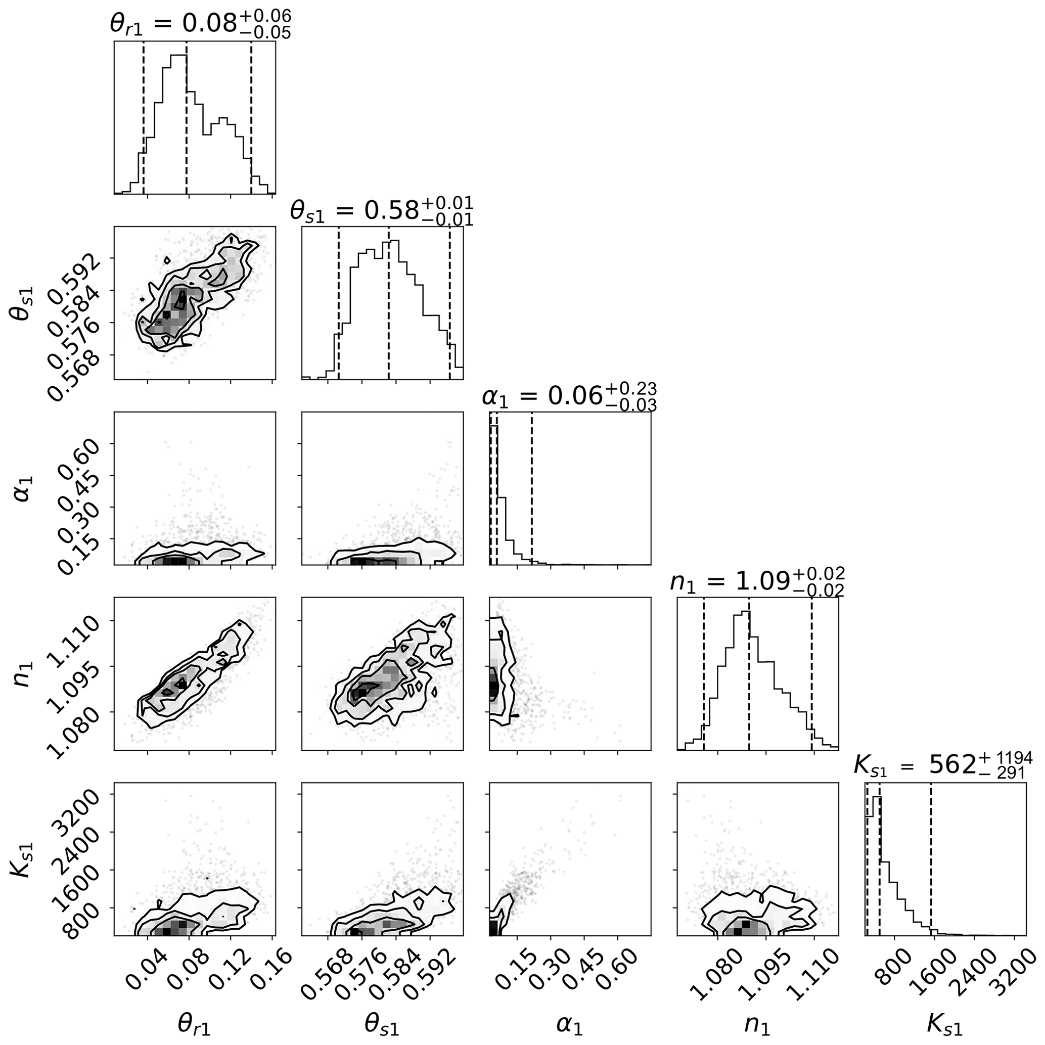
Figure A3Marginal posterior distributions (one-dimensional projection on top of each column and the joint distributions of each two parameters below) of estimated SHPs for the upper soil layer at Zettersfeld. Presented are the respective residual and saturated water content parameters θr and θs (cm3 cm−3), the VGM shape parameters α (cm−1) and n (–), and the saturated hydraulic conductivity parameter Ks (cm d−1).
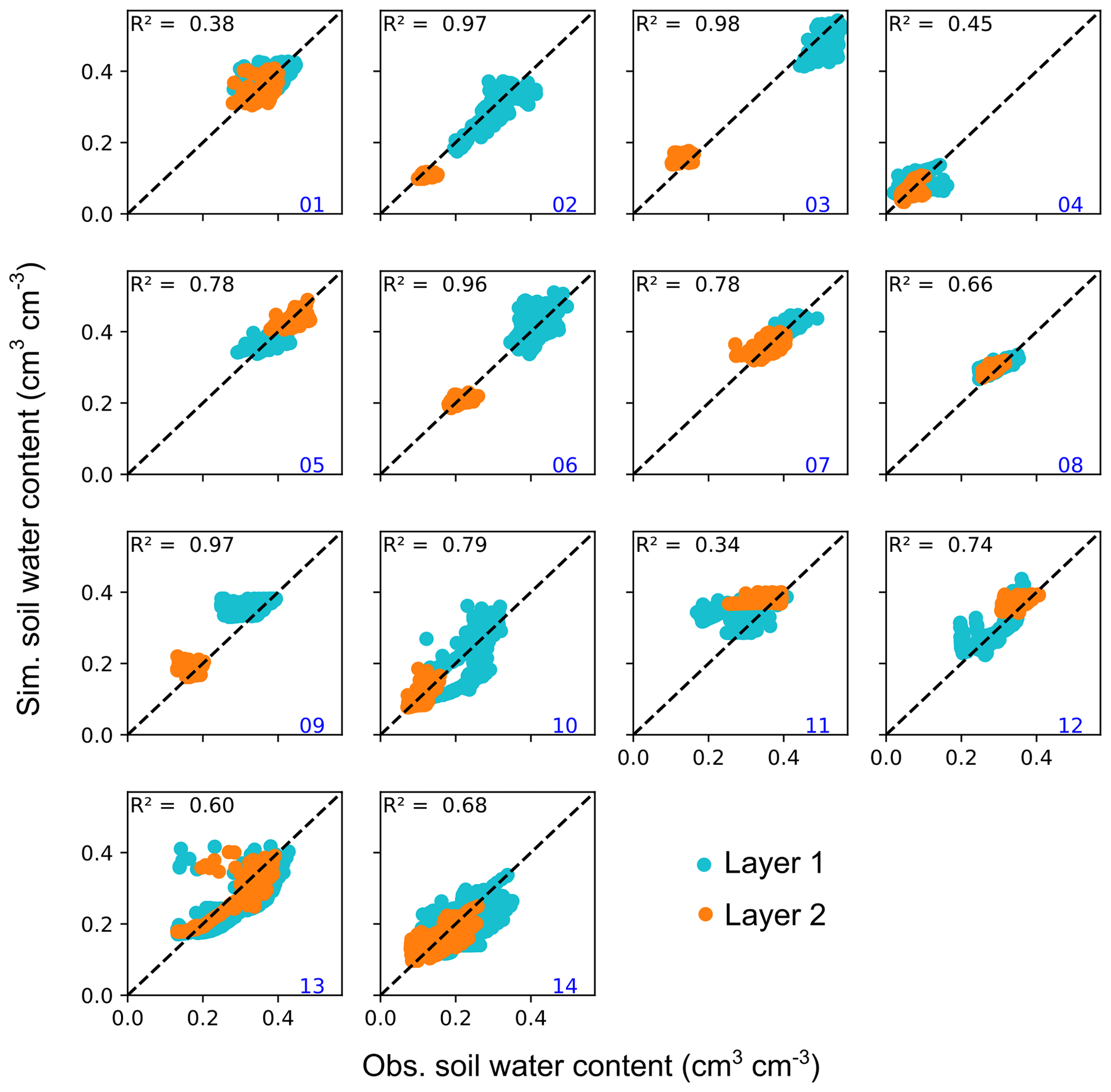
Figure A4Model validation showing the coefficient of determination (R2) and scatterplots of the simulated and observed soil water content from the upper (layer 1) and lower (layer 2) soil layers for the 14 sites: (01) Lauterach, (02) Leutasch, (03) Achenkirch, (04) Gschlössboden, (05) Sillianberger Alm, (06) Zettersfeld, (07) Elsbethen, (08) Gumpenstein, (09) Aichfeld-Murboden, (10) Kalsdorf, (11) Pettenbach, (12) Schalladorf, (13) Lobau, and (14) Frauenkirchen. The dashed diagonal black line is the 1:1 line. Validation periods are given in Table A2.
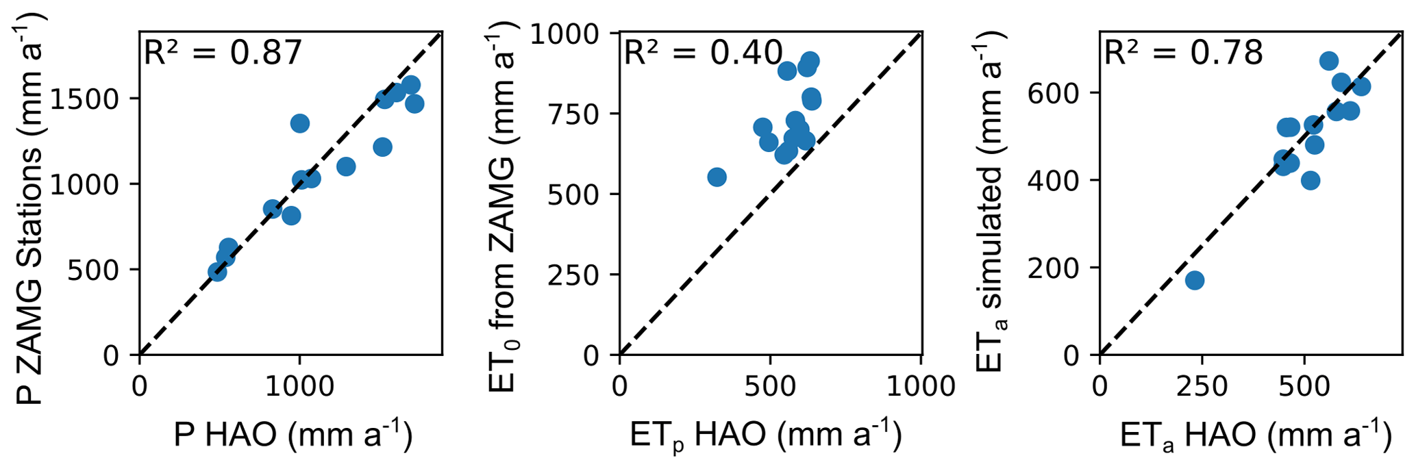
Figure A5Scatterplots comparing the long-term averages of precipitation (P) and potential and actual evapotranspiration (ETp and ETa, respectively) from the digital Hydrological Atlas of Austria (HAO) (BMLFUW, 2007) with the corresponding rates from simulations in this study. The dashed diagonal black is the 1:1 line. Potential evapotranspiration in the HAO was calculated by Dobesch (2007) using the FAO approach described by Doorenbos and Pruitt (1977), resulting in lower values than those of this study which were calculated for a grass reference according to Allen et al. (1998).
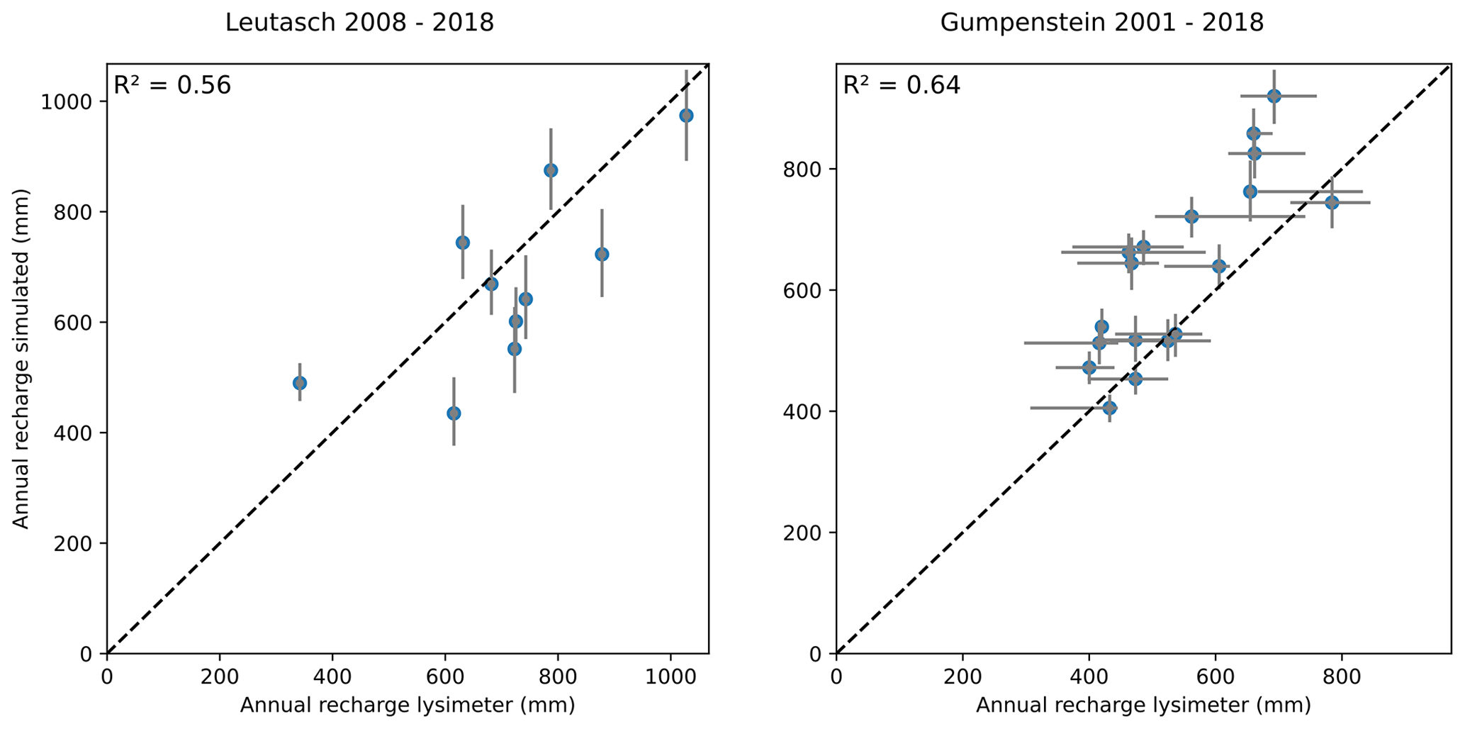
Figure A6Model validation using lysimeter data from Leutasch and Gumpenstein. Scatterplots and coefficients of determination (R2) are shown for simulated and observed annual seepage flow. Blue dots show median estimates and the gray error bars depict the 95 % credible interval from propagated parameter uncertainty. The dashed diagonal black line is the 1:1 line. Leutasch seepage measurements were obtained from a single lysimeter; for Gumpenstein, the 95 % uncertainty interval in the lysimeter measurements was calculated from a cluster of four lysimeters.
The software code of the HYDRUS-1D hydrological model is publicly available at https://www.pc-progress.com (PC-PROGRESS, 2023). The code for the MultiNest Bayesian inference tool is available at https://github.com/rjw57/MultiNest (Wareham, 2023). The reference entries for these third-party codes (given in the paper) are as follows:
-
HYDRUS – Šimůnek et al. (2016);
-
MultiNest – Feroz and Hobson (2008) and Feroz et al. (2009).
The raw data used in this study were generated in the framework of the soil water monitoring program conducted by the Austrian Federal Ministry of Agriculture, Forestry, Regions and Water Management (BML) and were shared with the authors of this study as part of the RechAUT project. Derived data supporting the findings of this study are available from the corresponding author (Marleen Schübl) upon request.
MS, GB, and CS designed the study. MS and GB performed the model simulations and contributed Python code for the analysis and data visualization. MS conducted the statistical analysis. GF curated and provided the original data. MS wrote the initial draft, and CS, GB, and GF reviewed and edited the manuscript. All authors revised the paper and agreed on its contents.
At least one of the (co-)authors is a member of the editorial board of Hydrology and Earth System Sciences. The peer-review process was guided by an independent editor, and the authors also have no other competing interests to declare.
Publisher's note: Copernicus Publications remains neutral with regard to jurisdictional claims in published maps and institutional affiliations.
This work was carried out in the framework of the RechAUT project and received support from the Austrian Academy of Sciences (ÖAW), Vienna, Austria. Meteorological data were provided by the Central Institution for Meteorology and Geodynamics (ZAMG), Vienna, Austria. Soil texture data for the Gschlössboden site were provided by the Hydrography and Hydrology Division of the Tyrolean Government. We would like to thank the reviewers, whose valuable input improved this paper.
This research has been supported by the Austrian Academy of Sciences (Österreichische Akademie der Wissenschaften, ÖAW) within the framework of the “Variabilität der Grundwasserneubildungsraten in Österreich (RechAUT)” project.
This paper was edited by Nunzio Romano and reviewed by Ty P. A. Ferre, Jasper Vrugt, and three anonymous referees.
Allen, R. G., Pereira, L. S., Raes, D., Smith, M., and Others: FAO Irrigation and drainage paper No. 56, Food and Agriculture Organization of the United Nations, Rome, http://www.climasouth.eu/sites/default/files/FAO 56.pdf (last access: 25 March 2023), 1998. a, b, c
Assefa, K. A. and Woodbury, A. D.: Transient, spatially varied groundwater recharge modeling, Water Resour. Res., 49, 4593–4606, https://doi.org/10.1002/wrcr.20332, 2013. a, b
Barkle, G., Wöhling, T., Stenger, R., Mertens, J., Moorhead, B., Wall, A., and Clague, J.: Automated Equilibrium Tension Lysimeters for Measuring Water Fluxes through a Layered, Volcanic Vadose Profile in New Zealand, Vadose Zone J., 10, 747–759, https://doi.org/10.2136/vzj2010.0091, 2011. a
Baroni, G., Facchi, A., Gandolfi, C., Ortuani, B., Horeschi, D., and Van Dam, J. C.: Uncertainty in the determination of soil hydraulic parameters and its influence on the performance of two hydrological models of different complexity, Hydrol. Earth Syst. Sci., 14, 251–270, https://doi.org/10.5194/hess-14-251-2010, 2010. a
Barron, O. V., Crosbie, R. S., Dawes, W. R., Charles, S. P., Pickett, T., and Donn, M. J.: Climatic controls on diffuse groundwater recharge across Australia, Hydrol. Earth Syst. Sci., 16, 4557–4570, https://doi.org/10.5194/hess-16-4557-2012, 2012. a, b
Berthelin, R., Rinderer, M., Andreo, B., Baker, A., Kilian, D., Leonhardt, G., Lotz, A., Lichtenwoehrer, K., Mudarra, M., Padilla, I. Y., Pantoja Agreda, F., Rosolem, R., Vale, A., and Hartmann, A.: A soil moisture monitoring network to characterize karstic recharge and evapotranspiration at five representative sites across the globe, Geosci. Instrum. Method. Data Syst., 9, 11–23, https://doi.org/10.5194/gi-9-11-2020, 2020. a
Beven, K.: A manifesto for the equifinality thesis, J. Hydrol., 320, 18–36, https://doi.org/10.1016/j.jhydrol.2005.07.007, 2006. a
Beven, K.: Facets of uncertainty: epistemic uncertainty, non-stationarity, likelihood, hypothesis testing, and communication, Hydrolog. Sci. J., 61, 1652–1665, 2016. a
BFW: Österreichische Bodenkartierung, https://bodenkarte.at/ (last access: 25 March 2023), 2016. a, b
BMLFUW: Hydrologischer Atlas Österreichs, ISBN 3-85437-250-7, 2007. a, b
Boumaiza, L., Chesnaux, R., Walter, J., and Stumpp, C.: Assessing groundwater recharge and transpiration in a humid northern region dominated by snowmelt using vadose-zone depth profiles, Hydrogeol. J., 28, 2315–2329, https://doi.org/10.1007/s10040-020-02204-z, 2020. a
Bresciani, E., Cranswick, R. H., Banks, E. W., Batlle-Aguilar, J., Cook, P. G., and Batelaan, O.: Using hydraulic head, chloride and electrical conductivity data to distinguish between mountain-front and mountain-block recharge to basin aquifers, Hydrol. Earth Syst. Sci., 22, 1629–1648, https://doi.org/10.5194/hess-22-1629-2018, 2018. a
Brunetti, G., Šimůnek, J., Bogena, H., Baatz, R., Huisman, J. A., Dahlke, H., and Vereecken, H.: On the Information Content of Cosmic‐Ray Neutron Data in the Inverse Estimation of Soil Hydraulic Properties, Vadose Zone J., 18, 1–24, https://doi.org/10.2136/vzj2018.06.0123, 2019. a, b
Brunetti, G., Papagrigoriou, I. A., and Stumpp, C.: Disentangling model complexity in green roof hydrological analysis: A Bayesian perspective, Water Res., 182, 115973, https://doi.org/10.1016/j.watres.2020.115973, 2020a. a, b
Brunetti, G., Šimůnek, J., Glöckler, D., and Stumpp, C.: Handling model complexity with parsimony: Numerical analysis of the nitrogen turnover in a controlled aquifer model setup, J. Hydrol., 584, 124681, https://doi.org/10.1016/j.jhydrol.2020.124681, 2020b. a, b, c
Brunetti, G., Schübl, M., Santner, K., and Stumpp, C.: Sensitivitätsanalyse zu Infiltrationsprozessen in Böden, Österreich. Wasser Abfallwirt., 74, 179–186, https://doi.org/10.1007/s00506-022-00839-8, 2022. a
Buchner, J.: A statistical test for Nested Sampling algorithms, Stat. Comput., 26, 383–392, https://doi.org/10.1007/s11222-014-9512-y, 2016. a
Burri, N. M., Weatherl, R., Moeck, C., and Schirmer, M.: A review of threats to groundwater quality in the anthropocene, Sci. Total Environ., 684, 136–154, https://doi.org/10.1016/j.scitotenv.2019.05.236, 2019. a
Cao, G., Scanlon, B. R., Han, D., and Zheng, C.: Impacts of thickening unsaturated zone on groundwater recharge in the North China Plain, J. Hydrol., 537, 260–270, https://doi.org/10.1016/j.jhydrol.2016.03.049, 2016. a
Chesnaux, R. and Stumpp, C.: Advantages and challenges of using soil water isotopes to assess groundwater recharge dominated by snowmelt at a field study located in Canada, Hydrolog. Sci. J., 63, 679–695, https://doi.org/10.1080/02626667.2018.1442577, 2018. a
Collenteur, R. A., Bakker, M., Klammler, G., and Birk, S.: Estimation of groundwater recharge from groundwater levels using nonlinear transfer function noise models and comparison to lysimeter data, Hydrol. Earth Syst. Sci., 25, 2931–2949, https://doi.org/10.5194/hess-25-2931-2021, 2021. a, b, c, d
Dettmann, U., Bechtold, M., Frahm, E., and Tiemeyer, B.: On the applicability of unimodal and bimodal van Genuchten-Mualem based models to peat and other organic soils under evaporation conditions, J. Hydrol., 515, 103–115, https://doi.org/10.1016/j.jhydrol.2014.04.047, 2014. a
Dobesch, H.: Hydrological Atlas of Austria – Mean annual potential evapotranspiration (3.2), Lebensministerium (BMLFUW), Vienna, 2007. a, b
Doble, R. C. and Crosbie, R. S.: Revue: Méthodes courantes et émergentes pour la modélisation de la recharge à l'échelle du bassin versant et de l'évapotranspiration d'eaux souterraines peu profondes, Hydrogeol. J., 25, 3–23, https://doi.org/10.1007/s10040-016-1470-3, 2017. a
Döll, P. and Fiedler, K.: Global-scale modeling of groundwater recharge, Hydrol. Earth Syst. Sci., 12, 863–885, https://doi.org/10.5194/hess-12-863-2008, 2008. a
Doorenbos, J. and Pruitt, W. O.: Crop evapotranspiration, FAO irrigation and drainage Paper 24, FAO, 1–145, https://www.posmet.ufv.br/wp-content/uploads/2015/08/LIVRO-385-Doorenbos-e-Pruitt-Guidelines-for-predicting-crop (last access: 25 March 2023), 1977. a
Durner, W., Jansen, U., and Iden, S. C.: Effective hydraulic properties of layered soils at the lysimeter scale determined by inverse modelling, Eur. J. Soil Sci., 59, 114–124, https://doi.org/10.1111/j.1365-2389.2007.00972.x, 2008. a
Dyck, M. and Kachanoski, R.: Spatial Scale-Dependence of Preferred Flow Domains during Infiltration in a Layered Field Soil, Vadose Zone J., 9, 385–396, https://doi.org/10.2136/vzj2009.0093, 2010. a
Elsheikh, A. H., Wheeler, M. F., and Hoteit, I.: Nested sampling algorithm for subsurface flow model selection, uncertainty quantification, and nonlinear calibration, Water Resour. Res., 49, 8383–8399, https://doi.org/10.1002/2012WR013406, 2013. a
Emerson, W. W.: Water retention, organic c and soil texture, Aust. J. Soil Res., 33, 241–251, https://doi.org/10.1071/SR9950241, 1995. a
Feddes, R. A., Kowalik, P. J., Zaradny, H., Taylor, S. A., Ashcroft, G. L., Vrugt, J. A., Diks, C. G., Gupta, H. V., Bouten, W., and Verstraten, J. M.: Physical edaphology. The physics of irrigated and nonirrigated soils, Monogr. PUDOC, Wageningen, 41, 1–17, https://doi.org/10.1029/2004WR003059, 1978. a
Feroz, F. and Hobson, M. P.: Multimodal nested sampling: An efficient and robust alternative to Markov Chain Monte Carlo methods for astronomical data analyses, Mon. Notice. Roy. Astron. Soc., 384, 449–463, https://doi.org/10.1111/j.1365-2966.2007.12353.x, 2008. a, b, c
Feroz, F., Hobson, M. P., and Bridges, M.: MultiNest: An efficient and robust Bayesian inference tool for cosmology and particle physics, Mon. Notice. Roy. Astron. Soc., 398, 1601–1614, https://doi.org/10.1111/j.1365-2966.2009.14548.x, 2009. a, b, c, d
Feroz, F., Hobson, M. P., Cameron, E., and Pettitt, A. N.: Importance Nested Sampling and the MultiNest Algorithm, Open J. Astrophys., 2, 1, https://doi.org/10.21105/astro.1306.2144, 2019. a
Finsterle, S.: Practical notes on local data-worth analysis, Water Resour. Res., 51, 9904–9924, https://doi.org/10.1002/2015WR017445, 2015. a
Fuentes, C., Haverkamp, R., and Parlange, J. Y.: Parameter constraints on closed-form soilwater relationships, J. Hydrol., 134, 117–142, https://doi.org/10.1016/0022-1694(92)90032-Q, 1992. a
Gao, H., Zhang, J., Liu, C., Man, J., Chen, C., Wu, L., and Zeng, L.: Efficient Bayesian Inverse Modeling of Water Infiltration in Layered Soils, Vadose Zone J., 18, 1–13, https://doi.org/10.2136/vzj2019.03.0029, 2019. a
Groh, J., Vanderborght, J., Pütz, T., and Vereecken, H.: How to Control the Lysimeter Bottom Boundary to Investigate the Effect of Climate Change on Soil Processes?, Vadose Zone J., 15, vzj2015.08.0113, https://doi.org/10.2136/vzj2015.08.0113, 2016. a
Groh, J., Stumpp, C., Lücke, A., Pütz, T., Vanderborght, J., and Vereecken, H.: Inverse Estimation of Soil Hydraulic and Transport Parameters of Layered Soils from Water Stable Isotope and Lysimeter Data, Vadose Zone J., 17, 170168, https://doi.org/10.2136/vzj2017.09.0168, 2018. a, b
Gupta, A., Govindaraju, R. S., Morbidelli, R., and Corradini, C.: The Role of Prior Probabilities on Parameter Estimation in Hydrological Models, Water Resour. Res., 58, e2021WR031291, https://doi.org/10.1029/2021WR031291, 2022. a
Hartmann, A., Goldscheider, N., Wagener, T., Lange, J., and Weiler, M.: Karst water resources in a changing world: Review of hydrological modeling approaches, Rev. Geophys., 52, 218–242, https://doi.org/10.1002/2013RG000443, 2014. a
Hartmann, A., Gleeson, T., Wada, Y., and Wagener, T.: Enhanced groundwater recharge rates and altered recharge sensitivity to climate variability through subsurface heterogeneity, P. Natl. Acad. Sci. USA, 114, 2842–2847, https://doi.org/10.1073/pnas.1614941114, 2017. a
Healy, R. W. and Cook, P. G.: Using groundwater levels to estimate recharge, Hydrogeol. J., 10, 91–109, https://doi.org/10.1007/s10040-001-0178-0, 2002. a
Heilig, A., Steenhuis, T. S., Walter, M. T., and Herbert, S. J.: Funneled flow mechanisms in layered soil: Field investigations, J. Hydrol., 279, 210–223, https://doi.org/10.1016/S0022-1694(03)00179-3, 2003. a
Heppner, C. S., Nimmo, J. R., Folmar, G. J., Gburek, W. J., and Risser, D. W.: Multiple-methods investigation of recharge at a humid-region fractured rock site, Pennsylvania, USA, Hydrogeol. J., 15, 915–927, https://doi.org/10.1007/s10040-006-0149-6, 2007. a, b
Jarvis, N. J.: The MACRO model (Version 3.1) – Technical Description and Sample Simulations, p. 51, https://agris.fao.org/agris-search/search.do?recordID=SE19950122727 (last access: 25 March 2023), 1994. a
Kaminsky, E., Plan, L., Wagner, T., Funk, B., and Oberender, P.: Flow dynamics in a vadose shaft – a case study from the hochschwab karst massif (Northern calcareous alps, austria), Int. J. Speleol., 50, 157–172, https://doi.org/10.5038/1827-806X.50.2.2375, 2021. a
Keese, K. E., Scanlon, B. R., and Reedy, R. C.: Assessing controls on diffuse groundwater recharge using unsaturated flow modeling, Water Resour. Res., 41, 1–12, https://doi.org/10.1029/2004WR003841, 2005. a
Kling, H., Nachtnebel, H. P., and Fürst, J.: Hydrological Atlas of Austria – Mean annual areal actual evapotranspiration (3.3), Lebensministerium (BMLFUW), Vienna, 2007a. a, b, c, d
Kling, H., Nachtnebel, H. P., and Fürst, J.: Hydrological Atlas of Austria – Mean annual areal precipitation (2.3), Lebensministerium (BMLFUW), Vienna, 2007b. a, b, c
Koeniger, P., Gaj, M., Beyer, M., and Himmelsbach, T.: Review on soil water isotope-based groundwater recharge estimations, Hydrol. Process., 30, 2817–2834, https://doi.org/10.1002/hyp.10775, 2016. a
Lambot, S., Javaux, M., Hupet, F., and Vanclooster, M.: A global multilevel coordinate search procedure for estimating the unsaturated soil hydraulic properties, Water Resour. Res., 38, 6-1–6-15, https://doi.org/10.1029/2001wr001224, 2002. a
Land OÖ: Forschungsprojekt Lysimeter, Technischer Endbericht 2013, Tech. rep., Amt der Oöo. Landesregierung, Abteilung Grund- und Trinkwasserwirtschaft, Linz, https://www.land-oberoesterreich.gv.at/Mediendateien/Formulare/Dokumente UWD Abt_WW/2013_LysimeterO%C3%96_Jahresbericht13.pdf (last access: 25 March 2023), 2013. a
Land OÖ: Forschungsprojekt Lysimeter, Technischer Endbericht 2014, Tech. rep., Amt der Oö. Landesregierung, Abteilung Grund- und Trinkwasserwirtschaft, Linz, https://www.land-oberoesterreich.gv.at/Mediendateien/Formulare/Dokumente UWD Abt_WW/2014_LysimeterO%C3%96_Jahresbericht14.pdf (last access: 25 March 2023), 2014. a
Lu, J., Zhang, Q., Werner, A. D., Li, Y., Jiang, S., and Tan, Z.: Root-induced changes of soil hydraulic properties – A review, J. Hydrol., 589, 125203, https://doi.org/10.1016/j.jhydrol.2020.125203, 2020. a
Minasny, B. and Field, D. J.: Estimating soil hydraulic properties and their uncertainty: The use of stochastic simulation in the inverse modelling of the evaporation method, Geoderma, 126, 277–290, https://doi.org/10.1016/j.geoderma.2004.09.015, 2005. a
Mishra, S., Parker, J. C., and Singhal, N.: Estimation of soil hydraulic properties and their uncertainty from particle size distribution data, J. Hydrol., 108, 1–18, https://doi.org/10.1016/0022-1694(89)90275-8, 1989. a
Moeck, C., von Freyberg, J., and Schirmer, M.: Groundwater recharge predictions in contrasted climate: The effect of model complexity and calibration period on recharge rates, Environ. Model. Softw., 103, 74–89, https://doi.org/10.1016/j.envsoft.2018.02.005, 2018. a, b
Moeck, C., Grech-Cumbo, N., Podgorski, J., Bretzler, A., Gurdak, J. J., Berg, M., and Schirmer, M.: A global-scale dataset of direct natural groundwater recharge rates: A review of variables, processes and relationships, Sci. Total Environ., 717, 137042, https://doi.org/10.1016/j.scitotenv.2020.137042, 2020. a, b, c, d, e, f, g, h, i, j
Mualem, Y.: A new model for predicting the hydraulic conductivity of unsaturated porous media, Water Resour. Res., 12, 513–522, https://doi.org/10.1029/WR012i003p00513, 1976. a
Mukherjee, P., Parkinson, D., and Liddle, A. R.: A Nested Sampling Algorithm for Cosmological Model Selection, Astrophys. J., 638, L51–L54, https://doi.org/10.1086/501068, 2006. a, b
Neukum, C. and Azzam, R.: Impact of climate change on groundwater recharge in a small catchment in the Black Forest, Germany, Hydrogeol. J., 20, 547–560, https://doi.org/10.1007/s10040-011-0827-x, 2012. a
Neukum, C., Hötzl, H., and Himmelsbach, T.: Validation of vulnerability mapping methods by field investigations and numerical modelling, Hydrogeol. J., 16, 641–658, https://doi.org/10.1007/s10040-007-0249-y, 2008. a
Nolan, B. T., Healy, R. W., Taber, P. E., Perkins, K., Hitt, K. J., and Wolock, D. M.: Factors influencing ground-water recharge in the eastern United States, J. Hydrol., 332, 187–205, https://doi.org/10.1016/j.jhydrol.2006.06.029, 2007. a, b
Nolz, R., Cepuder, P., and Eitzinger, J.: Comparison of lysimeter based and calculated ASCE reference evapotranspiration in a subhumid climate, Theor. Appl. Climatol., 124, 315–324, https://doi.org/10.1007/s00704-015-1417-y, 2016. a
ÖNORM L 1050: ÖNORM L 1050, 2004: Boden als Pflanzenstandort – Begriffe und Untersuchungsverfahren, https://www.bdb.at/Service/NormenDetail?id=560339 (last access: 25 March 2023), 2016. a, b
PC-PROGRESS: HYDRUS-1D, https://www.pc-progress.com, last access: 1 April 2023. a
Pedregosa, F., Varoquaux, G., Gramfort, A., Michel, V., Thirion, B., Grisel, O., Blondel, M., Prettenhofer, P., Weiss, R., Dubourg, V., Vanderplas, J., Passos, A., Cournapeau, D., Brucher, M., Perrot, M., and Duchesnay, E.: Scikit-learn: Machine Learning in Python, J. Mach. Learn. Res., 12, 2825–2830, 2011. a, b
Pütz, T., Fank, J., and Flury, M.: Lysimeters in Vadose Zone Research, Vadose Zone J., 17, 180035, https://doi.org/10.2136/vzj2018.02.0035, 2018. a
QGIS Development Team: QGIS Geographic Information System, QGIS Association, https://www.qgis.org (last access: 25 March 2023), 2022. a
Rimon, Y., Dahan, O., Nativ, R., and Geyer, S.: Water percolation through the deep vadose zone and groundwater recharge: Preliminary results based on a new vadose zone monitoring system, Water Resour. Res., 43, W05402, https://doi.org/10.1029/2006WR004855, 2007. a
Ritter, A., Hupet, F., Muñoz-Carpena, R., Lambot, S., and Vanclooster, M.: Using inverse methods for estimating soil hydraulic properties from field data as an alternative to direct methods, Agr. Water Manage., 59, 77–96, https://doi.org/10.1016/S0378-3774(02)00160-9, 2003. a
Romano, N. and Santini, A.: Determining soil hydraulic functions from evaporation experiments by a parameter estimation approach: Experimental verifications and numerical studies, Water Resour. Res., 35, 3343–3359, https://doi.org/10.1029/1999WR900155, 1999. a
Scanlon, B. R., Healy, R. W., and Cook, P. G.: Choosing appropriate techniques for quantifying groundwater recharge, Hydrogeol. J., 10, 18–39, https://doi.org/10.1007/s10040-001-0176-2, 2002. a, b
Schaap, M. G. and Leij, F. J.: Using neural networks to predict soil water retention and soil hydraulic conductivity, Soil Till. Res., 47, 37–42, https://doi.org/10.1016/S0167-1987(98)00070-1, 1998. a
Scharnagl, B., Vrugt, J. A., Vereecken, H., and Herbst, M.: Inverse modelling of in situ soil water dynamics: Investigating the effect of different prior distributions of the soil hydraulic parameters, Hydrol. Earth Syst. Sci., 15, 3043–3059, https://doi.org/10.5194/hess-15-3043-2011, 2011. a, b, c
Schelle, H., Iden, S. C., Fank, J., and Durner, W.: Inverse Estimation of Soil Hydraulic and Root Distribution Parameters from Lysimeter Data, Vadose Zone J., 11, vzj2011.0169, https://doi.org/10.2136/vzj2011.0169, 2012. a, b
Schjønning, P., Munkholm, L. J., Moldrup, P., and Jacobsen, O. H.: Modelling soil pore characteristics from measurements of air exchange: The long-term effects of fertilization and crop rotation, Eur. J. Soil Sci., 53, 331–339, https://doi.org/10.1046/j.1365-2389.2002.00438.x, 2002. a
Schneider, S., Jacques, D., and Mallants, D.: Inverse modelling with a genetic algorithm to derive hydraulic properties of a multi-layered forest soil, Soil Res., 51, 372–389, https://doi.org/10.1071/SR13144, 2013. a
Schübl, M., Stumpp, C., and Brunetti, G.: A Bayesian perspective on the information content of soil water measurements for the hydrological characterization of the vadose zone, J. Hydrol., 613, 128429, https://doi.org/10.1016/j.jhydrol.2022.128429, 2022. a, b, c, d, e
Seneviratne, S. I., Lehner, I., Gurtz, J., Teuling, A. J., Lang, H., Moser, U., Grebner, D., Menzel, L., Schroff, K., Vitvar, T., and Zappa, M.: Swiss prealpine Rietholzbach research catchment and lysimeter: 32 year time series and 2003 drought event, Water Resour. Res., 48, W06526, https://doi.org/10.1029/2011WR011749, 2012. a
Šimůnek, J.: Estimating groundwater recharge using HYDRUS-1D, Geological Institute, Bulgarian Academy of Sciences, 29, 25–36, https://www.pc-progress.com/Documents/Jirka/Simunek_EnginGeolHydrogeol_2016.pdf (last access: 25 March 2023), 2015. a
Šimůnek, J., Jarvis, N. J., Van Genuchten, M. T., and Gärdenäs, A.: Review and comparison of models for describing non-equilibrium and preferential flow and transport in the vadose zone, J. Hydrol., 272, 14–35, https://doi.org/10.1016/S0022-1694(02)00252-4, 2003. a
Šimůnek, J., van Genuchten, M. T., and Šejna, M.: Recent Developments and Applications of the HYDRUS Computer Software Packages, Vadose Zone J., 15, vzj2016.04.0033, https://doi.org/10.2136/vzj2016.04.0033, 2016. a, b, c
Skilling, J.: Nested sampling for general Bayesian computation, Bayes. Anal., 1, 833–860, https://doi.org/10.1214/06-BA127, 2006. a, b
Stumpp, C., Maloszewski, P., Stichler, W., and Fank, J.: Environmental isotope (δ18O) and hydrological data to assess water flow in unsaturated soils planted with different crops: Case study lysimeter station “Wagna” (Austria), J. Hydrol., 369, 198–208, https://doi.org/10.1016/j.jhydrol.2009.02.047, 2009. a
Stumpp, C., Stichler, W., Kandolf, M., and Šimůnek, J.: Effects of Land Cover and Fertilization Method on Water Flow and Solute Transport in Five Lysimeters: A Long-Term Study Using Stable Water Isotopes, Vadose Zone J., 11, 1, https://doi.org/10.2136/vzj2011.0075, 2012. a, b
Taylor, R. G., Scanlon, B., Döll, P., Rodell, M., Van Beek, R., Wada, Y., Longuevergne, L., Leblanc, M., Famiglietti, J. S., Edmunds, M., Konikow, L., Green, T. R., Chen, J., Taniguchi, M., Bierkens, M. F., Macdonald, A., Fan, Y., Maxwell, R. M., Yechieli, Y., Gurdak, J. J., Allen, D. M., Shamsudduha, M., Hiscock, K., Yeh, P. J., Holman, I., and Treidel, H.: Ground water and climate change, Nat. Clim. Change, 3, 322–329, https://doi.org/10.1038/nclimate1744, 2013. a, b
Taylor, S. A. and Ashcroft, G. L.: Physical edaphology. The physics of irrigated and nonirrigated soils, https://www.cabdirect.org/cabdirect/abstract/19731901994 (last access: 25 March 2023), 1972. a
Tóth, G., Rman, N., Ágnes, R. S., Kerékgyártó, T., Szocs, T., Lapanje, A., Černák, R., Remsík, A., Schubert, G., and Nádor, A.: Transboundary fresh and thermal groundwater flows in the west part of the Pannonian Basin, Renew. Sustain. Energ. Rev., 57, 439–454, https://doi.org/10.1016/j.rser.2015.12.021, 2016. a
Van Genuchten, M. T.: A closed-form equation for predicting the hydraulic conductivity of unsaturated soils, Soil Sci. Soc. Am. J., 44, 892–898, 1980. a
Vereecken, H., Huisman, J. A., Bogena, H., Vanderborght, J., Vrugt, J. A., and Hopmans, J. W.: On the value of soil moisture measurements in vadose zone hydrology: A review, Water Resour. Res., 46, W00D06, https://doi.org/10.1029/2008WR006829, 2008. a, b
Vereecken, H., Schnepf, A., Hopmans, J., Javaux, M., Or, D., Roose, T., Vanderborght, J., Young, M., Amelung, W., Aitkenhead, M., Allison, S., Assouline, S., Baveye, P., Berli, M., Brüggemann, N., Finke, P., Flury, M., Gaiser, T., Govers, G., Ghezzehei, T., Hallett, P., Hendricks Franssen, H., Heppell, J., Horn, R., Huisman, J., Jacques, D., Jonard, F., Kollet, S., Lafolie, F., Lamorski, K., Leitner, D., McBratney, A., Minasny, B., Montzka, C., Nowak, W., Pachepsky, Y., Padarian, J., Romano, N., Roth, K., Rothfuss, Y., Rowe, E., Schwen, A., Šimůnek, J., Tiktak, A., Van Dam, J., van der Zee, S., Vogel, H., Vrugt, J., Wöhling, T., and Young, I.: Modeling Soil Processes: Review, Key Challenges, and New Perspectives, Vadose Zone J., 15, vzj2015.09.0131, https://doi.org/10.2136/vzj2015.09.0131, 2016. a, b
Vogel, W.: Österreich – Vorreiter im Grundwasserschutz, Ländlicher Raum, p. 12, https://info.bml.gv.at/dam/jcr:e19e56b5-fc51-4b9e-b5f0-966d8f220bbf/41_Wilhelm ogel - %C3%96sterreich - Vorreiter im Grundwasserschutz.pdf (last access: 25 March 2023), 2001. a
von Freyberg, J., Moeck, C., and Schirmer, M.: Estimation of groundwater recharge and drought severity with varying model complexity, J. Hydrol., 527, 844–857, https://doi.org/10.1016/j.jhydrol.2015.05.025, 2015. a, b
Vrugt, J. A. and Sadegh, M.: Toward diagnostic model calibration and evaluation: Approximate Bayesian computation, Water Resour. Res., 49, 4335–4345, https://doi.org/10.1002/wrcr.20354, 2013. a
Vrugt, J. A., Bouten, W., Gupta, H. V., and Hopmans, J. W.: Toward improved identifiability of soil hydraulic parameters: On the selection of a suitable parametric model, Vadose Zone J., 2, 98–113, 2003. a
Vrugt, J. A., ter Braak, C. J. F., Clark, M. P., Hyman, J. M., and Robinson, B. A.: Treatment of input uncertainty in hydrologic modeling: Doing hydrology backward with Markov chain Monte Carlo simulation, Water Resour. Res., 44, W00B09, https://doi.org/10.1029/2007wr006720, 2008. a
Vrugt, J. A., de Oliveira, D. Y., Schoups, G., and Diks, C. G.: On the use of distribution-adaptive likelihood functions: Generalized and universal likelihood functions, scoring rules and multi-criteria ranking, J. Hydrol., 615, 128542, https://doi.org/10.1016/j.jhydrol.2022.128542, 2022. a
Wareham, R.: rjw57/MultiNest, GitHub [code], https://github.com/rjw57/MultiNest, last access: 1 April 2023. a
Wang, T., Istanbulluoglu, E., Lenters, J., and Scott, D.: On the role of groundwater and soil texture in the regional water balance: An investigation of the Nebraska Sand Hills, USA, Water Resour. Res., 45, W10413, https://doi.org/10.1029/2009WR007733, 2009. a
Wesseling, J., Elbers, J., Kabat, P., and Van den Broek, B.: SWATRE: Instructions for input, Internal Note, Winand Staring Centre, Wageningen, the Netherlands, 1991. a
Whalley, W. R., Riseley, B., Leeds-Harrison, P. B., Bird, N. R., Leech, P. K., and Adderley, W. P.: Structural differences between bulk and rhizosphere soil, Eur. J. Soil Sc., 56, 353–360, https://doi.org/10.1111/j.1365-2389.2004.00670.x, 2005. a
Wohling, D. L., Leaney, F. W., and Crosbie, R. S.: Deep drainage estimates using multiple linear regression with percent clay content and rainfall, Hydrol. Earth Syst. Sci., 16, 563–572, https://doi.org/10.5194/hess-16-563-2012, 2012. a
Wöhling, T., Vrugt, J. A., and Barkle, G. F.: Comparison of Three Multiobjective Optimization Algorithms for Inverse Modeling of Vadose Zone Hydraulic Properties, Soil Sci. Soc. Am. J., 72, 305–319, https://doi.org/10.2136/sssaj2007.0176, 2008. a, b
Wöhling, T., Schöniger, A., Gayler, S., and Nowak, W.: Bayesian model averaging to explore the worth of data for soil-plant model selection and prediction, Water Resour. Res., 51, 2825–2846, https://doi.org/10.1002/2014WR016292, 2015. a
Xie, Y., Cook, P. G., Simmons, C. T., Partington, D., Crosbie, R., and Batelaan, O.: Uncertainty of groundwater recharge estimated from a water and energy balance model, J. Hydrol., 561, 1081–1093, https://doi.org/10.1016/j.jhydrol.2017.08.010, 2018. a
Zhao, Y., Peth, S., Horn, R., Šimůnek, J., and Kodešová, R.: Modeling of coupled water and heat fluxes in both unfrozen and frozen soils, in: Proc. of HYDRUS Workshop, Czech University of Life Sciences, Prague, Czech, 55–60, http://pc-progress.com/Documents/Workshop_2008_Prague/Proceedings - Prague's HYDRUS Worskshop.pdf#page=59 (last access: 25 March 2023), 2008. a