the Creative Commons Attribution 4.0 License.
the Creative Commons Attribution 4.0 License.
 | 31 Mar 2023
Hyper-resolution PCR-GLOBWB: opportunities and challenges from refining model spatial resolution to 1 km over the European continent
Edwin H. Sutanudjaja
Niko Wanders
Rens L. P. H. van Beek
Marc F. P. Bierkens
The quest for hydrological hyper-resolution modelling has been on-going for more than a decade. While global hydrological models (GHMs) have seen a reduction in grid size, they have thus far never been consistently applied at a hyper-resolution ( km) at the large scale. Here, we present the first application of the GHM PCR-GLOBWB at 1 km over Europe. We thoroughly evaluated simulated discharge, evaporation, soil moisture, and terrestrial water storage anomalies against long-term observations and subsequently compared results with the established 10 and 50 km resolutions of PCR-GLOBWB. Subsequently, we could assess the added value of this first hyper-resolution version of PCR-GLOBWB and assess the scale dependencies of model and forcing resolution. Eventually, these insights can help us in understanding the current challenges and opportunities from hyper-resolution models and in formulating the model and data requirements for future improvements.
We found that, for most variables, epistemic uncertainty is still large, and issues with scale commensurability exist with respect to the long-term yet coarse observations used. Merely for simulated discharge, we can confidently state that model output at hyper-resolution improves over coarser resolutions due to better representation of the river network at 1 km. However, currently available observations are not yet widely available at hyper-resolution or lack a sufficiently long time series, which makes it difficult to assess the performance of the model for other variables at hyper-resolution. Here, additional model validation efforts are needed. On the model side, hyper-resolution applications require careful revisiting of model parameterization and possibly the implementation of more physical processes to be able to resemble the dynamics and spatial heterogeneity at 1 km.
With this first application of PCR-GLOBWB at 1 km, we contribute to meeting the grand challenge of hyper-resolution modelling. Even though the model was only assessed at the continental scale, valuable insights could be gained which have global validity. As such, it should be seen as a modest milestone on a longer journey towards locally relevant model output. This, however, requires a community effort from domain experts, model developers, research software engineers, and data providers.
- Article
(7789 KB) - Full-text XML
- BibTeX
- EndNote


Climate change is projected to impact the patterns and intensity of precipitation and temperature worldwide, resulting in the increased occurrence of hydrological extremes and, in turn, rising hazard probability and risk globally (Dottori et al., 2018; Hirabayashi et al., 2013; Winsemius et al., 2016; Ward et al., 2020b; van der Wiel et al., 2019). To explore large-scale climate adaption options and mitigation measures, in addition to the efficacy of risk management plans, output from global hydrological models (GHMs) is increasingly employed as a basis for discussion and policy-making. Examples are the Aqueduct Global Flood Analyzer (2021; Ward et al., 2020a), the Aqueduct Water Risk Atlas (Hofste et al., 2019), the World Wildlife Fund for Nature (WWF) Water Risk Filter (WWF, 2022), and Water2Invest (Straatsma et al., 2020; water2invest web service, 2021).
One of the main advantages of GHMs is that their outputs are readily available and provide spatially and temporally consistent estimates of hazard probability and risks (Bierkens, 2015). However, global climate change impacts are often evaluated at the level of river basins or at country scale. Therefore, it is critical that the use of GHMs, which typically employ a relatively coarse spatial resolution (≥5 arcmin; equivalent to around 100 km2 at the Equator), is fit for purpose and that the current GHMs are used as intended (Ward et al., 2015). Nevertheless, the actual impact of hydrologic hazards happens at the local level and may vary greatly within countries, which pushes the boundaries of applicability of the current generation of GHMs. To capture these important spatial variations and to eventually make GHMs “locally relevant” (Bierkens et al., 2015) and usable by local water managers (Beven and Cloke, 2012), it is hence the current understanding that models need to move towards “hyper-resolution” (Wood et al., 2011; Bierkens et al., 2015), that is, to a spatial resolution below 1 km2 (30 arcsec). With hydrologic hazards already having increased and being projected to increase further (see, e.g., Winsemius et al., 2016; Alfieri et al., 2017; Samaniego et al., 2018; van der Wiel et al., 2019; also see the work of the World Weather Attribution initiative in Kew et al., 2021, and Philip et al., 2019), it is paramount to better understand their impact not only for entire economies but also more granularly on the sub-national to community level. Once an actionable local model output becomes available, large-scale and target-oriented adaptation and mitigation measures can be devised.
Global models have their own raison d'etre, as discussed in Ward et al. (2015), for instance, analyses over data-sparse areas or continuous transboundary simulations, thereby complementing bespoke local and country-scale models which may already be able to run at hyper-resolution. Moving towards hyper-resolution may potentially improve these analyses and, as a result, their meaningfulness and applicability. However, due to issues with, inter alia, model parameterization and computational demand, running GHMs at a meaningful and actionable spatial resolution over large extents was considered to be a “grand challenge” (Bierkens et al., 2015; Wood et al., 2011).
With computational power increasing and input datasets becoming available at ever finer spatial resolutions, the spatial resolution of current GHMs has increased in past years too. Currently, most GHMs can be run globally at a resolution of 5 to 6 arcmin, according to Bierkens et al. (2015). However, a grid cell at a resolution of 5 arcmin still translates to roughly 102 km2 at the Equator. Recently, various modelling attempts were made to further increase spatial resolution or to pave the way towards hyper-resolution. For example, the HydroBlocks model (Chaney et al., 2016) was coupled with remotely sensed data to obtain soil moisture estimates at 30 m spatial resolution over the continental United States of America (CONUS; Vergopolan et al., 2020, 2021). While HydroBlocks brings the simulations to an effective 30 m resolution, it still takes advantages of grouping regions based on hydrological similarity to reduce computational demands. O'Neill et al. (2021) applied and evaluated the hydrological model ParFlow (Maxwell et al., 2015) configured over the CONUS at 1 km spatial resolution, covering the years 2003 until 2006, constituting first-of-its-kind studies covering such an extensive area at true hyper-resolution. Aerts et al. (2022) assessed changes in model accuracy of the hydrological model wflow_sbm (Schellekens et al., 2020) at multiple resolutions below 1 km2 for the CAMELS dataset (Catchment Attributes and MEteorology for Large-sample Studies; Newman et al., 2015; Addor et al., 2017), again solely covering the CONUS. While the spatial resolution applied is hyper-resolution, the lack of either spatially continuous simulations over large extents or short simulation periods makes it challenging to define a substantial benchmark that is representative to the realm of GHMs. Other studies already proposed scalable routing networks (Thober et al., 2019) and measure how to seamlessly model across scales (Samaniego et al., 2010, 2017), which are essential when moving towards hyper-resolution.
On a more general note, the call for hyper-resolution is strongly driven by an expected increase in model accuracy and consequently applicability. One hypothesis thus is that particularly locations with a small upstream area will profit as more interactions will be simulated there and that the representation of the storage and response times in these regions is improved. The question of whether this is really the case depends also on the ability to populate the many fine-resolution cells with accurate parameters (Wood et al., 2011; Beven and Cloke, 2012). It is believed that this is not possible without additional locally specific information, and as such, Beven et al. (2015) concluded that hyper-resolution modelling will not achieve the necessary accuracy. Thus, we first need to establish an understanding of to what extent the accuracy of GHMs is improved when only their resolution is increased while still employing globally available datasets currently used for parameterizing GHMs. Even though models at different resolutions should ideally use bespoke parameterization and input data when applied at these three resolutions, we kept both as unaltered as possible to be able to better separate the impact of spatial resolution.
A second avenue towards improved model accuracy is the use of more accurate meteorological forcing. In studies using GHMs, it is shown that particularly the quality and spatial resolution of meteorological variables, notably precipitation, can have a pronounced impact on model accuracy (Beck et al., 2020; Towner et al., 2019; Biemans et al., 2009). Hence, a second question is raised as to whether it is necessary to go all the way to model hyper-resolution or if using forced hyper-resolution with the current GHMs already suffices. This would reduce the need for updated model parameterization and design, in addition to greatly shortening run times and reducing model data storage requirements. A locally relevant spatial resolution could then be achieved using post-processing tools, for instance.
The main objective of this paper is therefore to increase our understanding of the scale dependencies of both the model and the meteorological input and formulate ways forward towards meeting the above-named grand challenge. To that end, we developed a 30 arcsec (∼1 km) version of the existing 10 km PCR-GLOBWB model (Sutanudjaja et al., 2018) for the entire European continent and applied it over the period 1981 until 2019. As such, it constitutes a first-of-its-kind effort to set up, run, and evaluate a GHM at hyper-resolution over multiple decades. We acknowledge that this constitutes only a continental-scale application of a global model, but the study set up and choice of datasets has been made such that both methods and findings can potentially be transferred to the global scale. The main reason for focusing on Europe only is that the data richness there improves our ability to better create and evaluate models. The model was used to test how a stepwise increase in spatial resolution (30 arcmin/∼50 km, 5 arcmin/∼10 km, and 30 arcsec/∼1 km) impacts model accuracy. To test the impact of the forcing resolution, the model simulations at the different spatial resolutions were forced with ERA5-Land data (Muñoz-Sabater et al., 2021) at the same spatial resolutions or coarser. Finally, we combine both experiments to disentangle the relative importance of the model and forcing resolution. Except for the precipitation forcing, all simulations make use of the same input and parameter sets and are downscaled or upscaled only if necessary. In our analysis, we focus not merely on simulated discharge, as done by Aerts et al. (2022), for instance, but also on terrestrial water storage anomalies, evaporation, and soil moisture to provide a more holistic picture of model performance than what is typically the norm (see O'Neill et al., 2021). Such a very first thorough analysis of a hyper-resolution GHM is in the first place not intended to claim that hyper-resolution should be the new normal for GHMs but rather to gather opportunities and challenges of the scale dependencies of refining the spatial resolution of the model and its forcing. These insights may help in identifying the most effective model development pathways and advancing current efforts to produce spatially consistent and locally relevant estimates at (sub-)kilometre scale.
2.1 Study area and input data
In addition to the already-existing global schematizations of PCR-GLOBWB at 30 arcmin (roughly 50 km cell length at the Equator) and 5 arcmin (roughly 10 km cell length at the Equator), respectively, we developed a novel 30 arcsec (roughly 1 km cell length at the Equator) schematization.
The study period for which each run was executed is 1981 until 2019 at a daily time step. However, to reduce storage requirements, and due to the time step of most observations, our evaluations focused on the monthly time step, except for discharge analysis, where both the daily and monthly time step were used.
Each of the model resolutions (note that the term “resolution” refers to the spatial resolution throughout this paper, unless specifically stated otherwise) was forced with precipitation at the model resolution or coarser, yielding in total six combinations of model and forcing spatial resolutions (see Table 1).
Table 1Overview of model and forcing in addition to the run names used.
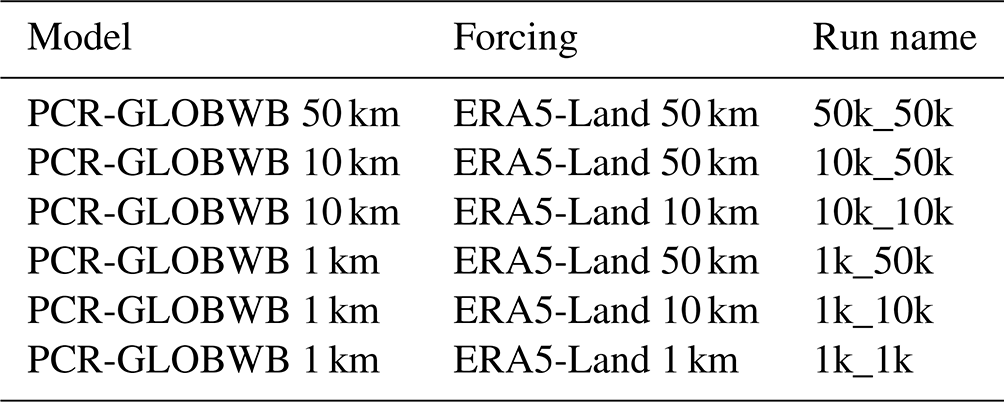
For all three spatial resolutions, identical model input data and parameter sets are used to guarantee comparability across set-ups. The default resolution is 1 km, meaning that all model development including runoff, soil, and groundwater processes was geared towards this resolution, and all other resolutions are derivatives. A detailed overview of the datasets used for model parameterization and forcing input can be found in Appendix A1, including the scaling techniques used to derive them at various resolutions (i.e. 1, 30, and 50 km). It should be mentioned here that resampling the default 1 km data to a coarser resolution affects model schematization (Samaniego et al., 2017), although the greatest care was taken to minimize this effect. Hence, the impact of using different model resolutions is not assessed in isolation but rather in its bigger context of how the model schematization would appear for a given model resolution. Each run includes water demand and use for irrigation, industry, livestock, and household, as well as accounting for reservoir storage based on the Global Reservoir and Dam Database (GRanD) database (Lehner et al., 2011). Note that none of the runs were calibrated to not have the differences in parameterization affect the comparability across different model resolutions and forcing resolutions.
2.2 Model evaluation
To fully grasp the impact of an increase in spatial resolution on the hydrological states and fluxes, various model output variables were compared to observations, including simulated discharge, total evaporation, terrestrial water storage anomaly, and upper-layer soil moisture. When selecting the observational datasets, we preferred a long record over spatial resolution due to the following two reasons: (i) because a long observational record is needed to establish a benchmark of hyper-resolution as intended here, potentially also for capturing interannual variability and hydrological extremes, and (ii) the coarser-scale simulations greatly reduce the added value of fine-resolution observations. Additionally, we benchmarked the computational demand of the various runs performed. While discharge was evaluated at locations, the other variables were evaluated at the water province level (Straatsma et al., 2020). Here, water provinces smaller than the coarsest cell size of the observational data used (here we used the original 3∘ footprint of the GRACE/GRACE-FO data; see Sect. 2.2.4) were merged with the adjacent province having the longest common border. While the use of these water provinces, which serve as a common denominator across the multiple spatial resolutions used, allows us to make a fair comparison across the different model set-ups, it also has the downside that some level of detail is lost, particularly for the simulations with finer spatial resolution. Nevertheless, there are still sufficient water provinces to make robust conclusions.
It should be noted that by evaluating the 1 km hyper-resolution outputs at the water province level, we can only assess the overall performance of these simulations rather than site-specific improvements. While it would be preferable to evaluate the model simulations at the native 1 km resolution, this is difficult due to the coarse spatial resolution of some of the validation datasets.
2.2.1 Simulated discharge
To evaluate t he simulated monthly discharge, we employed data from the Global Runoff Data Centre (GRDC). To assess the accuracy of monthly simulated discharge, we determined the Kling–Gupta efficiency (KGE; Gupta et al., 2009). Based on Knoben et al. (2019), a value of KGE indicates that the model improves upon the mean flow benchmark.
For meaningful analyses, we used only GRDC stations from our dataset which met the following requirements: (i) the time series of a station extends at least until 1991, (ii) the time series of a station contains at least 10 years of data, and (iii) the catchment area of a station is at least 400 km2, which is equivalent to four upstream cells for the 10 K resolution. This yielded a total of 564 stations. Since this large number of stations did not allow manual matching of their locations and the model river network, we determined the corresponding model cell by searching for the smallest deviation between the mean observed and simulated discharge in proximity of the location as specified by GRDC. This radius was determined by testing, and we consider it to be a balanced distance between sufficient search space and allocating discharge stations over non-realistically large distances.
For all runs, we evaluated the KGE distribution as is and additionally compared the KGE values as function of the upstream catchment area per station. In this way, we expect to obtain a better picture of whether a finer spatial resolution has a more marked impact on upstream stations compared to downstream stations. To analyse this, we categorized all stations, depending on their catchment area, with a minimum catchment area of 400 km2 due to the above-described selection criteria. Stations with a catchment area falling in the 25 % quantile were considered to be upstream stations, those falling in the 75 % quantile downstream stations, and all remaining ones midstream stations. One hypothesis is that a finer model spatial resolution improves especially discharge simulations in upstream areas due to the refined channel network and thus provides a better representation of the upstream processes.
Per station, the change in obtained KGE between two different runs can be compared by computing the KGE skill score (KGEss) based on the subsequent equation (Towner et al., 2019):
Here, KGEa is the KGE of the model run under consideration, while KGEref is the KGE of the reference run for which we use the 50k_50k run. A positive KGEss indicates improved skill, while a negative score represents a decrease in skill.
Thus far, we focused on monthly discharge results only, as it reduces the file size and makes the required analyses manageable. Moreover, the runs did use the simpler routing scheme implemented in PCR-GLOBWB, named accuTravelTime, which has limitations on accurately simulating discharge since it relies on a characteristic method and fixed flow velocities. For daily discharge simulations, particularly in larger channels, a kinematic or dynamic wave approximation is needed. We did not apply these, as it would lead to very large computation times at 1 km resolution under the current PCR-GLOBWB code. Nevertheless, we think it may add to the evaluation if we also assessed how fast model processes, for which a short temporal resolution is crucial, profit from an increased spatial resolution of the model, as argued by Melsen et al. (2016). To that end, we compared KGE values obtained with both daily and monthly output per catchment area category.
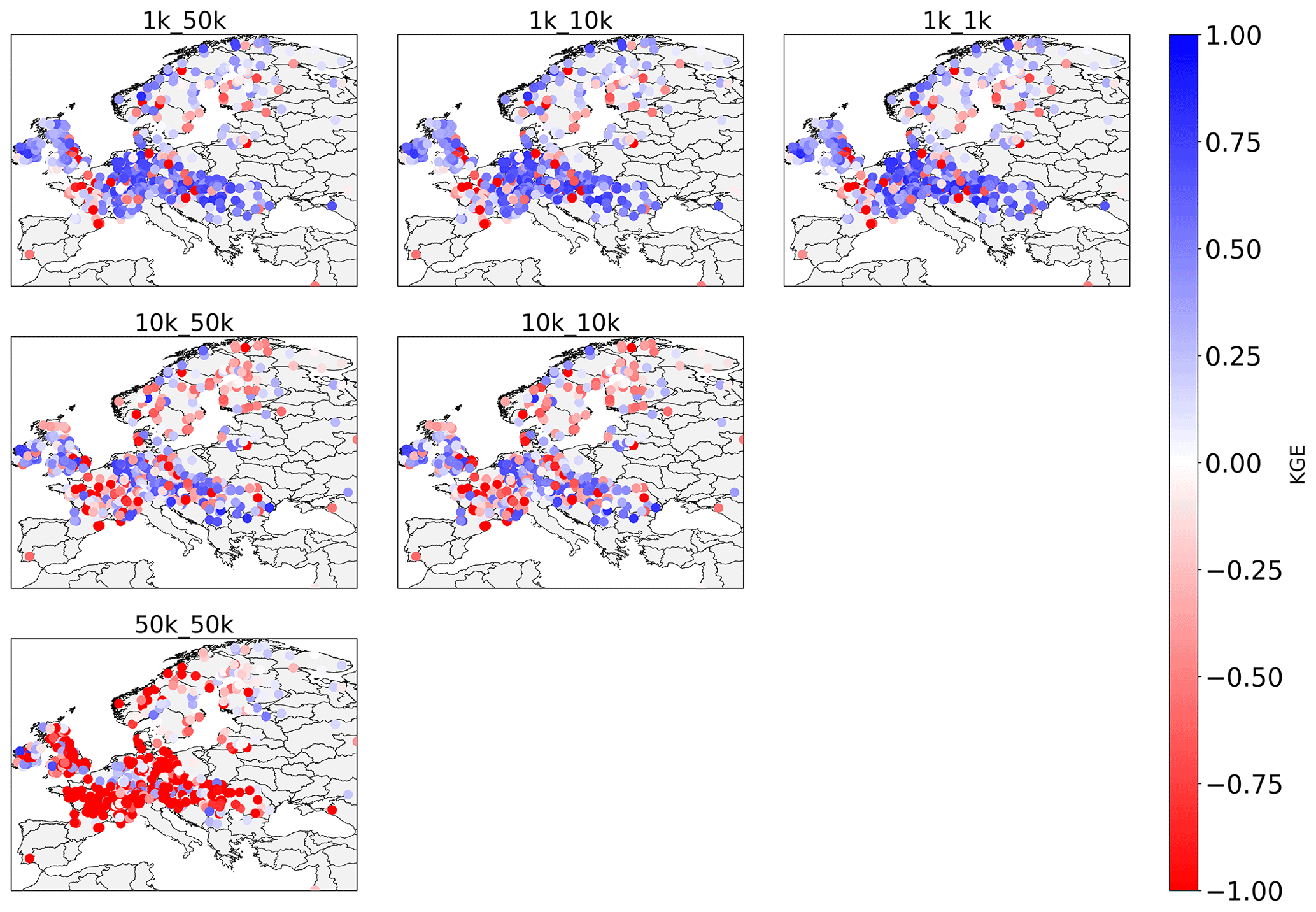
Figure 1KGE values of all selected GRDC stations in Europe.
2.2.2 Upper soil moisture
For validating the average soil moisture of the upper layer, we compare simulations with remotely sensed ESA-CCI (European Space Agency Climate Change Initiative) soil moisture data v06.1 (Dorigo et al., 2017; Gruber et al., 2019). The native temporal resolution is daily, and the spatial resolution is 0.25∘ (roughly 25 km at the Equator). It is noteworthy that the observed data are representative of the upper 5 cm of the soil column, whereas the simulated upper soil moisture from PCR-GLOBWB is an average of the first 30 cm. It is also due to this difference that applying the KGE across all evaluated variables is not feasible. It should additionally be mentioned that an older version of ESA-CCI soil moisture data is one of the input data sources for the GLEAM (Global Land Evaporation Amsterdam Model) evaporation data (see Sect. 2.2.3). Nevertheless, we can still use the ESA-CCI data as an indicator of actual soil moisture dynamics. By computing the spatial mean per water province per time step for both observation and simulation, the resulting time series were used to derive the relative root square mean error (RRMSE) per water with the subsequent equation:
Here, RMSE(obs, sim) is the root square mean error between the observation and simulation time series, and σ(obs) is the standard deviation of the observation time series.
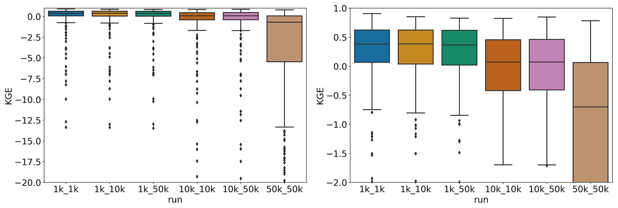
Figure 2Box plot of KGE values obtained for all runs. The plot on the right has been magnified to show a smaller range of values.
2.2.3 Total evaporation
Evaporation makes up a significant factor in the terrestrial water cycle and water balance, strongly determining water availability. Accurate simulation of evaporation is therefore paramount. Unfortunately, there is only little independent observation data available with sufficient temporal and spatial variation and extent.
Therefore, to benchmark the simulated total evaporation per water province, we used data from the remote-sensing-based dataset GLEAM version 3.5a (Miralles et al., 2011; Martens et al., 2017), covering the period from 1980 to 2020. GLEAM v3.5a has a native monthly temporal resolution and a spatial resolution of 0.25∘ (∼25 km). Since the algorithms implemented in GLEAM aim much more at correctly simulated evaporation than PCR-GLOBWB, and because GLEAM employs different (remotely sensed) input datasets, the choice to use a partly model-based benchmark is defensible. Similar to the upper soil moisture evaluation, the RRMSE was determined per water province.
2.2.4 Terrestrial water storage anomaly
By validating the model total water storage against remotely sensed terrestrial water storage, it is possible to evaluate the model's storage dynamics. As such, it provides a more holistic validation including the entire hydrological system state.
Here, a simulated terrestrial water storage anomaly was validated against JPL TELLUS GRACE/GRACE-FO (Kornfeld et al., 2019) data for the period 2002 until 2019. While the native spatial resolution of the data is at 3∘, the data used here are at 0.5∘. Again, monthly averages were computed for both observation and simulations to obtain the RRMSE per water province.
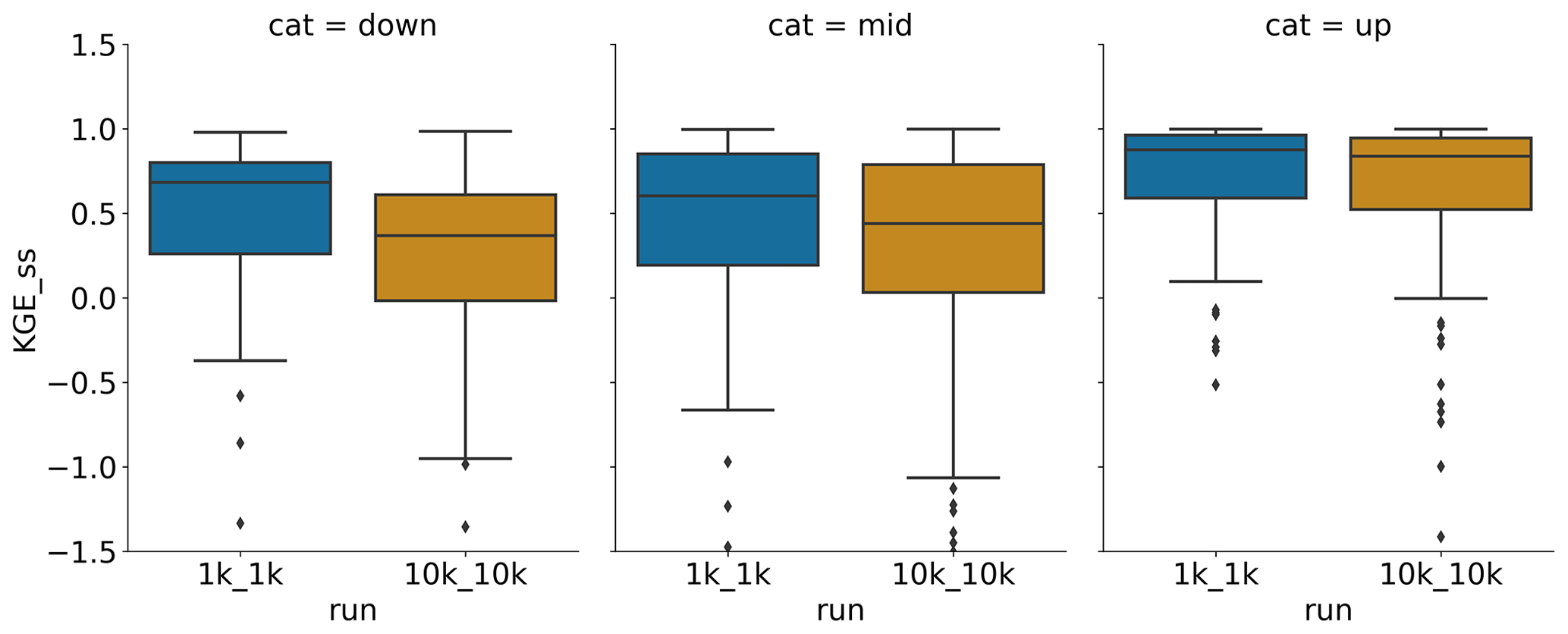
Figure 3Box plots of obtained KGEss values for all stations categorized as downstream, midstream, and upstream for selected runs.
3.1 Simulated discharge
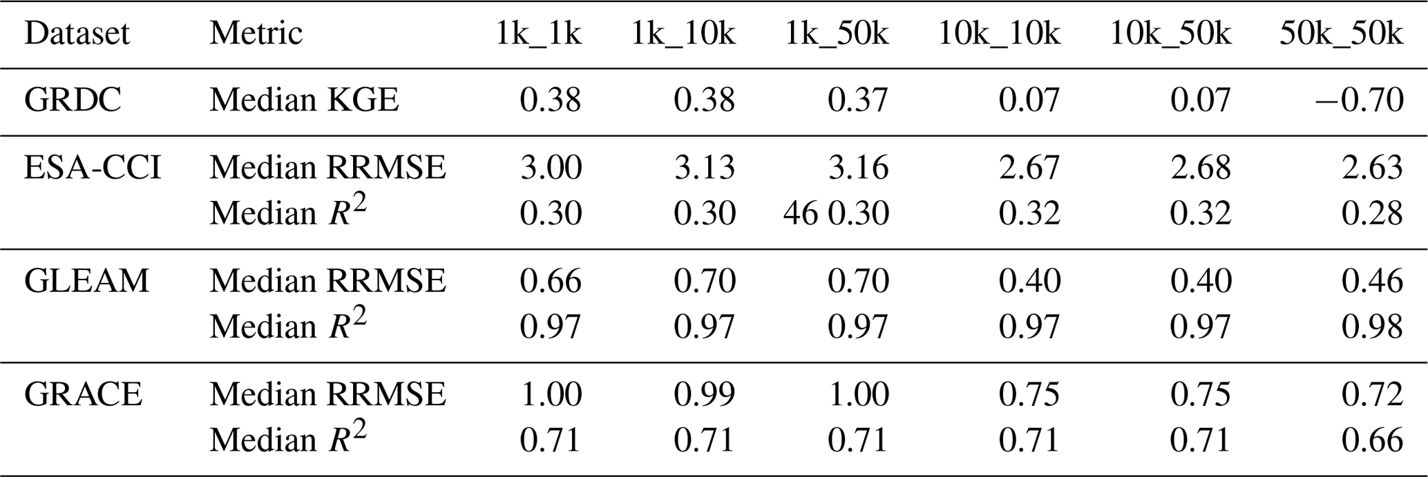
We see that simulated discharge, as expressed by the KGE value averaged over all GRDC stations per water province, improves greatly with a finer model spatial resolution (Figs. 1, 2; Table 2). While the 50k_50k run yields negative median KGE values, this picture improves for finer resolutions, with the 1k_1k and 1k_10k runs comfortably exceeding the accuracy threshold of −0.41, as defined by Knoben et al. (2019). Higher skill with finer resolution is in line with previous research (Altenau et al., 2017), although this should not be expected to be the case for all stations due to locality effects in the scaling process (Aerts et al., 2022). As in our case, only around 7 % of all stations do not show an improvement at all, but roughly 70 % of the stations receive their highest KGE values for the 1k_1k run (Fig. B1). The results nevertheless indicate a robust relation between model resolution and the accuracy of simulated discharge.
The results furthermore indicate that the impact of forcing spatial resolution is present but limited to the 1 K runs, and even there, only the distribution of KGE values contains slightly higher values (as expressed by the whisker extents in Fig. 2), while the mean KGE values are close to identical. Overall, the results suggest that the model resolution is a more important determinant of the accuracy of simulated discharge. Due to the minor differences found across forcing resolutions, the subsequent discharge analyses focus on results from the 1k_1k, 10k_10k, and 50k_ 50k runs.
When analysing results per catchment area category, they also show that the KGE values increase when moving to 1 km hyper-resolution, with the magnitude of improvement depending on the upstream area (Fig. 3). In line with previous results and our hypothesis, employing finer resolutions than the reference 50 km has the most pronounced effect at upstream locations, where the 50 km model is seemingly less capable of reproducing observed discharge. For midstream and downstream stations, KGEss values show the greatest improvement for the 1k_1k run and hence a clear beneficial effect of hyper-resolution hydrological modelling. In fact, simulated discharge at 1 km improves over either 10 or 50 km or both at around 93 % of the GRDC stations assessed (see Fig. B1). In addition to our hypothesis that hyper-resolution is beneficial in upstream areas, these results suggest that a better representation of smaller streams contributes to more accurate discharge simulations at large scales.
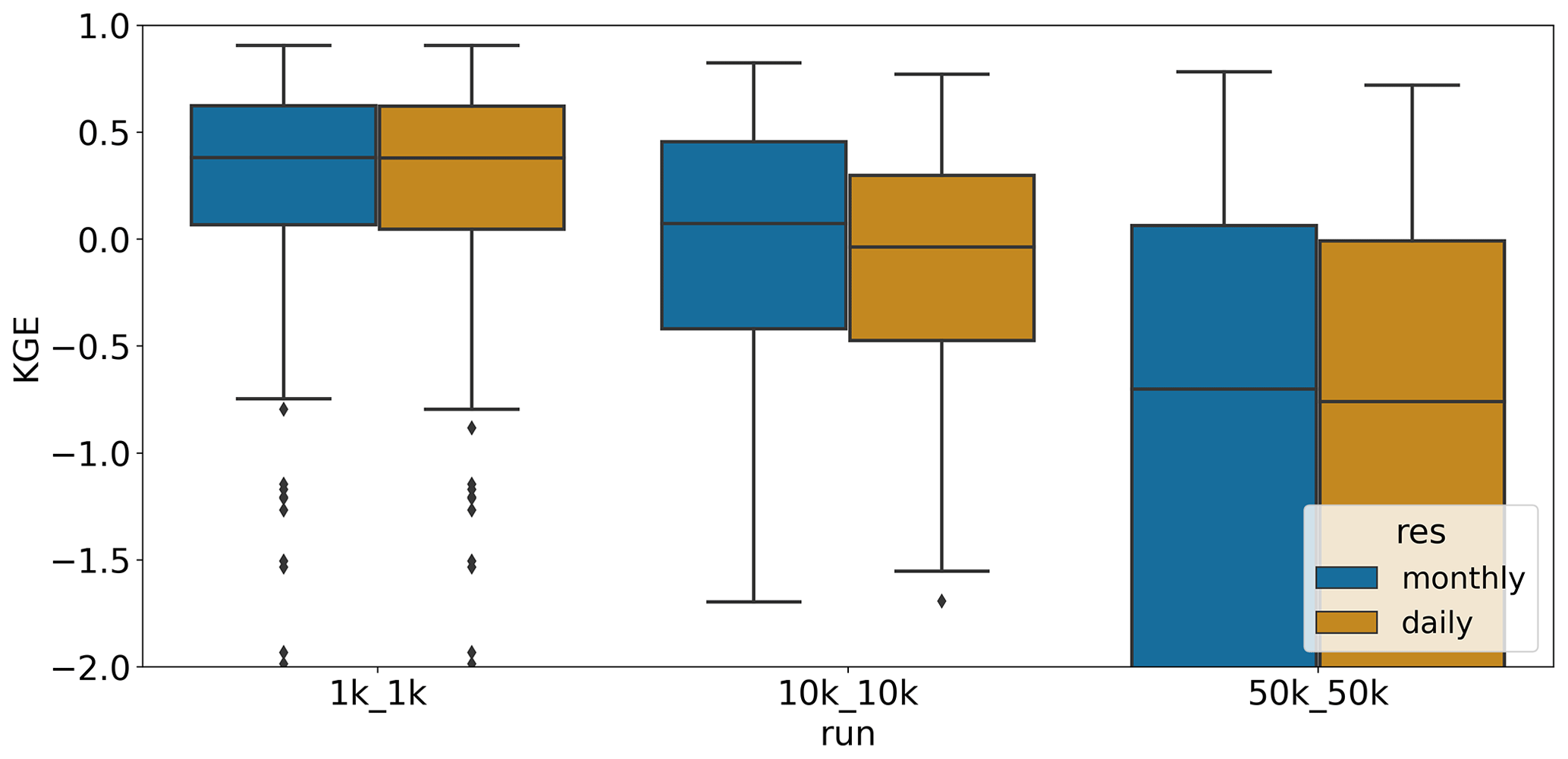
Figure 4Comparison between KGE distribution presented as box plots for the different spatial resolution and temporal resolution of the discharge output.
Another hypothesis we tested is whether the accuracy of fast processes simulated at daily resolution, such as discharge generation, improve compared to longer aggregation periods, for example months, with finer spatial resolution. This is in line with Melsen et al. (2016), who argue that “the calibration and validation time interval should keep pace with the increase in spatial resolution”. Based on Fig. 4, this hypothesis cannot be confirmed for the PCR-GLOBWB model. We do, however, want to stress that these results do not mean that moving to hyper-resolution does not yield improvements for shorter temporal intervals at all. It is highly likely that the simplistic routing schematization used in this experiment limits the improvement of daily discharge dynamics. Using more advanced routing schemes was not feasible due to the resulting high computational demand. It can thus be assumed that the daily discharge estimates presented here do not fully represent the potential benefits which could be achieved with hydrological simulations at hyper-resolution.
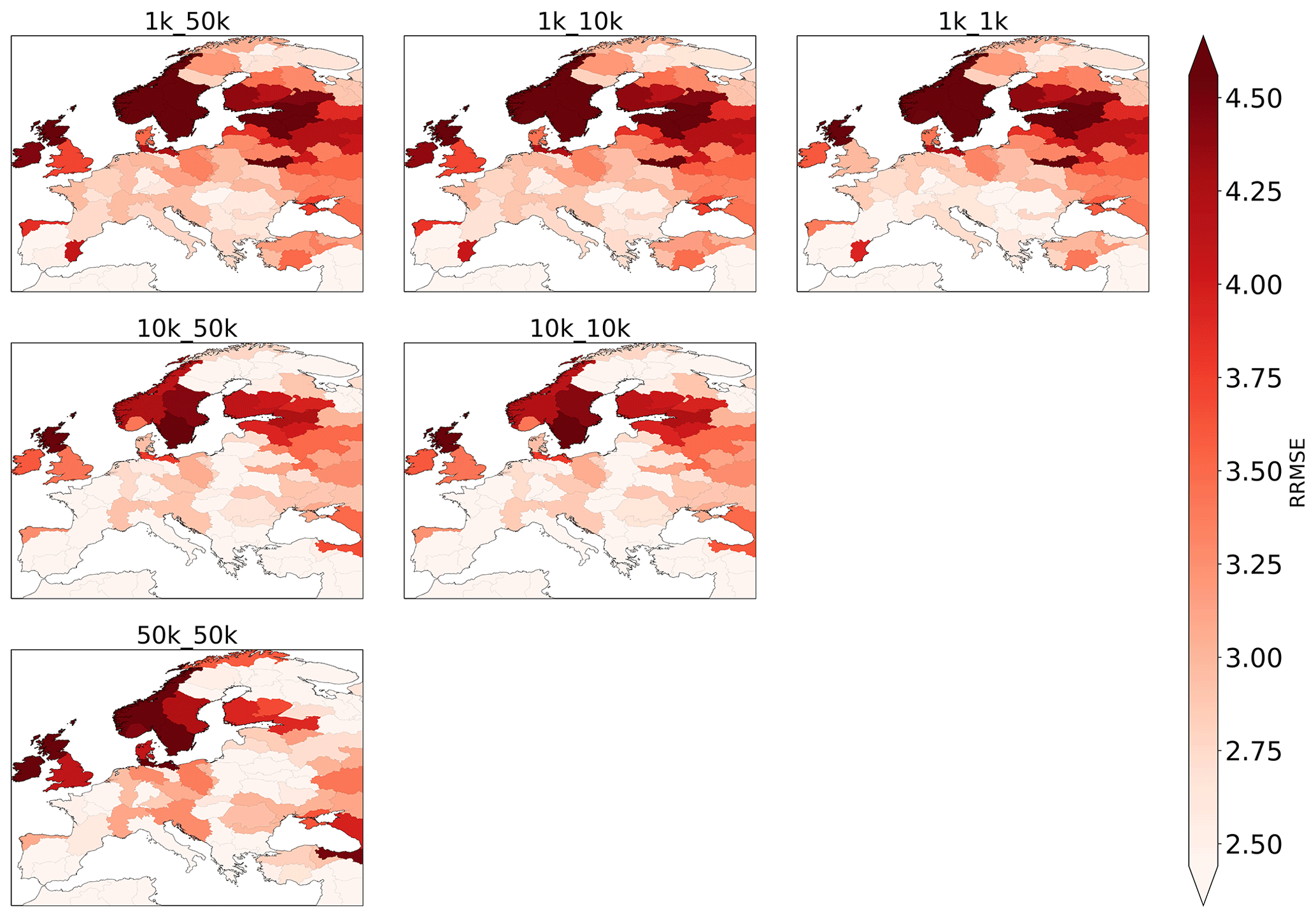
Figure 5Relative root mean square error (RRMSE) values computed per water province based on simulated upper soil moisture and observations from ESA-CCI.
3.2 Upper soil moisture
To assess the model skill in reproducing upper soil moisture, we analysed RRMSE values obtained per water province (Fig. 5). Overall, we find areas with consistently low and high RRMSE values. Particularly the UK, Ireland, southern Sweden and Norway, the Rhine–Meuse delta, and a larger area centred around Austria have high RRMSE values. Large parts of Spain, Portugal, and Finland, as well as northern Sweden, show overall good model performance, as indicated by low RRMSE values.
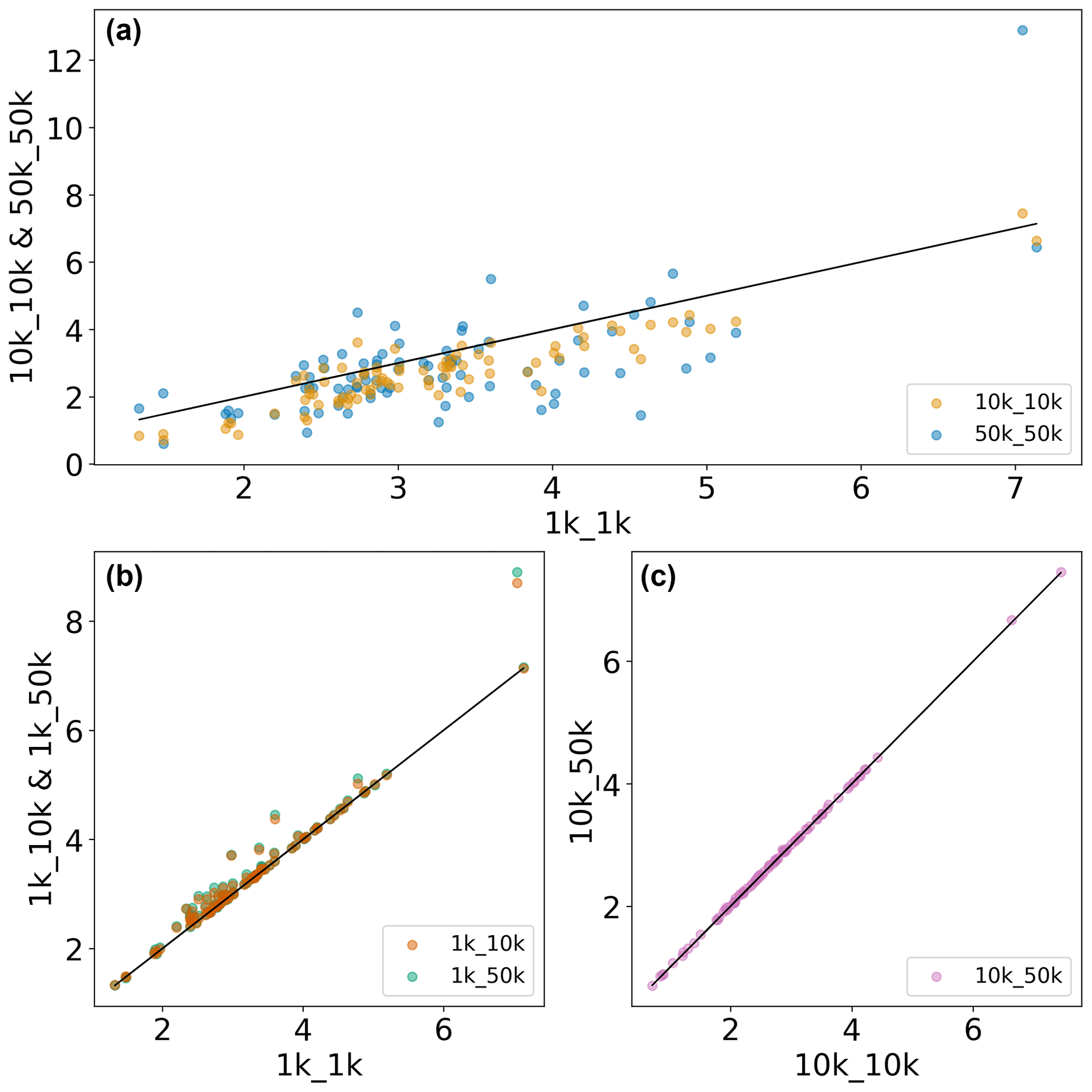
Figure 6Scatterplot of RRMSE values obtained in the evaluation of simulated upper soil moisture with ESA-CCI data for (a) comparing different model resolutions, (b) comparing different forcing resolutions for 1 K runs, and (c) comparing different forcing resolutions for 10 K runs.
Comparing RRMSE values across both model resolutions (Fig. 6a and Table 2) reveals that the 10 K runs, when benchmarked against the 1 K run, produce overall lower RRMSE values and are thus more accurate, although differences between median values are small overall, especially between the 1k_1k and 10k_10k runs. It is in line with our expectations that the 50 K run has the highest RRMSE values. Figure 6b and c compare RRMSE values across forcing resolutions, indicating that employing a coarser forcing resolution decreases model accuracy for the 1 K runs while not having significant impact on the 10 K run (see also Table 2) – a similar pattern to that found in the discharge evaluation.
It should be noted, however, that observed and simulated soil moisture values are based on different soil depths, which may have a not-further-quantifiable impact on analysis results. The fact that a similar pattern is found when assessing time series variability as expressed by the coefficient of determination R2 indicates that the relation between observation and simulations is also well represented when assessing RRMSE values (Fig. B2).
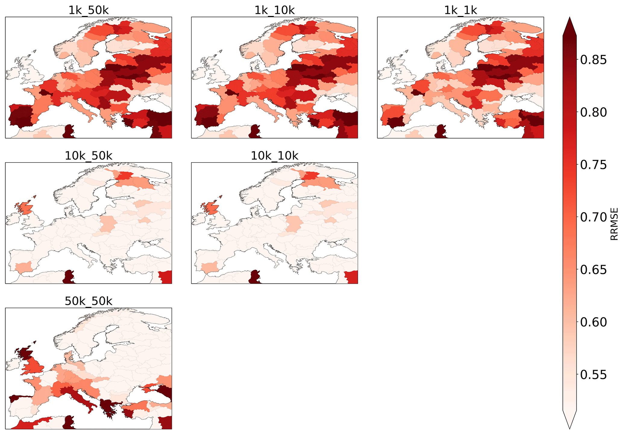
Figure 7RRMSE values computed per water province based on simulated total evaporation and evaporation data from GLEAM.
Ranking the accuracy of the runs by their mean RRMSE value, we see that the 10 K runs perform best, followed by the 1k_1k run (Table 2). The fact that the 10k_10k runs clearly outperform the 1k_10k and 1k_50k runs indicates that a forcing resolution that is too coarse can eradicate the potential benefits of finer model resolution and that employing a coarser model resolution with a (relatively) fine forcing resolution may lead to similar accuracy.
3.3 Total evaporation
Results indicate that model accuracy is lowest for the 1 K runs, followed by the 50 K run (Figs. 7, B3a; Table 2). The 10 K runs show the best performance overall in resembling evaporation estimates from GLEAM. We furthermore find that RRMSE values are smaller and range between 0.22 and 1.78, indicating an overall better agreement between the simulation and observation than for surface soil moisture. The deterioration of model accuracy at 1 km scale is visible over the entire European continent, except for Great Britain, where we see an improvement when moving towards 1 km model resolution.
In line with the soil moisture evaluation, employing a coarser forcing resolution increases RRMSE values for the 1 K runs, and hence decreases model accuracy, but has no impact on the 10 K runs (Figs. B3b, c; Table 2).
3.4 Terrestrial water storage anomalies
As with all previous evaluations, evaluating terrestrial water storage (TWS) anomalies indicates that coarser forcing resolutions yield reduced model accuracy, but in this case, the impact is smaller than for previously assessed variables (Fig. B4b, c; Table 2).
Figure 8 shows that there are distinct hotspots (Scandinavia, the UK and Ireland, Italy, and water provinces along the Atlantic and Mediterranean coast) where model accuracy is limited, regardless of the model resolution or forcing resolution employed. Furthermore, the same pattern occurs as with total evaporation, namely that overall RMSE values are lowest for model resolutions coarser than 1 km (in that case, the 50 K run; Fig. B4a; Table 2). These findings, again, may be related to the fact that the large original footprint of the GRACE data of 3 arcmin or roughly 300 km cell length, despite downscaling it to 0.5∘, favours coarser resolutions. In fact, the match in spatial resolution may be explaining some of the good performance of the 50 km run. Consequently, the (potentially) added value of finer model resolutions may not be captured when using GRACE data for evaluation.
Table 2Overview of median evaluation metrics per run per evaluated variable except for discharge.
4.1 Model parameterization
In the debate of hyper-resolution, the role of model parameterization is a major topic. Here, we did not attempt to improve model parameterization or replace parameterized processes with empirical scaling relations when moving from coarse to fine resolution. This allows us to make inferences about the importance of scale-consistent model parameterization and where using the (thus far) default approach (simple parameter upscaling and changing forcing resolutions) may reach its limits.
As an example, we assessed in more detail the parameterization for the groundwater response times, which has a major impact on groundwater storage dynamics. Our hypothesis is that it needs to be adjusted for finer spatial resolutions as it does not (yet) correctly scale with the underlying drainage network and therefore results in the lower accuracy when evaluating TWS anomalies of the 1 km runs (Sect. 3.4). Consequently, model response, particularly with respect to regional groundwater dynamics, may be too slow at model resolutions finer than the (thus far) default 10 km resolution, and hence, the groundwater response is out of sync with observations. A lower correlation (expressed here as the coefficient of determination R2) may thus result in high RRMSE values. To further analyse this, we categorized each water province according to its R2 and RRMSE values (Fig. 9). Indeed, results suggest that R2 is an overall good predictor of RRMSE because water provinces with a high R2 tend to have low RRMSE values, and vice versa, accounting for a total of 66 % to 68 % of all provinces across all runs. More important is that, for the 1 km run, we find the greatest median RRMSE value. Consequently, issues related to the correct scaling of the recession parameter may indeed contribute to the lack of improvement at finer model resolutions.
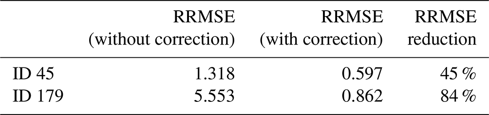
Another example is the question of whether using a parameter or equation can affect the model accuracy with the accumulation of water storage over time, particularly in snow-dominated areas, where the downscaled temperature at 1 km is mostly below the freezing point. Again, such an accumulation decreases the model accuracy of the simulated TWS anomalies. In these areas, PCR-GLOBWB does not yet contain enough physical processes to redistribute snow to other 1 km cells (e.g. glaciers or avalanches). Indeed, correcting for snow cover in the 1k_1k run had a positive effect when evaluating TWS anomalies (Table 3) for two water provinces (not surprisingly located in and around the Alps; see Fig. B5), strongly suggesting that the current approach to calculating snow cover and the changes thereof may locally limit the model accuracy for hyper-resolution runs.
4.2 Scale commensurability of simulated and observed data
Scale commensurability is an important aspect when comparing simulated and observed data when (in)validating a model (Beven et al., 2022). In line with previous research (Gleeson et al., 2021), commensurability errors are reduced for increasingly finer spatial resolutions, which translates to more accurate river networks, and in turn less spatial aggregation, when evaluating simulated discharge.
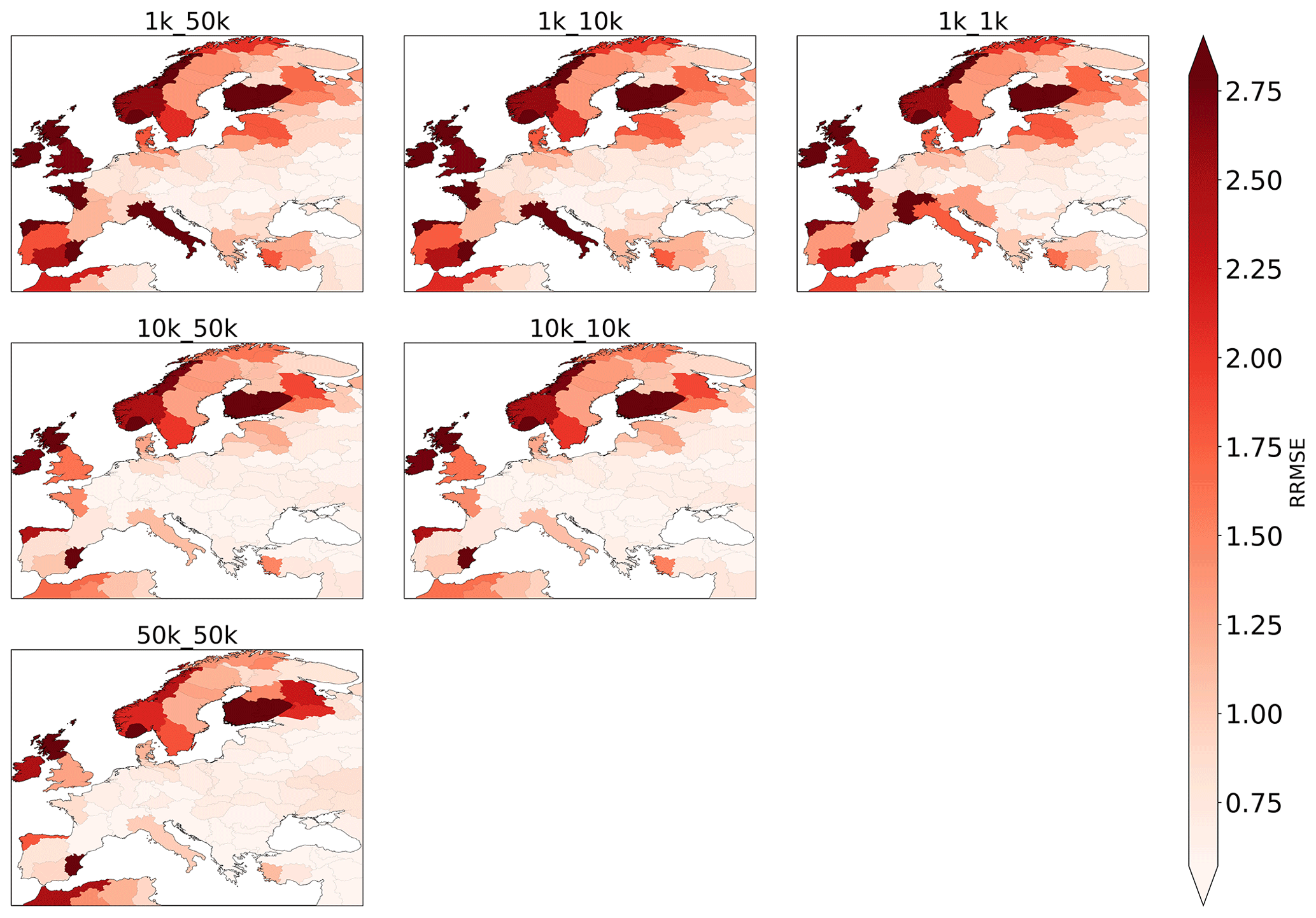
Figure 8RRMSE values computed per water province based on simulated total water storage anomalies and terrestrial water storage anomalies from GRACE/GRACE-FO.
For most of the other evaluated variables, however, results tend to be favourable for coarser model resolutions. A clear answer to what causes these ambiguous results is currently, however, not possible, as the epistemic uncertainty is large with the observations, the model schematizations derived at coarser resolutions from the default 1 km model data, the mismatch in spatial resolutions between observations and model, or all of the above may lead to mixed results, and additional efforts need to be taken to reduce this uncertainty.
Currently, the difference between the finest resolution of the model (1 km) and of observational datasets that cover the entire European domain and have a sufficiently long record (25 to 50 km) is undoubtedly great. However, as only recent satellite missions, such as the ESA Sentinel mission or commercially driven ones, can produce data at the (sub-)kilometre scale, it will still take some time until the observed period is sufficiently long for robust long-term model evaluations. For example, surface soil moisture data collected by Sentinel-1B started in 2015 only, whereas the ESA-CCI data used here covers the period from 1978 to 2020. Similarly, MOD16A ET data provide sub-kilometre-scale evapotranspiration data starting in 2001. Even though this is already a longer track record, it would mean disregarding 20 years of simulations, which may be too short for establishing a baseline understanding of the effect of hyper-resolution.
Table 3RRMSE values for two selected water provinces without and with correction for snow cover when evaluating simulated TWS anomalies.
4.3 Computing and data storage demand
Another important aspect of hyper-resolution hydrological modelling is the computational demand and the numerical scheme used. Table 4 shows the computational demands for different model resolutions using the Dutch National Supercomputer Snellius. Without parallelization, the wall clock time for a 10 km run was about 36 h. This entails that the 1 km model, having the size of about 100 times the 10 km model, would result in a wall clock time of 3600 h (∼150 d). This wall clock time is clearly not viable, and therefore, the 1 km model was run in parallel for 45 chunks.

Figure 9Plot of R2 and RRMSE values per water province, categorized in four quartiles based on their median R2 and RRMSE values, respectively, for 1k_1k, 10k_10k, and 50k_50k runs (from left to right). Values in the corners of the quartiles represent the fraction of data points in the respective quartiles.
Table 4Overview of indicators for computational demand of the runs at different model resolutions. The file sizes refer to output for one variable.
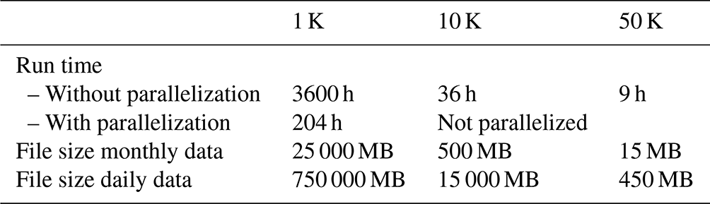
As the underlying numerical scheme of PCR-GLOBWB has not been changed for computationally more demanding hyper-resolution simulations, it is clearly sub-par. Besides using ever more powerful high-performance computers (HPCs), additional efforts should be taken to improve model parallelization capacities, as implemented in comparable models (Kollet and Maxwell, 2006; Kollet et al., 2010; Bierkens et al., 2015). Evidently, the challenge of hyper-resolution hydrological modelling is not only one of data and parameters but also one of model design, which needs to follow the most recent software and hardware developments such as, for instance, distributed memory parallel modelling (Verkaik et al., 2021, 2022), asynchronous many tasks (de Jong et al., 2022, 2021), or running the simulations on GPUs (Shaw et al., 2021) or XPUs (cross-architecture computing solutions) in general.
Once shorter run times are achieved, it can have direct positive effects on model results too, especially discharge. With the (thus far) default model design, we had to employ the accuTravelTime routing scheme, the largest simplification of the shallow water equations. This renders particularly the daily discharge simulations potentially inaccurate and does not make full use of a hyper-resolution river network, as relevant physical processes are not included. Once a speed-up of the model is realized by considering one of the abovementioned options, it could be feasible to employ more sophisticated versions of the shallow water equations. But, also for other model variables, an improved numerical scheme will be crucial when processes replace the parameterization at 1 km resolution.
In this study, we assessed challenges and opportunities of refining both the model and forcing spatial resolution from 50 to 10 km to a hyper-resolution of 1 km, aiming to increase our understanding of scale dependencies of both the model and the meteorological input. Our work shows that a forcing resolution that is too coarse can eradicate the benefits of the model hyper-resolution. Hence, if forcing is only available at a coarse spatial resolution, then applying a hyper-resolution model will not provide any performance gain and only increase the computational demand. Furthermore, results show that model resolution is greatly defining the overall output accuracy because if model skill at a given model resolution and coarse forcing resolution is already low (or high), then employing a finer forcing resolution will only yield limited improvement. Consequently, future work should be aimed at advancing both model and forcing data. For the latter, the scale gap between currently achievable model resolution and available meteorological datasets needs to be closed.
Even though the hyper-resolution model presented here is not just the same old model with more grid cells but populated with as much high-resolution parameter data as possible, there is still room for model improvement. Currently, the used parameterization design is not fully scalable from the current default of 10 to 1 km. Clearly, some parameters or sub-grid approaches should be replaced by actual data when moving to hyper-resolution. As exemplified in Sect. 4.1, the model accuracy at 1 km spatial resolution may be lower than necessary due to an unfit model parameterization. Considering the growing number of openly available datasets, it is necessary to carefully review the model parameters and their values currently used. In some instances, it may be better to include additional physical processes to capture the immense natural heterogeneity which can be resembled at the 1 km scale (Clark et al., 2017; Beven and Cloke, 2012), while making sure that including these processes and fine-scale data results in consistent parameterizations across scales (Samaniego et al., 2010). It is only when the model parameterization is improved and more processes are implemented at hyper-resolution that the full potential of a hyper-resolution model grid can be employed. Then, we expect that model realism will improve and epistemic uncertainty will decrease, leading to improved accuracy overall.
While a finer model resolution has a clear positive effect on simulated discharge, answering the question of scale commensurability when employing long-term observational datasets with coarse spatial resolutions remains challenging (see Sect. 4.2). Following up on the baseline study presented here, a second step in (in)validating the simulated results is recommended in which finer-resolution observational data should be employed to reduce the scale-related commensurability uncertainties (Beven, 2018, 2016). The availability of a 1 km model output over large extents now offers a great opportunity to make full use of the benefit of these novel data. In that context, the need to use water provinces to link across spatial resolutions could be lifted when merely assessing hyper-resolution model output, thus allowing the model evaluation to be performed at the individual grid scale.
As discussed in Sect. 4.3, performing hyper-resolution simulations is still pushing the boundaries of what is currently possible. Despite advances made in both software and hardware acceleration, access to high-performance computers with sufficient CPU, memory, and disk space remains vital for hyper-resolution simulations at the continental scale, let alone for global application. Democratizing this access will therefore be crucial to enable researchers worldwide to advance hyper-resolution hydrological modelling. Additionally, the numerical scheme of any model attempting continental-scale hyper-resolution simulations needs to be on par with the task at hand. This is not to say that all models need to be refactored entirely, but undoubtedly optimized code and some form of advanced cyber infrastructure (Condon et al., 2021) needs to be in place – possibly supported by research software engineers (Hut et al., 2017) – to deal with the high storage and computational demand of not only running the simulations but also storing both input and output data in addition to analysing the results.
All in all, the results presented here should not be considered the final outcomes of a development towards global hyper-resolution hydrological modelling. Instead, they are rather a first effort to map both opportunities and challenges of continuous simulations at 1 km resolution over large extents, with lessons learnt for iterative open-ended model evaluation and the subsequent improvement of model parameterization and configuration (Gleeson et al., 2021; Bierkens et al., 2015). Since the study here is at the continental scale (yet with global model configurations and global datasets), the findings made should be confirmed (or disregarded) in a global-scale study, ideally using high-resolution observation datasets for benchmarking. Now that a modelling and evaluation workflow is established, the threshold for performing such a study is lowered. Since most hyper-resolution studies are done over data-rich regions, it will be revealing to see how the hyper-resolution models perform over data-scarce areas. As such, the results here should be seen as first steps in the realm of hyper-resolution with many more to follow.
Despite the currently limited availability of observation dataset at matching spatial resolution and the still very demanding computations, we share the positive outlook of O'Neill et al. (2021) and are convinced that on-going data collection efforts, advanced satellite missions, and ever-powerful computers will eventually result in hyper-resolution becoming the default in the foreseeable future and in turn provide globally continuous yet locally relevant results.
For more extensive details, we refer to previous PCR-GLOBWB model studies, particularly the ones at 50 km resolution (van Beek et al., 2011; van Beek, 2008; van Beek and Bierkens, 2008) and 10 km resolution (Sutanudjaja et al., 2018), in addition to 1 km resolution (Sutanudjaja et al., 2011).
A1 Meteorological forcing
As the meteorological forcing input, PCR-GLOBWB requires daily spatial fields of precipitation and temperature, in addition to reference potential evaporation. For this study, reference potential evaporation is calculated using the Penman–Monteith method, following the FAO guidelines (Allen et al., 1998) that requires net radiation, wind speed, and vapour pressure deficit (see van Beek, 2008, for details).
For all of the aforementioned required meteorological fields, we downloaded the ERA5-Land dataset (Muñoz-Sabater et al., 2021), which is provided at 6 arcmin and hourly resolution. We then resampled the ERA5-Land precipitation and temperature variables to daily spatial fields at 5 arcmin resolution so that they can be used for our 10 km model runs. We also resampled the required variables for the reference potential evaporation calculation at 5 arcmin resolution and used it as the reference potential evaporation input of our 10 km model runs.
For our 50 km model run, we upscaled or averaged the 5 arcmin daily precipitation, temperature, and reference potential evaporation variables to their 30 arcmin daily fields. For 1 km model runs, we downscaled the daily precipitation and temperature fields from 5 arcmin to 30 arcsec, using the monthly lapse rate fields from Sutanudjaja et al. (2018). We refer to Sutanudjaja et al. (2011) for more details about the downscaling procedure. The downscaled 30 arcsec temperature fields were also used to calculate the reference potential evaporation fields based on the Hamon (1963) method that requires only daily mean temperature as its input. We then used these Hamon (1963) 30 arcsec fields to downscale the 5 arcmin fields of the Penman–Monteith reference potential evaporation to 30 arcsec resolution.
A2 Land surface: soil, and cover, and topography
For soil parameterization, the maps from SoilGrids250 (Hengl et al., 2017) were used in this study. This is different to previous PCR-GLOBWB studies that used the Digital Soil Map of the World (DSMW; FAO, 2007). An obvious advantage of using SoilGrids250 comes from its sufficiently fine resolution at 0.002 arcdeg resolution (0.12 arcmin; about 250 m at the Equator), while DSMW may not be suitable for model grids finer than 5 arcmin resolution (see e.g. Batjes, 2012).
The PCR-GLOBWB model cannot directly use the soil information of SoilGrids250, which not only has a finer spatial resolution than 1 km PCR-GLOBWB but also specifies only some general attributes such as soil texture. Here we transformed these attributes of SoilGrids250 into soil hydraulic properties, such as the water-holding capacity, field capacity, and wilting point, using the pedotransfer functions from Balland and Arp (2005) and Balland et al. (2008). These pedotransfer functions allow the estimation of bulk density and related soil hydraulic properties at any given depth, which is required to link the layer information from SoilGrids250 to the two-layer schematization in PCR-GLOBWB. We derived these soil properties at the spatial resolution of 0.002 arcdeg and subsequently upscaled and resampled them to the various coarser PCR-GLOBWB model resolutions used in this study, i.e. 30 arcsec (∼1 km at the Equator), 5 arcmin (∼10 km), and 30 arcmin (∼50 km).
For the standard parameterization of the land cover the following datasets were combined, namely the map of Global Land Cover Characteristics (GLCC) database version 2.0 (Loveland et al., 2000), with the land cover classification following Olson (1994a, b) and the parameter sets from Hagemann et al. (1999) and Hagemann (2002). For the extent of irrigation areas, the map of Global Food Security Support Analysis Data (GFSAD) version 1.0 (Teluguntla et al., 2016) was used. The GLCC and GFSAD maps are available at 30 arcsec resolution (∼1 km). Hence, for 1 km model runs, only one land cover type exists per cell. For the resolutions of 10 and 50 km, land cover types were divided into four land cover types consisting of tall natural vegetation, short natural vegetation, non-paddy-irrigated crops, and paddy-irrigated crops (i.e. wet rice). Irrigation land cover types (i.e. paddy and non-paddy), including their crop calendars and growing season lengths, were parameterized based on the dataset of MIRCA2000 (Portmann et al., 2010) and the Global Crop Water Model (Siebert and Döll, 2010). A detailed description can be found in the key PCR-GLOBWB model description literature (Sutanudjaja et al., 2011, 2018; van Beek et al., 2011).
For topographical-related input, we made use of the state-of-the-art Multi-Error-Removed Improved-Terrain Hydro digital elevation model (MERIT Hydro DEM; Yamazaki et al., 2019) that is available at 3 arcsec resolution (∼90 m at the Equator). This is different to the previous PCR-GLOBWB studies (Sutanudjaja et al., 2018; van Beek et al., 2011) that used previous-generation DEM datasets, such as HydroSHEDS (Lehner et al., 2008) or GTOPO30 (Gesch et al., 1999). The 3 arcsec MERIT Hydro DEM was upscaled to the resolutions of 30 arcsec (1 km), 5 arcmin (10 km), and 30 arcmin (50 km). Yet, we also used its original 3 arcsec resolution elevation values to obtain several sub-grid variability parameters that influence various schemes in PCR-GLOBWB, such as runoff-infiltration partitioning, interflow, groundwater recharge, and capillary rise, as well as evaporation processes (van Beek, 2008; van Beek and Bierkens, 2008; Hagemann and Gates, 2003; Todini, 1996).
A3 Groundwater
In PCR-GLOBWB, groundwater discharge (also commonly known as groundwater baseflow) depends on a linear storage–outflow relationship, in which a groundwater recession coefficient field is calculated following the drainage theory of Kraijenhoff Van de Leur (1958), which is based on the drainage network density and aquifer properties. For the drainage density, we used the estimate from van Beek and Bierkens (2008). The aquifer properties were estimated from the GLobal HYdrogeology MaPS (GLHYMPS) dataset of Gleeson et al. (2014). These datasets are reasonable and sufficiently fine for modelling at 1 km resolution and can be upscaled to 10 km resolution and 50 km resolution.
A4 Surface water routing: lakes, reservoirs, and drainage/river network
PCR-GLOBWB also includes lakes and reservoirs that are taken from the Global Lakes and Wetlands Database (GLWD) of Lehner and Döll (2004) and from the Global Reservoir and Dam Database (GRanD) of Lehner et al. (2011). Reservoirs are processed as follows: for every resolution, we rasterize the GranD shapefiles containing information about reservoir surface areas and capacities. During the rasterization process, we need to account for many factors, such as reservoir locations to the drainage networks (at different resolutions) and the number of reservoirs within pixels. If a pixel contains more than one reservoir (which is very likely in coarser resolution), we merged their surface areas and capacities and treated them as one reservoir. Consequently, the overall physical properties of reservoirs should not be overly different when moving from finer to coarser resolutions, and thus their impact of flow estimates can be considered to be small.
For the drainage network maps, we made use of the existing 30 and 5 arcmin maps from Sutanudjaja et al. (2018) and the 30 arcsec one from the HydroSHEDS (Lehner et al., 2008). Note that the MERIT Hydro DEM, which we used as the source of DEM, provides a drainage/river network at 3 arcsec resolution only and, therefore, cannot be used for this study.
In Fig. B1, the improvement of KGE values per station are mapped. To that end, it was assessed whether the KGE value for the 1k_1k run was higher than for either the 10k_10k run or the 50k_50k run, higher for both runs, or not higher at all. The results indicate that KGE values largely improve, with only around 7 % of the stations showing no improvement at all when refining the model resolution.
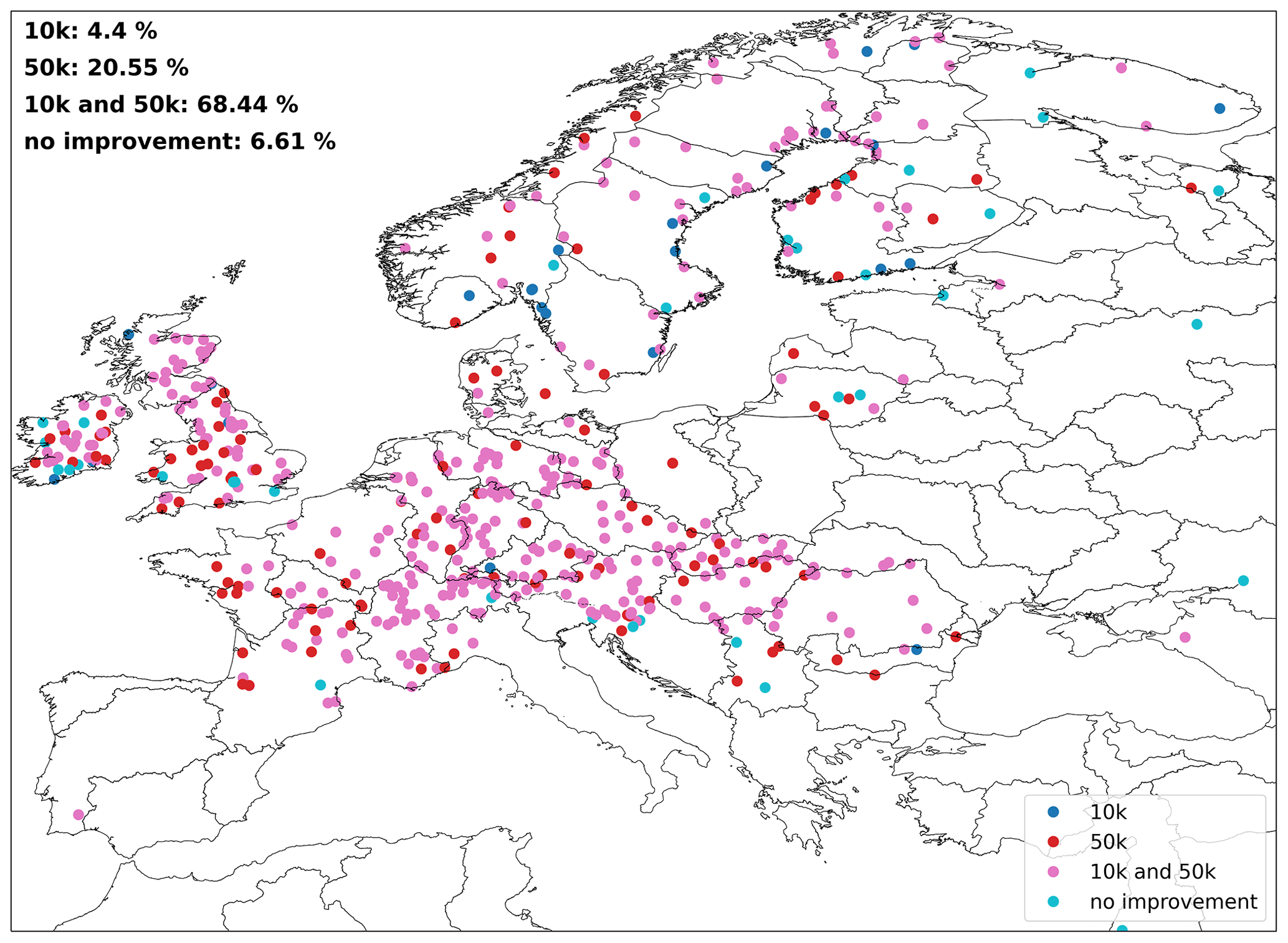
Figure B1Map of stations where the 1 K run showed improvement with respect to only the 10 K run, only the 50 K run, both runs, or none of the runs.

Figure B2Scatterplot of the coefficient of determination (R2) values obtained in evaluation of simulated upper soil moisture with ESA-CCI data for (a) comparing different model resolutions, (b) comparing different forcing resolutions for 1 K runs, and (c) comparing different forcing resolutions for 10 K runs.
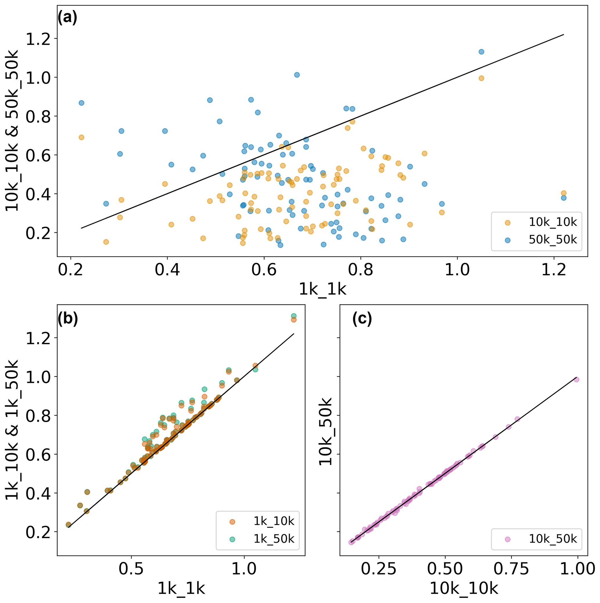
Figure B3Scatterplot of RRMSE values obtained in the evaluation of simulated total evaporation with GLEAM data for (a) comparing different model resolutions, (b) comparing different forcing resolutions for 1 K runs, and (c) comparing different forcing resolutions for 10 K runs.
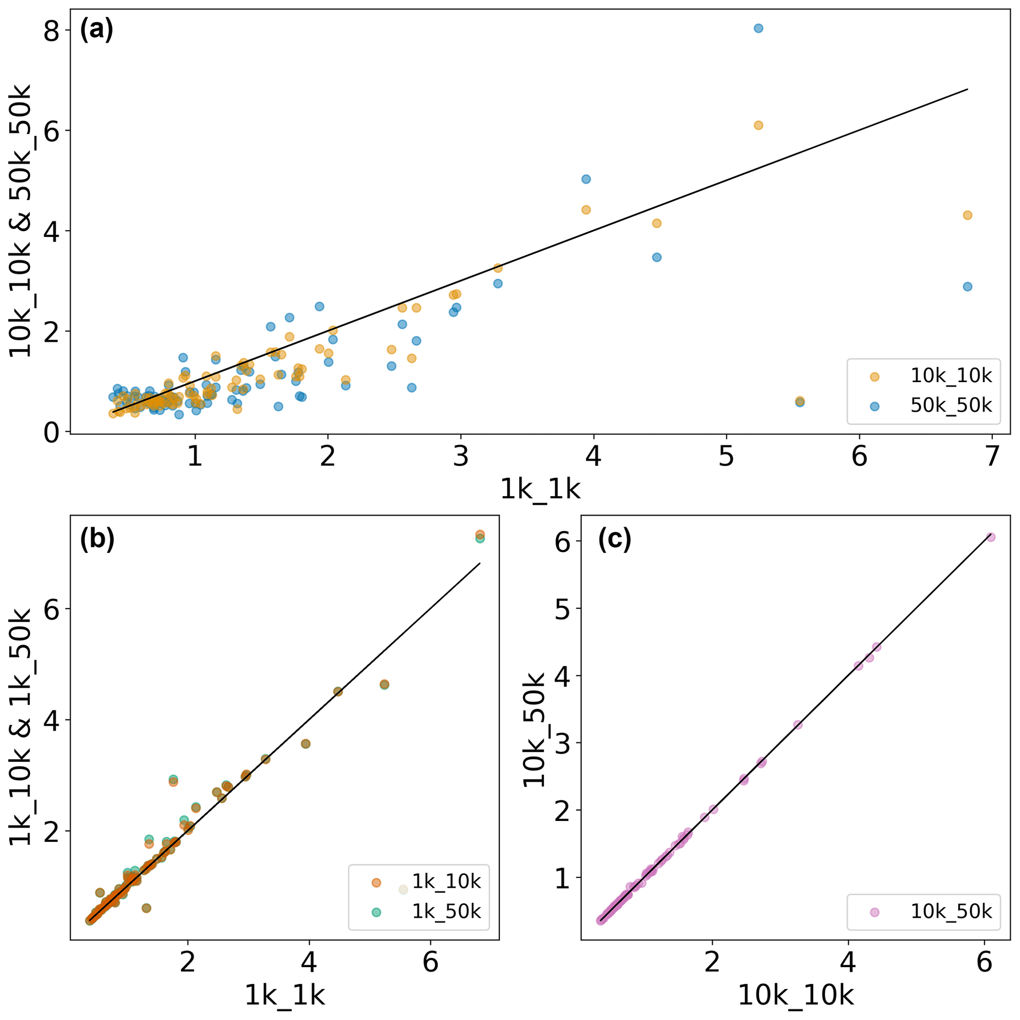
Figure B4Scatterplot of RRMSE values obtained in the evaluation of simulated terrestrial water storage anomaly with GRACE/GRACE-FO data for (a) comparing different model resolutions, (b) comparing different forcing resolutions for 1 K runs, and (c) comparing different forcing resolutions for 10 K runs.
Figures B2–B4 provide scatterplots of R2 and RRMSE values obtained by evaluating various model variables with observational datasets at the water province level. While panel (a) in Figs. B1–B4 compares the impact of different model resolutions (1, 10, and 50 km), panels (b) and (c) compare the impact of different forcing resolutions, including (panel b) 1 km model resolution with 1 km forcing resolution against 1 km model resolution and 10 and 50 km forcing resolution, respectively, and (panel c) 10 km model resolution with 10 km forcing resolution against 10 km model resolution and 50 km forcing resolution.
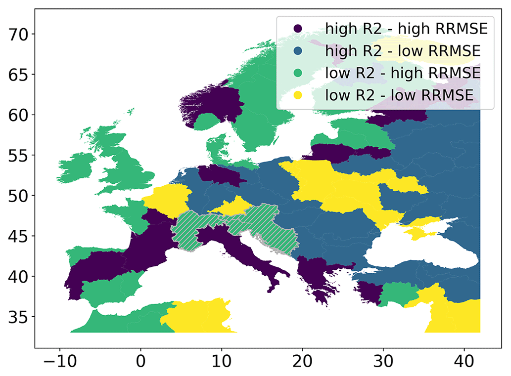
Figure B5Categorization of water provinces according to their R2 and RRMSE values. Grey hatching refers to water provinces for which the snow cover correction of TWS anomaly was effective (see Sect. 3.4).
Figure B5 depicts the categorization of each water province, conditional on their R2 and RRMSE values. Four categories were defined, namely with low and high R2 values and low and high RRMSE values. The median R2 (respectively, RRMSE) value was used to define low and high values. It is shown that there is not really a consistent spatial pattern where one category dominates. Additionally, this figure shows those provinces for which we analysed the impact of removing snow cover in the evaluation of TWS anomalies in Sect. 4.1.
Model output was evaluated using the pcrglobwb_utils package (Hoch, 2021). As the original model output requires a lot of disk space, only the output from the evaluation step is provided under https://doi.org/10.5281/zenodo.6390219. For the original output, please contact the corresponding author.
JMH, EHS, and MFPB designed and supervised the experiment. EHS prepared the model data and performed the analyses, with critical feedback from all co-authors. JMH developed the code for model analysis and evaluated model output. JMH led the writing process, with contributions from all co-authors.
The contact author has declared that none of the authors has any competing interests.
Publisher’s note: Copernicus Publications remains neutral with regard to jurisdictional claims in published maps and institutional affiliations.
This work has been conducted as part of the Climate-KIC project “Agriculture Resilient, Inclusive, and Sustainable Enterprise (ARISE)”. Niko Wanders acknowledges funding from NWO (grant no. 016.Veni.181.049). This work made use of the Dutch national e-infrastructure with the support of the SURF Cooperative (using grant no. EINF-1079).
This research has been supported by the EIT Climate-KIC (grant no. ARISE).
This paper was edited by Thom Bogaard and reviewed by two anonymous referees.
Addor, N., Newman, A. J., Mizukami, N., and Clark, M. P.: The CAMELS data set: catchment attributes and meteorology for large-sample studies, Hydrol. Earth Syst. Sci., 21, 5293–5313, https://doi.org/10.5194/hess-21-5293-2017, 2017.
Aerts, J. P. M., Hut, R. W., van de Giesen, N. C., Drost, N., van Verseveld, W. J., Weerts, A. H., and Hazenberg, P.: Large-sample assessment of varying spatial resolution on the streamflow estimates of the wflow_sbm hydrological model, Hydrol. Earth Syst. Sci., 26, 4407–4430, https://doi.org/10.5194/hess-26-4407-2022, 2022.
Alfieri, L., Bisselink, B., Dottori, F., Naumann, G., de Roo, A., Salamon, P., Wyser, K., and Feyen, L.: Global projections of river flood risk in a warmer world, Earths Future, 5, 171–182, https://doi.org/10.1002/2016EF000485, 2017.
Allen, R. G., Pereira, L. S., Raes, D., and Smith, M.: Crop evaporation–Guidelines for computing crop water requirements–FAO Irrigation and drainage paper 56, Food Agric. Organ. U. N. Rome, 300 pp., 1998.
Altenau, E. H., Pavelsky, T. M., Bates, P. D., and Neal, J. C.: The effects of spatial resolution and dimensionality on modeling regional-scale hydraulics in a multichannel river, Water Resour. Res., 53, 1683–1701, https://doi.org/10.1002/2016WR019396, 2017.
Aqueduct Global Flood Analyzer: https://www.wri.org/applications/aqueduct/floods/#/, last access: 15 October 2021.
Balland, V. and Arp, P. A.: Modeling soil thermal conductivities over a wide range of conditions, J. Environ. Eng. Sci., 4, 549–558, https://doi.org/10.1139/s05-007, 2005.
Balland, V., Pollacco, J. A. P., and Arp, P. A.: Modeling soil hydraulic properties for a wide range of soil conditions, Ecol. Model., 219, 300–316, https://doi.org/10.1016/j.ecolmodel.2008.07.009, 2008.
Batjes, N. H.: ISRIC-WISE derived soil properties on a 5 by 5 arcmin global grid (ver. 1.2), ISRIC, Wageningen, https://www.isric.org/sites/default/files/isric_report_2012_01.pdf (last access: 27 March 2023), 2012.
Beck, H. E., Wood, E. F., McVicar, T. R., Zambrano-Bigiarini, M., Alvarez-Garreton, C., Baez-Villanueva, O. M., Sheffield, J., and Karger, D. N.: Bias Correction of Global High-Resolution Precipitation Climatologies Using Streamflow Observations from 9372 Catchments, J. Climate, 33, 1299–1315, https://doi.org/10.1175/JCLI-D-19-0332.1, 2020.
Beven, K.: Facets of uncertainty: epistemic uncertainty, non-stationarity, likelihood, hypothesis testing, and communication, Hydrol. Sci. J., 61, 1652–1665, https://doi.org/10.1080/02626667.2015.1031761, 2016.
Beven, K. J.: On hypothesis testing in hydrology: Why falsification of models is still a really good idea, WIREs Water, 5, e1278, https://doi.org/10.1002/wat2.1278, 2018.
Beven, K. J. and Cloke, H. L.: Comment on “Hyperresolution global land surface modeling: Meeting a grand challenge for monitoring Earth's terrestrial water” by Eric F. Wood et al., Water Resour. Res., 48, https://doi.org/10.1029/2011WR010982, 2012.
Beven, K., Cloke, H., Pappenberger, F., Lamb, R., and Hunter, N.: Hyperresolution information and hyperresolution ignorance in modelling the hydrology of the land surface, Sci. China Earth Sci., 58, 25–35, https://doi.org/10.1007/s11430-014-5003-4, 2015.
Beven, K., Lane, S., Page, T., Kretzschmar, A., Hankin, B., Smith, P., and Chappell, N.: On (in)validating environmental models. 2. Implementation of a Turing-like test to modelling hydrological processes, Hydrol. Process., 36, e14703, https://doi.org/10.1002/hyp.14703, 2022.
Biemans, H., Hutjes, R. W. A., Kabat, P., Strengers, B. J., Gerten, D., and Rost, S.: Effects of Precipitation Uncertainty on Discharge Calculations for Main River Basins, J. Hydrometeorol., 10, 1011–1025, https://doi.org/10.1175/2008JHM1067.1, 2009.
Bierkens, M. F. P.: Global hydrology 2015: State, trends, and directions: Global Hydrology 2015, Water Resour. Res., 51, 4923–4947, https://doi.org/10.1002/2015WR017173, 2015.
Bierkens, M. F. P., Bell, V. A., Burek, P., Chaney, N., Condon, L. E., David, C. H., de Roo, A., Döll, P., Drost, N., Famiglietti, J. S., Flörke, M., Gochis, D. J., Houser, P., Hut, R., Keune, J., Kollet, S., Maxwell, R. M., Reager, J. T., Samaniego, L., Sudicky, E., Sutanudjaja, E. H., van de Giesen, N., Winsemius, H., and Wood, E. F.: Hyper-resolution global hydrological modelling: what is next?: “Everywhere and locally relevant,” Hydrol. Process., 29, 310–320, https://doi.org/10.1002/hyp.10391, 2015.
Chaney, N. W., Metcalfe, P., and Wood, E. F.: HydroBlocks: a field-scale resolving land surface model for application over continental extents, Hydrol. Process., 30, 3543–3559, https://doi.org/10.1002/hyp.10891, 2016.
Clark, M. P., Bierkens, M. F. P., Samaniego, L., Woods, R. A., Uijlenhoet, R., Bennett, K. E., Pauwels, V. R. N., Cai, X., Wood, A. W., and Peters-Lidard, C. D.: The evolution of process-based hydrologic models: historical challenges and the collective quest for physical realism, Hydrol. Earth Syst. Sci., 21, 3427–3440, https://doi.org/10.5194/hess-21-3427-2017, 2017.
Condon, L. E., Kollet, S., Bierkens, M. F. P., Fogg, G. E., Maxwell, R. M., Hill, M. C., Fransen, H.-J. H., Verhoef, A., Van Loon, A. F., Sulis, M., and Abesser, C.: Global Groundwater Modeling and Monitoring: Opportunities and Challenges, Water Resour. Res., 57, e2020WR029500, https://doi.org/10.1029/2020WR029500, 2021.
de Jong, K., Panja, D., van Kreveld, M., and Karssenberg, D.: An environmental modelling framework based on asynchronous many-tasks: Scalability and usability, Environ. Model. Softw., 139, 104998, https://doi.org/10.1016/j.envsoft.2021.104998, 2021.
de Jong, K., Panja, D., Karssenberg, D., and van Kreveld, M.: Scalability and composability of flow accumulation algorithms based on asynchronous many-tasks, Comput. Geosci., 162, 105083, https://doi.org/10.1016/j.cageo.2022.105083, 2022.
Dorigo, W., Wagner, W., Albergel, C., Albrecht, F., Balsamo, G., Brocca, L., Chung, D., Ertl, M., Forkel, M., Gruber, A., Haas, E., Hamer, P. D., Hirschi, M., Ikonen, J., de Jeu, R., Kidd, R., Lahoz, W., Liu, Y. Y., Miralles, D., Mistelbauer, T., Nicolai-Shaw, N., Parinussa, R., Pratola, C., Reimer, C., van der Schalie, R., Seneviratne, S. I., Smolander, T., and Lecomte, P.: ESA CCI Soil Moisture for improved Earth system understanding: State-of-the art and future directions, Remote Sens. Environ., 203, 185–215, https://doi.org/10.1016/j.rse.2017.07.001, 2017.
Dottori, F., Szewczyk, W., Ciscar, J.-C., Zhao, F., Alfieri, L., Hirabayashi, Y., Bianchi, A., Mongelli, I., Frieler, K., Betts, R. A., and Feyen, L.: Increased human and economic losses from river flooding with anthropogenic warming, Nat. Clim. Change, https://doi.org/10.1038/s41558-018-0257-z, 2018.
FAO: Digital Soil Map of the World (DSMW), Rome, Italy, https://www.fao.org/land-water/land/land-governance/land-resources-planning-toolbox/category/details/en/c/1026564 (last access: 27 March 2023), 2007.
Gesch, D. B., Verdin, K. L., and Greenlee, S. K.: New land surface digital elevation model covers the Earth, Eos T. Am. Geophys. Union, 80, 69–70, https://doi.org/10.1029/99EO00050, 1999.
Gleeson, T., Moosdorf, N., Hartmann, J., and van Beek, L. P. H.: A glimpse beneath earth's surface: GLobal HYdrogeology MaPS (GLHYMPS) of permeability and porosity, Geophys. Res. Lett., 41, 3891–3898, https://doi.org/10.1002/2014GL059856, 2014.
Gleeson, T., Wagener, T., Döll, P., Zipper, S. C., West, C., Wada, Y., Taylor, R., Scanlon, B., Rosolem, R., Rahman, S., Oshinlaja, N., Maxwell, R., Lo, M.-H., Kim, H., Hill, M., Hartmann, A., Fogg, G., Famiglietti, J. S., Ducharne, A., de Graaf, I., Cuthbert, M., Condon, L., Bresciani, E., and Bierkens, M. F. P.: GMD perspective: The quest to improve the evaluation of groundwater representation in continental- to global-scale models, Geosci. Model Dev., 14, 7545–7571, https://doi.org/10.5194/gmd-14-7545-2021, 2021.
Gruber, A., Scanlon, T., van der Schalie, R., Wagner, W., and Dorigo, W.: Evolution of the ESA CCI Soil Moisture climate data records and their underlying merging methodology, Earth Syst. Sci. Data, 11, 717–739, https://doi.org/10.5194/essd-11-717-2019, 2019.
Gupta, H. V., Kling, H., Yilmaz, K. K., and Martinez, G. F.: Decomposition of the mean squared error and NSE performance criteria: Implications for improving hydrological modelling, J. Hydrol., 377, 80–91, https://doi.org/10.1016/j.jhydrol.2009.08.003, 2009.
Hagemann, S.: An improved land surface parameter dataset for global and regional climate models, Max-Planck-Institut für Meteorologie, Hamburg, https://pure.mpg.de/rest/items/item_2344576_7/component/file_3192501/content (last access: 27 March 2023), 2002.
Hagemann, S. and Gates, L. D.: Improving a subgrid runoff parameterization scheme for climate models by the use of high resolution data derived from satellite observations, Clim. Dynam., 21, 349–359, 2003.
Hagemann, S., Botzet, M., Dümenil, L., and Machenhauer, B.: Derivation of global GCM boundary conditions from 1 km land use satellite data, Max-Planck-Institut für Meteorologie, Hamburg, https://pure.mpg.de/rest/items/item_1562156/component/file_1562155/content (last access: 27 March 2023), 1999.
Hamon, W. R.: Computation of direct runoff amounts from storm rainfall, Int. Assoc. Sci. Hydrol. Publ., 63, 52–62, 1963.
Hengl, T., Jesus, J. M. de, Heuvelink, G. B. M., Gonzalez, M. R., Kilibarda, M., Blagotić, A., Shangguan, W., Wright, M. N., Geng, X., Bauer-Marschallinger, B., Guevara, M. A., Vargas, R., MacMillan, R. A., Batjes, N. H., Leenaars, J. G. B., Ribeiro, E., Wheeler, I., Mantel, S., and Kempen, B.: SoilGrids250m: Global gridded soil information based on machine learning, PLOS ONE, 12, e0169748, https://doi.org/10.1371/journal.pone.0169748, 2017.
Hirabayashi, Y., Mahendran, R., Koirala, S., Konoshima, L., Yamazaki, D., Watanabe, S., Kim, H., and Kanae, S.: Global flood risk under climate change, Nat. Clim. Change, 3, 816–821, https://doi.org/10.1038/nclimate1911, 2013.
Hoch, J. M.: pcrglobwb_utils, (v0.3.3), Zenodo [code], https://doi.org/10.5281/zenodo.5725659, 2021.
Hofste, R. W., Kuzma, S., Walker, S., Sutanudjaja, E. H., Bierkens, M. F. P., Kuijper, M. J. M., Sanchez, M. F., Van Beek, L. P. H., Wada, Y., Rodriguez, S. G., and Reig, P.: Aqueduct 3.0: Updated decision-relevant global water risk indicators, World Resources Institute, Washington, D.C., https://doi.org/10.46830/writn.18.00146, 2019.
Hut, R. W., van de Giesen, N. C., and Drost, N.: Comment on “Most computational hydrology is not reproducible, so is it really science?” by Christopher Hutton et al.: Let hydrologists learn the latest computer science by working with Research Software Engineers (RSEs) and not reinvent the waterwheel ourselves, Water Resour. Res., 53, 4524–4526, https://doi.org/10.1002/2017WR020665, 2017.
Kew, S. F., Philip, S. Y., Hauser, M., Hobbins, M., Wanders, N., van Oldenborgh, G. J., van der Wiel, K., Veldkamp, T. I. E., Kimutai, J., Funk, C., and Otto, F. E. L.: Impact of precipitation and increasing temperatures on drought trends in eastern Africa, Earth Syst. Dynam., 12, 17–35, https://doi.org/10.5194/esd-12-17-2021, 2021.
Knoben, W. J. M., Freer, J. E., and Woods, R. A.: Technical note: Inherent benchmark or not? Comparing Nash–Sutcliffe and Kling–Gupta efficiency scores, Hydrol. Earth Syst. Sci., 23, 4323–4331, https://doi.org/10.5194/hess-23-4323-2019, 2019.
Kollet, S. J. and Maxwell, R. M.: Integrated surface–groundwater flow modeling: A free-surface overland flow boundary condition in a parallel groundwater flow model, Adv. Water Resour., 29, 945–958, https://doi.org/10.1016/j.advwatres.2005.08.006, 2006.
Kollet, S. J., Maxwell, R. M., Woodward, C. S., Smith, S., Vanderborght, J., Vereecken, H., and Simmer, C.: Proof of concept of regional scale hydrologic simulations at hydrologic resolution utilizing massively parallel computer resources, Water Resour. Res., 46, https://doi.org/10.1029/2009WR008730, 2010.
Kornfeld, R. P., Arnold, B. W., Gross, M. A., Dahya, N. T., Klipstein, W. M., Gath, P. F., and Bettadpur, S.: GRACE-FO: The Gravity Recovery and Climate Experiment Follow-On Mission, J. Spacecr. Rockets, 56, 931–951, https://doi.org/10.2514/1.A34326, 2019.
Kraijenhoff Van de Leur, D.: A study of non-steady groundwater flow with special reference to a reservoir coefficient, De Ingenieur, 70, 87–94, 1958.
Lehner, B. and Döll, P.: Development and validation of a global database of lakes, reservoirs and wetlands, J. Hydrol., 296, 1–22, https://doi.org/10.1016/j.jhydrol.2004.03.028, 2004.
Lehner, B., Verdin, K., and Jarvis, A.: New Global Hydrography Derived From Spaceborne Elevation Data, Eos T. Am. Geophys. Union, 89, 93–94, https://doi.org/10.1029/2008EO100001, 2008.
Lehner, B., Liermann, C. R., Revenga, C., Vörösmarty, C., Fekete, B., Crouzet, P., Döll, P., Endejan, M., Frenken, K., Magome, J., Nilsson, C., Robertson, J. C., Rödel, R., Sindorf, N., and Wisser, D.: High-resolution mapping of the world's reservoirs and dams for sustainable river-flow management, Front. Ecol. Environ., 9, 494–502, https://doi.org/10.1890/100125, 2011.
Loveland, T. R., Reed, B. C., Brown, J. F., Ohlen, D. O., Zhu, Z., Yang, L., and Merchant, J. W.: Development of a global land cover characteristics database and IGBP DISCover from 1 km AVHRR data, Int. J. Remote Sens., 21, 1303–1330, https://doi.org/10.1080/014311600210191, 2000.
Martens, B., Miralles, D. G., Lievens, H., van der Schalie, R., de Jeu, R. A. M., Fernández-Prieto, D., Beck, H. E., Dorigo, W. A., and Verhoest, N. E. C.: GLEAM v3: satellite-based land evaporation and root-zone soil moisture, Geosci. Model Dev., 10, 1903–1925, https://doi.org/10.5194/gmd-10-1903-2017, 2017.
Maxwell, R. M., Condon, L. E., and Kollet, S. J.: A high-resolution simulation of groundwater and surface water over most of the continental US with the integrated hydrologic model ParFlow v3, Geosci. Model Dev., 8, 923–937, https://doi.org/10.5194/gmd-8-923-2015, 2015.
Melsen, L. A., Teuling, A. J., Torfs, P. J. J. F., Uijlenhoet, R., Mizukami, N., and Clark, M. P.: HESS Opinions: The need for process-based evaluation of large-domain hyper-resolution models, Hydrol. Earth Syst. Sci., 20, 1069–1079, https://doi.org/10.5194/hess-20-1069-2016, 2016.
Miralles, D. G., Holmes, T. R. H., De Jeu, R. A. M., Gash, J. H., Meesters, A. G. C. A., and Dolman, A. J.: Global land-surface evaporation estimated from satellite-based observations, Hydrol. Earth Syst. Sci., 15, 453–469, https://doi.org/10.5194/hess-15-453-2011, 2011.
Muñoz-Sabater, J., Dutra, E., Agustí-Panareda, A., Albergel, C., Arduini, G., Balsamo, G., Boussetta, S., Choulga, M., Harrigan, S., Hersbach, H., Martens, B., Miralles, D. G., Piles, M., Rodríguez-Fernández, N. J., Zsoter, E., Buontempo, C., and Thépaut, J.-N.: ERA5-Land: a state-of-the-art global reanalysis dataset for land applications, Earth Syst. Sci. Data, 13, 4349–4383, https://doi.org/10.5194/essd-13-4349-2021, 2021.
Newman, A. J., Clark, M. P., Sampson, K., Wood, A., Hay, L. E., Bock, A., Viger, R. J., Blodgett, D., Brekke, L., Arnold, J. R., Hopson, T., and Duan, Q.: Development of a large-sample watershed-scale hydrometeorological data set for the contiguous USA: data set characteristics and assessment of regional variability in hydrologic model performance, Hydrol. Earth Syst. Sci., 19, 209–223, https://doi.org/10.5194/hess-19-209-2015, 2015.
Olson, J.: Global Ecosystem Framework: Definitions. USGS EROS Data Center Internal Report, Sioux Falls, SD, 37 pp., 1994a.
Olson, J.: Global Ecosystem Framework: Translation strategy. USGS EROS Data Center Internal Report, Sioux Falls, SD, 39 pp., 1994b.
O'Neill, M. M. F., Tijerina, D. T., Condon, L. E., and Maxwell, R. M.: Assessment of the ParFlow–CLM CONUS 1.0 integrated hydrologic model: evaluation of hyper-resolution water balance components across the contiguous United States, Geosci. Model Dev., 14, 7223–7254, https://doi.org/10.5194/gmd-14-7223-2021, 2021.
Philip, S., Sparrow, S., Kew, S. F., van der Wiel, K., Wanders, N., Singh, R., Hassan, A., Mohammed, K., Javid, H., Haustein, K., Otto, F. E. L., Hirpa, F., Rimi, R. H., Islam, A. K. M. S., Wallom, D. C. H., and van Oldenborgh, G. J.: Attributing the 2017 Bangladesh floods from meteorological and hydrological perspectives, Hydrol. Earth Syst. Sci., 23, 1409–1429, https://doi.org/10.5194/hess-23-1409-2019, 2019.
Portmann, F. T., Siebert, S., and Döll, P.: MIRCA2000 – Global monthly irrigated and rainfed crop areas around the year 2000: A new high-resolution data set for agricultural and hydrological modeling, Global Biogeochem. Cy., 24, https://doi.org/10.1029/2008GB003435, 2010.
Samaniego, L., Kumar, R., and Attinger, S.: Multiscale parameter regionalization of a grid-based hydrologic model at the mesoscale, Water Resour. Res., 46, https://doi.org/10.1029/2008WR007327, 2010.
Samaniego, L., Kumar, R., Thober, S., Rakovec, O., Zink, M., Wanders, N., Eisner, S., Müller Schmied, H., Sutanudjaja, E. H., Warrach-Sagi, K., and Attinger, S.: Toward seamless hydrologic predictions across spatial scales, Hydrol. Earth Syst. Sci., 21, 4323–4346, https://doi.org/10.5194/hess-21-4323-2017, 2017.
Samaniego, L., Thober, S., Kumar, R., Wanders, N., Rakovec, O., Pan, M., Zink, M., Sheffield, J., Wood, E. F., and Marx, A.: Anthropogenic warming exacerbates European soil moisture droughts, Nat. Clim. Change, 8, 421–426, https://doi.org/10.1038/s41558-018-0138-5, 2018.
Schellekens, J., Verseveld, W. van, Visser, M., Winsemius, H. C., Bouaziz, L., tanjaeuser, sandercdevries, cthiange, hboisgon, DanielTollenaar, Baart, F., Pieter9011, Pronk, M., arthur-lutz, ctenvelden, Imme1992, Eilander, D., and Jansen, M.: openstreams/wflow: Bug fixes and updates for release 2020.1.2, https://doi.org/10.5281/zenodo.4291730, 2020.
Shaw, J., Kesserwani, G., Neal, J., Bates, P., and Sharifian, M. K.: LISFLOOD-FP 8.0: the new discontinuous Galerkin shallow-water solver for multi-core CPUs and GPUs, Geosci. Model Dev., 14, 3577–3602, https://doi.org/10.5194/gmd-14-3577-2021, 2021.
Siebert, S. and Döll, P.: Quantifying blue and green virtual water contents in global crop production as well as potential production losses without irrigation, J. Hydrol., 384, 198–217, https://doi.org/10.1016/j.jhydrol.2009.07.031, 2010.
Straatsma, M., Droogers, P., Hunink, J., Berendrecht, W., Buitink, J., Buytaert, W., Karssenberg, D., Schmitz, O., Sutanudjaja, E. H., and van Beek, L. P. H.: Global to regional scale evaluation of adaptation measures to reduce the future water gap, Environ. Model. Softw., 124, 104578, https://doi.org/10.1016/j.envsoft.2019.104578, 2020.
Sutanudjaja, E. H., van Beek, L. P. H., de Jong, S. M., van Geer, F. C., and Bierkens, M. F. P.: Large-scale groundwater modeling using global datasets: a test case for the Rhine-Meuse basin, Hydrol. Earth Syst. Sci., 15, 2913–2935, https://doi.org/10.5194/hess-15-2913-2011, 2011.
Sutanudjaja, E. H., van Beek, R., Wanders, N., Wada, Y., Bosmans, J. H. C., Drost, N., van der Ent, R. J., de Graaf, I. E. M., Hoch, J. M., de Jong, K., Karssenberg, D., López López, P., Peßenteiner, S., Schmitz, O., Straatsma, M. W., Vannametee, E., Wisser, D., and Bierkens, M. F. P.: PCR-GLOBWB 2: a 5 arcmin global hydrological and water resources model, Geosci. Model Dev., 11, 2429–2453, https://doi.org/10.5194/gmd-11-2429-2018, 2018.
Teluguntla, P., Thenkabail, P., Xiong, J., Gumma, M., Giri, C., Milesi, C., Ozdogan, M., Congalton, R., Tilton, J., Sankey, T., Massey, R., Phalke, A., and Yadav, K.: NASA Making Earth System Data Records for Use in Research Environments (MEaSUREs) Global Food Security Support Analysis Data (GFSAD) Crop Mask 2010 Global 1 km V001, NASA EOSDIS, Sioux Falls, SD, https://doi.org/10.5067/MEaSUREs/GFSAD/GFSAD1KCM.001, 2016.
Thober, S., Cuntz, M., Kelbling, M., Kumar, R., Mai, J., and Samaniego, L.: The multiscale routing model mRM v1.0: simple river routing at resolutions from 1 to 50 km, Geosci. Model Dev., 12, 2501–2521, https://doi.org/10.5194/gmd-12-2501-2019, 2019.
Todini, E.: The ARNO rainfall – runoff model, J. Hydrol., 175, 339–382, 1996.
Towner, J., Cloke, H. L., Zsoter, E., Flamig, Z., Hoch, J. M., Bazo, J., Coughlan de Perez, E., and Stephens, E. M.: Assessing the performance of global hydrological models for capturing peak river flows in the Amazon basin, Hydrol. Earth Syst. Sci., 23, 3057–3080, https://doi.org/10.5194/hess-23-3057-2019, 2019.
Vergopolan, N., Chaney, N. W., Beck, H. E., Pan, M., Sheffield, J., Chan, S., and Wood, E. F.: Combining hyper-resolution land surface modeling with SMAP brightness temperatures to obtain 30-m soil moisture estimates, Remote Sens. Environ., 242, 111740, https://doi.org/10.1016/j.rse.2020.111740, 2020.
Vergopolan, N., Chaney, N. W., Pan, M., Sheffield, J., Beck, H. E., Ferguson, C. R., Torres-Rojas, L., Sadri, S., and Wood, E. F.: SMAP-HydroBlocks, a 30-m satellite-based soil moisture dataset for the conterminous US, Sci. Data, 8, 264, https://doi.org/10.1038/s41597-021-01050-2, 2021.
Verkaik, J., Hughes, J. D., van Walsum, P. E. V., Oude Essink, G. H. P., Lin, H. X., and Bierkens, M. F. P.: Distributed memory parallel groundwater modeling for the Netherlands Hydrological Instrument, Environ. Model. Softw., 143, 105092, https://doi.org/10.1016/j.envsoft.2021.105092, 2021.
Verkaik, J., Sutanudjaja, E. H., Oude Essink, G. H. P., Lin, H. X., and Bierkens, M. F. P.: GLOBGM v1.0: a parallel implementation of a 30 arcsec PCR-GLOBWB-MODFLOW global-scale groundwater model, Geosci. Model Dev. Discuss. [preprint], https://doi.org/10.5194/gmd-2022-226, in review, 2022.
Ward, P. J., Jongman, B., Salamon, P., Simpson, A., Bates, P., De Groeve, T., Muis, S., de Perez, E. C., Rudari, R., Trigg, M. A., and Winsemius, H. C.: Usefulness and limitations of global flood risk models, Nat. Clim. Change, 5, 712–715, https://doi.org/10.1038/nclimate2742, 2015.
Ward, P. J., Winsemius, H. C., Kuzma, S., Bierkens, M. F. P., Bouwman, A., Moel, H. D., Loaiza, A. D., Englhardt, J., Erkens, G., Gebremedhin, E. T., Iceland, C., Kooi, H., Ligtvoet, W., Muis, S., Scussolini, P., Sutanudjaja, E. H., Beek, R. V., Bemmel, B. V., Huijstee, J. V., Vatvani, D., Verlaan, M., Tiggeloven, T., and Luo, T.: Aqueduct Floods Methodology, Technical Note, Washington, D.C.: World Resources Institute, https://www.wri.org/research/aqueduct-floods-methodology (last access: 27 March 2023), 2020a.
Ward, P. J., de Ruiter, M. C., Mård, J., Schröter, K., Van Loon, A., Veldkamp, T., von Uexkull, N., Wanders, N., AghaKouchak, A., Arnbjerg-Nielsen, K., Capewell, L., Carmen Llasat, M., Day, R., Dewals, B., Di Baldassarre, G., Huning, L. S., Kreibich, H., Mazzoleni, M., Savelli, E., Teutschbein, C., van den Berg, H., van der Heijden, A., Vincken, J. M. R., Waterloo, M. J., and Wens, M.: The need to integrate flood and drought disaster risk reduction strategies, Water Secur., 11, 100070, https://doi.org/10.1016/j.wasec.2020.100070, 2020b.
water2invest web service: http://w2i.geo.uu.nl/, last access: 15 October 2021.
an Beek, L. P. H.: Forcing PCR-GLOWB with CRU data, Department of Physical Geography, Utrecht University, http://vanbeek.geo.uu.nl/suppinfo/vanbeek2008.pdf (last access: 27 March 2023), 2008.
van Beek, L. P. H. and Bierkens, M. F. P.: The Global Hydrological Model PCR-GLOBWB: Conceptualization, Parameterization and Verification, http://vanbeek.geo.uu.nl/suppinfo/vanbeekbierkens2009.pdf (last access: 27 March 2023), 2008.
van Beek, L. P. H., Wada, Y., and Bierkens, M. F. P.: Global monthly water stress: 1. Water balance and water availability, Water Resour. Res., 47, https://doi.org/10.1029/2010WR009791, 2011.
van der Wiel, K., Wanders, N., Selten, F. M., and Bierkens, M. F. P.: Added Value of Large Ensemble Simulations for Assessing Extreme River Discharge in a 2 ∘C Warmer World, Geophys. Res. Lett., 46, 2093–2102, https://doi.org/10.1029/2019GL081967, 2019.
Winsemius, H. C., Aerts, J. C. J. H., van Beek, L. P. H., Bierkens, M. F. P., Bouwman, A., Jongman, B., Kwadijk, J. C. J., Ligtvoet, W., Lucas, P. L., van Vuuren, D. P., and Ward, P. J.: Global drivers of future river flood risk, Nat. Clim. Change, 6, 381–385, https://doi.org/10.1038/nclimate2893, 2016.
Wood, E. F., Roundy, J. K., Troy, T. J., van Beek, L. P. H., Bierkens, M. F. P., Blyth, E., de Roo, A., Döll, P., Ek, M., Famiglietti, J., Gochis, D., van de Giesen, N., Houser, P., Jaffé, P. R., Kollet, S., Lehner, B., Lettenmaier, D. P., Peters-Lidard, C., Sivapalan, M., Sheffield, J., Wade, A., and Whitehead, P.: Hyperresolution global land surface modeling: Meeting a grand challenge for monitoring Earth's terrestrial water, Water Resour. Res., 47, https://doi.org/10.1029/2010WR010090, 2011.
WWF: WWF Water Risk Filter Methodology Documentation, World Wide Fund for Nature (WWF), Berlin, German, https://waterriskfilter.org/assets/documents/WaterRiskFilter_Methodology.pdf (last access: 27 March 2023), 2022.
Yamazaki, D., Ikeshima, D., Sosa, J., Bates, P. D., Allen, G. H., and Pavelsky, T. M.: MERIT Hydro: A High-Resolution Global Hydrography Map Based on Latest Topography Dataset, Water Resour. Res., 55, 5053–5073, https://doi.org/10.1029/2019WR024873, 2019.
- Abstract
- Introduction
- Methods, data, and study area
- Results
- Discussion
- Conclusion and recommendations
- Appendix A: Brief description about the PCR-GLOBWB model input used in this study
- Appendix B: Additional plots and analyses of model results
- Code and data availability
- Author contributions
- Competing interests
- Disclaimer
- Acknowledgements
- Financial support
- Review statement
- References