River hydraulic modeling with ICESat-2 land and water surface elevation

Advances in geodetic altimetry instruments are providing more accurate measurements, thus enabling satellite missions to produce useful data for narrow rivers and streams. Altimetry missions produce spatially dense land and water surface elevation (WSE) measurements in remote areas where in situ data are scarce that can be combined with hydraulic and/or hydrodynamic models to simulate WSE and estimate discharge. In this study, we combine ICESat-2 (Ice, Cloud and land Elevation Satellite) land and water surface elevation measurements with a low-parameterized hydraulic calibration to simulate WSE and discharge without the need for surveyed cross-sectional geometry and a rainfall–runoff model. ICESat-2 provides an opportunity to map river cross-sectional geometry very accurately, with an along-track resolution of 0.7 m, using the ATL03 product. These measurements are combined with the inland water product ATL13 to calibrate a steady-state hydraulic model to retrieve unobserved hydraulic parameters such as river depth or the roughness coefficient. The low-parameterized model, together with the assumption of steady-state hydraulics, enables the application of a global search algorithm for a spatially uniform parameter calibration at a manageable computational cost. The model performance is similar to that reported for highly parameterized models, with a root mean square error (RMSE) of around 0.41 m. With the calibrated model, we can calculate the WSE time series at any chainage point at any time for an available satellite pass within the river reach and estimate discharge from WSE. The discharge estimates are validated with in situ measurements at two available gauging stations. In addition, we use the calibrated parameters in a full hydrodynamic model simulation, resulting in a RMSE of 0.59 m for the entire observation period.

1 Introduction

Climate change affects the frequency and magnitude of extreme hydrologic events, which are one of the major threats to human lives and ecosystems. Rainfall–runoff patterns are changing and with them the frequency of severe floods and droughts, which are projected to increase with climate change (Arias et al., 2021), and these are events that are reported to have a great impact on biodiversity (Chen et al., 2022; Larsen et al., 2019; Zhang et al., 2021). Understanding how these altered patterns in rainfall–runoff affect water surface elevation (WSE) and inundation along rivers is fundamental for decision support and the preservation of ecosystems, and reliable hydraulic models based on accurate observations are urgently needed. To create such models, WSE and bathymetry measurements are necessary. However, in situ bathymetric surveys are scarce for remote river systems, and such datasets are typically not in the public domain. Bathymetry estimates based on satellite remote sensing can thus create value for river monitoring and water resources management in inaccessible areas and ungauged river basins.

Hydraulic parameters such as riverbed geometry or hydraulic roughness are unobserved in many areas. Riverbed geometry is observable, but measurements require in situ surveys, while river roughness is not directly observable at the required scales in natural rivers. On the other hand, WSE observations are more accessible, and they play a major role in hydrologic research. Measurements of WSE are directly related to flooding patterns because flooding occurs when WSE exceeds critical thresholds. In addition, WSE is closely related to discharge in rivers and other hydraulic parameters (Jiang et al., 2017). During the last 20 years, satellite altimetry has been widely used to monitor WSE, including inland waterbodies. Satellite altimetry has several advantages with respect to traditional survey methods. It provides wide spatiotemporal coverage, thereby reducing the time and cost of data collection. Missions such as Sentinel-3, CryoSat-2, or Jason-2 have been widely used in inland water monitoring and hydraulic calibration (Tarpanelli et al., 2021; Chen et al., 2022; Paris et al., 2016; Villadsen et al., 2015). However, these missions are limited to wide rivers due to their low spatial resolution (Shen et al., 2020; Paris et al., 2016) offering an along-track resolution of around 250–300 m. The future Surface Water and Ocean Topography (SWOT) mission will be able to measure rivers down to 50 m wide and represents a promising opportunity for hydraulic models. Studies such as Garambois and Monnier (2015) or Pujol et al. (2020) show the potential of this mission by using synthetic SWOT observations. In terms of currently available datasets, the novel altimetry mission ICESat-2 (Ice, Cloud and land Elevation Satellite) which has been operating since 2018, offers an along-track resolution down to 0.7 m in the photon cloud product ATL03 (Neumann et al., 2021) and a variable resolution of a few meters in the ATL13 inland water product (Jasinski et al., 2021a). The resolution of ICESat-2 provides an opportunity to measure WSE in narrow rivers.

Altimetry missions provide accurate elevation measurements at many crossover points between satellite ground tracks and rivers but at low temporal resolution. CryoSat-2, Sentinel-3, and ICESat-2 provide repeat passes every 369, 27, and 91 d, respectively. Altimetry densification is a method that combines intermittent data from different crossover points into a dense time series at specified points in space. This approach is used to enhance the low temporal resolution of altimetry missions. Studies such as Boergens et al. (2017), Yoon et al. (2013), or Paiva et al. (2013) use the kriging interpolation approach, which makes predictions based on a linear combination of nearby observations. Another approach is interpolating WSE observations along the river, using WSE slope, as done by Villadsen et al. (2015), which uses CryoSat-2 and Envisat data or ICESat-2 WSE measurements, as in Scherer et al. (2022). A recent study by Nielsen et al. (2022) proposes a statistical approach to build water surface time series from CryoSat-2, SARAL (Satellite with ARgos and ALtiKa), and Sentinel-3. However, the best estimators of WSE in time and space are hydrodynamic models, which can be derived from altimetry data and respect the physical laws governing flow in open channels (Jiang et al., 2017). Moreover, calibrated hydrodynamic models are the best tool to define WSE–discharge relationships, where altimetry data can be used to update the states of the hydrodynamic model (Paiva et al., 2013; Domeneghetti et al., 2014).

Estimating bathymetry and roughness accurately in ungauged river basins is a very important task in the hydraulic modeling context and has been addressed in many studies (Durand et al., 2014; Garambois and Monnier, 2015). A common approach in the remote sensing framework is to derive the bathymetry and roughness jointly using altimetric WSE observations. Studies such as Jiang et al. (2019) use a spatially distributed bathymetry and roughness calibration, using generic channel shapes, where the roughness estimate presents ambiguity. The equifinality issue has been also discussed in Pujol et al. (2020), who introduced prior parameter information and river widths from optical imagery on top of SWOT WSE synthetic observations to infer distributed channel parameters. Bjerklie et al. (2018) include observations of water surface area from Landsat observations and water surface slope from Jason-2 and ICESat. Even with the introduction of new satellite signatures into the hydraulic model, equifinality remains a challenge. The ICESat-2 ATL03 product offers an opportunity not only to measure river widths but also to map the exposed portions of the riverbed at a high spatial resolution, thereby improving the quality of riverbed geometry datasets for hydraulic simulations. With this approach, we can reduce the non-uniqueness in the parameterization because it is not necessary to estimate the full bathymetric profile.

A hydrodynamic model calibration of river parameters requires significant computational resources, since solving the Saint-Venant equations requires short time steps (typically of the order of minutes), resulting in long simulation times for seasonal or multiyear periods. Thus, inverse modeling workflows, where the forward response has to be evaluated at least thousands of times, need model simplifications, especially when global search algorithms are used. Studies such as Jiang et al. (2019) estimate distributed bathymetry and roughness along the river channel in a regularized inversion framework using local gradient search methods. A constrained parameter space will greatly help in reducing the computation time; therefore, the number of distributed parameters should be limited. Kittel et al. (2021) proposed using a steady-state version of the Saint-Venant equations that significantly reduces the computational time in the calibration process, thus providing a reasonable representation of river channels to be used in a full hydrodynamic simulation.

The aim of this paper is to combine ICESat-2 land and WSE datasets with river hydraulic modeling. We use the modeling approach by Kittel et al. (2021) with a spatially uniform parameterization, including elevation measurements at a cross-sectional level from the ATL03 photon cloud product. This is an important step towards the retrieval of hydraulic parameters that are often unobserved or unobservable at relevant spatial scales, such as Manning's roughness or river depth, and to reduce the equifinality issues related to highly parameterized models. Hydraulic characterization of river channels enables the conversion of discharge to WSE, and vice versa. This study proposes a method to estimate discharge from ICESat-2 WSE observations. In addition, the WSE observations and discharge estimations are densified in space and time. With this approach, we produce dense time series and overcome the spatial and temporal sampling limits that characterize altimetry missions, which are critical in narrower river channels (<250 m).

2 Study area

The Yellow River is the second-longest river in China and the sixth longest in the world. The total length of the river is around 5464 km, and it has a drainage area of about 795 000 km². It rises in the Qinghai province of western China, in the Bayan Har Mountains. The high-flow season occurs during the rainy season, between June and October, and the low-flow season is between November and May.

Our focus is the upstream area of the Yellow River (see Fig. 1), starting at its source in the Bayan Har Mountains and flowing to Tangnaihai, where elevations are above 3600 m a.m.s.l. (above mean sea level). The total basin area is about 386 000 km². We select a river stretch between Jimai and Mentang, with a distance along the channel of about 300 km. Jimai is located at 33^∘46^′12^′′ N, 99^∘39^′25^′′ E, at an elevation about 3950 me a.m.s.l., and Mentang is located at 33^∘46^′12^′′ N, 101^∘2^′60^′′ E, at an elevation about 3630 m a.m.s.l. The river section just downstream of Jimai is characterized by alluvial plains for about 50 km and becomes narrower, with steep cliffs lining both sides of the river until it reaches Mentang. This river stretch is characterized by a narrow river width, corresponding to 80–180 m in the low-flow season, with curved bedforms and a dominant west–east orientation, making it a good example to demonstrate the ability of ICESat-2 data in narrow river channels.

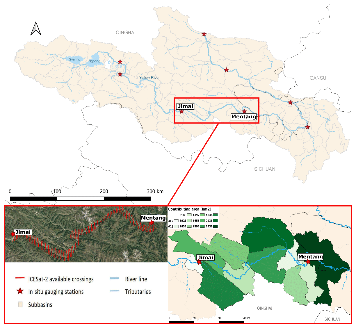
Figure 1 Area of interest and in situ gauging stations in the upstream area of the Yellow River. Calibration is performed for the river reach between Jimai and Mentang (red box and magnified inset). The bottom right image represents the catchment area along the river reach. The bottom left image shows the ICESat-2 crossings available in the river stretch.

3 Data

3.1 ICESat-2

ICESat-2 is an altimetry mission that has been operating since November 2018. This mission has 1387 reference ground tracks (RGTs) that are measured every 91 d. Each RGTs contains three pairs of ground tracks, and each pair is formed by a strong beam and a weak beam. The strong and weak beams have transmitted energy of 175 and 45 µJ per pulse, respectively (Neumann et al., 2021). The strong–weak beam pair is separated by 90 m, and each pair of beams is separated by 3.3 km. With this configuration, ICESat-2 provides a wide inter-track spatial coverage, covering large areas with altimetric measurements.

ICESat-2 data are acquired from the National Snow and Ice Data Center (NSIDC) portal and the National Space Institute at the Technical University of Denmark (DTU Space) database for the period between 31 October 2018 and 2 April 2021. Two different product levels are used, namely ATL03, with ATLAS/ICESat-2 L2A Global Geolocated Photon Data, and ATL13, with ATLAS/ICESat-2 L3A Along Track Inland Surface Water Data, which both have a temporal resolution of 91 d.

The pulse repetition frequency of ATLAS (Advanced Topographic Laser Altimeter System) corresponds to an along-track resolution of 70 cm. Depending on the number of photons that return to ATLAS, the ATL03 product can offer an along-track resolution down to 0.7 m and provides the geolocated photon event downlinked from ATLAS. The signal photon events are distinguished from the background events by calculating the signal-to-noise ratio. We use this product to map the land topography of the river cross section and measure hydraulic parameters such as river flow width and WSE, as explained in Sect. 4.1.1.

The ATL13 product provides inland WSE with an ensemble error of 6.1 cm per 100 inland water photons (Jasinski et al., 2021a). The along-track resolution of this product varies but is typically of the order of a few meters. We use this product to extract mean WSE at river crossings for the steady-state model calibration. The ATL13 data are prepared for the period between 31 October 2018 and 21 September 2020. In addition, there is a validation dataset in the period from 13 December 2020 to 19 October 2021. The periods for the calibration and validation datasets are defined according to the in situ discharge observations available at Jimai and Mentang gauging stations (see Sect. 3.2).

3.2 In situ data

In situ observations from Jimai and Mentang gauging stations were kindly provided by the Yellow River Conservancy Commission (YRCC). The available data cover the period between 10 May 2018 and 21 September 2020. Discharge data at both stations are used as boundary conditions for the steady-state hydraulic model that simulates WSE along the river reach from the given discharge. Jimai station provides data for both the low-flow and high-flow seasons, while Mentang station is missing the data for the low-flow season. Data from the period between 13 December 2020 and 19 October 2021 are available to validate the model.

3.3 Ancillary datasets

A 3 arcsec digital elevation model (DEM), flow accumulation map, and flow direction map are downloaded from the MERIT global database (Yamazaki et al., 2019). A conceptual river basin model is developed in which the major runoff generating catchments are identified at the main tributaries of the river reach. TauDEM (Terrain Analysis Using Digital Elevation Models) is used to delineate the river network and catchments with the information extracted from the MERIT database (Yamazaki et al., 2019). The river delineation is used as reference for the river centerline when defining river cross sections. The chainage of the river is generated from the river delineation with steps of 10 m, which is referenced to Ngoring Lake, close to the river source in the Bayan Har Mountains. The water occurrence map is downloaded from the Global Surface Water Explorer (Pekel et al., 2016). The water occurrence is used to filter the WSE observations from ATL13.

4 Methods

An overview of the workflow, including different data processing and modeling steps, is presented in Fig. 2. The method uses two different ICESat-2 data products as input and a steady-state 1D hydraulic model in the inverse hydraulic parameter calibration process. The ATL03 and ATL13 products are processed (see Sect. 4.1.1 and 4.1.3) to be ingested together with in situ discharge data in a hydraulic model calibration to estimate river flow depth, roughness coefficient, and riverbed shape. The calibrated model is used to calculate rating curves relating discharge and WSE and to interpolate the WSE time series along the river stretch. In addition, the parameter values are used to run a full 1D hydrodynamic simulation.

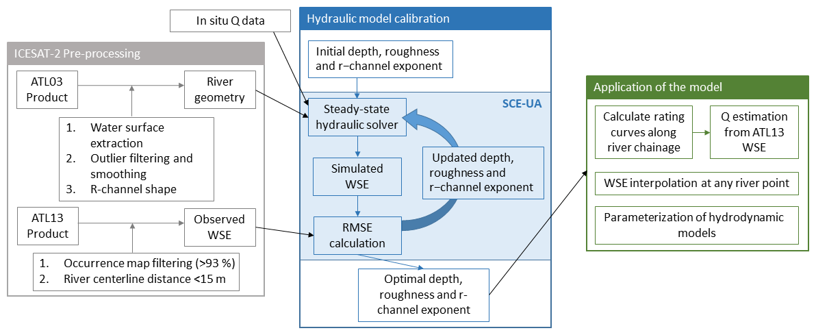
Figure 2 Schematic diagram of the data processing and modeling workflow in this study. The methodology proposes a series of applications from a calibrated model.

4.1 ICESat-2 land and WSE data processing

4.1.1 ATL03 cross section processing

The ATL03 photon cloud product is used to define riverbed geometry. To ensure that as large a portion of the riverbed as possible can be extracted from ICESat-2 observations, only the low-flow season crossings are taken into account, corresponding to the period between November and April. In addition, to select good quality cross sections, a visual inspection is also performed. The strong beam and weak beam data, separated by 90 m, were observed to behave differently, depending on the acquisition date. For the cases in which the strong beam signal was very strong, the data can present noise that complicates the processing steps, so the weak beam crossing is selected. For acquisitions with weaker signals, the topography is better mapped by the strong beam signal.

The water surface in the ATL03 data is characterized by a dense cloud of photons. A Gaussian kernel distribution is used to identify the water surface by taking the peak density value of the distribution. The points between 20 cm from the peak value are also identified as water surface and averaged. The river width is computed as the along-track extent of the water surface, taking into account the crossing angle between ICESat-2 ground track and river centerline.

To remove outliers from the photon cloud, two different methods are used. First, a Hampel filter is applied, in which the median absolute deviation (MAD) is computed for a sliding window in a 3.5 m ground track interval. A value will be considered an outlier if it exceeds the MAD. The MAD is defined as in Eq. (1):

$$\begin{array}{}\text{(1)}& \mathrm{MAD}=\mathrm{median}\left(\mathrm{|}{X}_i-\stackrel{\mathrm{̃}}{X}\mathrm{|}\right),\end{array}$$

with $\stackrel{\mathrm{̃}}{X}=\mathrm{median}\left(X\right)$. After the Hampel filter, a median filter is applied for the same 3.5 m ground track intervals. The ground track interval is a “window” that slides, entry by entry, and replaces each entry value with the median of the neighboring entries. Finally, in order to obtain a well-defined shape of the river cross section, a simple moving average (SMA) is computed for ground track intervals of 3.5 m.

4.1.2 R shape geometry for submerged portion

In the submerged portion of the channel, the ATL03 product does not detect the riverbed elevation. ATL03 product can successfully map bathymetry for clear waters, as shown by Parrish et al. (2019), who present results mapping the seafloor bathymetry. The portion of the area upstream of the Yellow River that we focus on (see Sect. 2) is characterized by fast and turbulent flow, which explains why bathymetry cannot be detected by ICESat-2 in this area. To cope with this limitation, the riverbed elevation in the submerged portion of the river is extrapolated using the approach proposed by Dingman (2007), which has been previously used for discharge estimates in Bjerklie et al. (2018). The shape of the submerged portion depends on a cross section form exponent r, with r=1 corresponding to a triangle and r→∞ corresponding to rectangular shape. The height above the lowest channel elevation, z, is approximated by Eq. (2), as follows:

$$\begin{array}{}\text{(2)}& z=Y_m^{*}{\left({\displaystyle \frac{\mathrm{2}}{W^{*}}}\right)}^r{x}^r,\mathrm{0}\le x\le W^{*}/\mathrm{2},\end{array}$$

where $Y_m^{*}$ is the low-flow depth, W^* is the bank width, and x is the horizontal distance from the river centerline. Figure 3 shows the different processing steps applied to ATL03 data to define the riverbed geometry. In the last step, the submerged portion is interpolated; thus, for each cross section, there are two free parameters ($Y_m^{*}$ and r) that will be estimated in the hydraulic inversion (see Sect. 4.3).

Figure 3 ATL03 photon cloud where the water surface is identified (a). The outliers are removed using Hampel and median filters (b). Smoothing of the cross section with SMA (c). Interpolation of the submerged portion (d).

4.1.3 ATL13 data processing

The model calibration needs an adequate selection of WSE data from ATL13 or other suitable altimetry missions. Radar altimetry missions, such as CryoSat-2 or Sentinel-3 cannot provide high-accuracy measurements in this area due to their low spatial resolution (250–300 m). The river stretch we focus on has a river width varying between 80 m in the low-flow season and a few hundred meters in the high-flow season. The ATL13 product offers a variable resolution depending on the acquisition date, but it is normally of the order of few meters (Jasinski et al., 2021a). This ICESat-2 product offers a variety of data quality flags to discard invalid measurements. In Xu et al. (2021), the following flags are considered for WSE assessments: qf_bckgrd, qf_bias_em, qf_bias_fit, stdev_water_surf, and snow_ice. These flags control the density of background photons, electromagnetic bias and bias in the fit, standard deviation of WSE, and presence of snow or ice. After applying the flags, Xu et al. (2021) recommend an extended outlier filtering method. Moreover, the ATL13 data product presents known issues, such as including land area adjacent to WSE or land measurements in the low-flow season, that need to be considered (Jasinski et al., 2021b).

The morphological characteristics of the river make the selection of good WSE observations challenging. The river stretch presents braided structures in selected areas in which the ATL13 product can mix the land in between channels with water surface. To avoid this issue, we first apply the water occurrence map from Global Surface Water Explorer (Pekel et al., 2016), only including observations that fall over pixels with water occurrence larger than 93 %, a threshold that is exceeded in very few pixels. Taking into account the river delineation extracted from the MERIT database (Yamazaki et al., 2019; see Sect. 3.3), we only consider WSE points that are less than 15 m away from the river centerline, to ensure that ATL13 observations fall in the water surface in the low-flow period, when we have flow widths around 80 m for selected areas. The points that are within 15 m from the river centerline are averaged to have a unique observation for different dates at every chainage point. In addition, all the WSE measurements within the same acquisition date that are less than 500 m away from each other, and where the WSE variation is less than 15 times the slope times the distance between observations, are averaged. This last criterion is taking into account the computational grid resolution of the hydraulic model, which is 300 m and refined to 100 m in selected areas (see Sect. 4.2).

We compared the performance of the filtering process with the quality flags, taking the values proposed by Xu et al. (2021), qf_bckgrd < 6, |qf_bias_em| < 2, |qf_bias_fit| < 2, and constraining the water surface standard deviation, stdev_water_surf to 0.5 m. The snow_ice flag was also applied but with no presence of ice for the area of interest. The results are better when we filter with respect to the river centerline and water occurrence map than when using the ATL13 quality flags. After applying the quality flags only, some of the points that fall on the adjacent land area are not removed.

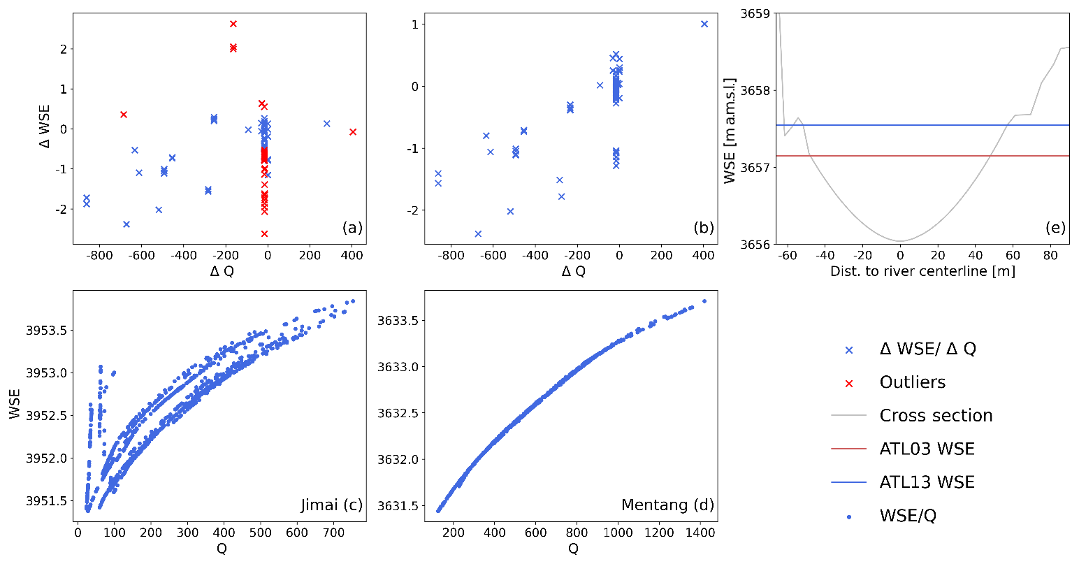
Figure 4 Variation in discharge against WSE from ATL03 and ATL13 (a). Variation in discharge against the variation in WSE from ATL03 and ATL13 after correction (b). Rating curve (discharge against WSE) for the Jimai gauging station (c). Rating curve for the Mentang gauging station (d). Example of mismatch between ATL13 and ATL03 WSE (e).

4.1.4 Cross sections and observation points selection

Cross-sectional data from ATL03 are selected for the available dates in the low-flow season. Depending on the acquisition dates, the discharge varies and, accordingly, the reference WSE of the cross section changes. This can lead to unreasonable variations in the bottom elevation when constant depth is assumed, thus leading to simulation errors. To avoid such errors and have a realistic reference bottom level (BL), we define a reference WSE. The reference WSE is taken from the ATL03 cross section in which the acquisition date has the lowest discharge value from the in situ data. The discharge variation is calculated between the lowest in situ discharge value and the in situ discharge values for ATL03 cross section acquisition dates. Since the discharge variation should be proportional to the WSE variation, we define a correction factor α relating the discharge variation to the WSE variation as $\mathrm{\Delta }\mathrm{WSE}=\mathit{\alpha }\cdot \mathrm{\Delta }Q$. The correction factor α is a calibration parameter, and we add α⋅ΔQ to the corresponding cross section depth value.

To confirm that the discharge variation and the WSE between ATL03 and ATL13 are consistent, we compare the WSE measured by the ATL03 and the ATL13 for the values that are closer than 300 m, according to the resolution of our model, and the variation in discharge between the ATL03 and ATL13 acquisition dates. The analysis can be seen in Fig. 4a. The method we use to detect the WSE in the ATL03 product is different from the one used to produce the ATL13 product (see Sect. 4.1.1); hence, we can find differences between our detected WSE and the one provided by ATL13 product for the same acquisition data. An example of the difference between WSE detected in ATL03 and ATL13 WSE can be seen in Fig. 4e, where there is an offset between elevations of about 0.41 m. This would explain some of the points that lie close to ΔQ=0, for which ΔWSE is different from 0, in Fig. 4a. To avoid this problem, we substitute the WSE at each ATL03 cross section by the value given in the ATL13 product, and the submerged portion is interpolated based to this value. By substituting these values, some of the discharge variations that were not in accordance with the WSE variation were corrected; for example, the value lying close to ΔWSE=0 and ΔQ=400 in Fig. 4a lies closer to ΔWSE=1 in Fig. 4b.

In addition, the Jimai rating curve presents some anomalies (Fig. 4c) in which the discharge–WSE pair does not follow the power law (points with low discharge values have a high WSE value) that could be explained by the freezing of the water surface in the station area. We observed that the outliers in Fig. 4a were related to the rating curve anomalies (ΔWSE around 2 m and ΔQ close to −200 m³ s⁻¹), and the ATL03 and ATL13 data taken at the corresponding dates were rejected. After this analysis, the resulting relation between ΔQ and ΔWSE can be seen in Fig. 4b.

4.2 1D hydraulic model

The 1D hydraulic model is defined by assuming steady state. This assumption is reasonable for ATL13 observations after filtering and checking that the discharge varies consistently with WSE (see Sect. 4.1.3 and 4.1.4). The steady-state hydraulic solver is based on the Saint-Venant equations in the steady state. These equations express the mass and momentum balance in an open channel, as given by Eq. (3).

$$\begin{array}{}\text{(3)}& \begin{array}{rl}q& ={\displaystyle \frac{\partial A}{\partial Q}}+{\displaystyle \frac{\partial Q}{\partial x}},{\displaystyle \frac{\partial Q}{\partial t}}+{\displaystyle \frac{\partial }{\partial x}}\left({\displaystyle \frac{\mathit{\beta }{Q}^{\mathrm{2}}}{A}}\right)\\ & +gA{\displaystyle \frac{\partial h}{\partial x}}-gA\left(S_{\mathrm{0}}-S_{\mathrm{f}}\right)=\mathrm{0}\end{array}\end{array}$$

The steady-state assumption implies constant discharge over time; hence, all time derivatives are zero. The x is the chainage or distance along the channel, h is channel depth, A is the flow cross-sectional area, q is the lateral inflow, Q is the discharge, S₀ and S_f are the bed and friction slopes, respectively, g is the gravitational constant, and β is the momentum coefficient which is set to 1.

From the steady-state solver, we calculate WSE profiles from a given discharge and water level at the downstream point, as described in Kittel et al. (2021). The WSE is computed step-wise at Δx spatial increments and moves upstream along the channel. The equation to solve this is presented in Eq. (4), which is based on the steady-state Saint-Venant equations, assuming subcritical fluvial flows, and where the right-hand side (RHS) is the collection of terms not containing the derivative of the depth with respect to the chainage (see Kittel et al., 2021, for the full derivation). The K in Eq. (4) refers to conveyance.

$$\begin{array}{}\text{(4)}& \mathrm{RHS}(x,h(x\left)\right)={\displaystyle \frac{\left(\frac{Q^{\mathrm{2}}}{g{A}^{\mathrm{3}}}\frac{\partial A}{\partial x}+S_{\mathrm{0}}-\frac{Q^{\mathrm{2}}}{K^{\mathrm{2}}}-\frac{\mathrm{2}Qq}{g{A}^{\mathrm{2}}}\right)}{\mathrm{1}-\frac{Q^{\mathrm{2}}}{g{A}^{\mathrm{3}}}\frac{\partial A}{\partial x}}}\end{array}$$

The model is initialized by calculating the downstream WSE from the in situ discharge, assuming uniform flow and using Manning's equation and the local slope bed value between the two most downstream cross sections. This value is initialized at 0.0011 m km⁻¹ and updated at each iteration. Equation (4) is solved explicitly, as expressed in Eq. (5):

$$\begin{array}{}\text{(5)}& h_{i-\mathrm{1}}=h_i-\mathrm{RHS}\left(x_i,h_i\right)\cdot \mathrm{\Delta }x.\end{array}$$

The chainage grid is defined with step increments of 300 m in between observed cross sections, when the slope is less than 0.20 m km⁻¹, for the sections of the river reach with steeper slope (≥0.20 m km⁻¹) or, for areas in which the neighboring cross sections present a significant difference in low-flow width, the step increment is reduced to 100 m to avoid instability of the explicit numerical scheme. To make sure that the model results are independent of the chosen grid discretization, different forward runs were made for step size down to 50 m, and differences in the simulated WSE were shown to be insignificant.

4.2.1 Boundary conditions

The downstream boundary is defined as a free, uniform outflow boundary condition (Li et al., 2017). This boundary is defined 10 km away from the downstream station by duplicating the ATL03 cross section defined closest to the Mentang station. To initialize the steady-state solver, a value of WSE at the downstream point is calculated from in situ discharge values, using Manning's equation.

The lateral inflow q is distributed along the chainage proportionally to the contributing area (see Fig. 1), taking into account the discharge variations from upstream and downstream in situ data. The lateral inflow at chainage x is computed as in Eq. (6).

$$\begin{array}{}\text{(6)}& q={\displaystyle \frac{Q_x-Q_{x-\mathrm{1}}}{\mathrm{\Delta }x}}\end{array}$$

To calculate the discharge at chainage x, Q_x, we assume that the runoff in the catchment is uniformly distributed, i.e., boundary inflow is proportional to the increment in contributing area, as defined by the term upstream drainage area (UPA), which is available in the MERIT dataset (see Sect. 3.3). Instead of calculating a rainfall–runoff model, we use in situ discharge measurements at two available stations Jimai (upstream discharge Q_up) and Mentang (downstream discharge Q_down; see Sect. 2). For the downstream station, Mentang, the available data are between May and November, while for the upstream station, Jimai, data are available for the whole period. Hence, two possible scenarios are taken into account.

1. If in situ observations are available at both upstream and downstream stations, then the distributed discharge at chainage point x is as in Eq. (7).

   $$\begin{array}{}\text{(7)}& Q_x=Q_{\mathrm{up}}+{\displaystyle \frac{{\mathrm{UPA}}_x-{\mathrm{UPA}}_{\mathrm{up}}}{{\mathrm{UPA}}_{\mathrm{ds}}-{\mathrm{UPA}}_{\mathrm{up}}}}\left(Q_{\mathrm{ds}}-Q_{\mathrm{up}}\right)\end{array}$$

2. If only upstream in situ data are available, which is the case for the low-season period (October to May), then we consider the discharge at chainage point x to be as in Eq. (8).

   $$\begin{array}{}\text{(8)}& Q_x=Q_{\mathrm{up}}+{\displaystyle \frac{{\mathrm{UPA}}_x-{\mathrm{UPA}}_{\mathrm{up}}}{{\mathrm{UPA}}_{\mathrm{up}}}}\left(Q_{\mathrm{up}}\right)\end{array}$$

4.3 Parameter estimation

The objective of the parameter estimation is the retrieval of riverbed geometry characteristics, i.e., $Y_m^{*}$ and r (Eq. 2) in addition to Manning's roughness for each cross section. To estimate the hydraulic parameters, model calibration is performed for four spatially uniform parameters, i.e., low-flow depth, Manning's roughness, the r shape exponent, and a correction factor α. The calibration algorithm we use is the Shuffled Complex Evolution method from the University of Arizona (SCE-UA), as presented by Duan et al. (1992) and implemented in Python using SPOTPY (Houska et al., 2015). The SCE-UA is a global optimization algorithm that samples the parameter space using complexes. Each complex is evolved independently according to the competitive complex evolution (CCE), presented by Nelder and Mead (1965), and shuffled (re-partitioned) after each evolution to ensure an efficient global search. For the method to give a better overall performance, the number of complexes is set to 2n+1, where n is the number of parameters (Duan et al., 1993). In our optimization algorithm, we work with nine complexes. The objective function is the standard deviation of the prediction error between the ATL13 WSE and the simulated WSE, which is known as the root mean square error (RMSE).

$$\begin{array}{}\text{(9)}& \mathrm{Obj}=\sqrt{{\displaystyle \frac{\mathrm{1}}{N}}\sum _{i=\mathrm{1}}^N{\left({\mathrm{WSE}}_{\mathrm{sim}}-{\mathrm{WSE}}_{\mathrm{ATL}\mathrm{13}}\right)}^{\mathrm{2}}}\end{array}$$

The low-flow depth varies between 1.3 and 2.5 m, and its initial value is 2 m. The Manning roughness varies between 0.027 and 0.06 s m${}^{-\mathrm{1}/\mathrm{3}}$, and it is initialized at 0.031 s m${}^{-\mathrm{1}/\mathrm{3}}$. The r shape exponent varies between 1 and 3, and it is initialized at 1.8. The correction factor α varies between 0.0005 and 0.003 m m⁻³ s, and it is initialized at 0.002 m m⁻³ s. For the parameter prior distribution, we choose a uniform distribution. The sensitivity of the parameters in the model calibration is computed using Fourier amplitude sensitive test (FAST), as proposed by Saltelli et al. (1999).

4.4 Lateral inflow analysis

To produce good estimates of WSE and discharge from a 1D hydraulic model, the inference of adequate parameters and definition of boundary conditions is fundamental. The main source of uncertainty in the model comes from the lateral inflow (for which measurements are not available). The lateral inflow boundary is defined using the MERIT flow accumulation map, as explained in Sect. 4.2.1. To study the sensitivity of the model to the lateral inflow definition, we also run a calibration that assumes a uniform lateral inflow along the simulated chainage interval. Since the MERIT flow accumulation accounts for the tributary contributions, we expect that the model performance will degrade when uniform lateral inflow is assumed instead of uniform runoff.

4.5 Application and use cases

4.5.1 WSE densification and discharge retrieval

The calibrated model reproduces WSE–discharge relationships in the form of rating curves. We produce a series of rating curves along the river stretch for a given downstream discharge value to create a lookup table between river chainage, WSE, and discharge. This relation can be used for different applications.

1. Densification of WSE. This is the aim of several studies that use different methods to interpolate altimetry WSEs, i.e., by using Kriging methods (Boergens et al., 2017; Yoon et al., 2013) or by interpolation using WSE (Villadsen et al., 2015). In our case, we use the calibrated 1D hydraulic model to calculate WSE along the river stretch. Using ATL13 observations at different acquisition times, we can predict WSE at any river point using the calibrated model.

2. Discharge retrieval. The calibrated model can be used to convert ATL13 WSE observations into estimates of river discharge using WSE–discharge relations (Malou et al., 2021). At any time of ICESat-2 acquisitions, or any other type of altimetry data, we can ingest an observation of WSE to produce discharge estimates for any point of the river stretch using the estimated rating curves from the 1D hydraulic model.

4.5.2 Parameterization of hydrodynamic (HD) models

The optimal parameters from the 1D hydraulic calibration can subsequently be transferred to a full hydrodynamic model simulation if predictions of dynamics of discharge and WSE are of interest. To demonstrate the ability of the method in the parameterization of full hydrodynamic simulations in the transient state, we use MIKE HYDRO River (Havnø et al., 1995). This is a 1D hydrodynamic model that uses a dynamic wave solver of the 1D Saint-Venant equations. To run the hydrodynamic model, we use daily in situ discharge data as an upstream boundary for a period of 3 years. MIKE HYDRO River uses the calibrated cross sections to obtain information on calibrated channel geometry and optimal Manning's roughness coefficient. The runoff increments are distributed according to the contributing area, which is obtained from the MERIT flow accumulation map.

5 Results

5.1 ICESat-2 data processing

5.1.1 ATL03 cross section processing and selection

The cross sections are visually inspected to identify if the land and water topography are well defined, and there are no signs of cloud formation or weather effects. In total, 80 ATL03 cross sections are selected which define the riverbed geometry along the river reach between Jimai and Mentang (see Fig. 5, bottom), including measurements of land elevation of the dry portion of the riverbed. Measurements are provided every 3.5 to 20 m. Closely spaced cross sections are removed to reduce the computational cost of the model, since only cross sections whose chainage differ by more than 500 m provide meaningful information due to the resolution of the 1D hydraulic model. In areas with scarce ICESat-2 data, there can be a separation between cross sections of up to 10 km. The gaps in the data at the scale of our investigation are mostly due to the poor quality of acquisitions in the period in which weather conditions are having an impact on the ICESat-2 observations. For the river stretches with little cross section information, we interpolate cross section in between using the MIKE HYDRO River cross section module; however, model performance is expected to be worse here.

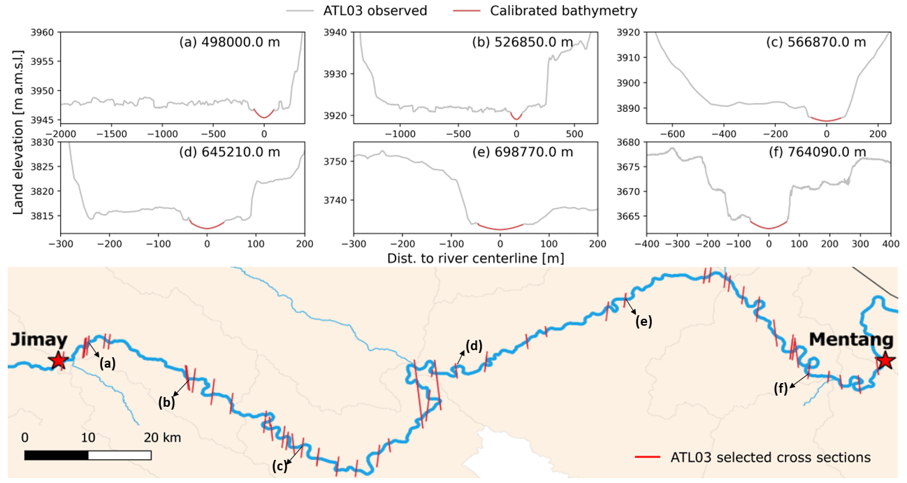
Figure 5 Panels (a–f) show examples of cross section geometry after calibration, where the majority of points correspond to ATL03 observed data. The bottom panel shows ATL03-selected cross sections for river hydraulic calibration. A total of 80 cross section were selected after the processing described in Sect. 2.1.1. The cross section shown in the top plot is located in the river.

The top panels of Fig. 5 give examples of the cross section geometry measured with ATL03 together with submerged portion that is not observable and has been calibrated. These cross sections give quite a reasonable representation of the river geometry. An advantage of the method is that most of the cross section points are from observed data, since the data are selected for the low-flow season. This gives a more accurate representation of the hydraulic geometry. In Fig. 5a and b, which correspond to the most upstream part, we can observe the presence of floodplains, with a braided structure of few kilometers, while the rest of the stretch has a confined structure.

5.1.2 ATL13 WSE processing

Initially, we use observations from 236 ATL13 data products, providing measurements in low-flow and high-flow seasons. The 236 ATL13 products contain 3199 WSE points, as illustrated by red crosses in Fig. 6. The ATL13 quality flags described in Sect. 4.1.3 are applied to the data after removing the largest outliers. The data, after applying the quality flags, are represented by light blue dots in Fig. 6. After applying the extra filtering methods, as explained in Sect. 4.1.3, we obtain 81 WSE observations. These observations cover the calibration period, between November 2018 and September 2020, and are illustrated in Fig. 6 by the blue circles. The processing steps provide a good sample of WSE observations, with good spatial coverage of the entire river reach. Moreover, the temporal coverage of the dataset includes low-flow and high-flow season observations, with a slight predominance in the low-flow season, which is related to the quality of ICESat-2 data for the different seasons. The filtering criteria are not biased against high-flow season observations.

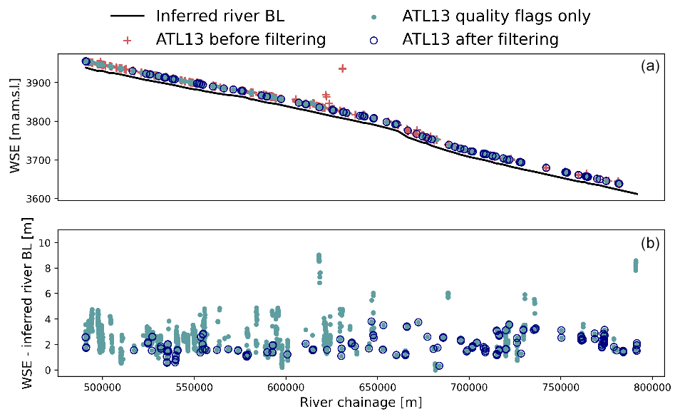
Figure 6 (a) ATL13 WSE along-river chainage before processing, after quality filters are applied, and after filtering criteria. (b) ATL13 WSE minus inferred BL from the model calibration is determined by comparing the quality filters results and the filtering criteria.

5.2 Calibration using ICESat-2 observations

To test the sensitivity of the model to the lateral inflow representation, we run two different calibrations. The first one assumes a uniform runoff distribution and a distribution of boundary inflow according to the MERIT flow accumulation map, and the second one assumes a uniform boundary inflow. Both calibrations are performed against ATL13 WSE observations for four spatially uniform parameters, namely low-flow depth, Manning's roughness, correction factor α, and cross section form exponent r. A forward run of the model takes 39 s, and the hydraulic model calibration converges after about 1000 runs. To speed up the calibration, we define discharge classes in which we group the WSE by the corresponding discharge value in the acquisition date. Acquisition dates with the same discharge value belong to the same class. In this way, each iteration includes individual runs for 29 different discharge classes. The minimum RMSE value of the calibration is taken as the optimal value, and results can be seen in Table 1. The RMSE is slightly better when using the MERIT flow accumulation map than when using uniform boundary inflow (0.41 and 0.42 m, respectively), which overall is in good agreement with previous studies (Jiang et al., 2019; Kittel et al., 2021a), considering the low parameterization of the model which considers uniform depth and roughness. The most sensitive parameters in the FAST sensitivity analysis are Manning's roughness and low-flow depth. Both calibrations improve the RMSE relative to the prior guess, which corresponds to 0.619 m. If we check the parameter space using the MERIT flow accumulation calibration, then the optimal parameter estimates (red diamond in Fig. 7) are not close to the a priori interval boundaries, which indicates that the parameter constraint was well defined. The most correlated parameters are roughness and depth, as seen in Fig. 7.

Table 1 Steady-state solver calibration results for uniform calibration values along the river stretch. The root mean square error (RMSE) is minimized. Uncertainty and sensitivity values correspond to the MERIT flow accumulation model. The sensitivity analysis is performed with FAST, and the values represent the ratio between the percent RMSE change and the percent of the parameter change. The uncertainty in the parameters is computed with the DiffeRential Evolution Adaptive Metropolis (DREAM) algorithm.

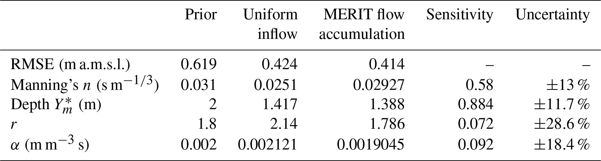
Figure 7 Sampling pattern and model performance during calibration using the MERIT flow accumulation map. The objective function is lowered during calibration.

To study the uncertainty in the model, we use a Bayesian uncertainty analysis, the DiffeRential Evolution Adaptive Metropolis (DREAM) algorithm, proposed by Vrugt (2016). We run the uncertainty analysis using the MERIT flow accumulation case, which is our best inference result. This algorithm creates a posterior sampling in the parameter space, from which we take the 10 % best model runs to create the posterior distribution. Figure 8 compares the simulated WSE minus the inferred bottom level (BL), using the MERIT flow accumulation, and the ATL13 WSE minus inferred BL. Overall, the simulated WSE corresponds to the ATL13 WSE with a deviation below 1 m (Fig. 8a). The larger errors are found for selected observations in the downstream area and for observations between chainage 650 000 and 680 000 m (Fig. 8b).

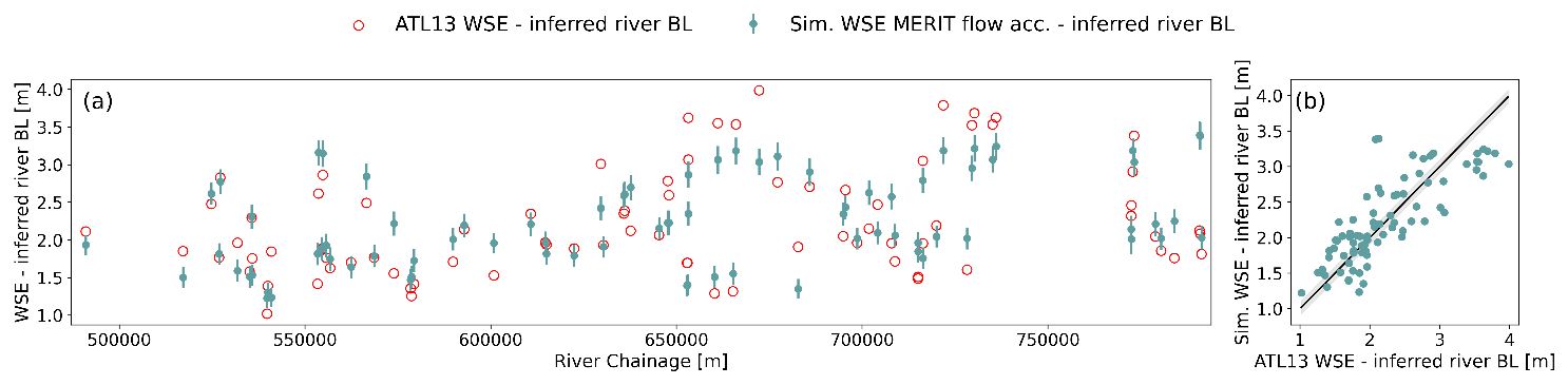
Figure 8 (a) Calibrated longitudinal profile using the steady-state solver for uniform depth and the MERIT flow accumulation between Jimai and Mentang. (b) Simulated vs. ATL13 WSE minus inferred BL. The shaded area corresponds to the mean standard deviation in the ATL13 product, as extracted from the flag stdev_water_surf.

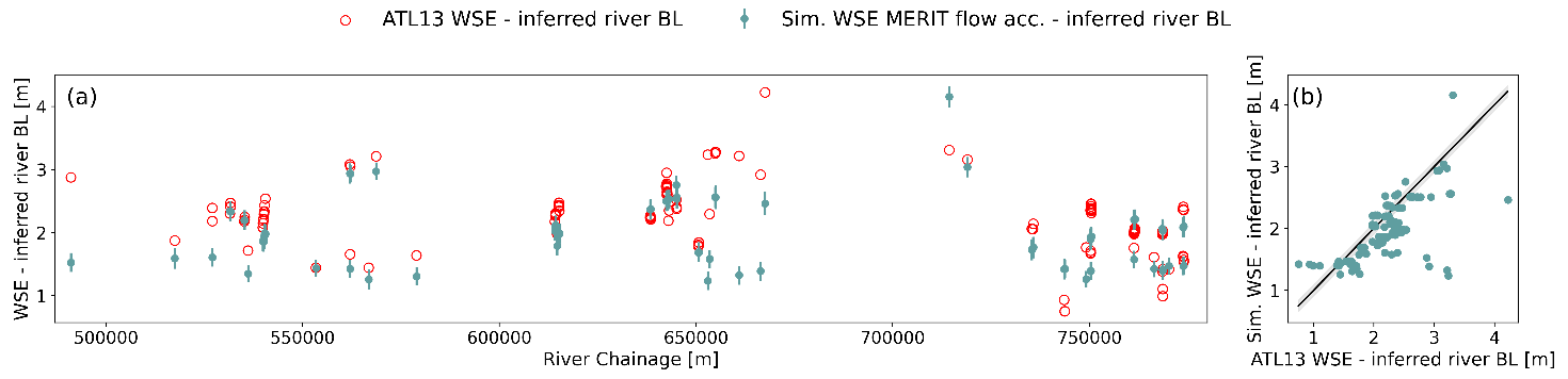
Figure 9 (a) Validation longitudinal profile using the steady-state solver for uniform depth and the MERIT flow accumulation between Jimai and Mentang. (b) Simulated vs. ATL13 WSE minus inferred BL. The shaded area corresponds to the mean standard deviation in the ATL13 product, as extracted from the flag stdev_water_surf.

5.2.1 Validation of the model calibration

The validation data consist of ATL13 observations for the period between 13 December 2020 and 19 October 2021 in which in situ discharge is used to force the hydraulic model in this period, assuming uniform runoff and boundary inflow distributed according to the MERIT flow accumulation map. In the validation period, the RMSE of the model is 44.3 cm, which is in good agreement with the calibration RMSE. The error in the validation data can be seen in Fig. 9. The deviation from the ATL13 WSE minus inferred BL goes up to 1.5 m (Fig. 9a). We observe again that a larger error is present between chainage 650 000 and 680 000 m (Fig. 9b), as previously seen in the calibration data.

5.2.2 Rating curves along the river stretch

The rating curves define the relation between WSE and discharge along the river reach. Rating curves depend on hydraulic characteristics of the channel, so an accurate parameterization is necessary. The WSE–discharge relation generally follows a power law. We calculate rating curves every 50 m from the calibrated hydraulic model. This defines a lookup table relating discharge, WSE, and river chainage. Examples of rating curves in the lookup table are illustrated in Fig. 10, where the flow depth, computed as simulated WSE minus calibrated BL, is compared to the discharge. The computed rating curves follow a power law. We can also see that, for the more upstream point at 491 020 m, the discharge values are lower than the ones further downstream.

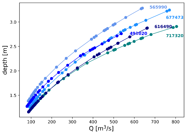
Figure 10 Examples of simulated rating curves relating WSE and discharge at different chainage points.

Note that, for the relation at chainage 565 990 m, the increase in flow depth is larger than for other examples. This effect is produced due to the narrower river width at this river location that produces an increase in flow depth for the same discharge values. This is a clear example of the river geometry effect in building WSE–discharge relationships.

5.2.3 Validation of rating relationships and demonstration of model applications

The results of the validation are presented as the percentage of flow exceedance for a given discharge value and are compared with in situ data (Fig. 11a and b). The estimated discharge values are for selected ATL13 WSE observations. The validation dataset, corresponding to the period from 13 December 2020 to 19 October 2021, is ingested together with the calibration data in the hydraulic model to interpolate the corresponding discharge at the time of acquisition at a given river location (Jimai and Mentang gauging stations). The estimation using the MERIT flow accumulation, uniform boundary inflow, and the prior guess is presented. The percentage of flow exceedance for the estimated discharge is in good agreement with the in situ data for the MERIT flow accumulation case. For Mentang station (Fig. 11b), the observed Q₆₀ is about 400 m³ s⁻¹, while the simulated Q₆₀ is around 250 m³ s⁻¹, which is a considerable difference. For the case using uniform inflow and the prior guess, the difference with in situ data is larger, mostly for the larger values of discharge, which is from 400 m³ s⁻¹ at Jimai and from 500 m³ s⁻¹ at Mentang. In the simulated discharge, we are also calculating low-flow values that are missing in the in situ measurements, which explains this mismatch.

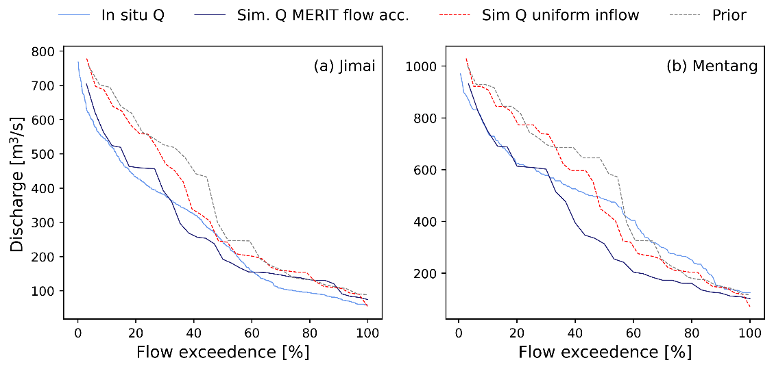
Figure 11 Simulated discharge vs. in situ measured discharge at Jimai (a) and Mentang (b) stations.

Table 2 presents the RMSE using the three different approaches. The best results with the lower RMSE are from using the MERIT flow accumulation with RMSE 107 m³ s⁻¹ at Jimai and 122.38 m³ s⁻¹ at Mentang. When using the uniform inflow, the difference in RMSE is not significant in Mentang (127.43 m³ s⁻¹), but it increases for Jimai discharge estimations (149.30 m³ s⁻¹). In the case of the prior guess, it is quite clear that the results are worse than for the calibrated models.

Table 2 RMSE between in situ discharges measured at Jimai and Mentang stations and the estimated discharge. Three different cases are presented, using the MERIT flow accumulation map, uniform inflow, and the estimations with the prior guess.

There are two different virtual stations (VSs) available from Hydroweb in this area of the Yellow River (Normandin et al., 2018) at kilometer 4914, corresponding to chainage 545 030 m, and at kilometer 4901, corresponding to chainage 560 360 m. We compare the Sentinel-3-derived Hydroweb VS time series at these two points, with the WSE estimated by the model using the MERIT flow accumulation map (Fig. 12). The only available ATL13 observation in this area is represented by the blue star in Fig. 12a, which falls very close to the ATL13-derived WSE time series. It is clear, in Fig. 12a, that the Sentinel-3-derived WSE is not well represented, probably due to the low resolution of this mission and the mountainous terrain, which reduce the accuracy of the retrieved WSE in this area. The seasonality is not present in the Hydroweb VS time series, and some low-flow season values are above the high-flow season values, which should not be the case. The offset with the observed and estimated WSE from ATL13, which is expected to perform better due to its resolution, is more than 2 m and mostly in the low-flow season. A general bias in the data of this VS can be also observed. In Fig. 12b, ATL13-derived values match slightly better with the WSE from the VSs; however, the VS time series present large uncertainties, and the seasonality is poorly represented.

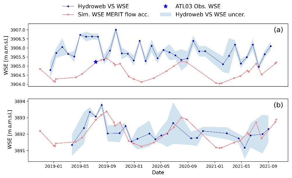
Figure 12 Comparison of estimated WSE with available Hydroweb VS in the area of interest (AOI). The WSE at VSs is derived from Sentinel-3A observations. (a) Simulated WSE at chainage 545 030 m vs. WSE at VS 4914 km. (b) Simulated WSE at chainage 560 360 m vs. WSE at VS 4901 km.

Figure 13 shows examples of WSE (Fig. 13a, c and e) and discharge (Fig. 13b, d)and e) time series for three different river locations at chainage 491 020, 565 990, and 717 320 m. The results are interpolated from ATL13 observations using the WSE–discharge relation at the selected river locations. In situ measurements for WSE to compare with the simulated values are not available. The figure shows the estimation using the MERIT flow accumulation and compares it with the estimation using the uniform inflow and the prior guess. The discharge estimated from the prior and uniform inflow are clearly overestimated compared with the MERIT flow accumulation case. This was also observed in Fig. 11 when we compared it with in situ discharge. The main difference between the prior and calibrated parameters can be seen in Fig. 13e at the more upstream example. The larger depth in the prior guess (2 m) is clearly making an impact in this area, since we expect to have a shallower depth upstream.

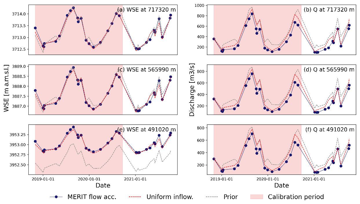
Figure 13 Simulated WSE (a, c, e) and simulated discharge (b, d, f) at selected chainage points. The simulated WSE and Q from the MERIT flow-accumulation-inferred parameters is compared with the results using uniform inflow and the prior guess.

5.2.4 Parameterization of HD model

The calibrated Manning's roughness together with the calibrated cross sections are used in MIKE HYDRO River to run a full hydrodynamic model simulation. The model runs in a grid with 1 006 558 grid points which consist of pairs with a timestamp for chainage. We define 2 min time steps and 100 m distance. We define a boundary condition at the upstream cross section with input discharge from Jimai in situ data and a downstream boundary at the synthetic cross section relating discharge and stage. We use the dynamic wave solver that corresponds to the full 1D Saint-Venant equations. Figure 14a compares the simulated WSE by MIKE HYDRO and ATL13 WSE minus inferred BL. MIKE simulations seem to be underestimated in most of the cases, and the maximum deviation from the ATL13 WSE minus inferred BL is around 1.7 m. The RMSE is 0.59, which is in good agreement with the results from the steady-state solver.

Figure 14b presents the WSE time series at chainage 491 020 m, as simulated from MIKE and from the steady-state solver. The time series represent the seasonal variation fairly well. The simulated values from the steady-state solver appear to be above the ones from MIKE simulation. This was also observed when we compare the simulated MIKE WSE with the observed ATL13 WSE minus the inferred BL (Fig. 14a), which makes sense if we take into account that the simulated water surface from the steady-state solver is directly derived from ATL13 observations, while the simulated MIKE WSE is derived from discharge observations.

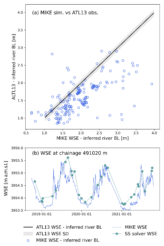
Figure 14 (a) MIKE HYDRO simulated WSE vs. ATL13 WSE minus inferred BL. The shaded area corresponds to the median SD (standard deviation) of the ATL13 observations, as taken from the flag stdev_water_surf. (b) Simulated WSE from the steady-state solver and MIKE.

6 Discussion

6.1 ICESat-2 data selection

ICESat-2 data provide valuable information for river hydraulic modeling. The ATL03 product gives accurate river geometry measurements. The low-flow river width could be retrieved from this product together with measurements of the river dry portion. This is an advantage with respect to other studies in which satellite altimetry could only be used in wider river channels (Lettenmaier et al., 2015; Kittel et al., 2021a; Jiang et al., 2019). The processing of the ATL03 photon cloud dataset provides a well-defined shape of the river cross section for the non-submerged portion, removing background noise and outliers. Previous studies on hydraulic calibration used hydraulic signatures from satellite remote sensing measurements, but they did not include observations of cross section geometry. Instead, they use simplified geometries (Bjerklie et al., 2018; Pujol et al., 2020; Garambois et al., 2020).

The method works best in west–east oriented rivers, where the density of ICESat-2 tracks that are almost perpendicular to the river centerline is highest. However, thanks to the densely spaced ICESat-2 tracks, with an inner track spacing of less than 2 km (Markus et al., 2017), this method can also be used in rivers with dominant south–north orientation because natural rivers will always include curved reaches where the orientation of the river changes or where the cross sections can be corrected and re-projected.

Accurate WSE observations are very important in the calibration process. The ATL13 product gives a well-distributed sample in both the space and time of WSE data. However, several outliers are present, which need a closer look. Besides the quality flags that the product provides, an outlier filtering process was defined based on the water occurrence and river centerline. Applying these two criteria, the main outliers were successfully removed without rejecting good quality observations.

The main drawback of ICESat-2 data is the inability to operate in all weather conditions, since the laser altimeter cannot penetrate thick clouds. This creates gaps in the cross-sectional data of up to 10 km. However, future acquisitions on the corresponding ground tracks can be used to fill these gaps.

6.2 Model performance

We presented a spatially uniform flow depth and roughness calibration against ATL13 WSE. The steady-state assumption and low parameterization, with only four calibration parameters, makes the model converge fast due to using a global search algorithm. Two different calibrations were compared to check the model sensitivity to lateral inflows, with one using the MERIT flow accumulation map and one assuming uniform inflow. The best calibration resulted from the MERIT flow accumulation case with a RMSE value of 0.41 m. This result was quite satisfactory with respect to other studies which used distributed depth calibration and applied it to wider river channels. Indeed, Jiang et al. (2019) obtained a RMSE between 0.72 and 1.6 m by using a combination of altimetry datasets over the Songhua River. Kittel et al. (2021b) present RMSE between 0.61 and 0.89 m using CryoSat-2 observations only on the Zambezi catchment. Pujol et al. (2020) use Envisat observations and synthetic SWOT to infer channel geometries, resulting in WSE RMSEs around 0.94 m. When using a multi-mission approach, Domeneghetti et al. (2021) report RMSEs between 0.68 and 0.89 m in the Po River. The parameters most sensitive to the calibration were the roughness coefficient and the low-flow depth, while the cross section form exponent and correction factor had a lower impact. The value of the cross section form exponent is most uncertain; however, changes in this value do not introduce large changes in the model. In addition to the uniform depth calibration, we attempted to calibrate distributed depth models, which did not improve the RMSE. The test was made for 5 and 10 uniformly distributed depths along the river reach with uniform Manning's roughness. Defining more parameters in the model increases the computational cost significantly, and convergence could not be reached in some cases. We observed a larger error between simulated and observed depth between chainage 650 000 and 680 000 m that was not removed when calibrating distributed depths. The WSE in this area seems to be underestimated for high-flow observations and overestimated for low-flow observations.

A validation dataset for a 10-month period is used in which the RMSE is 0.44 m and in good agreement with the calibration data. The same larger errors were observed between chainage 650 000 and 680 000 m.

In addition, we ran calibrations using 8 and 16 distributed Manning's roughness, where the RMSE improves to 0.377 and 0.365 m, respectively. However, when evaluating the validation data, the RMSE for 8 and 16 distributed roughness is 0.445 and 0.425 m, respectively (see Appendix A). The first case is an indicator of overfitting in the model. Increasing the distributed roughness coefficient to 16 reduces the RMSE by a few centimeters, but the computational cost of the calibration increases significantly.

Overall, the model performance is satisfactory compared to previous studies, with the added value of being a low parameterized model. In addition, the steady-state assumption significantly reduces the simulation time, which took 1:15 h for a period of 3 years in a full 1D hydrodynamic simulation, compared with the 39 s of steady-state forward run for all the discharge classes. These two factors make the convergence of the calibration process quite fast.

6.3 WSE densification and discharge estimation

ICESat-2 altimetry provides accurate elevation measurements at low temporal resolution. To create WSE and discharge time series, the interpolation of WSE is needed. We use the calibrated hydraulic model to create WSE–discharge relationships in the form of rating curves along the river stretch, an approach that has been previously used in other studies successfully (Malou et al., 2021). Rating curves make possible the interpolation of WSE and estimation of discharge at any point in the river for a given ATL13 WSE observation.

In Fig. 11, we compare the estimated discharge with the available in situ discharge at Jimai and Mentang stations in percent of flow exceedance. The estimations are reasonably good when we use the MERIT flow accumulation. Simplifying the model to the uniform boundary inflow accentuates the error at the upstream end, which shows the importance of defining the prior inflows accurately (Garambois et al., 2020). Examples of interpolated WSE and discharge at different chainage points are also provided in Fig. 13. These results could not be compared with in situ observations, since these areas are ungauged. With the method we present, the interpolation can be made for the available ICESat-2 acquisitions, which also need processing and outlier removal. It is important to note that, for every river point, ICESat-2 crosses at the same exact point every 91 d, while for the interpolated time series, we have up to three valid values per month. Observations from other altimetry missions such as CryoSat-2 or Sentinel-3 are challenging to incorporate in the model, since the flow width is smaller than the along-track resolution of these missions; the available Hydroweb VS time series derived from Sentinel-3A do not show great results (see Fig. 12). The upcoming SWOT satellite mission will be able to measure rivers down to 50 m wide, representing a promising opportunity to incorporate new WSE observables into the model using a multi-mission approach as in other studies (Domeneghetti et al., 2021).

6.4 Parameterization of HD models

The calibrated parameters were included in MIKE HYDRO River to run a full hydrodynamic model using the dynamic wave solver. The model is numerically stable, defining 2 min time steps and 100 m chainage steps, thus creating a grid with 1 006 558 points. The model simulation takes 1:15 h to finish. If we compare this run time with the 39 s of a forward run in the steady-state solver, then we can clearly see that a full hydrodynamic simulation is not suitable for calibration. The results presents a larger RMSE of 0.59 m with respect to the RMSE using the steady-state solver of 0.41 m. Figure 14 shows that most of the simulated depth is underestimated. The difference in the simulation performance between the steady-state calibration and the full hydrodynamic model can be related to the simplification made by the steady-state assumption.

7 Conclusions

In this study, we present a method for river hydraulic parameter calibration that can be used to estimate discharge and interpolate WSE from altimetry observations. The main novelty of the method is the incorporation of exposed cross-sectional geometry from the ICESat-2 ATL03 product, which greatly facilitates river modeling in narrow rivers with flow width below 100 m. Previous radar altimetry missions such as CryoSat-2, Sentinel-2, or Jason-2 did not provide such measurements due to the lower resolution with microwaves.

The hydraulic model calibration is performed against ATL13 WSE observations. The model has a low parameterization, which, together with the steady-state assumption, makes the calibration converge fast. The resulting RMSEs are 0.41 and 0.44 m when using the validation dataset. These values are in good agreement with previous studies that used a larger parameterization. The calibrated model provides estimations of WSE and discharge along the entire river stretch for a given ATL13 WSE observation. The estimated discharge at Jimai and Mentang is in good agreement with the in situ discharge measure at the gauging stations, with RMSEs of 107 m³ s⁻¹ at Jimai and 122 m3 s⁻¹ at Mentang.

This study, for the first time, demonstrated the value of ICESat-2 in river hydraulic modeling, which is especially useful for poorly gauged or remote river basins. The ICESat-2 mission performs better than previous altimetry missions that were limited to wide river channels. Using a simplified hydraulic model, with steady-state assumption and low parameterization, we achieve good results at a reduced computational cost compared to full 1D hydrodynamic models.

Appendix A: Distributed Manning's roughness calibration

This section includes the result of the distributed Manning's roughness calibration and compares it with the uniform calibration results.

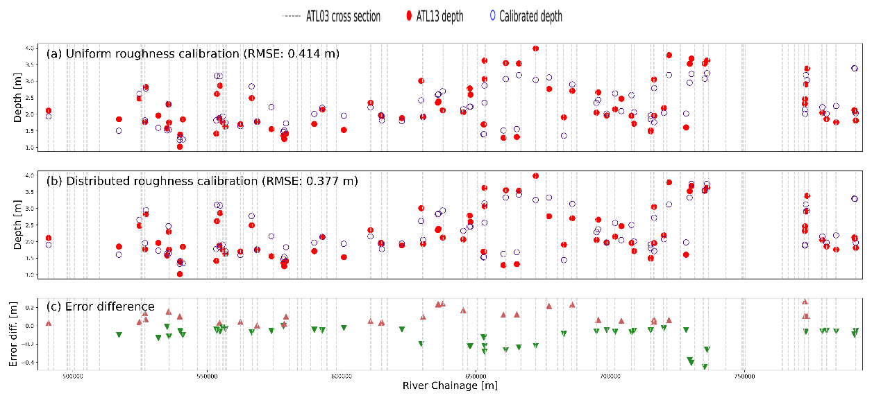
Figure A1 Uniform depth calibration (a) compared with the distributed roughness calibration for eight Manning's roughness values (b) and the error difference between the uniform calibration and the distributed calibration (c).

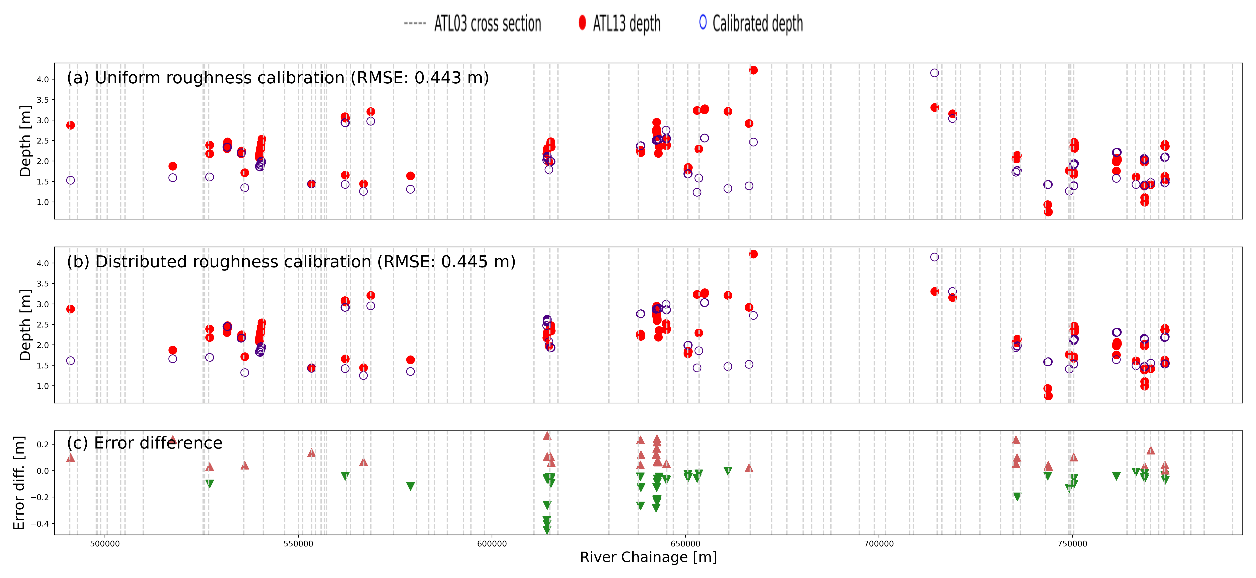
Figure A2 Validation data error for uniform depth calibration (a), distributed roughness calibration for eight Manning's roughness values (b), and the error difference between the uniform calibration and the distributed calibration (c).

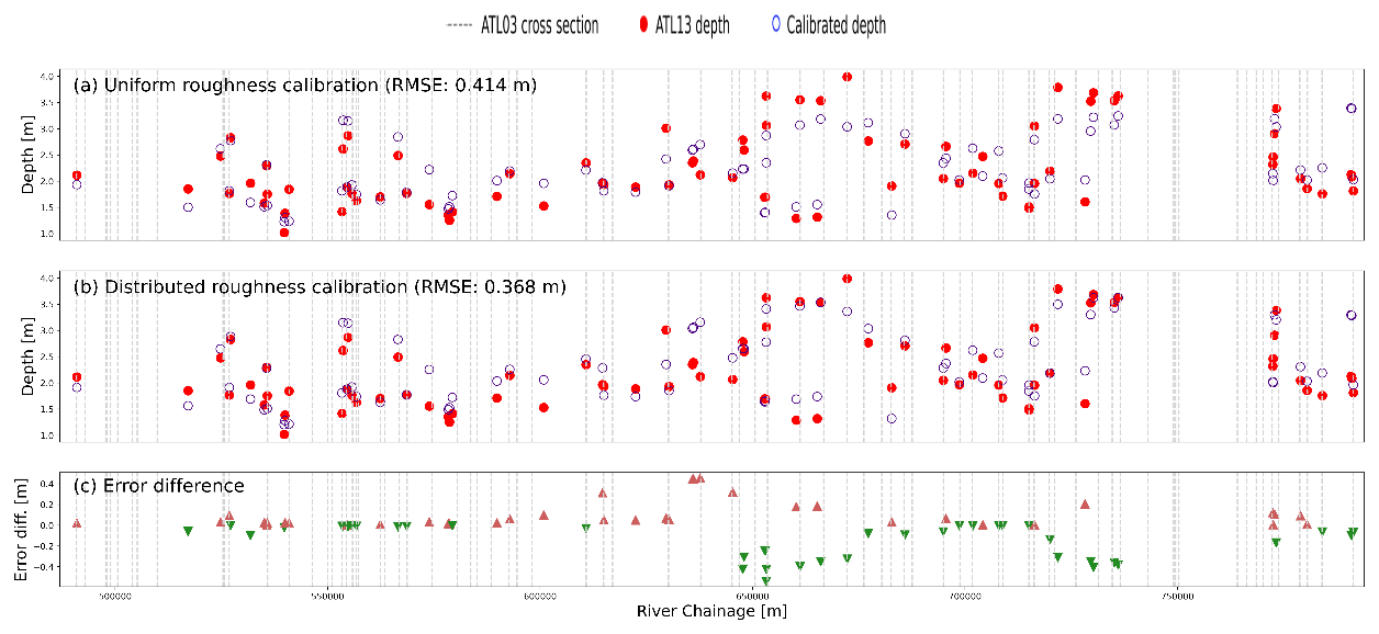
Figure A3 Uniform depth calibration (a) compared with distributed roughness calibration for 16 Manning's roughness values (b) and the error difference between the uniform calibration and the distributed calibration (c).

Figure A4 Validation data error for uniform depth calibration (a), distributed roughness calibration for 16 Manning's roughness (b), and error difference between the uniform calibration and the distributed calibration (c).