Reconstructing climate trends adds skills to seasonal reference crop evapotranspiration forecasting

Evapotranspiration plays an important role in the terrestrial water cycle. Reference crop evapotranspiration (ET_o) has been widely used to estimate water transfer from vegetation surface to the atmosphere. Seasonal ET_o forecasting provides valuable information for effective water resource management and planning. Climate forecasts from general circulation models (GCMs) have been increasingly used to produce seasonal ET_o forecasts. Statistical calibration plays a critical role in correcting bias and dispersion errors in GCM-based ET_o forecasts. However, time-dependent errors resulting from GCM misrepresentations of climate trends have not been explicitly corrected in ET_o forecast calibrations. We hypothesize that reconstructing climate trends through statistical calibration will add extra skills to seasonal ET_o forecasts. To test this hypothesis, we calibrate raw seasonal ET_o forecasts constructed with climate forecasts from the European Centre for Medium-Range Weather Forecasts (ECMWF) SEAS5 model across Australia, using the recently developed Bayesian joint probability trend-aware (BJP-ti) model. Raw ET_o forecasts demonstrate significant inconsistencies with observations in both magnitudes and spatial patterns of temporal trends, particularly at long lead times. The BJP-ti model effectively corrects misrepresented trends and reconstructs the observed trends in calibrated forecasts. Improving trends through statistical calibration increases the correlation coefficient between calibrated forecasts and observations (r) by up to 0.25 and improves the continuous ranked probability score (CRPS) skill score by up to 15 (%) in regions where climate trends are misrepresented by raw forecasts. Skillful ET_o forecasts produced in this study could be used for streamflow forecasting, modeling of soil moisture dynamics, and irrigation water management. This investigation confirms the necessity of reconstructing climate trends in GCM-based seasonal ET_o forecasting and provides an effective tool for addressing this need. We anticipate that future GCM-based seasonal ET_o forecasting will benefit from correcting time-dependent errors through trend reconstruction.

1 Introduction

As a critical process in the terrestrial water cycle, evapotranspiration transfers a large amount of water from the land surface to the atmosphere. Reference crop evapotranspiration (ET_o) measures the evaporative demand of the atmosphere for a hypothetical crop of a given height with defined surface resistance factor and albedo. It is generally computed using the Penman–Monteith equation, following Allen et al. (1998, see Sect. 2.1), which is known as FAO56. McMahon et al. (2013) provide additional information about the process. Forecasting of ET_o has been used to support water resource management (Anderson et al., 2015; Le Page et al., 2021) and improve soil moisture modeling (Yu et al., 2016). In addition, ET_o forecasting also helps constrain the significant uncertainties in streamflow forecasting (Greuell et al., 2019; Van Osnabrugge et al., 2019). Seasonal ET_o forecasts have been used to support water allocation among competing users (Chauhan and Shrivastava, 2009) and in planning farming activities (Zinyengere et al., 2011). In recent years, climate forecasts produced by general circulation models (GCMs) have been increasingly used for seasonal ET_o forecasting, since GCMs often produce forecasts of all climate variables needed to estimate future ET_o (Tian et al., 2014; Zhao et al., 2019a).

Raw ET_o forecasts constructed with GCM climate forecasts often inherit significant errors from the raw forecasts of climate variables, including temperature, solar radiation, wind speed, and vapor pressure. Due to deficiencies in the GCM representation of physical processes of the atmosphere (Woldemeskel et al., 2014), model parameterization (O'Gorman and Dwyer, 2018), and data assimilation (O'Kane et al., 2019), raw GCM forecasts often demonstrate systematic errors (Weisheimer and Palmer, 2014). For example, inconsistencies with observations have been reported for the raw forecasts of all variables needed to construct ET_o forecasts using the FAO56 method (Groisman et al., 2000; Slater et al., 2017). These inconsistencies often lead to significant bias and low skills in the resultant raw ET_o forecasts (Zhao et al., 2019b).

Failing to correctly simulate the temporal trends of the climate system could be partially responsible for the low skills of GCM-based raw ET_o forecasts. Time-dependent errors are introduced when GCMs lack skills in modeling climate trends driven by rising atmospheric greenhouse gas (GHG) concentrations (Sansom et al., 2016). There is mounting evidence that climate change has resulted in increasing trends in temperature (Smith et al., 2007) and vapor pressure (Byrne and Gorman, 2018) but led to decreasing trends in solar radiation (Liepert, 2002). However, GCMs configured for seasonal climate forecasts often misrepresent these observed trends. For example, an evaluation across nine climate regions in the U.S. showed that nine of 10 selected GCMs failed to reproduce the observed temporal trends in seasonal temperature forecasts (Das Bhowmik and Sankarasubramanian, 2020). In the Middle East, seasonal temperature forecasts by the Climate Forecast System Version 2 (CFSv2) model overestimated the warming trend in reference data by approximately 0.4^∘C per decade (Alizadeh-Choobari et al., 2019). In Australia, evaluations of the European Centre for Medium-Range Weather Forecasts (ECMWF) SEAS5 model identified significant discrepancies between observed and forecasted trends in temperature (Shao et al., 2020, 2021). Forecasts of the fire weather index (calculated with forecasts of precipitation, wind speed, temperature, and humidity), based on the ECMWF System 4 model, demonstrated significant inconsistencies with observations in temporal trends in Europe during 1981–2010 (Bedia et al., 2018). As a result, it is unlikely that raw ET_o forecasts constructed with raw forecasts of these climate variables would faithfully reproduce the observed climate trends. Failing to capture the observed trends inevitably introduces errors to GCM-based raw ET_o forecasts.

Raw ET_o forecasts constructed with climate forecasts need to be calibrated to correct biases and dispersion errors. Statistical calibration models initially developed for other variables, such as precipitation or temperature, have been adopted to calibrate raw ET_o forecasts (Medina and Tian, 2020; Zhao et al., 2019a). Using a quantile mapping method, Tian et al. (2014) improved seasonal ET_o forecasts based on CFSv2 outputs in Florida, USA. In the calibration of seasonal ET_o forecasts in Australia, Zhao et al. (2019b) used the Bayesian joint probability (BJP) model to post-process ET_o forecasts constructed with climate forecasts from the Australian Bureau of Meteorology's Australian Community Climate and Earth-System Simulator–Seasonal prediction system version 1 (ACCESS-S1) model across three weather stations. This investigation validated the BJP model's strengths in error correction and skill enhancement in ET_o forecasting. However, none of these calibrations have explicitly dealt with time-dependent errors caused by the misrepresentation of climate trends in GCM forecasts.

Statistical techniques have been developed to correct time-dependent errors in raw GCM forecasts. A commonly adopted method is to replace the linear trend in raw forecasts with the observed trend (Kharin et al., 2012). Using this method, Kharin et al. (2012) corrected trends in decadal temperature forecasts and successfully reduced the systematic residual drifts in raw forecasts. Meanwhile, improvements in trends effectively adjusted the long-term climate behavior in forecasts to match the observations (Kharin et al., 2012). To correct errors associated with the representation of temporal changes and variability, Pasternack et al. (2021) adopted a time-varying mean to characterize the climate trend in the calibration of decadal temperature forecasts. In addition to these decadal-scale calibrations, recent studies suggested that seasonal climate forecasting could also benefit from correcting time-dependent errors. For example, Shao et al. (2021) improved the BJP model by adding trend reconstruction algorithms to deal with time-dependent errors. The new algorithm allows for the reconstruction of observed trends in calibrated forecasts. With this new feature, the improved BJP model (hereafter referred to as BJP-ti) demonstrates the capability of adding extra skills to seasonal temperature forecasts through trend reconstruction.

We hypothesize that reconstructing trends in seasonal ET_o forecasts through statistical calibration will help correct time-dependent errors and, thereby, improve the forecast skills. To test this hypothesis, we adopt the BJP-ti model to calibrate seasonal ET_o forecasts constructed with climate forecasts from the ECMWF SEAS5 model across Australia. This investigation aims to (1) reconstruct climate trends in seasonal ET_o forecasts through statistical calibration and (2) investigate how trend reconstruction affects the skill of calibrated ET_o forecasts.

2 Method

2.1 Observations and forecasts

We develop monthly ET_o data (treated as observations for calibration) based on gridded monthly temperature, solar radiation, and vapor pressure data from the Australian Water Availability Project (AWAP; Jones et al., 2007, 2014). Since the AWAP does not provide wind speed data, we use a constant wind speed of 2 m s⁻¹ in deriving the ET_o observations (Allen et al., 1998). Based on these AWAP variables, we produce monthly ET_o observations during 1990–2019 for forecast calibration.

Seasonal climate forecasts from the latest version (SEAS5) of the ECMWF model are used to construct the raw ET_o forecasts. The re-forecast period of SEAS5 is 1981–2016, with an ensemble size of 25 members. Real-time forecasts started in 2017, with an ensemble size of 51 members (Stockdale et al., 2017). SEAS5 forecasts have a horizon of 7 months (months 0 to 6), with a spatial resolution of 0.4^∘. While SEAS5 produces climate forecasts across the globe, the calibration in this study is performed across Australia only.

To match ET_o observations, we combine the archived re-forecasts and operational forecasts to derive raw ET_o forecasts for the period of 1990–2019. ECMWF runs for re-forecasts and operational forecasts are configured in a similar way, except for differences in initialization (Johnson et al., 2019). Absolute errors in raw ET_o forecasts during the two periods are comparable (Fig. S1 in the Supplement). We choose the first 25 ensemble members of the real-time forecasts (2017–2019) to match the ensemble size of the re-forecasts (1990–2016). We calculate the ensemble mean of the 25 ensemble members of ECMWF forecasts of temperature, solar radiation, and vapor pressure for the calculation of raw ET_o forecasts. To be consistent with the ET_o observations, we use a constant wind speed of 2 m s⁻¹ in deriving raw ET_o forecasts. In addition, we aggregate the grid spacing of AWAP data from 0.05 to 0.4^∘ to match the ECMWF's spatial resolution.

2.2 Calculation of ET_o observations and forecasts

We construct monthly raw ET_o forecasts and ET_o observations using the monthly ECMWF climate forecasts and AWAP data based on the FAO56 ET_o method as follows (Allen, et al., 1998):

$$\begin{array}{}\text{(1)}& {\text{ET}}_{\mathrm{o}}={\displaystyle \frac{\mathrm{0.408}\mathrm{\Delta }\left(R_{\mathrm{n}}-G\right)+\mathit{\gamma }\frac{\mathrm{900}}{T+\mathrm{273}}{u}_{\mathrm{2}}\left(e_{\mathrm{s}}-e_{\mathrm{a}}\right)}{\mathrm{\Delta }+\mathit{\gamma }(\mathrm{1}+\mathrm{0.34}{u}_{\mathrm{2}})}},\end{array}$$

where ET_o is the monthly reference crop evapotranspiration (millimeters per month), Δ is the slope of the vapor pressure curve (kPa ^∘C⁻¹), R_n is net radiation at the crop surface (MJ m⁻² per month), G is the soil heat flux density (MJ m⁻² per month), which is calculated based on temperature, γ is the psychrometric constant (kPa ^∘C⁻¹), T is average air temperature (^∘C), u₂ is the wind speed at 2 m (m s⁻¹), and e_s and e_a are saturated and actual vapor pressure (kPa), respectively.

2.3 Forecast calibration with the BJP-ti model

In this study, ET_o forecast calibration is conducted separately across Australia for each grid cell, month, and lead time. We employ the BJP-ti model to calibrate the raw ET_o forecasts. This model was developed recently by extending the original BJP model's capability to deal with errors resulting from the misrepresentation of climate trends. In this study, the calibration model is configured by month k (k=1 to 12, corresponding to January to December) of the year.

Calibration with the BJP-ti model involves six steps, including (1) transformation of the data, (2) detrending of the data, (3) joint probability modeling of the transformed and detrended forecasts and observations, (4) generation of ensemble calibrated forecast members conditional on the raw forecast, (5) addition of the observed trend back to ensemble members, and (6) back-transformation of the data to obtain the final calibrated forecasts. We further introduce these steps in detail, in the following.

The first step is to transform raw forecasts and observations to approach the normal distribution. We adopt the Yeo–Johnson transformation method (Yeo and Johnson, 2000) to transform ET_o as follows:

$$\begin{array}{}\text{(2)}& x{}^{\prime }=\left\{\begin{array}{ll}{\left(\mathit{\lambda }x+\mathrm{1}\right)}^{\frac{\mathrm{1}}{\mathit{\lambda }}}-\mathrm{1},& \left(x\ge \mathrm{0},\mathit{\lambda }\ne \mathrm{0}\right)\\ \exp \left(x\right)-\mathrm{1},& \left(x\ge \mathrm{0},\mathit{\lambda }=\mathrm{0}\right)\end{array}\right.,\end{array}$$

where λ is a transformation parameter, x refers to raw ET_o forecasts or ET_o observations (millimeters per month), and x^′ is the transformed x (forecasts or observations) generated through the Yeo–Johnson transformation. The above transformation is separately performed by month for raw forecasts and observations. The transformation parameter (λ) is inferred using the Bayesian maximum a posteriori (MAP) method (Shao et al., 2020).

Step 2 is to generate detrended forecasts and observations in the transformed space. For each grid cell, we separately infer linear trends for transformed forecasts and observations. With the trend parameters (α_f and α_o), the trends in transformed forecasts and observations are removed to produce detrended data. Specifically, each transformed forecast and observation record is adjusted based on the middle year of the study period (1990–2019) and trend parameters, using the following equations:

$$\begin{array}{}\text{(3)}& {\displaystyle }{z}_{\mathrm{f}}\left(t\right)=y{{}^{\prime }}_{\mathrm{f}}\left(t\right)-{\mathit{\alpha }}_{\mathrm{f}}(t-t_{\mathrm{m}}),\text{(4)}& {\displaystyle }{z}_{\mathrm{o}}\left(t\right)=y{{}^{\prime }}_{\mathrm{o}}\left(t\right)-{\mathit{\alpha }}_{\mathrm{o}}(t-t_{\mathrm{m}}),\end{array}$$

where $y{{}^{\prime }}_{\mathrm{f}}\left(t\right)$ and $y{{}^{\prime }}_{\mathrm{o}}\left(t\right)$ refer to the transformed ET_o forecasts and observations for month k (k=1 to 12, corresponding to January to December) in year t during 1990–2019. α_f and α_o are inferred trend parameters for transformed forecasts and observations, respectively. t_m is approximately the middle year (e.g., 2004 in this study) during 1990–2019. The position of t_m is empirically selected, but it will not affect the calibration if we choose a different year, as t_m, and z_f(t) and z_o(t) are detrended ET_o forecasts and observations in the transformed space, respectively.

In step 3, we assume a bivariate joint distribution (z) between the predictor z_f (detrended transformed raw forecasts) and predictand z_o (detrended transformed observations) as follows:

$$\begin{array}{}\text{(5)}& z=\left[\begin{array}{c}{z}_{\mathrm{f}}\\ z_{\mathrm{o}}\end{array}\right]\sim N\left(\mathit{\mu },\mathrm{\Sigma }\right),\end{array}$$

where μ is the mean vector, and Σ is the covariance matrix. We denote the parameters from Eqs. (3)–(5) as a vector $\mathit{\theta }=\left\{\mathit{\mu },\mathrm{\Sigma },{\mathit{\alpha }}_{\mathrm{f}},{\mathit{\alpha }}_{\mathrm{o}}\right\}$.

For each month of the year, model parameters are inferred with training data pairs (predictor and predictand) during the study period (1990–2019). The a posteriori distribution of the model parameters is as follows:

$$\begin{array}{}\text{(6)}& p\left(\mathit{\theta }\mathrm{|}D\right)\propto p\left(\mathit{\theta }\right)p\left(D\mathrm{|}\mathit{\theta }\right)=p\left(\mathit{\theta }\right){\prod }_{t=\mathrm{1}}^{n}p\left(D\mathrm{|}\mathit{\theta }\right),\end{array}$$

where p(θ) is the prior distribution for model parameters, and p(D|θ) is the likelihood function. D refers to all data pairs (z_f(t) and z_o(t)) used for parameter inference. A Gibbs sampler is utilized to repeatedly sample the parameter sets θ from the conditional a posteriori distribution of the model parameters.

In the BJP-ti model, informative priors are applied to set boundaries for inferred trends to avoid over-fitting. The priors are separately estimated for each grid cell, month, and lead time. This informative prior distribution p(α_i) for trend parameters α_f and α_o is formulated as follows (Shao et al., 2021):

$$\begin{array}{}\text{(7)}& p\left({\mathit{\alpha }}_i\right)\propto N(\mathrm{0},m_i^{\mathrm{2}})\end{array}$$

$$\begin{array}{}\text{(8)}& \begin{array}{rl}\left[{\mathit{\alpha }}_i\mathrm{|}\cdot \right]=& N\left({\displaystyle \frac{m_i^{\mathrm{2}}{\sum }_{t=\mathrm{1}}^n\left(y{{}^{\prime }}_i\left(t\right)-{\mathit{\mu }}_i\right)(t-t_{\mathrm{m}})}{m_i^{\mathrm{2}}{\sum }_{t=\mathrm{1}}^n(t-t_{\mathrm{m}}{)}^{\mathrm{2}}+{\mathit{\sigma }}_i^{\mathrm{2}}}}\right.,\\ & \left.{\displaystyle \frac{m_i^{\mathrm{2}}{\mathit{\sigma }}_i^{\mathrm{2}}}{m_i^{\mathrm{2}}{\sum }_{t=\mathrm{1}}^n(t-t_{\mathrm{m}}{)}^{\mathrm{2}}+{\mathit{\sigma }}_i^{\mathrm{2}}}}\right),\end{array}\end{array}$$

where m_i is the standard deviation of the prior, which is set based on trends of transformed forecasts and observations, μ_i is the mean, and σ_i is the standard deviation for predictors or predictands extracted from the diagonal of covariance matrix Σ (see Eq. 5). Equation (8) shows the a posteriori distribution of the parameter α_i conditional on forecasts or observations. For trends that are insignificant (P>0.05), we set m_i to 0 to avoid over-fitting trends in calibrated forecasts. For significant trends, we set the m_i value based on trends in observations and raw forecasts during 1981–2019. Specifically, we pooled the significant trends of all grid cells, months, and lead times for transformed forecasts and found that 95 % of the absolute trends are smaller than 0.47. For transformed observations, 95 % of grid cells and months have absolute trends less than 0.52. As a result, we set m_i to 0.47 and 0.52 for forecasts and observations, respectively.

In step 4, once all the parameters are inferred, we draw 1000 members from a conditional distribution of the predictand, (z_o(t^∗)), for a given new forecast, (z_f(t^∗)). In step 5, we add the trend from Eq. (4) back to z_o(t^∗) to produce a calibrated ensemble forecast $\left(y{{}^{\prime }}_{\mathrm{o}}\right(t^{\ast }\left)\right)$. In step 6, we back-transform $y{{}^{\prime }}_{\mathrm{o}}\left(t^{-}\right)$ to the original space to produce the calibrated ensemble forecasts. Our analysis indicated that our trend reconstruction strategy (detrending and retrending in the transformed space and setting limits to inferred trends) would not introduce significant bias to the calibrated forecasts (Fig. S2).

2.4 Evaluation of forecast calibration

To evaluate the performance of the calibration, we adopt a leave-1-year-out cross-validation strategy for each grid cell and lead time. Specifically, for one of the 30 years during 1990–2019, we keep month k aside and then use month k from the remaining 29 years to infer the BJP-ti parameters. Once the parameters are inferred, we generate a calibrated forecast for month k in the year held aside. This process is repeated until calibrated forecasts are obtained for month k from each of the 30 years. Similar processes are conducted for other months and other lead times until we obtain calibrated forecasts for all months and the seven lead times for each grid cell across Australia.

To evaluate how the reconstruction of trends affects the quality of calibrated forecasts, we compare BJP-ti calibrated forecasts with those generated using the original BJP model, which does not reconstruct trends. The BJP model omits steps 2 (detrending) and 5 (retrending) in Sect. 2.3. We present the results of the comparison in the main text for months (August, September, and October) with large areas (Fig. S3) of statistically significant (at the 95 % confidence interval) temporal trends in observed ET_o; the results for the remaining 9 months are presented in the Supplement.

Evaluation metrics employed to examine the performance of calibrations include the correlation coefficient, skill score, bias, and reliability. The calculation of these metrics is further introduced as follows.

2.4.1 Correlation coefficient

We use the Pearson correlation coefficient (r) between raw/calibrated forecasts and observations to examine their consistency in temporal dynamics as follows:

$$\begin{array}{}\text{(9)}& r={\displaystyle \frac{\sum _{t=\mathrm{1}}^n\left(x\right(t)-\stackrel{\mathrm{‾}}{x})\left(y\right(t)-\stackrel{\mathrm{‾}}{y})}{\sqrt{\sum _{t=\mathrm{1}}^n\left(x\right(t)-\stackrel{\mathrm{‾}}{x}{)}^{\mathrm{2}}}\sqrt{\sum _{t=\mathrm{1}}^n\left(y\right(t)-\stackrel{\mathrm{‾}}{y}{)}^{\mathrm{2}}}}},\end{array}$$

where x(t) is the ensemble mean of raw/calibrated ET_o forecasts (millimeters per month), n is the total years during the study period, $\stackrel{\mathrm{‾}}{x}$ is the average of x(t) (millimeters per month), y(t) is the corresponding ET_o observations (millimeters per month), and $\stackrel{\mathrm{‾}}{y}$ is the average of y(t) (millimeters per month).

2.4.2 Forecast skills

We use the continuous ranked probability score (CRPS) to measure the skill of the raw and calibrated forecasts as follows (Grimit et al., 2006):

$$\begin{array}{}\text{(10)}& {\displaystyle }\text{CRPS}\left(t\right)=\int {\left\{F(t,x)-H(x-y(t\left)\right)\right\}}^{\mathrm{2}}\mathrm{d}x,\text{(11)}& {\displaystyle }\stackrel{\mathrm{‾}}{\text{CRPS}}={\displaystyle \frac{\mathrm{1}}{n}}\sum _{t=\mathrm{1}}^n\text{CRPS}\left(t\right),\end{array}$$

where F(t,x) is the cumulative density function of an ensemble forecast, and y(t) is the observation at time t. H is the Heaviside step function (H=1 if $x-y\left(t\right)\ge \mathrm{0}$, and H=0 otherwise), and the overline represents averaging across the n months during January 1990–December 2019. For deterministic raw forecasts, CRPS is reduced to absolute errors.

We further calculate the CRPS skill score (CRPS_SS) to measure the skill of raw and calibrated forecasts relative to climatology forecasts using the following equation:

$$\begin{array}{}\text{(12)}& {\text{CRPS}}_{\mathrm{SS}}={\displaystyle \frac{{\text{CRPS}}_{\mathrm{reference}}-{\text{CRPS}}_{\mathrm{forecasts}}}{{\text{CRPS}}_{\mathrm{reference}}}}\times \mathrm{100},\end{array}$$

where CRPS_reference is the CRPS value of climatology forecasts, and CRPS_forecasts refers to CRPS value of raw or calibrated forecasts. Positive CRPS_SS indicates better skill than the climatology forecasts and vice versa. To make the CRPS skill scores of calibrated forecasts generated by different models (BJP vs. BJP-ti) comparable, we use the climatology forecasts from the BJP model as the reference in the calculation of CRPS_SS.

2.4.3 Bias

We evaluate the accuracy of the raw and calibrated forecasts using the following equation:

$$\begin{array}{}\text{(13)}& \text{Bias}={\displaystyle \frac{\mathrm{1}}{n}}{\sum }_{t=\mathrm{1}}^n\left(x\right(t)-y(t\left)\right),\end{array}$$

where Bias refers to the bias in ET_o (millimeters per month), n is total months during the 30-year study period (January 1990–December 2019), x(t) is the raw or calibrated forecasts of ET_o (millimeters per month), and y(t) is the corresponding ET_o observations of the same month (millimeters per month). Raw forecasts are deterministic since they are calculated based on the ensemble mean of each input variable. For calibrated forecasts, we use the ensemble mean to calculate bias.

2.4.4 Reliability

To evaluate the reliability of calibrated ensemble forecasts, we calculate the probability integral transform (PIT) value using the following equation:

$$\begin{array}{}\text{(14)}& \mathit{\pi }\left(t\right)=F\left(t,x=y\left(t\right)\right),\end{array}$$

where F(t,x) is the cumulative density function of the ensemble forecast, and y(t) is the observation. For reliable forecasts, the collection of π(t) follows a standard uniform distribution. We use the alpha (α) index to summarize the reliability in each grid cell with the following equation to check the overall reliability across Australia (Renard et al., 2010):

$$\begin{array}{}\text{(15)}& \mathit{\alpha }=\mathrm{1}-{\displaystyle \frac{\mathrm{2}}{n}}{\sum }_{t=\mathrm{1}}^n\left|{\mathit{\pi }}^{\ast }\left(t\right)-{\displaystyle \frac{t}{n+\mathrm{1}}}\right|,\end{array}$$

where π^*(t) is the sorted π(t), $t=\mathrm{1},\mathrm{2},\mathrm{\dots }n$ in ascending order, and n is the total number of months. The α index measures the total deviation of calibrated forecasts from the corresponding uniform quantile. Perfectly reliable forecasts should have an α index of 1, and forecasts with no reliability would have an α index of 0.

3 Results

3.1 Trends in observations and raw/calibrated forecasts

We evaluate the capability of BJP-ti in reconstructing temporal trends for months with large areas of statistically significant trends in observed ET_o. Since the trend parameters are estimated by month, we first examine the trend in ET_o observations for each month k of the year for 1990–2019 (Fig. S3). August, September, and October show larger areas with statistically significant trends than other months. As a result, the evaluation of trends in raw/calibrated forecasts is mainly conducted for these 3 months.

Figure 1 Trends in raw forecasts, BJP calibrated forecasts, and BJP-ti calibrated forecasts at month 0 and observed ET_o in August, September, and October. Blue polygons show regions where observed trends are statistically significant. SD refers to the standard deviation.

Observed ET_o shows increasing trends in many parts of Australia in the 3 selected months (Fig. 1; fourth column). Compared with findings from previous investigations, observed trends identified in this study also demonstrate significant spatial variability and varying magnitudes in different months (Donohue et al., 2010; McVicar et al., 2012). We found more positive trends in our study period (1990-2019) than the period of 1981–2006 (Donohue et al., 2010). In August, areas with increasing trends larger than 6 mm per decade are mainly located in the western parts of Australia. In contrast, central and eastern Australia demonstrates much lower trends of less than 4 mm per decade. Observed trends are close to zero in Victoria and Tasmania and even become negative in parts of the Northern Territory. In September, areas with significant increasing trends larger than 6 mm per decade are located in many parts of Australia, with the exception of a narrow coastal fringe and areas around the Tropic of Capricorn. In this month, decreasing trends are observed in a small part of the eastern areas of Western Australia, where observations are relatively poor. In October, central-eastern Australia, including the inland regions of Victoria, New South Wales, South Australia, and southwestern Queensland, demonstrate increasing trends of up to 8 mm per decade. At the decadal scale, trends in ET_o are comparable with the standard deviation.

Raw ET_o forecasts also demonstrate trends, but they differ from those in observations in both spatial patterns and magnitudes (left column in Fig. 1). In August, raw forecasts show increasing trends (>6 mm per decade) in Western Australia which partially match those in observations. However, in the eastern parts of Australia, raw forecasts overpredict trends in observations. In September, raw forecasts demonstrate even larger overpredictions (>8 mm per decade) in trends than those in August, particularly in Western Australia and New South Wales. In October, raw forecasts are better aligned with observations in the increasing trends in southeastern Australia; however, they overpredict trends in Western Australia and underpredict trends in northern Australia.

Trends in raw forecasts become weaker at longer lead times (left columns in Figs. S4 and S5). For the lead time of month 3, trends in raw ET_o forecasts show similar spatial patterns to those of month 0 in August but mainly drop to less than 2 mm per decade. Similarly, the magnitudes of increasing trends in the other 2 months are also much lower at month 3 than those at month 0. At month 6, trends in raw forecasts of the 3 selected months are close to zero across Australia.

Calibrated ET_o forecasts produced with the original BJP model demonstrate trends similar to those of raw forecasts in spatial patterns but show smaller magnitudes (second column in Figs. 1, S4, and S5, respectively). Specifically, at month 0, the BJP calibrated forecasts preserve the spatial variability in trends in the raw forecasts and show higher trends in Western Australia, the central parts of Australia, and the southern regions of the country for August, September, and October, respectively, but the increasing trends are all less than 4 mm per decade, which are lower than those in raw forecasts (Fig. 1). Consistencies in the spatial patterns of trends are also found between BJP calibrated forecasts and raw forecasts at other lead times (Figs. S4 and S5). Similarly, trends are also lower in BJP calibrated forecasts than those of the corresponding raw forecasts at longer lead times.

Calibration with the BJP-ti model successfully reconstructs the observed trends in the calibrated forecasts (third column in Figs. 1, S4, and S5, respectively). Inconsistencies between raw forecasts and observations in the spatial patterns and magnitudes of trends are effectively corrected through the calibration, particularly for regions that demonstrate significant observed trends. In addition, the tendency that trends become weaker at longer lead times in the raw forecasts is also effectively corrected. In the BJP-ti calibrated forecasts (third column in Figs. 1, S4, and S5, respectively), all lead times show trends consistent with observations in both spatial patterns and magnitudes.

3.2 Correlation coefficients between forecasts and observations

We further examine whether reconstructing trends improves the representation of ET_o temporal dynamics by forecasts. Specifically, we compare the r between BJP-ti calibrated forecasts and ET_o observations with those between BJP calibrated forecasts and observations in August, September, and October (Fig. 2). Following the trend reconstruction, BJP-ti calibrated forecasts clearly present temporal patterns more consistent with observations than calibrated forecasts produced by the BJP model, particularly in regions where observations show significant trends (Fig. S3) and for forecasts at longer lead times. For the lead time of month 0, increases in r of over 0.1 are mainly located in the coastal regions of northern Australia and northern Queensland for all 3 selected months. More significant improvements in r are found at longer lead times (months 3 and 6), with larger areas showing increases in r (Fig. 2). At month 3, in addition to the coastal areas in northern Australia, the majority of Western Australia shows increases in r by more than 0.2 in August; in September, significant increases in r occur in both the far north and far south of mainland Australia, and in October, areas with higher r further expand in southern Australia and cover much larger areas than those at month 0. Areas showing higher r continue to expand at month 6. In August, increases in r of over 0.2 or even 0.25 are found in the western and central parts of north Australia; in September, regions with higher r cover large areas in coastal parts of northern Australia and coastal regions across Victoria and South Australia. In October, r increases cover large areas of southern and central regions of Australia. Similar improvements are also found in the remaining 9 months (Fig. S6).

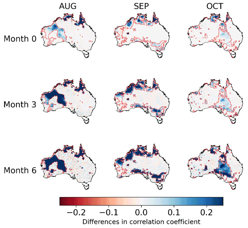
Figure 2 Differences in the correlation coefficient (r) between BJP-ti calibrated forecasts and observations with that between BJP calibrated forecasts and observations for 3 selected months (August, September, and October) and three lead times (months 0, 3, and 6). Red polygons show regions with significant observed trends.

3.3 Skills of raw and calibrated ET_o forecasts

Reconstruction of trends results in more skillful calibrated forecasts. We compare the CRPS skill scores of BJP-ti calibrated forecasts with those produced with the BJP model for the three selected months (Fig. 3). At month 0, the CRPS skill score of the calibrated forecasts is increased by 5 %–10 % in August, September, and October when trends are reconstructed. The distribution of areas with increased CRPS skill scores is generally consistent with that of the improved r (Fig. 2). Increases in the CRPS skill score are greater at longer lead times, in both magnitude and area, than those at short lead times. At month 3, areas with increased CRPS skill scores expand in Western Australia in August and in northern Western Australia in September. Month 6 demonstrates further improvements, with larger areas showing increases in the CRPS skill score of over 15 % in the coastal areas of northern Australia in August and September and central Australia in October. The other 9 months also demonstrate similar improvements in the CRPS skill score in regions with significant trends (Fig. S7). In addition, a comparison for all months together also demonstrates the improved skill score following the trend reconstruction (Fig. 4).

Figure 3 Differences in CRPS skill scores between BJP-ti calibrated forecasts and the BJP calibrated forecasts for 3 selected months (August, September, October) and three lead times (months 0, 3, and 6). Red polygons show regions with significant observed trends.

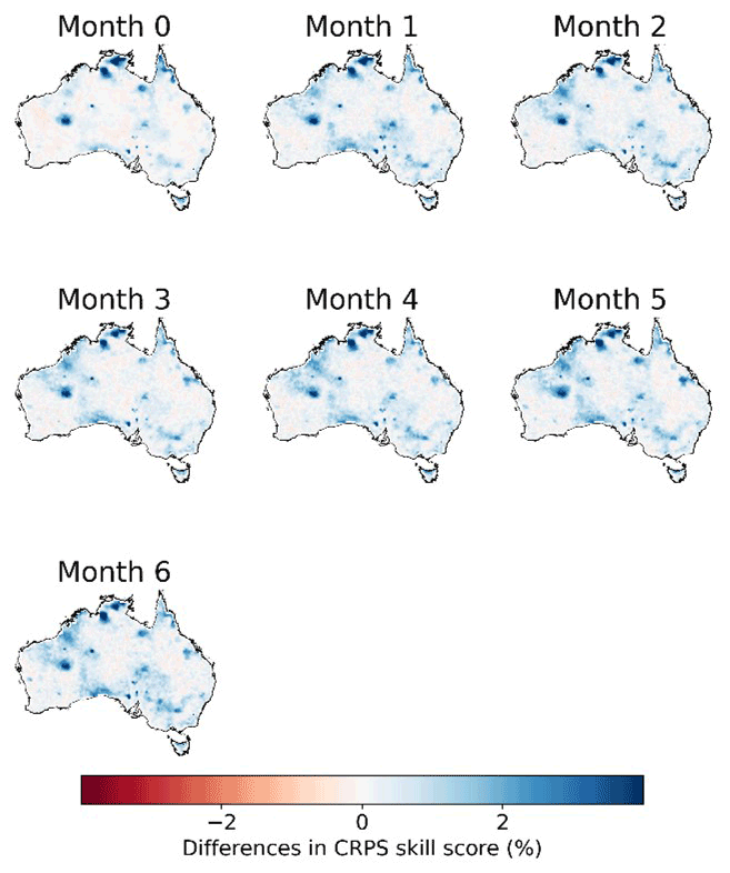
Figure 4 Differences in CRPS skill scores between BJP-ti calibrated forecasts and the BJP calibrated forecasts over 1990–2019.

We further evaluate the overall performance of the calibration over the whole study period by comparing the CRPS skill scores of the raw and BJP-ti calibrated forecasts (Fig. 5). Calibration with the BJP-ti model substantially improves the skills of the raw ET_o forecasts. Compared with the climatology forecasts, raw ET_o forecasts demonstrate much lower skills, with CRPS skill scores lower than −25 % in all grid cells, even for those at short lead times.

Figure 5 CRPS skill scores in (a) raw and (b) calibrated forecasts at seven lead times during 1990–2019.

We need to point out that simple bias correction is often applied to raw ECMWF forecasts before they are used. We applied quantile mapping to the raw ET_o forecasts and were able to improve forecast skills (Fig. S8). However, the bias-corrected forecasts still demonstrate skills much worse than climatology forecasts, particularly at long lead times.

With the correction of errors, including the time-dependent errors, the BJP-ti calibrated forecasts demonstrate CRPS skill scores larger than 20 (%) at month 0 in most grid cells (Fig. 5). The eastern parts of Australia, such as New South Wales and Victoria, show CRPS skill scores of up to 30 (%). Beyond month 0, the skill score decreases significantly in calibrated forecasts. Most areas of Australia show CRPS skill scores lower than 10 (%) at month 1. The skill score further decreases at longer lead times but remains above zero in many parts of Australia, even at month 6, suggesting better performances than the climatology forecasts.

We also summarize the CRPS skill score of calibrated forecasts by target month at the seven lead times across Australia (Fig. 6). Individual boxes indicate the variability among all the grid cells across Australia for that month and lead time. At the first lead time (month 0), all months show a CRPS skill score that is markedly better than the climatology forecasts across most grid cells, with the median CRPS skill score being above 20 (%) for 7 months. However, the skill score decreases quickly with lead time. At lead time 1, the CRPS skill score is mainly lower than 10 (%) for all target months. The skills of calibrated forecasts vary among the months. For October, November, and December, the CRPS skill score is above 0 for more than 50 % of grid cells, even at lead time 6, indicating better performance than the climatology forecasts. For other months, such as January, April, May, and June, the median CRPS skill score decreases to values slightly below 0 beyond the first lead time (month 0).

Figure 6 Box plot of CRPS skill score by target month in BJP-ti calibrated forecasts.

3.4 Bias in raw and BJP-ti calibrated ET_o forecasts

Raw monthly ET_o forecasts constructed with the raw climate forecasts of the ECMWF SEAS5 model demonstrate significant overpredictions (Fig. 7). Positive biases of over 15 mm per month occur in most parts of Australia, away from the coastal fringe, and Tasmania. Small areas with negative biases are found in the coastal margins of Queensland and Tasmania. The spatial patterns of bias in the raw ET_o forecasts are consistent across all seven lead times, demonstrating systemic errors in raw ET_o forecasts. The BJP-ti calibration substantially corrects the systematic errors in the raw forecasts, resulting in biases close to 0 in calibrated forecasts for all lead times (Figs. 7 and S9).

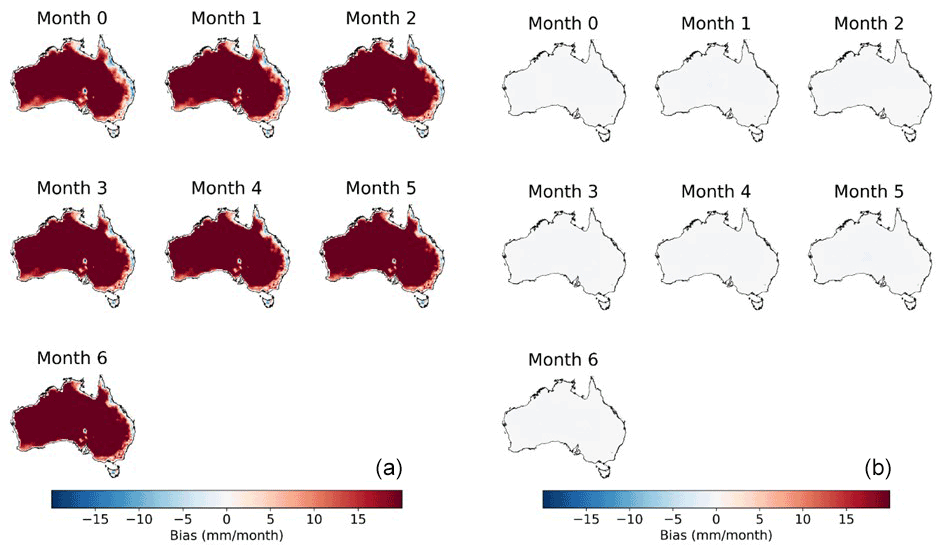
Figure 7 Bias in (a) raw and (b) BJP-ti calibrated ET_o forecasts.

3.5 Correlation between raw/calibrated forecasts and observations

The calibration based on the BJP-ti model also improves the correlation coefficients between forecasts and observations. Raw forecasts are able to capture the high seasonality in ET_o and, thus, demonstrate high correlation coefficients with observations (Fig. S10). The r values are generally over 0.9 across most parts of central and southern Australia. Lower r values are mainly distributed in coastal regions of northern Australia. Calibration with the BJP-ti model further improved the representation of the ET_o temporal dynamics (Fig. 8). The r values for the calibrated forecasts are over 0.9 in most parts of Australia. Improvements in r are more pronounced in northern Australia, where raw forecasts show lower correlations with observations.

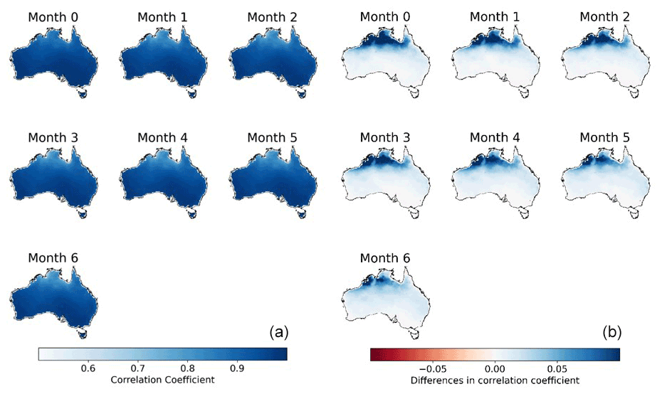
Figure 8 (a) Correlation coefficients between BJP-ti calibrated forecasts and observations and (b) improvements in correlation coefficients through the calibration with the BJP-ti model relative to those between raw forecasts and observations.

3.6 Reliability of calibrated ET_o forecasts

In this study, we generate 1000 ensemble members for each raw forecast to quantify the uncertainties of the calibrated forecasts. As indicated by the α index, calibrated ET_o forecasts are highly reliable. The α index of calibrated ensemble ET_o forecasts is above 0.96 in most parts of Australia for all the seven lead times (Figs. 9 and S11). The high reliability of the calibrated forecasts suggests reasonable representations of uncertainties in calibrated ET_o forecasts, and the distributions of calibrated ensemble forecasts are neither too narrow nor too wide (Fig. 9).

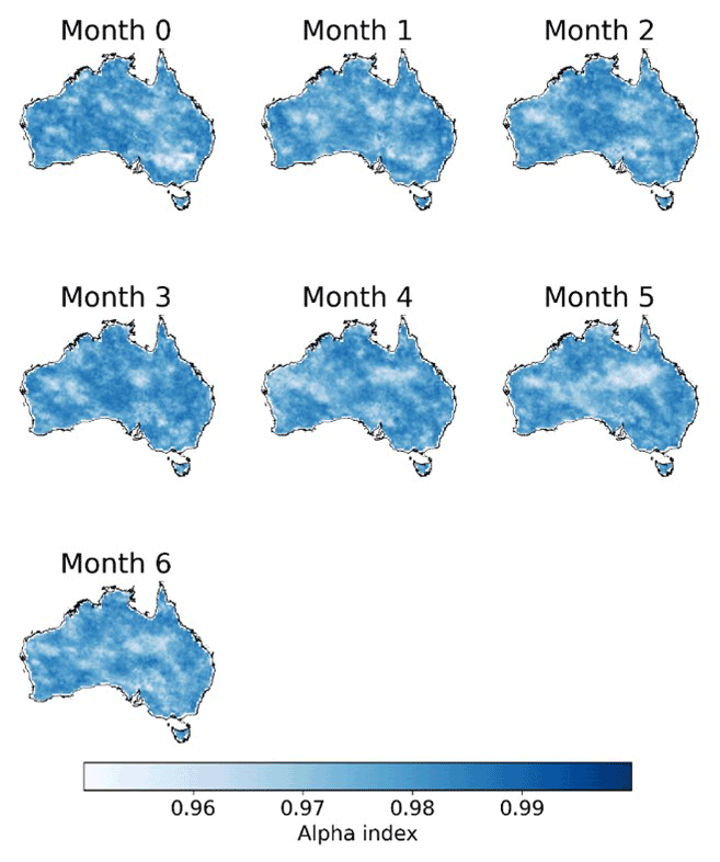
Figure 9 Alpha index of BJP-ti calibrated ensemble ET_o forecasts.

4 Discussion

4.1 The necessity of reconstructing climate trends in seasonal ET_o forecasting

This investigation confirms that the misrepresentation of climate trends is an important error source in GCM-based ET_o forecasting. Most previous investigations on climate trends in seasonal forecasts were primarily focused on temperature (Krakauer, 2019) and precipitation (Alizadeh-Choobari et al., 2019), and existing ET_o forecasting studies have not investigated trends in ET_o forecasts, despite temporal trends in ET_o being observed at weather stations across the globe (Djaman et al., 2018; Kousari and Ahani, 2012). Although the ECMWF model runs have been forced with the observed greenhouse gas concentrations for our study period (Johnson et al., 2019), and have actually produced temporal trends in raw ET_o forecasts (Fig. 1), the trends show significant inconsistencies with observations. In addition, raw ET_o forecasts at long lead times demonstrate much weaker trends than those at short lead times. Since misrepresentations of climate trends have been reported for many GCMs (Dunn et al., 2017), GCM-based seasonal ET_o forecasting may generally suffer from time-dependent errors.

This investigation also verifies our hypothesis that correcting time-dependent errors through trend reconstruction can add extra skills to calibrated ET_o forecasts. Reconstruction of climate trends using the BJP-ti model effectively improves the consistency between forecasts and observations in temporal patterns and leads to more skillful calibrated forecasts when compared with the calibration that does not reconstruct trends in ET_o forecasts. These improvements are particularly significant in regions showing statistically significant observed trends and at long lead times when trends are misrepresented most. Consequently, this investigation clearly indicates the necessity of correcting time-dependent errors in GCM-based seasonal ET_o forecasting. Although it may take decades for climate change to substantially alter the magnitude of ET_o (Figs. S11 and 12), we recommend that future GCM-based ET_o forecasting should still correct time-dependent errors. More frequent extreme weather events in recent years support model projections that climate change will intensify in the future (Kharin et al., 2013) and may induce more significant temporal trends in ET_o.

4.2 Implications for improving statistical calibration models

Climate change has posed challenges to the statistical calibration of seasonal climate forecasts. Many post-processing models, such as those based on the probabilistic theory (Tian et al., 2014; Wang et al., 2009), often rely on the climatology of observations to construct the probability distribution function for calibration (Wilks, 2018). However, the non-stationary behavior of the climate system induced by elevated greenhouse gas emissions has been increasingly reported (Haustein et al., 2016; Lima et al., 2015). Many calibration models developed for seasonal forecasts have not considered the climate change impacts on the observed climatology. Although these models are proven to be effective in correcting biases in raw forecasts, assuming a static climatology may have hindered the utilization of predictable information in the raw forecasts. This investigation and our previous calibration of seasonal temperature forecasts (Shao et al., 2020, 2021) suggest that reconstructing trends in calibrated forecasts is an effective solution for capturing the non-stationary behavior of the climate system for more robust statistical calibrations of seasonal climate forecasts.

This current investigation has further validated the strength of the trend reconstruction algorithms in BJP-ti. Previously, we applied this model to correct seasonal temperature forecasts and achieved significant improvements in forecast skills relative to the original BJP model (Shao et al., 2020, 2021). This study further demonstrates the feasibility of the general application of BJP-ti to different hydroclimate variables showing temporal trends (Shao et al., 2022a, b). The successful application to ET_o forecasts confirms the robustness of trend reconstruction algorithms based on the data transformation, Bayesian inference, and using the statistical significance of observed trends to deal with the over-fitting of trend parameters in the BJP-ti model. We also anticipate that the BJP-ti algorithms for trend reconstruction could be adopted by other calibration models to enhance seasonal forecast calibration.

4.3 Future work

In this investigation, we successfully improve ET_o forecast calibration by reconstructing climate trends. We also identify a few challenges that should be addressed in the future to further enhance GCM-based seasonal ET_o forecasting.

First of all, more sophisticated cross-validation methods should be developed for the inference of trend parameters. The current leave-one-out method has been proven to be effective in the inference of the mean vector and covariance matrix (Shao et al., 2020). However, this strategy may not guarantee the independence between the left-out data and the data used for the inference of trend parameters. We decided not to implement the data-splitting method for cross-validation because of the risk of introducing sampling errors. Future investigations should take this challenge into consideration and develop more robust cross-validation methods for the inference of trend parameters.

In this study, we directly use the raw forecasts of individual input variables (e.g., temperature, solar radiation, and vapor pressure) to construct the raw ET_o forecasts. However, trends in these variables have been reported in previous investigations. Whether correcting errors, including time-dependent errors in the raw forecasts of each input variable, will lead to more skillful calibrated ET_o forecasts, warrants further investigation.

Correction of lead-time-dependent errors should be further investigated in future GCM-based ET_o forecasting. We found sharp declines in the skill of calibrated ET_o forecasts from lead time month 0 to month 1. Model initialization with field observations plays a critical role in seasonal climate forecasting based on GCMs (Doblas-Reyes et al., 2013; Hazeleger et al., 2013). Short lead time forecasts are more skillful since they are closer to the observed state of the climate system than those at long lead times. At long lead times, the predictable signal is often much smaller than the intrinsic uncertainty of GCMs. As a result, the skills of raw forecasts often decrease quickly in the first month (Swapna et al., 2015), posing a challenge to statistical calibration, even for those using sophisticated calibration models (Hawthorne et al., 2013). Currently, we calibrate raw ET_o forecasts of each lead time independently. Whether correcting the lead-time-dependent biases will add extra skills to calibrated forecasts, particularly to those at long lead times, warrants further investigation (Van Schaeybroeck and Vannitsem, 2018).

Future forecast calibration should also investigate the impacts of climate change on the temporal variations in ET_o. In addition to the increasing or decreasing trends, warming climate also induced more significant temporal variations in ET_o, following increasing climate extremes (Wen et al., 2012). The increasing variations could pose another challenge to statistical calibration models, assuming an unchanged variance of the observations. This current investigation provides a remedy for dealing with the varying mean of ET_o in statistical calibration. Future investigations should evaluate whether allowing the variance to vary with time in calibration models would further improve the skills of seasonal ET_o forecasts.

5 Conclusions

ET_o forecasting provides useful information for hydrological investigations and has been increasingly used to support water resource forecasting and management. Anthropogenic disturbances have induced changes in the climate system and resulted in trends in many climate variables. GCMs often misrepresent these climate trends and, thus, lead to time-dependent errors in seasonal climate forecasts. We have recently improved the BJP model to deal with this error source through the reconstruction of observed climate trends in calibrated forecasts. In this study, we apply the BJP-ti model to calibrate raw seasonal ET_o forecasts constructed with climate forecasts from the ECMWF SEAS5 model. The BJP-ti model effectively corrects misrepresented climate trends and reconstructs observed trends in calibrated ET_o forecasts. More importantly, forecast skills in areas showing statistically significant observed trends in observations are improved following trend reconstruction. This investigation highlights the necessity of correcting time-dependent errors for enhancing GCM-based seasonal ET_o forecasting. We conclude that future ET_o forecasting based on GCM climate forecasts could improve forecast skills through reconstructing climate trends in forecasts.

This investigation also provides valuable insights for improving statistical calibrations of seasonal climate forecasts in the future. In recent decades, climate trends have been increasingly observed. However, many calibration models for seasonal forecasts have not taken the non-stationary behavior of the climate system into consideration. Improved forecast skills in seasonal ET_o forecasts through the reconstruction of temporal trends, together with our previous calibration of seasonal temperature forecasts, validate the robustness and effectiveness of trend reconstruction algorithms in the BJP-ti model. We anticipate that these algorithms would be applicable to enhance other calibration models.