Monitoring surface water dynamics in the Prairie Pothole Region of North Dakota using dual-polarised Sentinel-1 synthetic aperture radar (SAR) time series

The North American Prairie Pothole Region (PPR) represents a large system of wetlands with great importance for biodiversity, water storage and flood management. Knowledge of seasonal and inter-annual surface water dynamics in the PPR is important for understanding the functionality of these wetland ecosystems and the changing degree of hydrologic connectivity between them. Optical sensors that are widely used for retrieving such information are often limited by their temporal resolution and cloud cover, especially in the case of flood events. Synthetic aperture radar (SAR) sensors can potentially overcome such limitations. However, water extent retrieval from SAR data is often impacted by environmental factors, such as wind on water surfaces. Hence, robust retrieval methods are required to reliably monitor water extent over longer time periods .

The aim of this study was to develop a robust approach for classifying open water extent in the PPR and to analyse the obtained time series covering the entire available Sentinel-1 observation period from 2015 to 2020 in the hydrometeorological context. Open water in prairie potholes was classified by fusing dual-polarised Sentinel-1 data and high-resolution topographical information using a Bayesian framework. The approach was tested for a study area in North Dakota. The resulting surface water maps were validated using high-resolution airborne optical imagery. For the observation period, the total water area, the number of waterbodies and the median area per waterbody were computed. The validation of the retrieved water maps yielded producer’s accuracies between 84 % and 95 % for calm days and between 74 % and 88 % for windy days. User’s accuracies were above 98 % in all cases, indicating a very low occurrence of false positives due to the constraints introduced by topographical information.

The observed dynamics of total water area displayed both intra-annual and inter-annual patterns. In addition to differences in seasonality between small (<1 ha) and large (>1 ha) waterbodies due to the effect of evaporation during summer, these size classes also responded differently to an extremely wet period from 2019 to 2020 in terms of the increase in the number of waterbodies and the total area covered. The results demonstrate the potential of Sentinel-1 data for high-resolution monitoring of prairie wetlands. Limitations of this method are related to wind inhibiting the correct water extent retrieval and to the rather long acquisition interval of 12 d over the PPR, which is a result of the observation strategy of Sentinel-1.

1 Introduction

Surface water dynamics in wetland ecosystems play an important role in water storage variability of a region (Acreman, 2012) and are of great importance for flood management (Huang et al., 2011b), biodiversity (Cohen et al., 2016), groundwater recharge (Mitsch and Gosselink, 2000) and biogeochemical cycles (Cheng and Basu, 2017). The distribution of wetlands of different sizes in time and space is a key factor determining their function in a landscape. While large wetlands store considerable water volumes (Liu and Schwartz, 2011), small wetlands fulfil important roles for biodiversity by acting as habitats (Krapu et al., 2018). The ecological functioning of wetlands depends greatly on the abundance of wetlands of different sizes in the landscape, which is subject to land-use changes and climate variability (McKenna et al., 2019).

The Prairie Pothole Region (PPR) of North America covers an area of over 780 000 km² in the Great Plains of the northern USA and southern Canada. The region is characterised by millions of shallow depressions formed during glacier retreat at the end of the last glacial period when glacial till was unevenly deposited in ground moraines. These depressions contain wetlands whose areas vary between 1 m² and several square kilometres. They can store considerable amounts of water during rainfall events, which contributes to flood mitigation in downstream populated areas (Huang et al., 2011b). The wetlands of the region are of great importance for the waterfowl population of North America (Mitsch and Gosselink, 2000). Many of the smaller wetlands fall dry during the summer months, especially in drier years, and refill during spring snowmelt or intense rainfall events (Huang et al., 2011a; Montgomery et al., 2018). Thus, the waterbody size distribution of the PPR and its variability have attracted considerable interest in the hydrologic community (Bertassello et al., 2019; Liu and Schwartz, 2011; Proulx et al., 2013). Van Meter and Basu (2015) revealed a preferential loss of smaller wetlands when comparing current maps to historic data, which they attributed to the artificial draining of small, upland wetlands and to the preferential restoration of large, lowland wetlands. Furthermore, distances between individual wetlands as well as between wetlands and the river network have increased, with important implications for their connectivity, for example, in terms of habitat function. In another study, distributions of pothole sizes from a hydrological model run over the 20th century (Liu and Schwartz, 2011) were analysed with respect to their inter-annual and seasonal changes. The abundance of larger potholes (>1 ha) was found to be relatively unaffected by short-term climatic variations, whereas the size distribution of smaller wetlands changed due to the typical seasonal cycle of snowmelt in spring and gradual drying out due to high evaporation rates in summer.

Direct evidence to support such conceptual models of water surface dynamics in the PPR is mainly based on Earth observation (Rover and Mushet, 2015). Remote-sensing-based approaches can be used to derive wetland extent over large areas at a comparatively low cost (Ozesmi and Bauer, 2002). The resulting wetland extent maps have been used to calibrate and validate hydrological models simulating wetlands behaviour (McIntyre et al., 2014). Both optical and synthetic aperture radar (SAR) data have been used for mapping surface water extent in the PPR (Proulx et al., 2013; Vanderhoof et al., 2016; Brooks et al., 2018; Bolanos et al., 2016). In addition to satellite data, very high resolution (HR) airborne optical data and lidar data have been used both for estimating surface water extent and routing of water flow between potholes (Wu and Lane, 2017; Wu et al., 2019; Vanderhoof and Lane, 2019). However, satellite-based imagery has received the bulk of attention to date, likely due to its lower cost. Landsat imagery in particular has received much consideration due to its long time period covered (i.e. from 1972 to present). Vanderhoof et al. (2016) mapped inter-annual changes in wetland extent using time series of cloud-free Landsat scenes at an approximately annual interval over a 21-year period. Wetland extent and connectivity were found to correlate with each other as well as with climatological indices and runoff. The authors noted that their study was limited by the spatial resolution of the Landsat data and by the fact that sub-annual dynamics in small wetlands (e.g. in response to rainfall events) could not be assessed. In a study using eight Landsat scenes acquired over the course of 2 years, Brooks et al. (2018) found variations in total water surface area of ca. 50 % within a catchment. Although they analysed only a relatively small number of images, their results highlight the dynamic nature of surface water extent in the PPR. The use of Landsat imagery for monitoring surface water extent in the PPR is limited by its temporal resolution, which is additionally degraded by cloud cover, and its relatively coarse spatial resolution of 30 m (Rover and Mushet, 2015). In this context, Vanderhoof and Lane (2019) assessed the Landsat-based Global Surface Water (GSW) dataset (Pekel et al., 2016) for mapping the distribution of wetland sizes in the PPR and characterising their interactions. The authors concluded that analysis of the Landsat-based product alone would suggest that the landscape in the PPR is dominated by wetlands of sizes 0.2 to 8.0 ha. Using a dataset based on HR imagery that was pan-sharpened to a 0.5 m spatial resolution, however, resulted in smaller wetlands dominating the distribution of wetland sizes. Based on this product, they also detected narrow interactions between wetlands in the form of channels and locations where adjacent wetlands merged during wet periods (Vanderhoof and Lane, 2019).

However, HR satellite or airborne imagery is typically not available at the very short time intervals necessary to resolve intra-annual variations in waterbody sizes. Moreover, the flood mitigation potential of the wetlands in the PPR is a function of the water volume existing at the beginning of a flood event (Huang et al., 2011b). While cloud cover additionally limits the temporal resolution of optical data, SAR sensors have the potential to provide more continuous monitoring of the surface water extent. SAR data have been successfully used for wetlands mapping (e.g. Brisco, 2015; Reschke et al., 2012; Schlaffer et al., 2016; White et al., 2015). In addition to the ability of microwave radiation to penetrate clouds, SAR sensors are not only highly sensitive to the occurrence of open water surfaces (Richards, 2009) but also to flooding beneath vegetation (Tsyganskaya et al., 2018). Recent missions, such as Sentinel-1, also offer data at spatial resolutions comparable to or higher than Landsat and temporal sampling intervals in the order of several days. Open water surfaces act as specular reflectors and, as a result, appear dark in the resulting imagery (Giustarini et al., 2016). However, factors such as wind (Bartsch et al., 2012) or vegetation protruding through the water surface lead to an increase in the amount of energy scattered back to the sensor and, hence, increase false negative rates in the classification. Dry, sandy areas (Martinis et al., 2018), wet snow (Bartsch et al., 2012) or tarmac can be confused with open water during SAR image classification. In recent years, several studies have aimed at mapping and monitoring surface water dynamics in the PPR from SAR data (Bolanos et al., 2016; Huang et al., 2018; Montgomery et al., 2018). In particular, the analysis of polarimetric SAR data has received attention, as data acquired using different polarisations for sending and receiving (cross-polarised data) respond differently to scattering mechanisms, such as surface and volume scattering, than co-polarised data (same polarisation used for sending and receiving). Bolanos et al. (2016) used dual-polarised Radarsat-2 time series to map open water dynamics in the Canadian PPR and applied different thresholds to backscatter and image texture. Montgomery et al. (2018) analysed time series acquired by Radarsat-2 for classifying prairie wetlands according to their hydroperiod (i.e. the number of days per year that a wetland is covered by water). Strong fluctuations in water extent in accordance with precipitation inputs were reported, especially for the more hydrologically disconnected study sites. The rather long revisit cycle of Radarsat-2 of 24 d was mentioned as a major limiting factor for characterising surface water dynamics. In a study by Huang et al. (2018), data acquired by Sentinel-1, which has a temporal resolution of 12 d over most of the PPR, have been used to classify open water in the PPR of North Dakota. A set of polarised indices was created from the dual-polarised imagery and used together with backscatter coefficients as features in a random forest classifier trained on reference surface water products, such as the aforementioned GSW dataset. The authors noted that limitations of their approach relate to the omission of water-covered areas due to inundated vegetation and the spatial resolution of the sensor as well as commission errors due to smooth surfaces resembling open water in SAR imagery (Huang et al., 2018).

Such limitations, along with the short observation periods currently available for most SAR missions (in comparison to e.g. Landsat), pose the greatest hindrances for a wider uptake of SAR data for a long-term monitoring of wetland dynamics. In contrast to most SAR missions to date, the two-satellite Sentinel-1 constellation focuses on providing consistent data over longer time periods (Torres et al., 2012), which is ensured by the launch of Sentinel-1C/D planned from 2022 onwards (ESA CEOS EO Handbook, 2021). Therefore, there is a need for novel algorithms making use of the capabilities of Sentinel-1, such as dual polarisations and its high spatial temporal resolution, while addressing the above-mentioned limitations, such as misclassification due to water surfaces roughened by wind or land surfaces resembling open water. In the field of flood mapping, the inclusion of ancillary topographic information has been used to minimise the influence of these factors. Such ancillary information can be integrated into the classification workflow either by masking during post-processing (e.g. Westerhoff et al., 2013; Schlaffer et al., 2015) or by probabilistic data fusion of SAR and topographic data (e.g. D'Addabbo et al., 2016).

Here, a retrieval algorithm for open waterbodies in the PPR based on dual-polarisation Sentinel-1 data is proposed. We use a probabilistic approach based on Bayes' theorem combining SAR backscatter and information derived from a lidar-based digital elevation model in order to minimise the occurrence of false positives, caused by bare areas, tarmac or wet snow, which has been identified as a limiting factor in the aforementioned study (Huang et al., 2018). The method is applied to the full time series of Sentinel-1 imagery available for the snow-free months between 2015 and 2020. We hypothesise that a time series of water extent maps at sub-monthly intervals will facilitate the analysis of both intra-annual and inter-annual variations in the distribution of waterbody sizes. As mentioned earlier, modelling studies, such as Liu and Schwartz (2011), have demonstrated the sensitivity of small waterbodies to intra-annual variations, whereas larger waterbodies were only affected by deluge or drought periods at larger timescales. Our focus is on both the inter-annual surface water dynamics and the impacts of short, intense rainfall or snowmelt events on the number of waterbodies and the area covered by them. To our knowledge, this is the first time that inter-annual wetland dynamics in the PPR have been studied using the entire length of the Sentinel-1 time series. Furthermore, this study represents the first analysis of wetland dynamics during the flood events of 2019, which caused large areas in the Midwest to be inundated (Yin et al., 2020).

Figure 1 Digital elevation model of the Pipestem Creek catchment. The inset shows the location of the study area within the PPR. Dashed lines show the footprints of the aerial imagery used for validation. OpenStreetMap is used as the background. The elevation data are provided by the North Dakota State Water Commission (2018) under the Creative Commons license.

2 Material and methods

2.1 Study area

The study area comprises the Pipestem Creek catchment in North Dakota (ND), USA (Fig. 1). The catchment has an area of ca. 2770 km² and forms part of the PPR. The climate is continental with cold, dry winters (Wu and Lane, 2017) and a long-term average annual precipitation of approximately 440 mm (Huang et al., 2011a), most of which occurs during the summer months (Fig. 2a). Inter-annual precipitation variability is high: during the study period from 2015 to 2020, annual precipitation measured at Jamestown Regional Airport varied between 341 mm (in 2017) and 661 mm (in 2016). The study area is predominantly under agricultural use, and natural vegetation in the region mainly consists of grassland. According to the National Agricultural Statistical Service (NASS) Cropland Data Layer (CDL) for 2015 (USDA National Agricultural Statistics Service Cropland Data Layer, 2015), dominant crop types in the area are corn, soybean, wheat and sunflowers.

Discharge in the Pipestem Creek shows large variability (Fig. 2b). Runoff peaks typically occur in spring as a result of snowmelt; however, their magnitude varies considerably (e.g. between the spring seasons of 2016 and 2017). In 2019, runoff peaks occurred in both spring and autumn. In that year, ND and several other Midwestern states documented their wettest year on record. The high runoff led to widespread flooding in the Missouri, Arkansas and Mississippi river basins. In addition, blizzards in mid-October led to the declaration of a state-wide flood emergency (Umphlett, 2019). Between 2015 and 2018, the Palmer drought severity index (PDSI), which was derived from the Gridded Surface Meteorological Dataset (GRIDMET) (Abatzoglou, 2013) and averaged over the study area, oscillated between −2 and +2, indicating normal to slightly dry and slightly wet conditions respectively. In the last 2 years of the observation period, however, the PDSI increased until it reached values >5 in late autumn of 2019, indicating extremely wet conditions that persisted until the summer of 2020. The occurrence of discharge peaks in 2017, 2019 and 2020 coincided with periods with a positive PDSI (Fig. 2b).

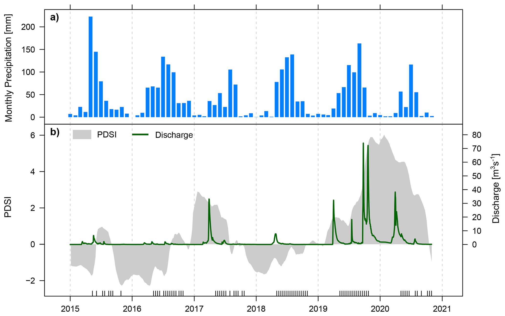
Figure 2 (a) Monthly precipitation sums at Jamestown Regional Airport (from Global Surface Summary of the Day, GSOD; © National Climatic Data Center, NESDIS, NOAA, U.S. Department of Commerce); (b) daily runoff at Pingree (© USGS) and the GRIDMET-derived PDSI (Abatzoglou, 2013) during the observation period. The rug plot at the bottom marks the dates of the Sentinel-1 acquisitions used in this study.

2.2 Data and preprocessing

2.2.1 Sentinel-1 data

Surface water dynamics were derived from a stack of Sentinel-1 interferometric wide swath (IWS) images. Sentinel-1A was launched in April 2014, and its twin satellite Sentinel-1B followed in April 2016. Both satellites carry a C-band SAR instrument operating at a wavelength of ca. 5.6 cm. The ground range detected (GRD) product has a spatial resolution of ca. 20 m (Torres et al., 2012). Data for the study area are available from March 2015 onwards. As wet snow and ice cover on lakes can alter backscatter behaviour, the study was limited to the months from May to October, which we assumed to be mostly snow-free. A total number of 74 scenes acquired between May 2015 and October 2020 were downloaded from the Copernicus Open Access Hub. From 2016, data were available at an interval of 12 d with a few exceptions (Fig. 2b). All of the scenes used in this study were acquired from the same relative orbit (number 34) and were available in both vertical send–vertical receive (VV) and vertical send–horizontal receive (VH) polarisations. The downloaded GRD scenes were filtered using a Gamma-MAP speckle filter (Lopes et al., 1993) with a window size of 3×3 pixels and were radiometrically calibrated to obtain the backscattering coefficient σ⁰. Terrain correction was carried out using the range–Doppler approach and the digital elevation model from the Shuttle Radar Topography Mission (Farr et al., 2007). The scenes were resampled to a common grid with a pixel spacing of 10 m in the Universal Transverse Mercator (UTM Zone 14 North) projection. The SAR data were preprocessed using the Sentinel Application Platform (SNAP version 7), provided by the European Space Agency (ESA).

2.2.2 Topographical data

A digital terrain model (DTM) with a resolution of 1 m was available from the North Dakota State Water Commission (2018) (Fig. 1). The DTM is based on lidar data acquired in autumn 2011. The data package downloaded from the North Dakota GIS Hub also included polygons of waterbodies classified based on the lidar intensity data. For the comparison with Sentinel-1 data, the DTM and the waterbodies were aggregated to the 10 m grid mentioned above. The waterbody polygons were aggregated by retaining pixels as water pixels if they were more than 50 % covered by a water polygon. The height above nearest drainage (HAND), z_HAND, was then computed from the DTM. HAND is defined as the difference in elevation between a given DTM cell and the nearest cell pertaining to the drainage network (Rennó et al., 2008). For this purpose, the flow direction was determined using the D8 (deterministic eight-node) method. The algorithm then follows the flow direction raster until reaching a cell pertaining to the drainage network and computes the height difference between the drainage cell and the original starting cell. The HAND index has been used in flood remote sensing for masking areas that are not prone to floods (Westerhoff et al., 2013; Schlaffer et al., 2015; Twele et al., 2016). In order to take the special environmental conditions encountered in the PPR into account, we used both the identified potholes as well as the drainage network obtained from the DTM after filling the pothole sinks as drainage pixels. The drainage network was extracted using the “r.watershed” tool in GRASS GIS (GRASS Development Team, 2017).

2.2.3 Land use/land cover

As a source of information on land use/land cover, the U.S. Department of Agriculture (USDA) NASS CDL for North Dakota was downloaded (henceforth referred to as CDL). The CDL for 2015 is based on data from Landsat 8, DEIMOS-1 and UK2 that were acquired during that year. The CDL has a spatial resolution of 30 m and is provided under a Creative Commons licence (USDA National Agricultural Statistics Service Cropland Data Layer, 2015). The CDL was resampled to the same 10 m grid as the Sentinel-1 data using nearest-neighbour resampling. Due to the difference in the spatial resolution between the CDL and Sentinel-1, pixels at the border between water and land areas were masked in order to avoid sampling from mixed pixels. Masking was done in both directions, towards water and land (i.e. a buffer of 20 m along the water–land border was avoided when using the information for sampling from the two different distributions).

2.2.4 Validation data

The surface water extents were validated for three different dates in 2016, 2017 and 2019 using aerial imagery from the National Agriculture Imagery Program (NAIP, U.S. Department of Agriculture, Farm Service Agency). These years were selected to have a representation of dry and wet years. The three NAIP scenes cover different parts of the study area (Fig. 1). False-colour composites of the images are shown in Appendix A (Fig. A1). NAIP imagery has a spatial resolution of 1 m and comprises four bands in the visible and near-infrared (NIR) portions of the electromagnetic spectrum. For validating the water extents derived from Sentinel-1, we sampled points across the extent of the NAIP images and classified them manually into water and non-water classes. Although wetlands occur frequently in the study area, a random sample would likely underrepresent surface water. To account for this class imbalance, a stratified random sampling approach was applied. With the help of the DTM-derived potholes, 200 pixels per class were randomly sampled from potholes and upland areas throughout each of the three NAIP footprints, resulting in 400 reference points for each reference image (shown in Fig. A1). The NIR band was especially useful in identifying areas where vegetation was emerging from water surfaces. We assumed that such conditions would fundamentally impact radar backscatter from these areas. Whenever vegetation was protruding through the water surface around a sampling point, the respective point was classified as non-water, as the proposed approach applies only to open water surfaces.

2.3 Water extent delineation

Calm, open water surfaces typically cause specular reflection of incident microwave radiation. In SAR scenes with an approximately balanced mix of open water and land classes, this phenomenon leads to bimodal grey-value histograms. However, these classes rarely occur at similar proportions within a scene, and, as a result, bimodality of the histogram is not commonly observed. Efforts have been made to balance water and non-water classes by subsampling areas from SAR images where water and land pixels are equally represented (Martinis et al., 2009; Schlaffer et al., 2016; Chini et al., 2017). An example of such an effort is split-based approaches (Martinis et al., 2009; Chini et al., 2017), where image subsets showing a bimodal grey-value distribution are automatically selected from a SAR scene based on a set of predefined criteria. This approach is especially useful if the approximate locations of the waterbodies or flooded areas are not known a priori.

The locations of prairie potholes, however, are governed by the landscape features of the PPR and have been reported to be relatively stable over longer time periods (Bolanos et al., 2016). Therefore, we chose to treat the potholes as the baseline of the study (see box (1) in Fig. 3). The pothole locations were determined based on the waterbodies product contained in the 2011 lidar data. We assumed that this dataset contained more waterbodies than what could be classified from satellite data due to the higher spatial resolution and the fact that the data had been acquired during extremely wet conditions (Wu and Lane, 2017). Therefore, it was regarded as a suitable baseline dataset for monitoring surface water dynamics in as many potholes as possible.

An overview of the water classification workflow is shown in Fig. 3. In contrast to other studies on remote-sensing-based water retrieval, which treat a scene uniformly (i.e. by estimating the statistical distributions of water and non-water classes along with classification thresholds across the entire image), the class-specific backscatter distributions were estimated locally (i.e. for each of the known pothole locations) (box (2) in Fig. 3). The reasoning behind this approach is that backscatter values may vary considerably over large regions over water surfaces, due to wind/semi-submerged vegetation, and over land surfaces, due to variations in soil moisture/wet snow cover/vegetation structure and moisture.

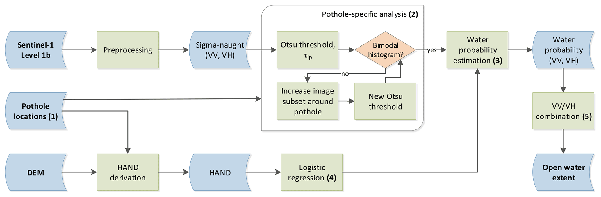
Figure 3 Sentinel-1 processing workflow for dynamic open water classification. Bold numbers in parentheses indicate key datasets and processing steps referred to in the text.

In order to estimate the backscatter distribution expected for open water, an independent reference layer is required (Schlaffer et al., 2017), for example, derived from optical data. Here, we chose the CDL for 2015 (USDA National Agricultural Statistics Service Cropland Data Layer, 2015) as the reference layer. Backscatter values for open waterbodies delineated in the CDL were extracted for the months from May to October, henceforth denoted as ${\mathit{\sigma }}_{\mathrm{w},\mathrm{p}}^{\mathrm{0}}$ for each of the two polarisations p∈{VV,VH}. The mean of ${\mathit{\sigma }}_{\mathrm{w},\mathrm{p}}^{\mathrm{0}}$ is ${\stackrel{\mathrm{‾}}{{\mathit{\sigma }}^{\mathrm{0}}}}_{\mathrm{w},\mathrm{p}}$. For each of the previously delineated potholes, we checked if at least 10 pixels had ${\mathit{\sigma }}_{\mathrm{p}}^{\mathrm{0}}$ values lower than ${\stackrel{\mathrm{‾}}{{\mathit{\sigma }}^{\mathrm{0}}}}_{\mathrm{w},\mathrm{p}}$. If this condition was not fulfilled, it was assumed that no open water was present in the respective pothole. Otherwise, we proceeded to check the bimodality of the backscatter distribution within the pothole. We followed the approach by Chini et al. (2017) for this. As a first guess, the histogram was automatically split using the Otsu approach (Otsu, 1979). This initial threshold for polarisation p is referred to as τ_ip in the following. The bimodality was then assessed using Ashman’s D (Ashman et al., 1994), which is defined as

$$\begin{array}{}\text{(1)}& D=\sqrt{\mathrm{2}}{\displaystyle \frac{|{\mathit{\mu }}_{\mathrm{1}}-{\mathit{\mu }}_{\mathrm{2}}|}{{\mathit{\sigma }}_{\mathrm{1}}^{\mathrm{2}}+{\mathit{\sigma }}_{\mathrm{2}}^{\mathrm{2}}}},\end{array}$$

where μ₁ and ${\mathit{\sigma }}_{\mathrm{1}}^{\mathrm{2}}$ are the mean and variance of all ${\mathit{\sigma }}_{\mathrm{p}}^{\mathrm{0}}\le {\mathit{\tau }}_{\mathrm{ip}}$ respectively, and μ₂ and ${\mathit{\sigma }}_{\mathrm{2}}^{\mathrm{2}}$ are the mean and variance of all ${\mathit{\sigma }}_{\mathrm{p}}^{\mathrm{0}}>{\mathit{\tau }}_{\mathrm{ip}}$ respectively. A value of D>3 was assumed to be an indication of a bimodal histogram. If this condition was not fulfilled, the region around the pothole was extended to include neighbouring pixels in order to include a higher number of non-water pixels and was then checked again for bimodality. For each pothole, the sampling region around the pothole was further extended by including neighbouring pixels up to a maximum number of 10 iterations. If a bimodal histogram was encountered before reaching this number of iterations, the final Otsu threshold for the respective pothole was saved. In the following, the threshold value derived for ${\mathit{\sigma }}_{\mathrm{p}}^{\mathrm{0}}$ is denoted as τ_p. In processing step (3) shown in Fig. 3, the parameters of the respective backscatter distributions for water (w) and land (l) for each pothole were estimated as

$$\begin{array}{}\text{(2)}& {\mathit{\mu }}_{\mathrm{w},\mathrm{p}}=\sum {\mathit{\sigma }}_{\mathrm{w},\mathrm{p}}^{\mathrm{0}}/N_{\mathrm{w},\mathrm{p}},{\mathit{\sigma }}_{\mathrm{w},\mathrm{p}}^{\mathrm{2}}={\displaystyle \frac{\mathrm{1}}{N_{\mathrm{w},\mathrm{p}}-\mathrm{1}}}\sum {\mathit{\sigma }}_{\mathrm{w},\mathrm{p}}^{\mathrm{0}},\end{array}$$

and

$$\begin{array}{}\text{(3)}& {\mathit{\mu }}_{\mathrm{l},\mathrm{p}}=\sum {\mathit{\sigma }}_{\mathrm{l},\mathrm{p}}^{\mathrm{0}}/N_{\mathrm{l},\mathrm{p}},{\mathit{\sigma }}_{\mathrm{l},\mathrm{p}}^{\mathrm{2}}={\displaystyle \frac{\mathrm{1}}{N_{\mathrm{l},\mathrm{p}}-\mathrm{1}}}\sum {\mathit{\sigma }}_{\mathrm{l},\mathrm{p}}^{\mathrm{0}}.\end{array}$$

Here, ${\mathit{\sigma }}_{\mathrm{w},\mathrm{p}}^{\mathrm{0}}$ values are all ${\mathit{\sigma }}_{\mathrm{p}}^{\mathrm{0}}\le {\mathit{\tau }}_{\mathrm{p}}$, and ${\mathit{\sigma }}_{\mathrm{l},\mathrm{p}}^{\mathrm{0}}$ values are all ${\mathit{\sigma }}_{\mathrm{p}}^{\mathrm{0}}>{\mathit{\tau }}_{\mathrm{p}}$. N_w, p and N_l, p are the number of ${\mathit{\sigma }}_{\mathrm{w},\mathrm{p}}^{\mathrm{0}}$ and ${\mathit{\sigma }}_{\mathrm{l},\mathrm{p}}^{\mathrm{0}}$ values respectively. The probability of a pixel belonging to the water distribution given a certain value of ${\mathit{\sigma }}_{\mathrm{p}}^{\mathrm{0}}$ was computed as

$$\begin{array}{}\text{(4)}& p\left(W\right|{\mathit{\sigma }}_{\mathrm{p}}^{\mathrm{0}})={\displaystyle \frac{p\left({\mathit{\sigma }}_{\mathrm{p}}^{\mathrm{0}}\right|W\left)p\right(W)}{p\left({\mathit{\sigma }}_{\mathrm{p}}^{\mathrm{0}}\right|W\left)p\right(W)+p({\mathit{\sigma }}_{\mathrm{p}}^{\mathrm{0}}\left|L\right)[\mathrm{1}-p(W\left)\right]}}.\end{array}$$

$p\left({\mathit{\sigma }}_{\mathrm{p}}^{\mathrm{0}}\right|W)$ and $p\left({\mathit{\sigma }}_{\mathrm{p}}^{\mathrm{0}}\right|L)$ are the probability density functions (PDFs)

$$\begin{array}{}\text{(5)}& p\left({\mathit{\sigma }}_{\mathrm{p}}^{\mathrm{0}}\right|W)={\displaystyle \frac{\mathrm{1}}{\sqrt{\mathrm{2}\mathit{\pi }{\mathit{\sigma }}_{\mathrm{w},\mathrm{p}}^{\mathrm{2}}}}}{e}^{\frac{{\mathit{\sigma }}_{\mathrm{p}}^{\mathrm{0}}-{\mathit{\mu }}_{\mathrm{w},\mathrm{p}}}{\mathrm{2}{\mathit{\sigma }}_{\mathrm{w},\mathrm{p}}^{\mathrm{2}}}}\end{array}$$

and

$$\begin{array}{}\text{(6)}& p\left({\mathit{\sigma }}_{\mathrm{p}}^{\mathrm{0}}\right|L)={\displaystyle \frac{\mathrm{1}}{\sqrt{\mathrm{2}\mathit{\pi }{\mathit{\sigma }}_{\mathrm{l},\mathrm{p}}^{\mathrm{2}}}}}{e}^{\frac{{\mathit{\sigma }}_{\mathrm{p}}^{\mathrm{0}}-{\mathit{\mu }}_{\mathrm{l},\mathrm{p}}}{\mathrm{2}{\mathit{\sigma }}_{\mathrm{l},\mathrm{p}}^{\mathrm{2}}}}.\end{array}$$

The p(W) term in Eq. (4) denotes the prior probability of a pixel being land or water. If no information is available, p(W)=0.5 can be used to give equal prior probability to the land and water distributions (Giustarini et al., 2016). However, as the location of the open water surfaces was known to be mainly confined by the topography of the potholes, which changes little over time (Bolanos et al., 2016), we chose to incorporate this knowledge. Bayes’ theorem has been used as an efficient framework to fuse information from different sources, for example, for obtaining SAR-based flood delineation maps (e.g. Frey et al., 2012; D'Addabbo et al., 2016; Li et al., 2019). Here, p(W) was modelled using a logistic regression with z_HAND as the predictor (step (4) in Fig. 3):

$$\begin{array}{}\text{(7)}& p\left(W\right)={\displaystyle \frac{\mathrm{1}}{\mathrm{1}+e^{-b_{\mathrm{0}}-b_{\mathrm{1}}{z}_{\text{HAND}}}}},\end{array}$$

where b₀ and b₁ are regression parameters which were estimated using 20 samples, each consisting of 5000 land and 5000 water pixels identified from the CDL. An additional sample of 4985 land and 4668 water pixels not containing any of the pixels used for training was set aside for testing. When sampling the training and testing data, pixels in a buffer region along the border between land and water were excluded to obtain a pure sample of each class. Pixels that are identified as land in the CDL may still be prone to the occurrence of wetlands. For example, they may be located in depressions that have been drained or may not have been covered by water when the imagery used for the CDL was acquired. In order to account for potential sampling biases, Eq. (7) was fitted to each of the 20 training samples separately, and the average of the estimated parameters b_0, i and b_1, i, where $\mathrm{0}<\mathrm{i}\le \mathrm{20}$, was used to estimate p(W).

The estimated $p\left(W\right|{\mathit{\sigma }}_{\mathrm{p}}^{\mathrm{0}})$ values were classified into water and non-water classes considering the spatial relationship between areas with high $p\left(W\right|{\mathit{\sigma }}_{\mathrm{p}}^{\mathrm{0}})$, which changes over time, and the static pothole extents derived from the DTM. This approach served to minimise the occurrence of isolated clusters of water pixels far from potholes which may occur due to speckle or dry land surfaces appearing as dark areas in the SAR image. This condition was implemented using a region-growing approach with the DTM-based pothole area as seed. The region growing was limited to a maximum of 10 iterations to prevent “spilling” of positive pixels into large portions of the scene. The idea is illustrated in Fig. 4. Two potholes are separated in the DTM by a low topographic barrier (left). However, the potholes are visibly merged together in the Sentinel-1 image shown in the centre. After the region growing, the classification result shows the merged waterbodies (right).

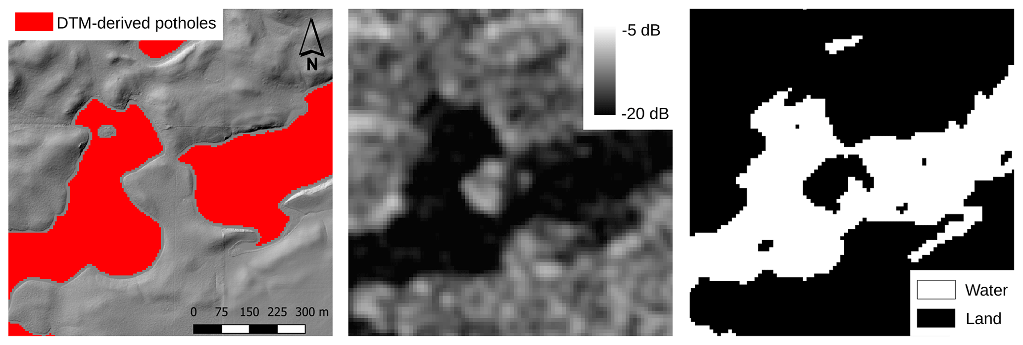
Figure 4 The left panel shows the DTM hillshade and derived potholes, the middle panel displays the Sentinel-1 ${\mathit{\sigma }}_{\text{VV}}^{\mathrm{0}}$ on 31 May 2017, and the right panel outlines the derived open water extent.

In addition, the final water area should take the information from both VV and VH polarisations into account. The respective water probabilities, $p\left(W\right|{\mathit{\sigma }}_{\text{VV}}^{\mathrm{0}})$ and $p\left(W\right|{\mathit{\sigma }}_{\text{VH}}^{\mathrm{0}})$, were combined based on their values (step (5) in Fig. 3). We opted for a rather conservative approach for combining the two datasets to minimise the occurrence of false positives. In summary, we applied the following conditions for classifying dynamic open water from water probability:

• i

  $p\left(W\right|{\mathit{\sigma }}_{\text{VV}}^{\mathrm{0}})>\mathrm{0.8}\vee p(W\left|{\mathit{\sigma }}_{\text{VH}}^{\mathrm{0}}\right)>\mathrm{0.8}\vee \left[p\right(W\left|{\mathit{\sigma }}_{\text{VV}}^{\mathrm{0}}\right)>\mathrm{0.5}\wedge p\left(W\right|{\mathit{\sigma }}_{\text{VH}}^{\mathrm{0}})>\mathrm{0.5}]$, where ∨ is a logical OR, and ∧ is a logical AND;

• ii

  there is a ≤10 pixel distance to the original pothole area;

• iii

  the derived water area is connected with the original pothole area (taking all eight neighbours of each pixel into account).

For validation, producer’s and user’s accuracies were computed for the water class using the combined product against the reference data described in Sect. 2.2.4. Each of the three reference datasets was compared to the Sentinel-1-derived waterbodies closest in time to the date of the respective NAIP acquisition. In order to estimate the impact of using VV or VH polarisation, accuracies were also computed for each polarisation separately using a threshold of $p\left(W\right|{\mathit{\sigma }}_{\mathrm{p}}^{\mathrm{0}})>\mathrm{0.5}$.

2.4 Analysis of surface water dynamics

Prairie wetlands can merge over time with neighbouring wetlands or split into separate waterbodies. Hence, monitoring the area of individual waterbodies is challenging. To track surface water dynamics across the study area, we computed the total water area, areas covered by individual waterbodies and the number of waterbodies for each of the observation dates. Furthermore, we were interested in the inter- and intra-annual dynamics of wetlands of different sizes. For this purpose, waterbodies were divided in four different size bins, and the contribution of each bin to the total water extent was tracked along the observation period. The metrics were computed using the “landscapemetrics” R package (Hesselbarth et al., 2019). In accordance with the spatial resolution of the Sentinel-1 sensor, before deriving the metrics we applied a minimum mapping unit of 0.04 ha, equal to the area of four pixels, to remove small clusters of water pixels from the result. Such small clusters are often the result of noise. For easier visual interpretation, the obtained time series were further smoothed by overlaying a locally estimated scatterplot smoothing (LOESS; Cleveland et al., 1992) taking the observations of the current year into account.

3 Results and discussion

3.1 Open water classification

The obtained p(W) values are shown in Fig. 5. It can be seen that high p(W) predominantly occur in potholes and along rivers and streams, whereas most of the upland areas are assigned values close to zero. We validated the estimated p(W) using an independent test sample with labels assigned from the lidar-based water map. Calculating an overall accuracy for the test sample would not take the unknown occurrence of potential wetlands in the CDL land class into account. Therefore, we computed the sensitivity of our approach as $s=\mathrm{TP}/(\mathrm{TP}+\mathrm{FN})$, where TP denotes true positives, and FN denotes false negatives, after classifying the predicted p(W) into binary values using a threshold of p(W)=0.5. The sensitivity quantifies the capability of the classifier to correctly identify existing waterbodies and was calculated as s=0.985.

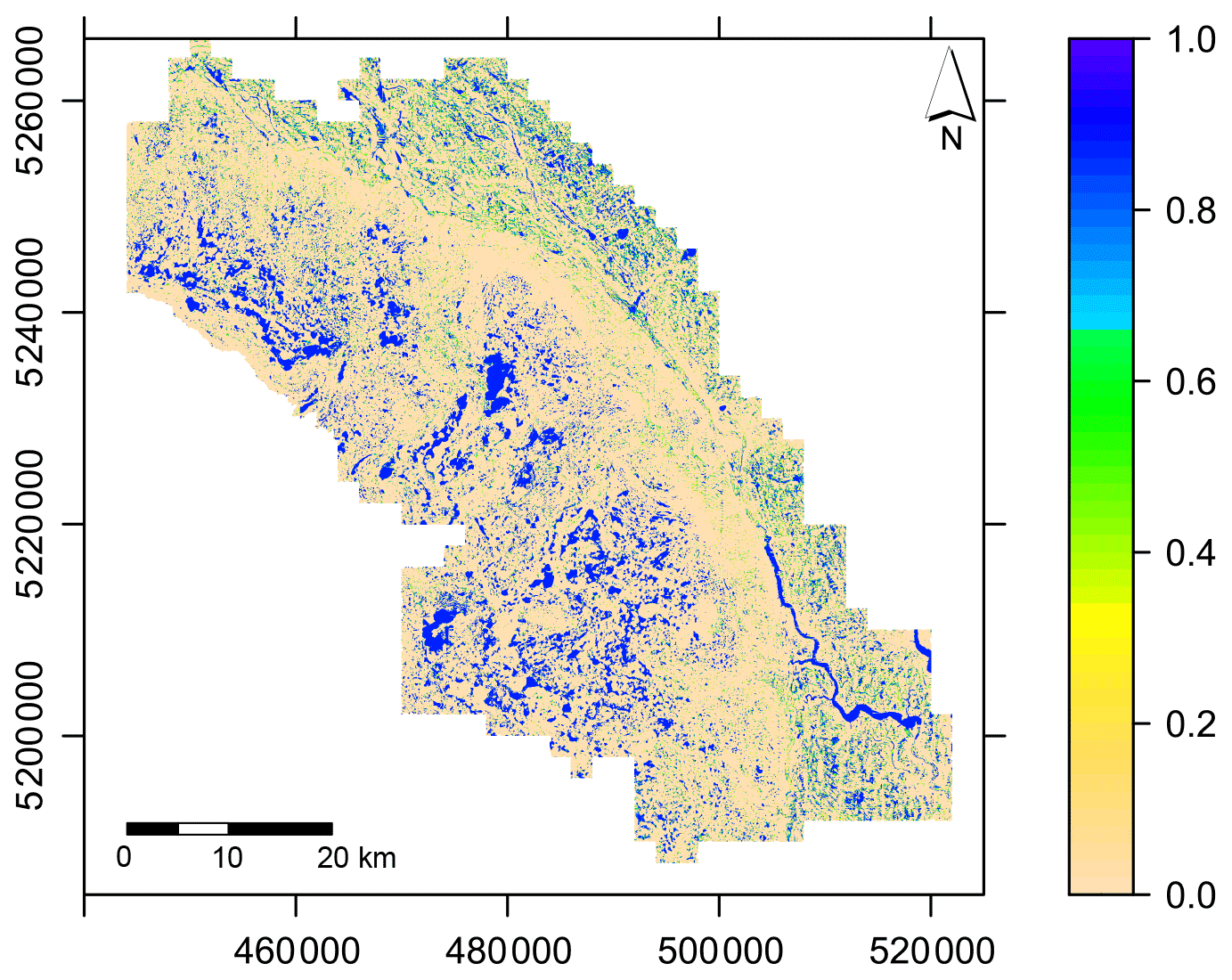
Figure 5 Map of prior water probabilities p(W) predicted from Eq. (7) with b₀=1.9479 and $b_{\mathrm{1}}=-\mathrm{3.5598}$. Scales show coordinates in the Universal Transverse Mercator system (UTM zone 14).

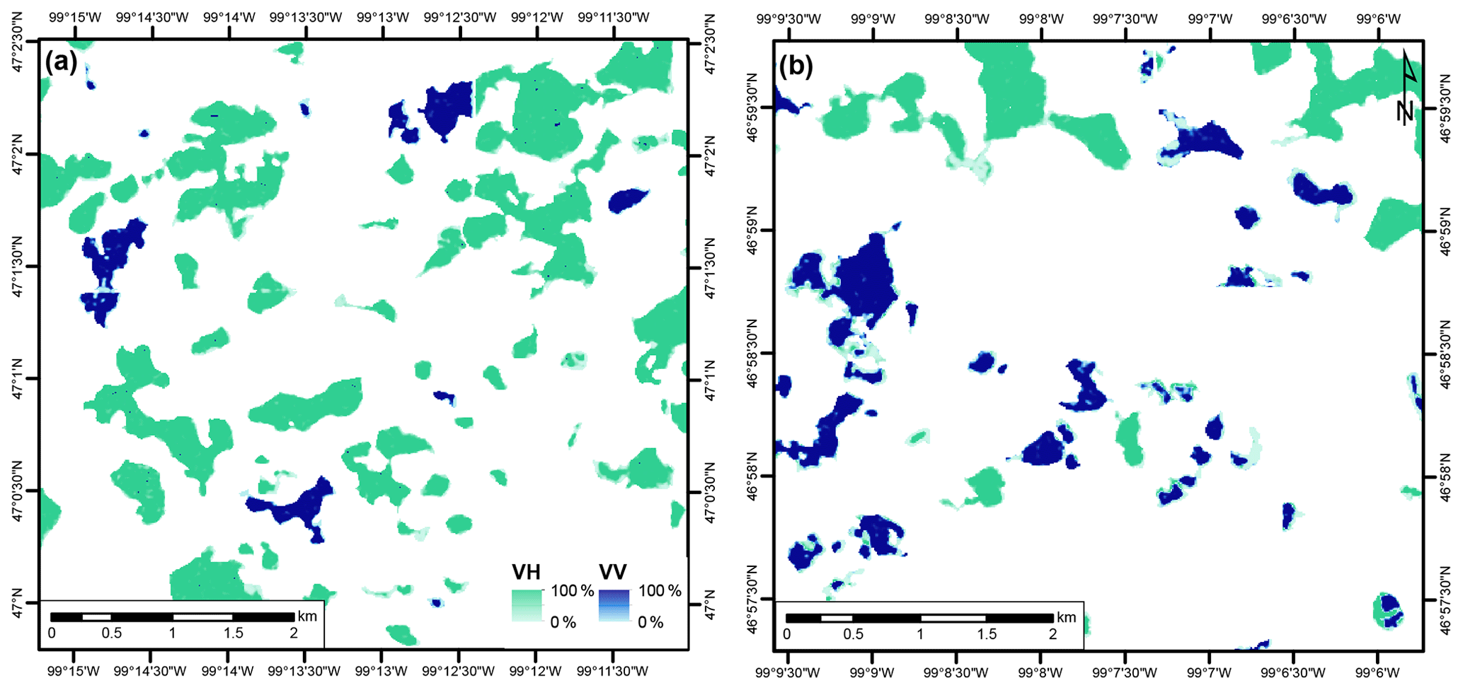
Open water maps were produced for the months from May to October for the period from 2015 to 2020 (Fig. 6c, d). In Fig. 6c, most of the waterbodies were identified in both VV and VH polarisations. However, the subset also shows several wetlands only detected in VV, visible as light-blue areas in the RGB composite. VH backscatter over land areas is mainly related to volume scattering. In areas with sparse vegetation density, this may lead to a low contrast between water and non-water in the VH band of the image. In such cases, no suitable threshold could be determined. The subset shown in Fig. 6d contains several wetlands only classified in the VH data (pink colour). Comparison with the corresponding backscatter image (Fig. 6b) reveals that VV backscatter seems to be increased over these waterbodies, as indicated by the reddish colours. This, in turn, leads to lower contrast between water and surrounding non-water classes. In some cases, waterbodies could not be detected in either polarisation, such as the large waterbody in the centre of Fig. 6d and f. This is often the case when either ice cover is present/the water surface is roughened by wind or when the surrounding land surface appears dark, as in the centre of Fig. 6b. Such darker areas are often related to grassland and sparsely vegetated areas, which can be distinguished in the false-colour images in Fig. 6e and f by their paler appearance compared with vegetated fields (visible in bright red). Agricultural fields tend to appear brighter in the SAR imagery (Fig. 6a, b) owing to high soil moisture and vegetation influencing both VV- and VH-polarised backscatter.

Figure 6 Panels (a) and (b) show colour composites of ${\mathit{\sigma }}_{\text{VV}}^{\mathrm{0}}$ (red) and ${\mathit{\sigma }}_{\text{VH}}^{\mathrm{0}}$ (green) on 5 July 2016, panels (c) and (d) present classification results as RGB composites (R – VH; G – VV; and B – final classification, Fin); and panels (e) and (f) display false-colour composites (R – near-infrared, G – red and B – green) of NAIP imagery acquired on 4 July 2016.

Comparison with independent NAIP data, which was carried out for three dates, resulted in high producer’s accuracies (>84 %) for two dates and very high user’s accuracies for all three dates (>98 %), suggesting some underestimation of the water extent (Table 1). The high user’s accuracies are the result of a very low number of false positives. The underestimation of the water extent is to be expected due to the difference in spatial resolution between Sentinel-1 (ca. 20 m) and the reference data (1 m). In such cases, validation points located close to the edges of objects may coincide with mixed pixels in the lower-resolution imagery. In the case of the validation carried out for July 2016, producer’s accuracies were lower, especially for VV, possibly due to wind roughening the water surface. Such effects are visible in the NAIP imagery and may have also occurred on the following day when the Sentinel-1 scene was acquired. The extent of the NAIP image acquired in 2019 is located in the upper Pipestem catchment and dominated by a high number of small waterbodies that were sometimes not detected by our approach, leading to somewhat lower producer’s accuracies (below 90 %).

Table 1 Accuracy values of open water classification for three dates.

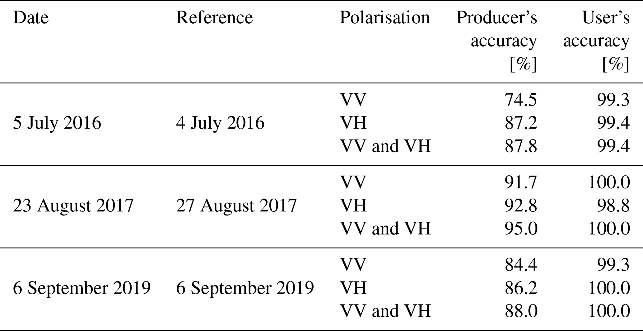
The accuracies reported here are similar to the ones reported by Huang et al. (2018), who compared the open water extent derived from dual-polarised Sentinel-1 data against reference extents derived from NAIP imagery over the Pipestem Basin. The authors of that study also used the scene acquired on 5 July 2016 for validation. For the water class, they obtained producer’s accuracies between 64 % and 92 % and user’s accuracies between 87 % and 99 %. For the wind-affected scene of July 2016, a producer’s accuracy of 64 % was reported, whereas a producer’s accuracy of 87.8 % was obtained here with the combination of VV and VH polarisations. The inclusion of topographic information may have helped to mitigate the effect of the backscatter increase due to the wind-roughened water surface. This interpretation is supported by the relatively high producer’s accuracy of 74.5 % for VV on that day. In comparison to Huang et al. (2018), user’s accuracies reported here were consistently higher, suggesting a lower overestimation of water extent. We attribute this to the integration of HAND in the Bayesian framework, which helped to constrain water extent retrieval even in image areas where the contrast between water and non-water pixels was low. Such low-contrast areas often lead to a “spilling” into non-water areas during the region-growing process.

Wind is an important environmental factor in the prairies and has been shown to affect SAR water extent retrieval by causing scattering from roughened water surfaces (Bartsch et al., 2012). As a result, the contrast between water and non-water areas may be decreased to the point that no distinction is possible, even by visual means. Such a case can be observed in Fig. 7a, where hardly any open water surfaces could be detected by the algorithm. The scene was acquired on a windy day during which average wind speed measured at nearby Jamestown Regional Airport exceeded the 99 % quantile of the recorded daily averages since 1990 (source: GSOD). Especially larger waterbodies are not visible in the co-polarised backscatter image due to the low contrast. The waterbody delineation based on VH-polarised data, however, did not display the same issues. While the backscatter from larger open waterbodies still shows some influence of water surface roughening, this fact inhibited water extent delineation to a far lower degree (Fig. 7b).

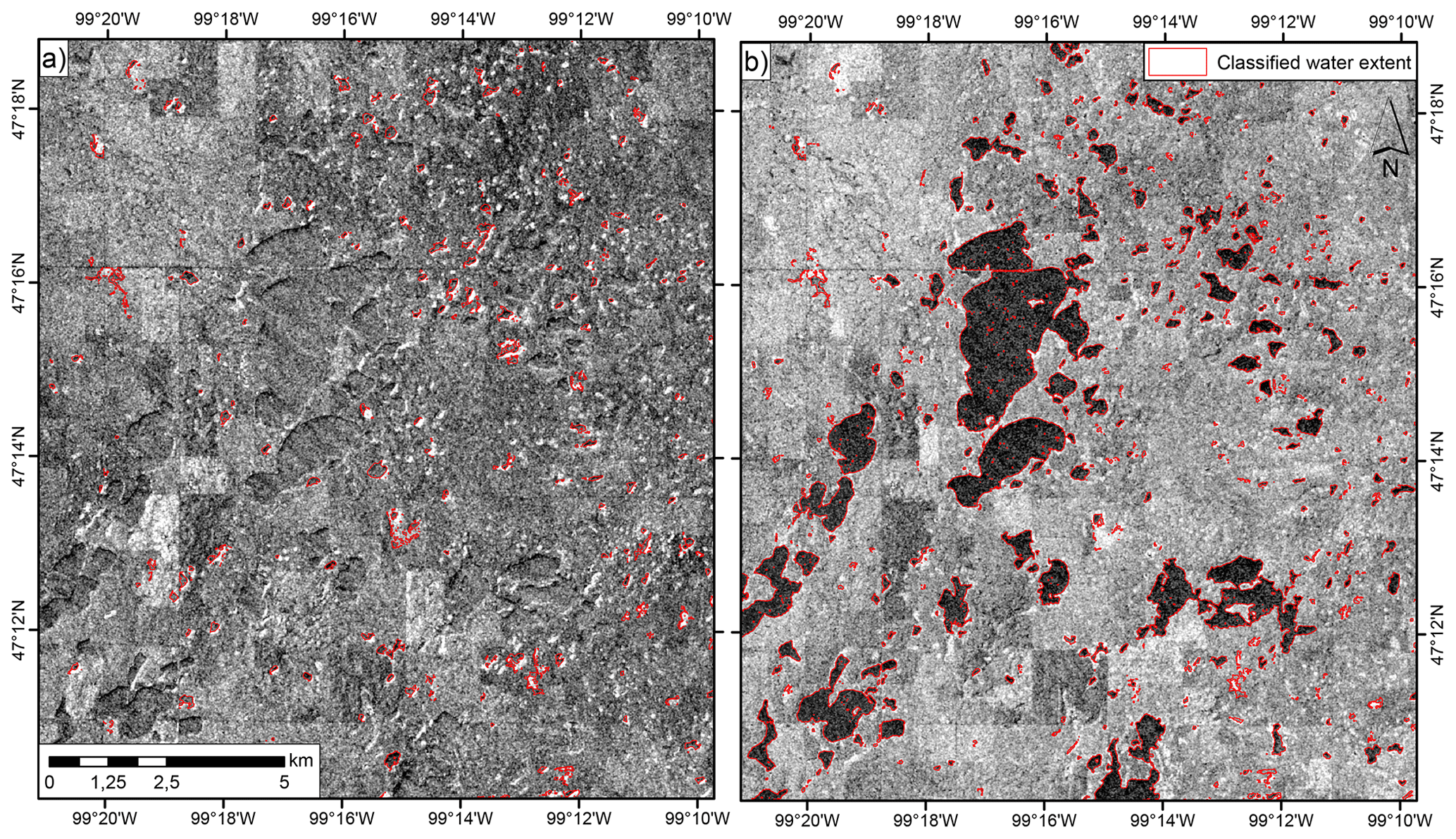
Figure 7 Backscatter in (a) VV and (b) VH polarisation as well as derived waterbodies on 12 October 2019.

The effect of wind on SAR backscatter from water surfaces was a frequently encountered problem in this study, especially for VV-polarised imagery. VH data were shown to be less affected by this problem, which is in line with our expectations and findings available in the literature (Henry et al., 2006). However, as the cross-polarised signal is dominated by volume scattering (Richards, 2009), areas with sparse vegetation often resemble water surfaces in the resulting imagery (Twele et al., 2016). Hence, its full potential lies in its complementary use with co-polarised data, as was demonstrated here.

Overall, the proposed approach for water extent classification represents an efficient way of fusing SAR backscatter with topographical information via the derivation of HAND. Such probabilistic approaches have drawn some attention in recent years to combine SAR imagery with multi-temporal and ancillary sources of information (D'Addabbo et al., 2016; Li et al., 2019). D'Addabbo et al. (2016) used interferometric coherence, a geomorphic flood index and Euclidean distance from a river to incorporate a priori information on the probability of an area becoming flooded during an inundation event. The authors note that, when using the ancillary information, both false and missed alarms were reduced with respect to the use of SAR intensity data only. Furthermore, the probabilistic information obtained using the Bayesian approach may add some information on the uncertainty of the produced maps. The intermediate probabilistic maps (Fig. B1) corresponding to the images shown in Fig. 6 show rather crisp borders between areas with low and high water probability. There are, however, some areas with intermediate $p\left(W\right|{\mathit{\sigma }}_{\mathrm{p}}^{\mathrm{0}})$ values, mainly between high-probability wetlands. It should be noted that, in this study, fixed thresholds were used to convert the continuous probabilistic maps into binary water maps combining both VV and VH polarisations. However, receiver operating characteristic curves may be used to select more optimal thresholds by balancing true and false positive rates.

3.2 Surface water dynamics

Throughout the study period, the number of potholes with open water surfaces strongly varied between ca. 2300 and more than 5000. The total water surface area varied between ca. 14 000 ha and more than 18 000 ha (Fig. 8). A number of outliers occur in the time series. For example, the image acquired on 12 October 2019, when heavy winds influenced the water retrieval (Fig. 7), has a lower number of waterbodies, a lower total water area and a higher average water area per detected waterbody, indicating that only larger objects could be detected. In addition, for example, in October of the years 2015, 2017, 2018 and 2020, the number of waterbodies and their median area showed sudden changes due to wind on the water surface or emerging ice cover which limited the algorithm’s capability to accurately delineate the surface water extent. As a result, large waterbodies were only partially classified as water and, therefore, higher numbers of small waterbodies were erroneously identified. In the following, the results for these dates will not be taken into account.

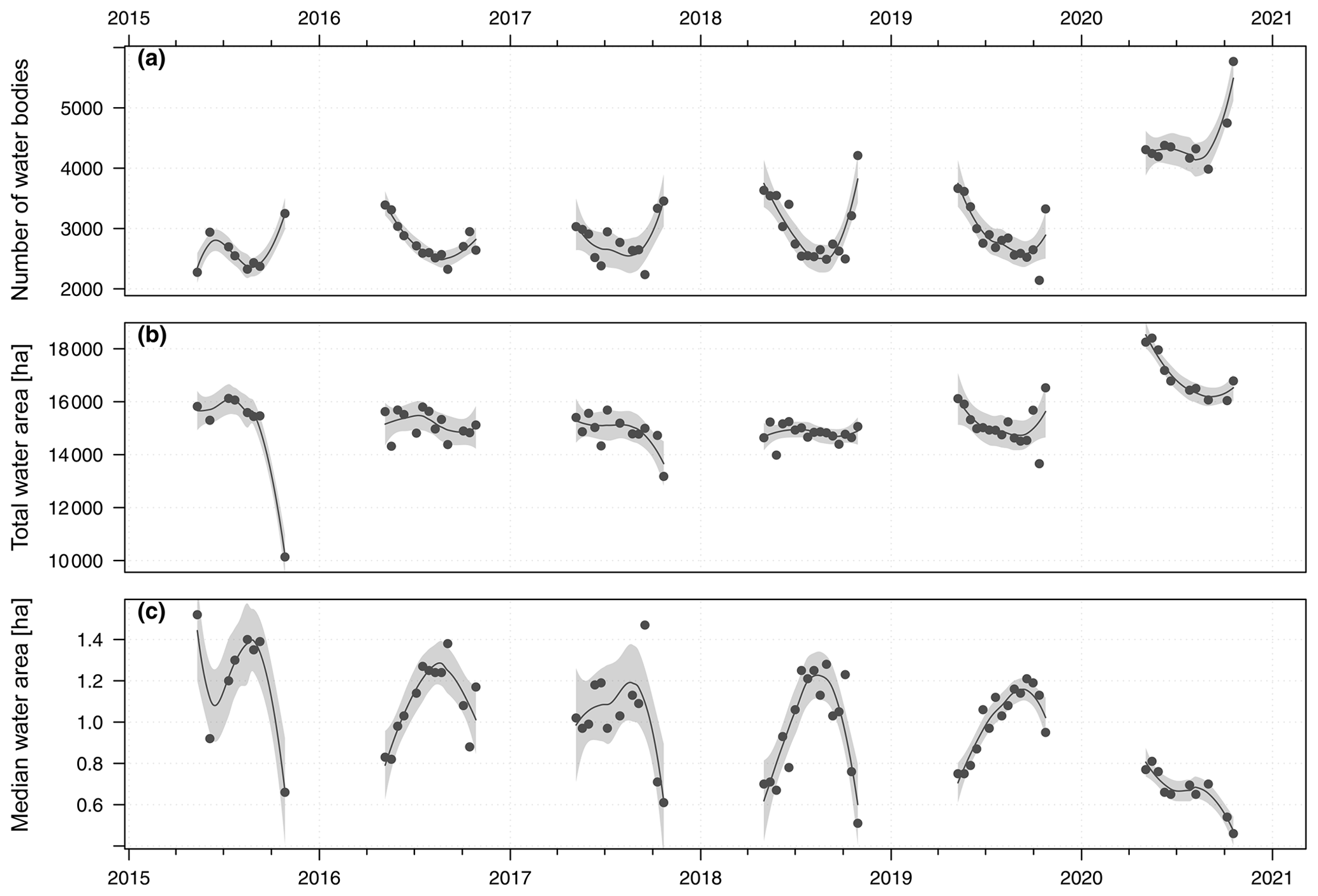
Figure 8 (a) Number of waterbodies, (b) total water area and (c) median waterbody size across the Pipestem Creek basin for each of the Sentinel-1 scenes. Lines show LOESS smoothing functions along with 95 % confidence intervals.

We first report and discuss seasonality in the derived observed water area, number of waterbodies and average area per waterbody. Subsequently, inter-annual differences are reported and discussed in the context of ancillary hydrometeorological information.

3.2.1 Intra-annual surface water dynamics

In most years, the number of waterbodies and total water area displayed a seasonal behaviour: the highest numbers are observed in spring, there is an annual minimum in late summer, and the numbers increase again during September and October (Fig. 8a, b). The decline in water area from spring throughout summer was especially noticeable in 2017, when water area decreased from ca. 15 400 ha in May to ca. 13 180 ha in October (Fig. 8b). The median area per waterbody (Fig. 8c) was similar to the inverse of the number of waterbodies. Potholes tended to have larger water areas in summer than in spring and autumn. In combination with the seasonal decrease in water area and number of waterbodies, this suggests that smaller waterbodies dry out during summer. Further evidence for this assumption is found when looking at the contribution of different waterbody size classes to the total water area during the study period (Fig. 9). In the following, waterbodies >1 ha will be referred to as large waterbodies, and waterbodies <1 ha will be referred to as small waterbodies. Large waterbodies accounted for most of the total water area in the Pipestem Basin. The water area in these size classes (1–8 ha and >8 ha), with the exception of the aforementioned dates affected by wind and ice cover, was rather stable until 2018 and showed little seasonal variability (Fig. 9a, b). The water area accounted for by small waterbodies, however, showed a clear seasonal pattern with a decrease in water area from spring throughout summer (Fig. 9c, d).

In general, the temporal patterns found in these variables followed the expected seasonality. In a modelling study, Liu and Schwartz (2011) reported intra-annual dynamics with the number of small waterbodies declining from spring throughout summer, whereas the number of larger waterbodies remained stable throughout the year. Our results, covering a period of 6 years, corroborate these findings. In most years, the contribution of small waterbodies to total water extent declined from May towards the end of summer and then increased again until the end of October. The area of larger waterbodies, however, remained stable. Along with the typical seasonal decline in the number of waterbodies and the increase in median waterbody size, this suggests that a large number of small waterbodies fall dry during the summer months when evaporation rates are high. In the following year, these small potholes typically refill after spring rains and snowmelt.

Figure 9 Summed areas of waterbodies in size classes (a) >8 ha, (b) 1–8 ha, (c) 0.2–1 ha and (d) 0.05–0.2 ha. Lines show LOESS smoothing functions along with 95 % confidence intervals.

3.2.2 Inter-annual surface water dynamics

In general, the number of waterbodies, the total water area and the median area per waterbody were relatively stable between 2015 and 2019, whereas 2020 differed considerably from the rest of the observation period in terms of these three metrics (Fig. 8). Between 2015 and 2019, the total water area varied between ca. 14 000 and 16 000 ha. In the first half of the study period, total water area declined from ca. 16 000 ha in 2015 to 15 000 ha in 2017. During 2018, total water area remained stable. In contrast, 2019 started with higher values which then declined by ca. 1500 ha until mid-September. This was followed by a steep increase until the water area reached its maximum of the study period up to that point at ca. 16 500 ha (Fig. 8b). This increase coincides with the exceptional spring floods of that year and the wet October leading to widespread flooding along the James River and other regions of ND (Umphlett, 2019). In addition to the strong increase in total water area at the end of 2019, which is not found in other years, a decrease in median water area per pothole (Fig. 8c) and a larger number of waterbodies (Fig. 8a) can be observed, suggesting that a large number of small potholes filled due to the intense storm event. Both in spring and during the storm event in October 2019, water area was higher than in summer in all four wetland size classes (Fig. 9). Large waterbodies accounted for 88.7 % of the total increase in water area of almost 2000 ha between 18 September and 24 October 2019. The year 2020 differed from the rest of the study period with respect to all three indicators shown in Fig. 8. The number of waterbodies and the total water area were consistently higher than in all previous years, with both indicators surpassing the maximum values of those years during all of the observed months in 2020. At the same time, the median area per waterbody was smaller in 2020 than in previous years, indicating a much larger abundance of small waterbodies. The decrease in both total water area and the median area along with the stable or even increasing number of waterbodies suggests that small waterbodies remained present throughout 2020. The persistence of small waterbodies throughout 2020 becomes obvious when looking at the contributions of waterbodies of different sizes to the total water area (Fig. 9). During that year, large waterbodies showed inverse behaviour compared with small waterbodies: while the water area in the larger two size classes declined between May and July, the total area of small waterbodies stayed relatively stable and increased in autumn.

The strong increase in water area and the emergence of small wetlands in October 2019 with respect to an earlier year can also be observed in the water extent maps in Fig. 10. In 2016 (Fig. 10a, b), a decrease in the extent of waterbodies is visible from early summer (green colour) towards August (dark blue and yellow). The decreased water extent led to a disconnection of some wetlands into several smaller waterbodies. Between August and October, water extent only increased by a small amount, which can be seen in red. During 2019, in contrast, the open water extent visible in June (green colour) was small, whereas in later months, August and October (orange and red colour respectively), the water extent increased and, especially in October, many wetlands began to merge (Fig. 10c, d). This disconnecting and merging behaviour illustrates that an increase in overall water area does not necessarily translate into an increase in the number of small waterbodies (and vice versa). This may explain some of the seemingly different temporal patterns seen in total water area, number of waterbodies and median waterbody size in Fig. 8. At the time of writing, we could not find an analysis of the effects of the 2019 extreme events on wetland extents in the literature. While extensive floods have been reported for spring 2019 across the Midwest (Umphlett, 2019; NOAA, 2019), which are visible as peaks in the discharge time series, the autumn event led to much higher flood peaks in the Pipestem Creek (Fig. 2). The merging of smaller wetlands into larger ones reported here may contribute to this behaviour. This finding may suggest that larger, connected, waterbodies contributed more to floodwater runoff than small, isolated waterbodies.

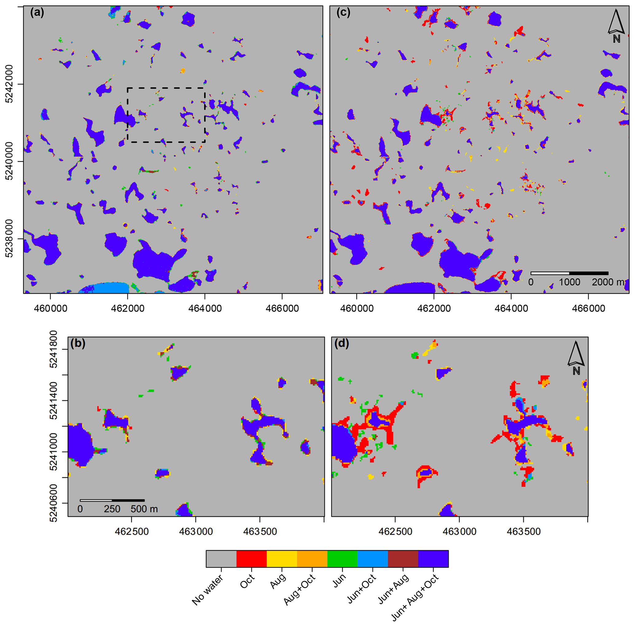
Figure 10 Water extent dynamics in (a, b) 2016 and (c, d) 2019 in a subset of the study area. Observation times refer to 5 July 2016 and 14 June 2019, 10 August 2016 and 13 August 2019, and 27 October 2016 and 24 October 2019 respectively. The “+” symbol denotes water detected at multiple observation times. Dark blue areas were detected as water on all three dates. The box in panel (a) marks the extent of the detailed maps shown in panels (b) and (d). Scales show coordinates in the Universal Transverse Mercator system (UTM zone 14).

To our knowledge, this study is the first time that surface water dynamics in the PPR have been monitored using Sentinel-1 over an extended period covering both dry and wet years. This enables us to also support findings from previous studies (e.g. Liu and Schwartz, 2011) on inter-annual differences in wetland extent. While intra-annual changes in water extent have been found mainly for small waterbodies, larger wetlands should only change on an inter-annual timescale. Our results demonstrate that the contribution of wetlands both larger and smaller than 1 ha to the total water extent is in line with what would be expected from meteorological indices indicating water availability, such as the PDSI (Fig. 2). During the extremely wet period in late 2019–early 2020, large waterbodies showed significantly higher water extent values than during the rest of the study period. It is noteworthy that these increased water extents in larger wetlands decreased again relatively quickly along with the decrease in the PDSI during 2020, whereas the extent of small waterbodies remained relatively stable. This may suggest that larger wetlands can act as a water reservoir during wet periods but then return to their formerly stable extent by releasing water to the drainage network. Small potholes, however, tend to be more geographically isolated – that is to say, they do not have well-defined inlets or outlets and their water balance is mainly controlled by vertical fluxes, such as rainfall, evaporation and drainage to the subsoil (Cohen et al., 2016). They may persist as long as meteorological conditions are wet enough to support them. During most of 2020, the PDSI was above 2 in the study region, which indicates such conditions. Furthermore, the snowpack during the winter of 2019–2020 was thicker than normal (Umphlett, 2019), and the water released after melting fed many of the smaller potholes, also leading to a higher number of smaller waterbodies.

Inter-annual changes in prairie wetland extent have been tracked using Landsat data (Vanderhoof et al., 2016; Krapu et al., 2018; Rover et al., 2011) and high-resolution aerial imagery (Wu and Lane, 2017; Wu et al., 2019); however, the limitations due to cloud cover and the long intervals between the acquisition of NAIP data typically do not allow for the reproduction of extreme events. The analysis of SAR time series unaffected by cloud cover and with high temporal resolution may help to understand the complex threshold behaviour which characterises catchments in the PPR (Shaw et al., 2013). A major limitation encountered in this study for the monitoring of wetland dynamics during extreme events is the rather low temporal resolution of Sentinel-1 over the study area. Imagery over the study area is currently only acquired by one of the two satellites of the Sentinel-1 constellation and only along ascending passes. This limits the acquisition interval of the entire catchment to a revisit time of 12 d. Additionally, imagery was not acquired during every overpass, further reducing the temporal resolution. Obviously, this time span is too large to resolve flood events caused by storm or rain-on-snow events. The combination of Sentinel-1 data with other SAR sensors, such the Radarsat Constellation Mission or the future National Aeronautics and Space Administration–Indian Space Research Organisation (NASA-ISRO) SAR (Kumar et al., 2016) mission, may help to mitigate this problem in the future. In the present study, only water extent, which is directly observable by satellite imaging systems was analysed. However, for many applications, such as water availability assessment or flood management, surface water storage would also be of interest. Pothole bathymetry data only exist at very limited scales (e.g. Mushet et al., 2017). While empirical relationships between water surface and stored volume exist for prairie potholes of different size classes (Gleason et al., 2007), validating such estimates is difficult due to missing reference data. The planned Surface Water Ocean Topography (SWOT) mission (Biancamaria et al., 2016) may help to provide such information in the future.

4 Conclusions

In this study, a novel approach for retrieving dynamic open water extent in prairie pothole wetlands from dual-polarised Sentinel-1 SAR data was presented. Using a Bayesian framework, topographic information was integrated in the retrieval processed via HAND. The results demonstrate that the approach was successful in mapping changes in water extent in prairie potholes when their location was known a priori. The inclusion of topographic information, at least in some cases, helped to mitigate the adverse effects of non-water areas resembling water surfaces due to low backscatter and of wind roughening the water surface. The impact of the latter factor was further decreased by the combination of co-polarised and cross-polarised SAR data, as the latter are typically less affected by surface roughness. The obtained time series of total water area, number of open waterbodies and median wetland area covering a time period of 6 years showed clear intra-annual as well as inter-annual patterns. The different responses of small (<1 ha) and large (>1 ha) wetlands to an extremely wet period lasting from 2019 to 2020 were hypothesised to be at least partly the result of the different degree of connectivity between small and large potholes within the catchment. Notwithstanding the value of the retrieved dynamic wetland maps, limitations persist with respect to the effect of wind on SAR backscatter from open water and the rather long revisit cycle of Sentinel-1 of 12 d over large parts of the PPR. However, the value of Sentinel-1 for this application will further increase with the time period covered by this long-term Earth observation programme.

Appendix A: Validation dataset

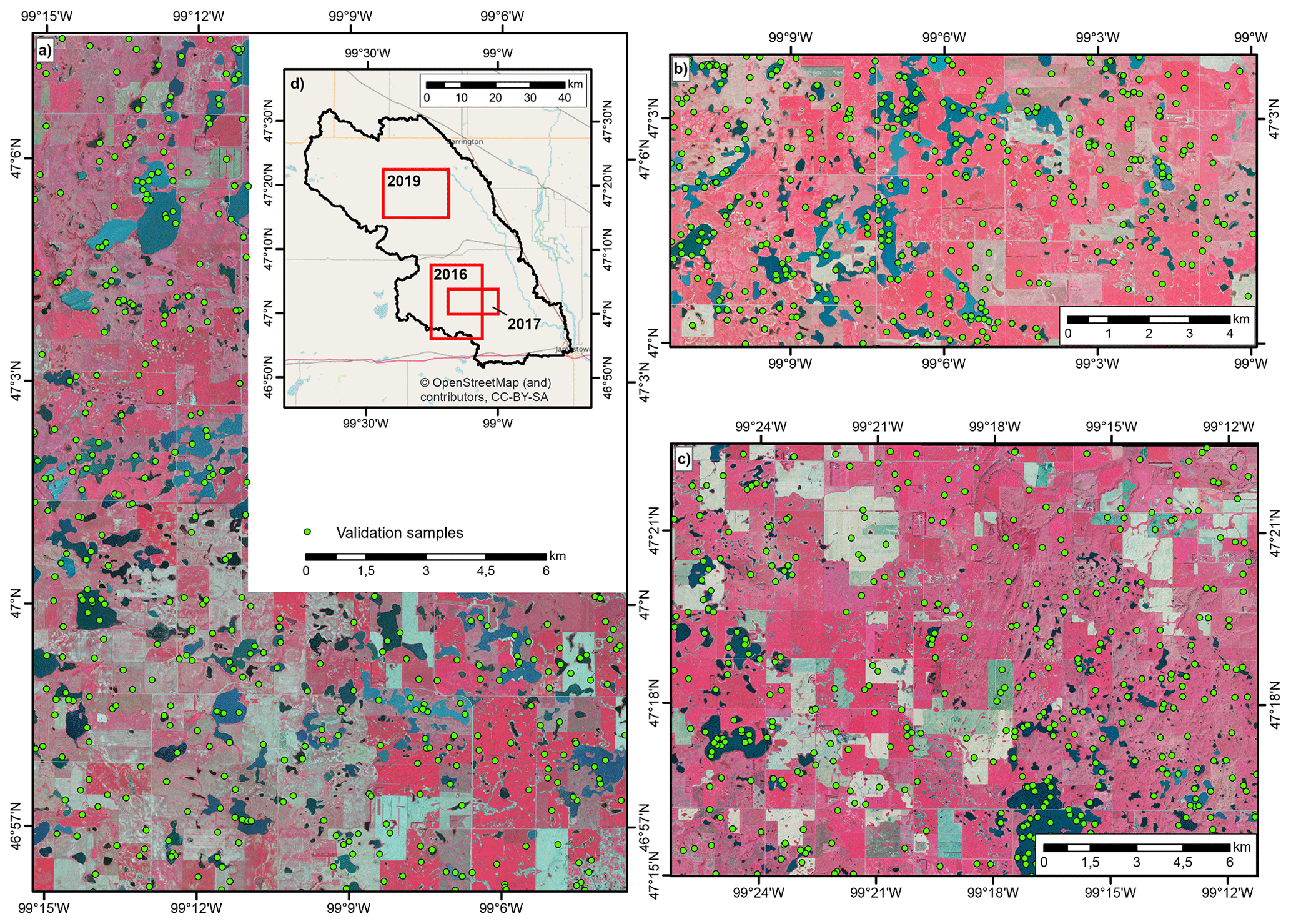
Figure A1 NAIP false-colour composites (R – near-infrared, G – red and B – green) acquired in (a) 2016, (b) 2017 and (c) 2019. Green dots show sample points used for the validation of waterbodies derived from Sentinel-1. (d) Location of the NAIP footprints inside the study area.

Appendix B: Probabilistic water maps

Figure B1 Maps of posterior probabilities, $p\left(W\right|{\mathit{\sigma }}_{\mathrm{p}}^{\mathrm{0}})$, for p=VH (in green) and p=VV (in blue) polarisations. Panel (a) corresponds to the binary maps shown in Fig. 6c, and panel (b) corresponds to the binary maps shown in Fig. 6d.