Citizen rain gauges improve hourly radar rainfall bias correction using a two-step Kalman filter

The low density of conventional rain gauge networks is often a limiting factor for radar rainfall bias correction. Citizen rain gauges offer a promising opportunity to collect rainfall data at a higher spatial density. In this paper, hourly radar rainfall bias adjustment was applied using two different rain gauge networks: tipping buckets, measured by Thai Meteorological Department (TMD), and daily citizen rain gauges. The radar rainfall bias correction factor was sequentially updated based on TMD and citizen rain gauge data using a two-step Kalman filter to incorporate the two gauge datasets of contrasting quality. Radar reflectivity data from the Sattahip radar station, gauge rainfall data from the TMD, and data from citizen rain gauges located in the Tubma Basin, Thailand, were used in the analysis. Daily data from the citizen rain gauge network were downscaled to an hourly resolution based on temporal distribution patterns obtained from radar rainfall time series and the TMD gauge network. Results show that an improvement in radar rainfall estimates was achieved by including the downscaled citizen observations compared with bias correction based on the conventional rain gauge network alone. These outcomes emphasize the value of citizen rainfall observations for radar bias correction, in particular in regions where conventional rain gauge networks are sparse.

1 Introduction

Hydrometeorological hazards, like flash floods and landslides, cause severe damage to economies, properties, and human lives worldwide. In this context, flood forecasting and warning systems are a valuable nonstructural measure to mitigate damage. However, such systems require the input of rainfall data at a high spatial and temporal resolution. In most regions of the world, automatic rain gauge networks are insufficient for this purpose. Weather radar, which can better capture the variation in rainfall fields at fine spatial and temporal resolutions, could be used as an alternative rainfall product to improve the accuracy of flash flood estimates and warnings. (Collinge and Kirby, 1987; Sun et al., 2000; Uijlenhoet, 2001; Bedient et al., 2003; Creutin and Borga, 2003; Mapiam et al., 2009a, 2014; Mapiam and Chautsuk, 2018; Corral et al., 2019). However, weather radar provides an indirect measurement of backscattered electromagnetic waves called radar reflectivity data (Z), and quantitative estimation of radar rainfall data (R) is acknowledged as a complex process. Various sources of error affect radar rainfall estimates, mainly errors in reflectivity measurements and reflectivity–rainfall conversion (Jordan et al., 2000). Correction of these two sources of error is a crucial procedure to increase the accuracy of radar rainfall estimates. “Ground truthing” by rain gauge data is required to calibrate the Z–R relationship (Z=AR^b). The calibrated parameter A in the Z–R relationship will include any errors in the radar system caused by the electrical calibration of the radar (Seed et al., 2002).

The calibrated Z–R equation is used to convert the measured instantaneous reflectivity data to rainfall intensity and, subsequently, to accumulate them into the required temporal resolution. However, the parameters A and b vary significantly, even within a single storm event, depending on the rainfall characteristics, which can exhibit a highly dynamic raindrop size distribution (DSD) (Ulbrich, 1983: Smith et al., 2009). Additionally, past studies have found that the Z–R parameters are sensitive to the temporal resolution of the rain gauge rainfall data that are used for the Z–R calibration (Hitchfeld and Bordan, 1954; Smith et al., 1975; Wilson and Brandes, 1979; Klazura, 1981; Steiner et al., 1995; Mapiam and Sriwongsitanon, 2008; Mapiam et al., 2009b). Consequently, an important source of error remains associated with the Z–R conversion process (Jordan et al., 2000; Berne and Krajewski, 2013). Many researchers have attempted to correct this kind of error by classifying the measured reflectivity data into different storm types and, thereafter, constructing the Z–R equation corresponding to the classified storm characteristics (Joss and Waldvogel, 1970; Rogers, 1971; Battan, 1973; Klazura, 1981; Austin, 1987; Rosenfeld et al., 1992, 1993; Tokay and Short, 1996; Amitai, 2000; Arai et al., 2005; Fang et al., 2018). To account for the effect of using rain gauge data with different temporal resolutions on the Z–R relationships, Mapiam et al. (2009b) developed a universal scaling transformation function for converting the reference parameters A (obtained from using daily gauge rainfall data in the calibration) to the parameter A for sub-daily resolutions. This improved the accuracy of the estimated sub-daily radar rainfall, especially in locations with limited short-duration rain gauge measurements.

After Z–R conversion, bias is expected to remain between the assessed radar rainfall and the true rainfall amount at the rain gauge locations if a fixed Z–R relationship is used to estimate radar rainfall over the entire radar domain (Chumchean et al., 2006; Wang et al., 2015). An effective bias correction technique is key for enhancing the quality of radar rainfall estimates (Steiner et al., 1999) and for removing the residual errors between radar rainfall obtained from the Z–R relationship and from the rain gauge data. Mean field bias (MFB) adjustment is the conventional method used to obtain a static bias factor which assumes that the Z–R relationship is homogeneous in space but varies in time (Smith et al., 2007; Vieux and Bedient, 2004; Wilson, 1970). In this method, a multiplicative correction factor is applied uniformly across the radar coverage. As the MFB approach does not consider the noise and uncertainty of the rain gauge observations nor the spatial variability in observation bias, this can lead to large errors in radar rainfall estimates, particularly in areas where the density of rain gauge networks is limited. The Kalman filter (KF) is an efficient algorithm that has been applied to correct the spatially uniform mean field bias, especially in real time by accounting for the temporal variation in the mean bias as well as uncertainties in the ground rainfall measurements (Anhert et al., 1986; Smith and Krajewski, 1991; Anagnostou et al., 1998; Seo et al., 1999; Dinku et al., 2002; Chumchean et al., 2006).

Previous studies have used the KF to predict and correct the mean field bias in order to mitigate the observation error variances affecting the mean field bias estimate. Chumchean et al. (2006) found that the density of the rain gauge network also plays an important role in the radar rainfall bias adjustment. They found that lowering the density of rain gauge observations in the KF process reduced accuracy of radar rainfall estimates. Additionally, the KF approach outperforms the use of MFB if the rain gauge density is less than one gauge per 90 km², and both KF and MFB produce identical performance when the rain gauge density is greater than one gauge per 70 km².

In basins where a dense rainfall network is not available, citizen science (CS) offers a promising opportunity to enhance the density of rainfall observations (Davids et al., 2019). With the popularization of smartphones and the availability of (relatively) simple and cheap equipment, abundant mobile applications and projects have been initiated in water resources management to measure hydrometeorological variables like rainfall, water level height, or water quality as well as to ground truth remotely sensed information on, for example, land use (Srivastra et al., 2018; Davids et al., 2019; See, 2019; Seibert et al., 2019). In the current study, we focus on rainfall measured by local citizens using a network of cheap rain gauges and a specially designed mobile application. As citizen rainfall observations are typically provided at a daily scale, a temporal downscaling technique is needed for sub-daily applications. A variety of temporal rainfall downscaling methods have been developed since the 1970s. The simplest approach is to distribute daily rainfall data to sub-daily resolutions by assuming uniform distributions. Stochastically generating subperiod data or spatially transferring finer-resolution rainfall from a nearby rain gauge station to the study area based on spatial correlations are alternative approaches (Koutsoyiannis, 2003; Debele et al., 2007). However, these methods are usually not designed for real-time data disaggregation over large areas. Instead, a common approach for such scenarios is to downscale daily rainfall based on a simple fraction technique by considering the distribution patterns of high-resolution gridded rainfall products from radar or satellite sensors (Paulat et al., 2008; Wüest et al., 2009; Vormoor and Skaugen, 2013; Sideris et al., 2014; Barton et al., 2020). This study aimed to modify the KF logic by integrating hourly rain gauge data with daily citizen rain gauge data that are downscaled to an hourly timescale using a simple fraction method. The radar rainfall bias correction factor was sequentially updated using a two-step Kalman filter accounting for the contrasting quality of the hourly rain gauge data and downscaled citizen rain gauge data. The question that we set out to answer is as follows: to what extent do the downscaled citizen rainfall observations improve the accuracy of hourly radar rainfall estimates? Several scenarios of hourly rainfall distribution patterns were applied for downscaling in order to investigate the most suitable technique for hourly radar rainfall assessment. Tubma Basin, located in Rayong Province, eastern Thailand, was used as a case study area to test the approach.

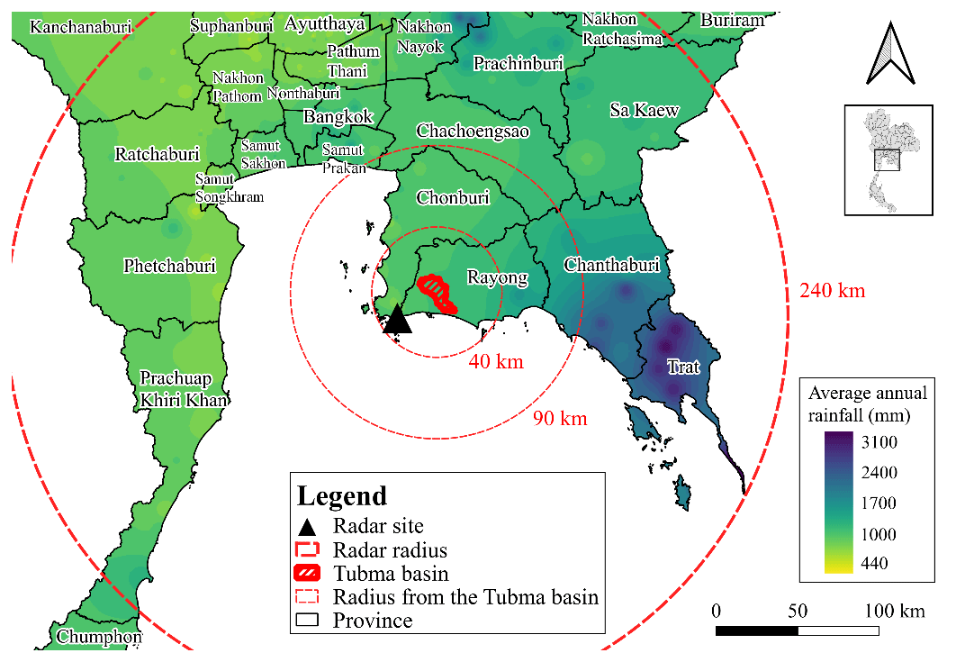
Figure 1 Climatological spatial rainfall distribution in and around the Tubma Basin calculated from 30-year average annual rainfall data from a rain gauge network of 311 daily gauges using the inverse distance squared (IDS) method.

2 Study area and data

2.1 Study area

The study area is the Tubma Basin (12.6789–12.8775^∘ N, 101.0881–101.2975^∘ E) located in Rayong Province, eastern Thailand (Fig. 1). It covers a catchment area of 197 km² with a basin elevation ranging from 4 to 416 m a.m.s.l. (above mean sea level). The main river, the Klong, is 42 km in length; originates in the Khao Chom Hae, Khao Ket, and Khao Krabok mountains; and flows downstream to the northwest before meeting the Gulf of Thailand in Pak Nam, Mueang Rayong District. The Tubma watershed is susceptible to flooding, in particular Rayong. In Fig. 1, we show the climatological variation across the study area and its surroundings, based on the 30-year (1987–2017) annual mean rainfall from a network of 311 daily rain gauges owned by the TMD and situated within 200 km of the Tubma Basin. Spatial rainfall patterns were generated using the inverse distance squared (IDS) method between the gauge locations. The map shows that while there is a small gradient in mean annual rainfall (1100–1700 mm mean annual rainfall) across the Rayong and Chonburi provinces (within 90 km of the study area), changes are more pronounced when the distance exceeds the 90 km boundary, especially to the east of the study area. This is because these areas are affected differently by the southwest monsoon. Consequently, the evaluation of the effectiveness of the bias correction techniques was carried out within a 90 km radius of the study area to ensure similar climatology.

2.2 Radar data

2.2.1 Reflectivity data collection

The Tubma Basin is located within the coverage of the Sattahip radar station. The Sattahip radar, which belongs to the Department of Royal Rainmaking and Agricultural Aviation (DRRAA), is an S-band Doppler radar that transmits radiation with a frequency of 2.9 GHz and a half-power beamwidth of 1.0^∘. The radar reflectivity product is provided on a Cartesian grid covering a 240×240 km extent with a 0.6×0.6 km spatial and 6 min temporal resolution. The Sattahip radar provides the reflectivity data derived from the 2.5 km constant altitude plan position indicator (CAPPI). The CAPPI reflectivity data originate from below the climatological freezing level, so the effects of measurement errors caused by the bright band were considered negligible. The effects of ground clutter were removed from the reflectivity data by finding the clutter locations and discarding the radar measurements in these areas. Additionally, the noise power caused by various sources, such as emission from space (cosmic noise), radiation from electrical sources near the radar antenna, and internally generated noise, were eliminated by setting reflectivity values below 15 dBZ to zero (Doviak and Zrnic, 1984). While Fulton et al. (1998) suggested that measured reflectivity values that are greater than 53 dBZ be limited to 53 dBZ in radar rainfall estimation to mitigate false interpretation caused by hail, the hail cap can be seen as an adaptable threshold representing the maximum expected instantaneous rain rate, which is unfortunately quite difficult to determine for a particular storm. Note that slightly higher hail threshold values have also been reported in tropical environments. After data quality control, we separated the data into three datasets: the first dataset from May to October 2013 and from May to September 2014 was used for the climatological Z–R calibration; the second dataset from October 2014 was used for the Z–R verification; and the third dataset from August to October 2019 was used in the bias correction processes.

2.2.2 The Z–R calibration and radar rainfall aggregation

The Z–R conversion error is a crucial source of error in radar rainfall estimates. The Z–R relationship was used to convert the measured reflectivity data (Z, mm⁶ m⁻³) into rainfall rates (R, mm h⁻¹). The Z–R calibration and verification are essential procedures to ascertain the A and b parameters in the relationship. Firstly, the instantaneous 6 min radar reflectivity was converted to rainfall intensity using the climatological relationship Z=200R^1.6 proposed by Marshall and Palmer (1948). Secondly, the estimated 6 min initial instantaneous radar rainfall data were aggregated to an hourly rainfall resolution using the accumulation algorithm proposed by Fabry et al. (1994). Thirdly, gauge rainfall was aggregated to an hourly resolution. Finally, the optimal value of the parameter A was established by minimizing the mean absolute error (MAE) between the gauge and the radar rainfall estimates, whereas the exponent b was 1.5 in our study. This is because radar rainfall estimates are relatively insensitive to b with typical values between 1.2 and 1.8 (Battan, 1973; Ulbrich, 1983). Thus, 1.5 was generally suitable to represent the exponent b in the Z–R relation (Doelling et al., 1998; Steiner and Smith, 2000; Hagen and Yuter; 2003; Germann et al., 2006; Chantraket et al., 2016). The MAE is illustrated in Eq. (1):

$$\begin{array}{}\text{(1)}& \mathrm{MAE}={\displaystyle \frac{\mathrm{1}}{T{N}_{\mathrm{G}}}}\sum _{t=\mathrm{1}}^T\sum _{i=\mathrm{1}}^{N_{\mathrm{G}}}\mathrm{|}{G}_{i,t}-R_{i,t}\mathrm{|},\end{array}$$

where G_i,t is the gauge rainfall (mm h⁻¹) at gauge i for hour t, R_i,t is the hourly radar rainfall accumulation (mm) at the pixel corresponding to the ith rain gauge for hour t, N_G is the total number of rain gauges, and T is the total period used in the calculation. Results found that the optimal climatological Z–R relationship for the Sattahip radar used in this study is Z=251R^1.5. This relation is appropriate for both the calibration and validation datasets with an MAE of 1.36 and 1.47 mm, respectively.

2.3 Rain gauge data

2.3.1 Rainfall data collection

Data from the network of 297 continuous tipping-bucket gauge stations located within the Sattahip radar radius were collected (Fig. 2). These rain gauges, which produce data with a temporal resolution of 15 min, are owned and operated by the Thai Meteorological Department (TMD). All of the continuous rain gauges used in this study have a resolution of 0.5 mm. The data quality screening was first carried out using the double-mass curve method. To avoid no-rainfall events and systematical underreporting by the tipping-bucket rain gauge, hourly data above the tipping-bucket resolution of 0.5 mm were selected in the next step. Rain gauges with more than 80 % of their recorded rainfall amounts below the 0.5 mm threshold at the daily scale were excluded from the analysis. It turns out that many of these faulty gauges recorded zero rainfall throughout most of the study period. Following the implementation of these criteria, rainfall data obtained from 134 rain gauges corresponding to the collected reflectivity datasets were used for the Z–R calibration and validation processes. For the bias adjustment computation, the selection of rain gauge networks with rainfall behavior similar to the study area is necessary. We selected 14 TMD rain gauges in the region surrounding the Tubma Basin (Rayong and Chonburi provinces), based a on spatial decorrelation analysis, for this the process.

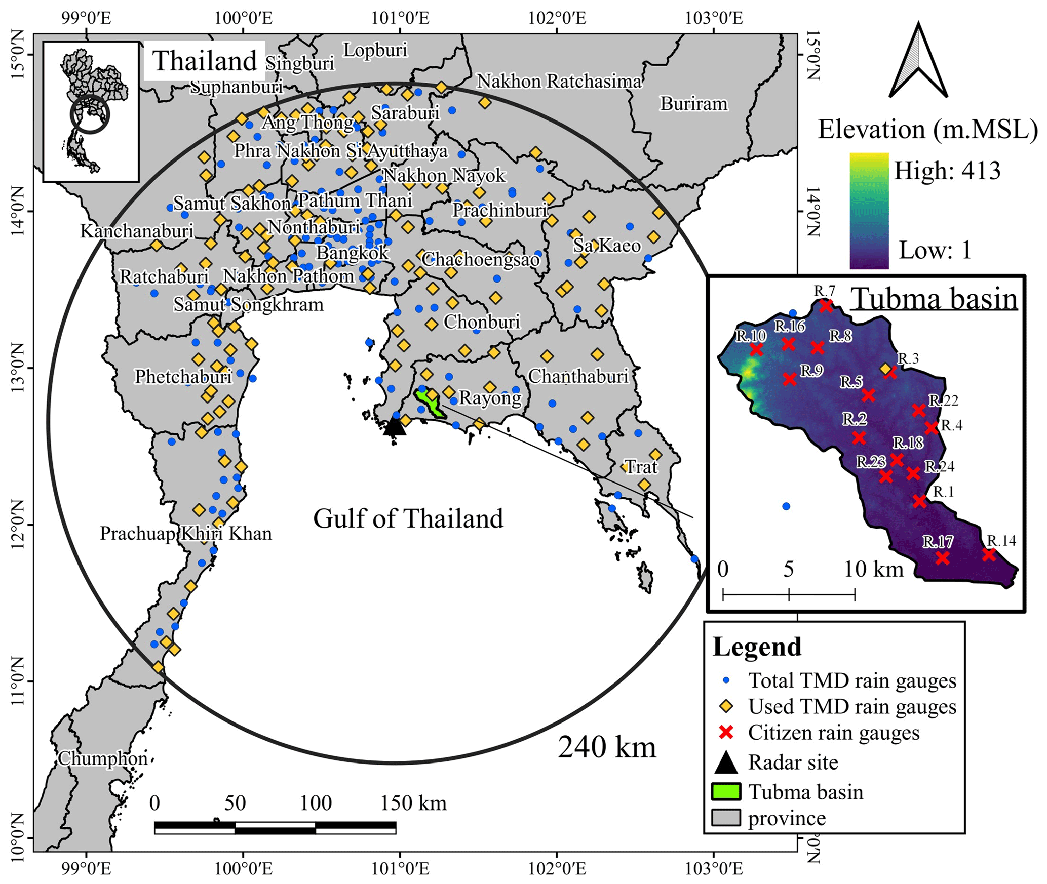
Figure 2 Location of the study domain, showing the Thai Meteorological Department (TMD) automatic rain gauges, the citizen rain gauges, the Sattahip radar, and the Tubma Basin.

2.3.2 Citizen rain observations

Out of the total TMD rain gauge network, only one rain gauge is located in the Tubma Basin. To increase the density of the rain gauge network in the basin, low-cost citizen rain gauges were implemented in this study to capture the spatial heterogeneity of rainfall in the region. A total of 16 citizen rain gauges were installed (Fig. 2) with local residents taking daily measurements. The additional 16 citizen rain gauges (with one station co-located with an existing TMD gauge) increased the density of rain gauges in the Tubma Basin to one gauge per ∼12 km². The citizen observations were made by installing a cone-shaped transparent plastic rain gauge in an open area around a school, monastery, bridge or other building. This type of rain gauge is in standard use in South Africa (Fig. A1) and has a diameter of approximately 12.7 cm (5 in.) and a maximum capacity of 100 mm of rainfall. A mobile application developed by Mobile Water Management (MWM) (Mobile Water Management, 2020), the Netherlands, was used to record rainfall data for each rain gauge on a daily basis. The application has a an easily accessible and user-friendly interface where participants simply fill in the observed rainfall amount, take a photo of the rain gauge, and upload the information to the application. The photo and the rainfall data, along with the measurement location and time, are automatically stored in the database. Photos are used for visual validation of the recorded rainfall depth in order to eliminate errors.

In this study, the participants recruited were government officers, teachers, and local residents living close to the stations; these participants were trained to take measurements at around 07:00 LT (local time) daily according to the TMD standards. The quality of the collected data was assured by double-checking the observations against the abovementioned high-resolution photos as well as by the strict requirements with respect to measurement times, which ensured consistency with the TMD daily rainfall recording standard. Validation of the cone-shaped citizen gauges was conducted based on a citizen gauge co-located with an automatic TMD gauge in the Tubma Basin, from August to October 2019. The citizen gauge installed at the same location as a TMD gauge (location R.3) showed good similarity with an RMSE and bias of 5.5 mm and 1.04, respectively (Fig. A2).

Quality control consisted of screening all citizen rain gauge data for errors and inconsistencies using double-mass curves. If citizen rain gauges reported >100 mm d⁻¹ rainfall (maximum capacity of the citizen rain gauge), these data were excluded from the analysis. If days with no-rainfall data were found from all citizen rain gauges, the bias correction of that day was discarded from the dataset. Considering these data selection criteria for rainfall data recorded from August to October 2019, more than 80 % of the whole period for the bias adjustment process was then used for further analysis.

3 Methods

The methodology for radar rainfall bias correction using tipping-bucket and citizen gauges consists of the following steps. Daily citizen rain gauge data were downscaled to an hourly timescale to be used as input for bias correction. The downscaling methods used in this paper are discussed in Sect. 3.1. Next, an hourly radar bias correction model was developed that combined rain gauge and downscaled citizen rain gauge data using a KF approach, as presented in Sect. 3.2.

3.1 Downscaling daily to hourly rainfall

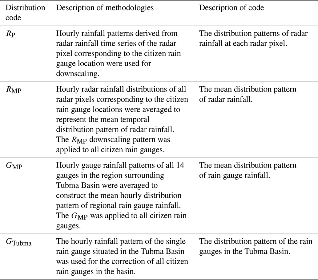
To downscale the daily citizen rain gauge data to an hourly timescale, information on the hourly storm distribution pattern is needed. Methodologies to obtain the temporal rainfall distribution patterns are outlined in Table 1.

Table 1 The four methods used in this study to downscale the daily citizen rainfall amounts to hourly rainfall data.

3.2 Hourly radar bias model

This section describes how radar bias is modeled (Sect. 3.2.1), how observations are assimilated in the model to correct the bias (Sect. 3.2.2), and how model parameters are estimated (Sect. 3.2.3). Our approach extends a previously used Kalman filter radar bias model by including two different types of rainfall observations (data from traditional and from citizen rain gauges) and using a likelihood-based method for parameter estimation.

3.2.1 Kalman filter with two observations: model assumptions

Mean field bias (MFB) adjustment is a common technique for bias correction in radar rainfall relative to ground stations. It can be computed as the ratio of the mean hourly radar rainfall estimate to the rain gauge measurement (Anagnostou and Krajewski, 1999; Yoo and Yoon, 2010; Hanchoowong et al., 2013; Shi et al., 2018). However, direct application of the MFB does not account for uncertainty in the bias associated with each radar-gauge measurement. Alternatively, a KF has previously been used to estimate the spatially uniform MFB in real time in several studies, including Anhert et al. (1986), Smith and Krajewski (1991), Anagnostou et al. (1998), Seo et al. (1999), Chumchean et al. (2006), Kim and Yoo (2014), and Shi et al. (2018). The KF has the benefit of accounting for uncertainties in the observations by weighting the contribution of measurements by their respective error variances (Kalman, 1960). This is also the approach adopted here, but we extend it to include two types of observations with different error characteristics, i.e., hourly rain gauge data from TMD (y_t) and hourly downscaled citizen rain gauge data (z_t).

Figure 3 Panel (a) presents a factor graph representation of the radar bias model: white circles depict random variables (bias at each time step), gray circles are rainfall bias observations (y_t for TMD rainfall, and z_t for citizen rain gauge rainfall), and black squares are relations between variables (conditional normal distributions in this case). Panel (b) depicts uncertainty propagation along the edges of the factor graph, from previous bias to current bias (Kalman prediction step in blue) and from the observations to current bias (two Kalman updates in red).

First, we define the logarithmic mean field radar rainfall bias β_t at hour t as follows (Smith and Krajewski, 1991; Anagostou et al., 1998):

$$\begin{array}{}\text{(2)}& {\mathit{\beta }}_t={\log }_{\mathrm{10}}\left({\displaystyle \frac{\sum _{i=\mathrm{1}}^{N_{\mathrm{G},t}}{G}_{i,t}}{\sum _{i=\mathrm{1}}^{N_{\mathrm{G},t}}{R}_{i,t}}}\right),\end{array}$$

where G_i,t and R_i,t are as defined in Eq. (1). Following previous studies (e.g., Smith and Krajewski, 1991; Chumchean et al., 2006), we model the logarithmic mean field radar rainfall bias as a first-order autoregressive (AR1) process with stationary variance. Radar bias at time t is expressed in terms of the bias at previous time (β_t−1) and the process noise (W_t):

$$\begin{array}{}\text{(3)}& {\displaystyle }& {\displaystyle }{\mathit{\beta }}_t=r_{\mathrm{1}}{\mathit{\beta }}_{t-\mathrm{1}}+W_t;W_t\sim N\left(\mathrm{0},{\mathit{\sigma }}_{\mathrm{W}}^{\mathrm{2}}\right),\text{(4)}& {\displaystyle }& {\displaystyle }{\mathit{\sigma }}_{\mathrm{W}}^{\mathrm{2}}=\left(\mathrm{1}-r_{\mathrm{1}}^{\mathrm{2}}\right){\mathit{\sigma }}_{\mathit{\beta }}^{\mathrm{2}}.\end{array}$$

Here, r₁ is the lag-one correlation coefficient of the time-varying bias β_t, W_t is a zero-mean random error with variance ${\mathit{\sigma }}_{\mathrm{W}}^{\mathrm{2}}$, and ${\mathit{\sigma }}_{\mathit{\beta }}^{\mathrm{2}}$ is stationary variance of the process. We consider two types of observations, y_t and z_t, of the unknown bias at time t, derived from the TMD and citizen rain gauges. Each observation is modeled as a random sample from a normal distribution conditioned on the underlying unknown bias with distinct measurement error variances ${\mathit{\sigma }}_{{\mathrm{M}}_{y,t}}^{\mathrm{2}}$ and ${\mathit{\sigma }}_{{\mathrm{M}}_{z,t}}^{\mathrm{2}}$:

$$\begin{array}{}\text{(5)}& {\displaystyle }& {\displaystyle }{y}_t={\mathit{\beta }}_t+M_{y,t};M_{y,t}\sim N\left(\mathrm{0},{\mathit{\sigma }}_{{\mathrm{M}}_{y,t}}^{\mathrm{2}}\right),\text{(6)}& {\displaystyle }& {\displaystyle }{z}_t={\mathit{\beta }}_t+M_{z,t};M_{z,t}\sim N\left(\mathrm{0},{\mathit{\sigma }}_{{\mathrm{M}}_{z,t}}^{\mathrm{2}}\right).\end{array}$$

Here, ${\mathit{\sigma }}_{{\mathrm{M}}_{y,t}}^{\mathrm{2}}$ and ${\mathit{\sigma }}_{{\mathrm{M}}_{z,t}}^{\mathrm{2}}$ are time-varying measurement error variances for the TMD and citizen rain gauges, respectively.

A factor graph representation of the radar bias and observation models is illustrated in Fig. 3a, with circles denoting random variables, and black squares denoting “factors” or relations between variables in the model.

The model contains two parameters, i.e., r₁ and ${\mathit{\sigma }}_{\mathit{\beta }}^{\mathrm{2}}$, that need to be specified, together with values for the measurement error variances, ${\mathit{\sigma }}_{{\mathrm{M}}_{y,t}}^{\mathrm{2}}$ and ${\mathit{\sigma }}_{{\mathrm{M}}_{z,t}}^{\mathrm{2}}$. Parameter estimation will be discussed in Sect. 3.2.3. Section 3.2.2 first describes how observations are assimilated assuming that the values of the parameters and the measurement error variances have been specified.

3.2.2 Kalman filter with two observations: data assimilation

Having defined the model, we describe how observations are assimilated into the model, resulting in adjustments of the estimated bias. While the regular Kalman filter has two steps (prediction and update), assimilating two observations at each time step involves three steps, i.e., a prediction followed by two updates. Figure 3b shows a visual depiction of the prediction and update steps as probabilistic information propagating along the edges of the factor graph. These three steps are as follows:

1. Time update step (prediction). The first step for each hour t computes the respective prior mean ${\widehat{\mathit{\beta }}}_t^{-}$ and variance $P_t^{-}$ of β_t as

   $$\begin{array}{}\text{(7)}& {\displaystyle }& {\displaystyle }{\widehat{\mathit{\beta }}}_t^{-}=r_{\mathrm{1}}{\widehat{\mathit{\beta }}}_{t-\mathrm{1}},\text{(8)}& {\displaystyle }& {\displaystyle }{P}_t^{-}=r_{\mathrm{1}}^{\mathrm{2}}{P}_{t-\mathrm{1}}+{\mathit{\sigma }}_{\mathrm{W}}^{\mathrm{2}}.\end{array}$$

   Here, P_t−1 is the posterior variance of β_t−1. For the first time step 0 (t=0), we assume β₀=0 (climatological logarithmic mean field bias) and $P_{\mathrm{0}}=(\mathrm{1}-r_{\mathrm{1}}^{\mathrm{2}}){\mathit{\sigma }}_{\mathit{\beta }}^{\mathrm{2}}$ (represents stationary process variance) (Smith and Krajewski, 1991; Chumchean et al., 2006).

2. The first measurement update step (first correction). The first update merges the bias prediction from step 1 with noisy observation y_t (with measurement error variance ${\mathit{\sigma }}_{{\mathrm{M}}_{y,t}}^{\mathrm{2}}$), resulting in posterior mean ${\widehat{\mathit{\beta }}}_{y,t}$ and variance P_y,t of β_t given by the Kalman update equations (Eqs. 9–11).

   $$\begin{array}{}\text{(9)}& {\displaystyle }& {\displaystyle }{K}_{y,t}=P_t^{-}{\left(P_t^{-}+{\mathit{\sigma }}_{{\mathrm{M}}_{y,t}}^{\mathrm{2}}\right)}^{-\mathrm{1}}\text{(10)}& {\displaystyle }& {\displaystyle }{\widehat{\mathit{\beta }}}_{y,t}={\widehat{\mathit{\beta }}}_t^{-}+K_{y,t}\left(y_t-{\widehat{\mathit{\beta }}}_t^{-}\right)\text{(11)}& {\displaystyle }& {\displaystyle }{P}_{y,t}=\left(\mathrm{1}-K_{y,t}\right)P_t^{-}\end{array}$$

   Here, K_y,t is the Kalman gain for assimilating observation y_t. If there is no observation available at time t, K_y,t is zero (mathematically, a missing observation is equivalent to an observation with infinite variance ${\mathit{\sigma }}_{{\mathrm{M}}_{y,t}}^{\mathrm{2}}$ in Eq. 9), and the previous equations reduce to not performing any update, i.e., the posterior mean and variance are equal to the prior mean and variance.

3. The second measurement update step (second correction). The second update is done using the posterior values from the first correction (${\widehat{\mathit{\beta }}}_{y,t}$ and P_y,t) as the prior values. The resulting respective Kalman gain and posterior mean and variance are given by

   $$\begin{array}{}\text{(12)}& {\displaystyle }& {\displaystyle }{K}_{z,t}=P_{y,t}{\left(P_{y,t}+{\mathit{\sigma }}_{{\mathrm{M}}_{z,t}}^{\mathrm{2}}\right)}^{-\mathrm{1}},\text{(13)}& {\displaystyle }& {\displaystyle }{\widehat{\mathit{\beta }}}_{z,t}={\widehat{\mathit{\beta }}}_{y,t}+K_{z,t}\left(z_t-{\widehat{\mathit{\beta }}}_{y,t}\right),\text{(14)}& {\displaystyle }& {\displaystyle }{P}_{z,t}=\left(\mathrm{1}-K_{z,t}\right)P_{y,t}.\end{array}$$

   If there is no observation available at time t, Kalman gain K_z,t is zero, and these equations result in no update being applied, i.e., the posterior mean and variance are the same as after the first update.

   As the logarithmic mean field radar rainfall bias β_t is assumed to be normally distributed, the mean field bias (B_t) is lognormally distributed with posterior mean at time t obtained from the posterior mean and variance of β_t (Smith and Krajewski, 1991):

   $$\begin{array}{}\text{(15)}& {\widehat{B}}_t={\mathrm{10}}^{\left({\widehat{\mathit{\beta }}}_{z,t}+\mathrm{0.5}{P}_{z,t}\right)}.\end{array}$$

   The overall procedure of sequentially assimilating and downscaling the data is referred to as CKF (Kalman filter combined with the citizen rain gauge data), and it is summarized by the flowchart in Fig. 4. Operationally, it is implemented as follows. First, as the citizen rain gauge data were received in the last hour of day i, before receiving the downscaled hourly citizen rain gauge data of day i, the ordinary KF and observed hourly data of TMD were used to predict and correct the hourly bias adjustment factor. Second, if the citizen rain gauge data were available at the end of the day i, they were downscaled to an hourly timescale, as explained in Sect. 3.1. Third, the TMD and downscaled citizen rain gauge data were used together to conduct two steps of measurement update in the CKF process for all hourly time steps of day i. Finally, bias adjustment factors were applied at every hourly time step to obtain the final product of hourly radar rainfall estimation of day i. The bias factor for the last hour of the day i was used afterward as the initial value for calculating the ordinary KF of day i+1.

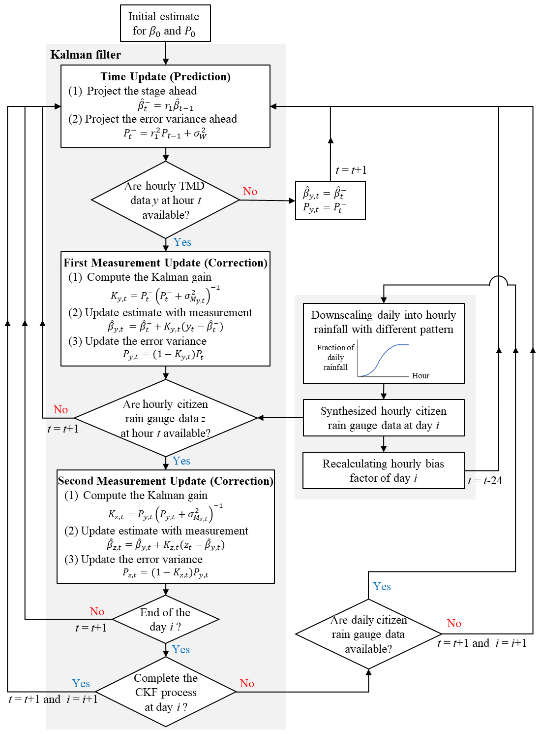
Figure 4 A diagram of the procedure of Kalman filter combined with the citizen rain gauge data (CKF).

3.2.3 Kalman filter with two observations: parameter estimation

The model requires specification of the two parameters, r₁ and $\mathit{\sigma }{}_{\mathit{\beta }}^{\mathrm{2}}$, and the measurement error variances, ${\mathit{\sigma }}_{{\mathrm{M}}_{y,t}}^{\mathrm{2}}$ and ${\mathit{\sigma }}_{{\mathrm{M}}_{z,t}}^{\mathrm{2}}$. We estimate the latter using formulas for the variance of the mean bias across individual TMD and citizen rain gauges:

$$\begin{array}{}\text{(16)}& {\displaystyle }& {\displaystyle }{\mathit{\sigma }}_{{\mathrm{M}}_{y,t}}^{\mathrm{2}}={\displaystyle \frac{{\mathit{\sigma }}_{y_t}^{\mathrm{2}}}{n_{y,t}}},\text{(17)}& {\displaystyle }& {\displaystyle }{\mathit{\sigma }}_{{\mathrm{M}}_{z,t}}^{\mathrm{2}}={\displaystyle \frac{{\mathit{\sigma }}_{z_t}^{\mathrm{2}}}{n_{z,t}}}.\end{array}$$

Here, ${\mathit{\sigma }}_{y_t}^{\mathrm{2}}$ and ${\mathit{\sigma }}_{z_t}^{\mathrm{2}}$ are variances that quantify spatial variability of radar bias at time t at TMD and citizen rain gauge locations, respectively, and n_y,t and n_z,t are the corresponding number of observations at hour tfrom the two networks.

Once measurement error variances are specified, values for parameters r₁ and ${\mathit{\sigma }}_{\mathit{\beta }}^{\mathrm{2}}$ are obtained by maximizing the marginal likelihood function (Bock and Aitkin, 1981; Harvey, 1990; Proietti and Luati, 2013; Pulido et al., 2018). As mentioned earlier, we have two sources of observed log mean field bias at hour t, from TMD (y_t) and citizen rain gauges (z_t). When only TMD data are available, the marginal likelihood is computed as follows:

$$\begin{array}{}\text{(18)}& \begin{array}{rl}p\left(\mathit{D}\right)& =\prod _{t=\mathrm{0}}^T\int p\left(y_t\mathrm{|}{\mathit{\beta }}_t\right)p\left({\mathit{\beta }}_t\mathrm{|}{y}_{t-\mathrm{1}},\mathrm{\dots },y_{\mathrm{0}}\right)d{\mathit{\beta }}_t\\ & =\prod _{t=\mathrm{0}}^{T}N\left(y_t;{\widehat{\mathit{\beta }}}_t^{-},{\mathit{\sigma }}_{y_t}^{\mathrm{2}}+P_t^{-}\right),\end{array}\end{array}$$

where D is the data vector that contains all observed values, β_t is the true hidden state of log mean field bias at hour t, and T is the number of hourly time steps. When both TMD and citizen rain gauge data are available, the marginal likelihood is obtained as follows:

$$\begin{array}{}\text{(19)}& \begin{array}{rl}p\left(\mathit{D}\right)& =\prod _{t=\mathrm{0}}^T\int p\left(y_t\mathrm{|}{\mathit{\beta }}_t\right)p\left(z_t\mathrm{|}{\mathit{\beta }}_t\right)p\left({\mathit{\beta }}_t\mathrm{|}{y}_{t-\mathrm{1}},z_{t-\mathrm{1}},\mathrm{\dots },y_{\mathrm{0}},z_{\mathrm{0}}\right)d{\mathit{\beta }}_t\\ & =\prod _{t=\mathrm{0}}^{T}N\left(y_t;z_t,{\mathit{\sigma }}_{{\mathrm{M}}_{y,t}}^{\mathrm{2}}+{\mathit{\sigma }}_{{\mathrm{M}}_{z,t}}^{\mathrm{2}}\right)N\left({\mathit{\tau }}^{-\mathrm{1}}\left({\displaystyle \frac{y_t}{{\mathit{\sigma }}_{{\mathrm{M}}_{y,t}}^{\mathrm{2}}}}+{\displaystyle \frac{z_t}{{\mathit{\sigma }}_{{\mathrm{M}}_{z,t}}^{\mathrm{2}}}}\right);\right.\\ & \left.{\widehat{\mathit{\beta }}}_t^{-},{\mathit{\tau }}^{-\mathrm{1}}+P_t^{-}\right),\end{array}\end{array}$$

where $\mathit{\tau }=\frac{\mathrm{1}}{{\mathit{\sigma }}_{{\mathrm{M}}_{y,t}}^{\mathrm{2}}}+\frac{\mathrm{1}}{{\mathit{\sigma }}_{{\mathrm{M}}_{z,t}}^{\mathrm{2}}}$ and prior mean ${\widehat{\mathit{\beta }}}_t^{-}$ and variance $P_t^{-}$ are from the prediction step in Sect. 3.2.2.

To obtain optimal values of the two parameters r₁ and ${\mathit{\sigma }}_{\mathit{\beta }}^{\mathrm{2}}$ that maximize the (logarithm of the) marginal likelihood, the Nelder–Mead simplex was used, which is an algorithm for searching a local optimum of a function (Lagarias et al., 1998; Luersen and Le Riche, 2004; Gao and Han, 2012).

Table 2 Simulation cases for evaluating the effectiveness of bias correction techniques.

^* CKF-H includes four scenarios for four different hourly downscaling patterns for the citizen rain gauges, according to Table 1.

3.3 Verification of the proposed bias correction approaches

To investigate which bias adjustment technique (MFB, KF, and CKF) gives the most suitable radar rainfall estimates for the Tubma Basin, the adjusted radar rainfall estimates were validated against measured rainfall data. There was only one automatic TMD rain gauge available in the basin, which was insufficient for validation purposes. Consequently, to test the performance of the hourly rainfall bias correction, data from 13 TMD stations located within a 90 km radius of the center of the Tubma Basin were used in addition to the one TMD station in the basin. Furthermore, daily timescale validation was conducted, using the daily rainfall data from 16 citizen rain gauges located in the Tubma Basin. A leave-one-out cross-validation (LOOCV) algorithm was implemented to avoid bias in selecting the validation rain gauges. For each round of cross-validation, one rain gauge was left out for validation, and the remaining rain gauges were used as the calibration rain gauges to calculate the bias adjustment factor using the three different techniques. This was repeated for all combinations, and the error of radar rainfall estimates after correction with the estimated bias factor at each radar pixel corresponding to the held-out gauge was then computed for all trials. In this study, the root-mean-square error (RMSE) and mean bias error (MBE) were applied as statistical measures to evaluate the effectiveness of the different bias correction methods at each validation rain gauge. The number of possible combinations is equal to the total number of validated gauges (N_G). Data for the period from August to October 2019 were used in the evaluation. Four scenarios combining the three bias adjustment techniques were evaluated, as summarized in Table 2. These four scenarios are as follows:

1. KF-TMD-H – 1 TMD rain gauge from the 14 total gauges was left out for validation, and the remaining 13 gauges were separated to calculate the bias adjustment factors using the MFB and KF. This process was iterated 10 times until all 14 TMD rain gauges were left out for cross-validation. Aggregated hourly rainfall values between the adjusted radar and the gauge rainfall data were compared to obtain the RMSE and MBE.

2. F-TMD-D – to identify whether the MFB or KF is more accurate for daily rainfall simulation in the Tubma Basin if there are only 14 TMD rain gauges available, 14 TMD and 16 citizen rain gauges were used for the analysis. All TMD gauges were used for assessing the MFB and KF, and estimated bias factors were applied at the daily timescale. An assessment of the RMSE and MBE of daily rainfall at all 16 citizen rain stations was used for validation.

3. CKF-D – to evaluate the added value of using citizen rain gauges in the basin for bias correction, 15 citizen rain gauges (leave one citizen rain gauge out for validation) were used in addition to the TMD gauges following the CKF procedure explained in Sect. 3.2.2. Estimation of the daily RMSE and MBE was carried out at the held-out citizen rain gauge.

4. CKF-H^* – to test whether the CKF with the most suitable storm pattern could benefit radar rainfall estimates in the area further away from the Tubma Basin, 14 TMD gauges were used to generate four cases of hourly rainfall distribution patterns, as described in Table 1, for downscaling the selected 16 daily citizen rain gauge data to an hourly timescale. The synthesized hourly citizen rain gauge data were later used as a second observation for the second correction of the CKF. A total of 13 TMD gauges (leave one TMD out) were used to produce estimates with the MFB and KF, and all 16 citizen rain gauges were merged for CKF computation.

All bias adjustment techniques evaluated the effectiveness at the held-out gauge for all possible combinations of the LOOCV procedure.

4 Results and discussion

4.1 Simulation of the bias adjustment factor

4.1.1 Parameter estimation for the KF and CKF

Five scenarios were investigated for radar bias correction using the KF, based on TMD and citizen rain gauge observations, including four scenarios comparing different hourly downscaling approaches for the citizen rain gauge data (Table 1). Parameter estimates of the KF are shown in Table 3. These results indicate that the parameter r₁, the lag-one correlation coefficient of the logarithmic mean field bias, ranges from 0.15 to 0.53, depending on the hourly downscaling approach, whereas ${\mathit{\sigma }}_{\mathit{\beta }}^{\mathrm{2}}$, representing the stationary variance of the logarithmic mean field bias, remains relatively invariant (ranging from 0.24 to 0.28) over the same period of simulation.

Table 3 The parameters of the KF estimated from different datasets of observation gauge rainfall. KF-TMD only uses TMD hourly rain gauge observations; CKF uses TMD and citizen rain gauge observations, where R_P, R_MP, G_MP, and G_Tubma represent different strategies for hourly downscaling of the citizen rain gauge observations (Table 1).

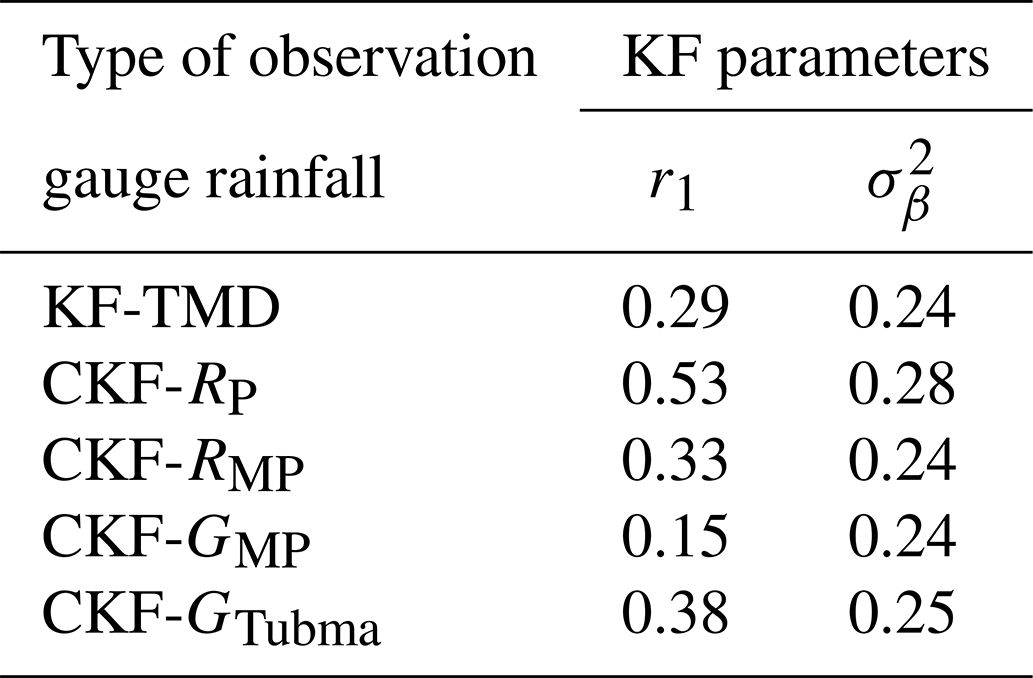
Figure 5 Comparison of (a) daily observed mean field bias based on TMD rain gauges in the region and the citizen rain gauges in the Tubma Basin, (b) hourly observed mean field bias based on TMD rain gauge observations and downscaled citizen rain gauge observations, (c) hourly observation error variances, and (d) hourly estimated mean field bias obtained based on the MFB and the five different KF approaches. Bias calculations cover 16 citizen gauges in the Tubma Basin and 14 TMD gauges within a 90 km radius of the Tubma Basin. Hourly scale calculations for the citizen gauges (CKF) are based on four different sub-daily interpolation scenarios (R_P, R_MP, G_MP, and G_Tubma; Table 3).

4.1.2 Bias adjustment factor comparison

To test the performance of the bias adjustment techniques among KF-TMD, CKF-R_P, CKF-R_MP, CKF-G_MP, and CKF-G_Tubma, all approaches were used to assess the mean field bias for each hour using the data period from August to October 2019. The results were compared to the MFB calculated using the 14 TMD rain gauges (MFB-TMD) in the Tubma Basin and within a 90 km radius of the basin. The results summarized in Fig. 5 show the following:

• The daily observed bias is somewhat higher and shows larger variability for the citizen gauges compared with the TMD gauges. The hourly observed bias values based on downscaled citizen gauge data are in the same range as hourly bias values based on TMD gauges, with somewhat higher median values and spread (25–75 percentile range) for the R_P and G_Tubma downscaling scenarios.

• The hourly observation error variance is smallest for the CKF-R_P downscaling approach and somewhat larger for the other CKF approaches compared with the observation error variance for the TMD gauges.

• Estimated hourly bias values based on KF-TMD show a slightly higher mean and a smaller variability range compared with observations. The bias produced by the KF-TMD is close to the MFB-TMD if the observation error variance is small. In the case that no measured data are available for the bias update, the computed bias factor (B_t) progressively converges to 1.3, to meet the climatological logarithmic mean field bias.

• Estimated bias values based on the CKF approaches are able to reproduce bias variability as observed by TMD gauges, with median values deviating by 0.2–0.4 and the value range being slightly larger for CKF-R_P and smaller for CKF-R_MP.

• CKF gives different bias values according to the storm distribution pattern (see Appendix B) and the availability of the daily citizen rain gauge data used in combination with the KF. In the case that no citizen rain gauge data are available for updating, the bias generated by the CKF for every combination is close to the ordinary KF with small differences depending on their respective r₁ and ${\mathit{\sigma }}_{\mathit{\beta }}^{\mathrm{2}}$ parameters.

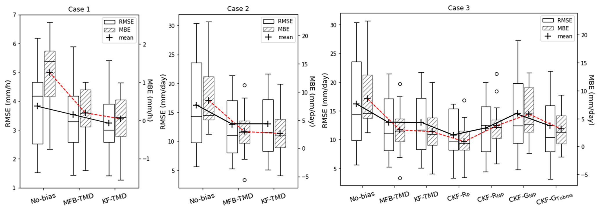
Figure 6 Variation in RMSE and MBE across the cross-validation scenarios for the various evaluation cases: (a) case 1, hourly bias updating based on the MFB and KF using TMD gauges; (b) case 2, daily bias updating based on the MFB and KF using only TMD gauges; and (c) case 3, daily bias updating using the MFB, KF (TMD gauges), and CKF (TMD and citizen gauges). Validation covers 16 gauges in the Tubma Basin for the daily scale and 14 gauges within a 90 km radius of the Tubma Basin for the hourly scale.

4.2 Effectiveness evaluation of bias correction approaches

4.2.1 Hourly rainfall validation for the larger region (90 km radius) surrounding Tubma Basin using the MFB and KF approaches (case 1)

Figure 6a shows cross-validation results based on the RMSE and MBE between TMD rain gauges and adjusted radar rainfall using the MFB and KF for hourly bias adjustment. Bias adjustment reduces the RMSE and, especially, the MBE, with KF-TMD performing somewhat better than the MFB-TMD (especially in terms of the RMSE). This confirms the ability of the KF approach that considers the error variance of observed hourly data as the weight for correcting the predicted mean bias instead of using only the calculated mean field bias (Smith and Krajewski, 1991; Chumchean et al., 2006).

4.2.2 Daily rainfall validation in the Tubma Basin using the MFB and KF approaches with citizen gauges for validation (case 2)

Results associated with validating the bias correction performance within the Tubma Basin are presented in Fig. 6b. This shows bias correction performance within the Tubma Basin for the MFB and KF-based daily bias adjustment. The two approaches show similar performance at the daily scale and improve the RMSE by 20 %–30 % and the MBE by 50 %–60 % (for median and upper 75percentile, respectively). The added value of a KF-based approach is limited for this case, as 14 TMD rain gauges in the region were used to compute observation variance which cannot represent the mean field bias behavior in the Tubma Basin.

4.2.3 Daily rainfall validation in the Tubma Basin using the CKF approach (case 3)

Figure 6c shows cross-validation results at the daily scale for the Tubma Basin, comparing bias correction approaches using TMD only and TMD combined with citizen gauges. Following the CKF steps, citizen rain gauge data are downscaled to an hourly timescale using four different approaches, resulting in variation in hourly observed bias and error variances, as shown in Fig. 5b and c, respectively. Cross-validation results after accumulation to the daily scale show that CKF-R_P outperforms the other approaches (CKF-R_MP, CKF-G_Tubma, MFB-TMD, KF-TMD, and CKF-G_MP) in terms of both the RMSE and MBE. The performance of the CKF techniques for radar rainfall simulation in the Tubma Basin relates to the reliability of the downscaled hourly observations. This is reflected in the variation in the estimated observation error variances for CKF-R_P, as shown in Fig. 5b and c. The better performance of CKF-R_P is explained by the smallest range in observation error variance, which is indicative of better consistency observation bias. In comparison with the “No-bias” scenario, CKF-R_P can improve the RMSE by 32 %–25 % and can improve the MBE by 90 %–80 % for the median and upper 75 percentile, respectively. In contrast, CKF-G_MP exhibits the worst performance compared with the other CKF approaches, with a 13 %–16 % improvement in the RMSE and an 57 %–56 % improvement in the MBE for the median and upper 75 percentile, respectively. This apparent decrease in the efficiency of the CKF can be confirmed by the highest median value of the estimated observation error variances of CKF-G_MP (see Fig. 5c), which is 33 % higher than that of CKF-R_P.

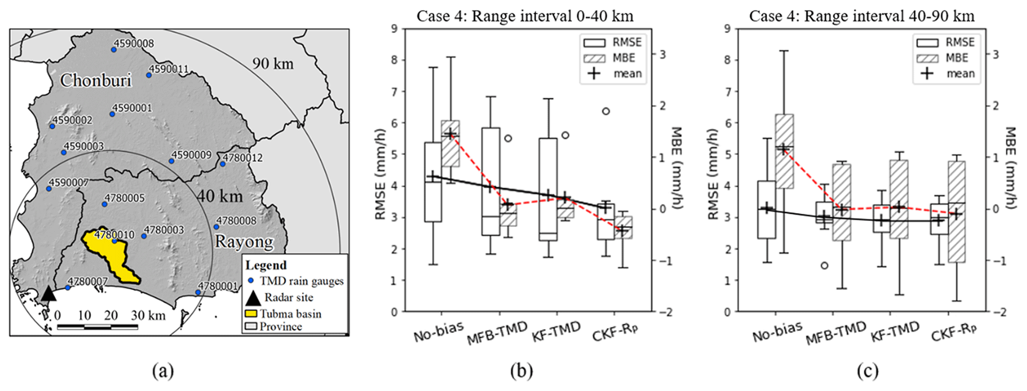
Figure 7 Comparison of the RMSE and MBE for different range intervals from the center of the Tubma Basin. Panel (a) shows the rain gauge locations at each range interval, panel (b) shows comparisons for the 0–40 km range, and panel (c) shows comparisons for the 40–90 km range. For CKF, only results for the CKF-R_P approach are shown, based on its better performance at the daily timescale (shown in Fig. 6c).

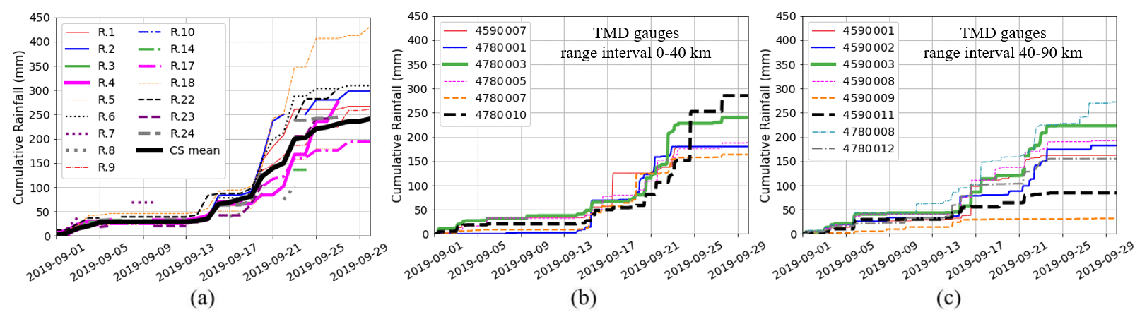
Figure 8 Comparison of mass curves of hourly rainfall among various rain gauge locations for (a) the citizen rain gauges located in the Tubma Basin, (b) TMD rain gauges within a 0–40 km radius of the Tubma Basin, and (c) TMD rain gauges within a 40–90 km radius of the Tubma Basin.

4.2.4 Hourly rainfall validation using the MFB, KF, and CKF approaches (case 4)

Results for this section are presented in Figs. 7 and 8. The performance for radar rainfall estimates using CKF-R_P with different distances from the Tubma Basin is reported in Appendix C. Cross-validation results at an hourly timescale show a strong improvement achieved by bias adjustment using citizen gauges, in particular close to the Tubma Basin where the citizen gauges are located. Figure 7b and c show validation results based on TMD gauges for gauges close to (0–40 km radius) and further away from (40–90 km radius) the center of Tubma Basin (see Fig. 7a); both ranges cover a similar number of TMD gauges. Figure 7b and c show that CKF-R_P bias adjustment significantly improves radar rainfall estimates at an hourly timescale, compared with bias adjustment approaches based on TMD gauges only in the 0–40 km range closest to the Tubma Basin. While there is a modest improvement in the mean RMSE (see the black line connecting the mean values of the box plots from the MFB-TMD to CKF-R_P), the upper 75 percentile RMSE is reduced from about 6 to 3.5 mm h⁻¹. The mean MBE is changed from 0.1 to −0.15 mm h⁻¹ (see the red dotted line connecting the mean values from the MFB-TMD to CKF-R_P). For the 40–90 km range, CKF-R_P performs similarly to the MFB-TMD and KF-TMD.

Figure 8 illustrates that hourly rainfall distribution patterns of TMD rain gauges in the 0–40 km range, which are mainly influenced by the southwest monsoon, appear to be more similar to the mean citizen rain gauge data than the range beyond 40 km. Consequently, the application of CKF-R_P based on combining the citizen rain gauge network with the TMD rain gauge network (with similarity of rainfall characteristic) is key for improving radar rainfall estimates.

The results in Fig. 7 also show that the MBE values in the 0–40 km range are explicitly lower than those in the 40–90 km range. Apparently, at shorter range, positive and negative errors represented in the MBE cancel out more frequently than they do for the gauges at larger distance. In other words, gauges more or less randomly over- or underestimate rainfall values: we can see similar rainfall distribution patterns among all gauges, although there is high variation in the rainfall amount during the storm period in Fig. 8b. Conversely, in the 40–90 km range, bias correction at gauge locations consistently leads to over- or underestimation of rainfall. This can be explained by gauges at larger distances from the center of the basin being affected by different rainfall generation patterns, associated with their location closer to the coast or mountains (see Fig. 7a). The influence of the southwest monsoon strongly affects all gauges located in the coastal region on the windward side of a mountain, whereas rain gauge locations on the leeward side experience less rainfall. Figure 8c shows that TMD gauges located on the leeward side (e.g., 4590009 and 4590011) obviously appear as a steady gradient of the mass curve, reflecting light rainfall accumulation, whereas gauges on the windward side (e.g., 4590002 and 4590003) show mass curves with a sharper gradient. Further details on the sensitivity bias adjustment techniques' accuracy with respect to rainfall characteristics are provided in Appendix D.

5 Conclusion

In this study, we introduced a modified KF approach in radar bias correction in the Tubma Basin, eastern Thailand. The two-step KF integrates daily data from a dense citizen rain gauge network with hourly data from a much sparser network of conventional higher-quality tipping-bucket rain gauges. Daily citizen rain gauge observations were downscaled to an hourly timescale using four different approaches. The question that we aimed to answer was as follows: to what extent do the downscaled citizen rainfall observations improve the accuracy of hourly radar rainfall estimates? Results showed that citizen rain gauges significantly improve the performance of radar rainfall bias adjustment, up to a range of about 40 km from the center of the Tubma Basin (197 km²) where the citizen rain gauge network is located. While a modest improvement in the mean RMSE was obtained, the upper 75 percentile RMSE was reduced from 6 to 3.5 mm h⁻¹. The MBE was changed from 0.1 to −0.15 mm h⁻¹ across the validation period (August–October 2019). In the Tubma Basin, beyond the 40 km range, no significant improvement from the inclusion of the citizen gauges was found. The rainfall distribution pattern is key for downscaling the daily measured citizen rain gauge observations to an hourly temporal resolution. In the study region, we found that downscaling based on the rainfall patterns derived from hourly radar rainfall at overlying radar pixels corresponding to the citizen gauge location was the most suitable technique, resulting in the smallest variation in observation error variances of the mean field bias. In the case of a sparse rain gauge network, the mean field bias and the Kalman filter approach both show improvement, and the degree of improvement was similar between the two approaches. In other words, in a sparse gauge network, the added value of error information represented in the Kalman filter is limited. Note that citizen rain gauge data are available only at the end of the day; consequently, the modified two-step Kalman filter, as used in this study, has limitations with respect to real-time applications. However, the method proposed here has clear potential when creating high-quality historical radar-rainfall time series for climatological studies and in post-event analysis. Moreover, near-real-time assessment could be achievable if the citizen rain gauge data were collected at a sub-daily timescale.

Appendix A: Citizen rain observation and validation

An example of installing a cone-shaped transparent plastic citizen rain gauge (in standard use in South Africa) at location R.22 (Map Tong school, Rayong Province) is illustrated in Fig. A1. Validation of the cone-shaped citizen gauges was done at location R.3 by comparing the measured daily citizen gauge data with a co-located automatic TMD gauge, as presented the result in Fig. A2. The root-mean-square error (RMSE) and bias were applied as statistical measures for the validation as shown in Eqs. (A1) and (A2), respectively:

$$\begin{array}{}\text{(A1)}& {\displaystyle }& {\displaystyle }\mathrm{RMSE}=\sqrt{{\displaystyle \frac{\mathrm{1}}{T}}\sum _{t=\mathrm{1}}^T{\left(G_{\mathrm{TMD},t}-G_{\mathrm{CR},t}\right)}^{\mathrm{2}}},\text{(A2)}& {\displaystyle }& {\displaystyle }\mathrm{bias}={\displaystyle \frac{\sum _{t=\mathrm{1}}^T{G}_{\mathrm{TMD},t}}{\sum _{t=\mathrm{1}}^T{G}_{\mathrm{CR},t}}}.\end{array}$$

Here, G_CR,t is daily citizen gauge rainfall at location R.3 for day t, G_TMD,t is daily TMD gauge rainfall at the same location of R.3 for day t, and T is the total period used in the calculation.

Figure A1 An example of installing a cone-shaped transparent plastic citizen rain gauge at location R.22 (Map Tong school).

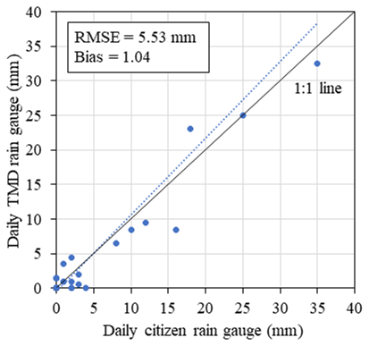
Figure A2 Daily rainfall depth comparison between the co-located TMD and citizen rain gauge at location R.3 from August to October 2019.

Appendix B: Hourly rainfall distribution patterns

Four hourly rainfall distribution patterns were obtained, as outlined in Table 1. Figure B1 illustrates the cumulative fraction of daily rainfall at the hourly scale during the simulation period from August to October 2019. It can be seen that most rainfall was concentrated in the afternoon hours, with very little rainfall falling at night. R_P and R_MP showed relatively more rainfall concentrated in the afternoon, while R_P and G_MP showed larger variability in the downscaled hourly data with substantial outliers in the box plots, which were associated with the variability in the locations underlying the rainfall distributions (multiple radar pixels within the Tubma Basin for R_P versus multiple TMD gauges surrounding the Tubma Basin for G_MP). G_MP showed the flattest distribution with the longest rainy period of around 11 h compared with the others which had a period of heavy rainfall of around 4–5h d⁻¹. This is explained by the larger spatial variability in the gauges covered by G_MP.

Figure B1 Variation in the fraction of 24 h rainfall for each rainfall distribution scenario.

Appendix C: The performance of radar rainfall estimates using CKF-R_P with different distances from the Tubma Basin

We chose the 40 km separation boundary to achieve an equal number of gauges in the “near” and “far” groups. Following the referee's comment, we investigated the RMSE between gauge rainfall and radar rainfall without bias adjustment (RMSE_No-bias) and with the CKF-R_P (RMSE_CKF-RP) for individual stations (located at distances of 5–80 km from the Tubma Basin). We computed the percentage improvement in radar rainfall estimates using CKF-R_P compared with No-bias at each rain gauge, indicating that the relative errors change with distance from the Tubma Basin (Fig. C1). Figure C1 shows that the improvement percentage of using CKF-R_P tends to decrease with increasing distance from the Tubma Basin, where the citizen gauges are located. The percentage reduction gradually decreases beyond a distance of about 40 km.

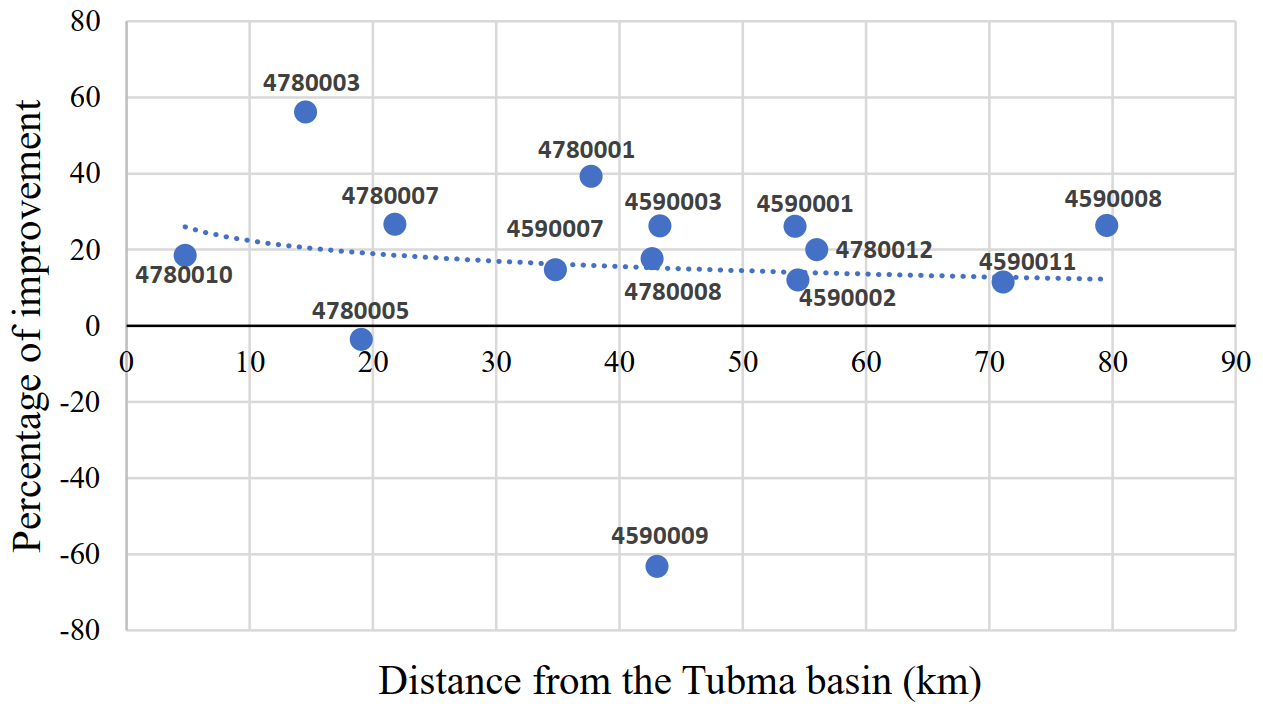
Figure C1 Alteration of the percentage improvement in radar rainfall estimates using CKF-R_P compared with No-bias at each rain gauge with different distances from the Tubma Basin.

Note that gauge 4780010, situated nearest to the basin, is expected to provide the best improvement; however, the Sattahip radar temporarily stopped measuring for 3 h (from 16:00 to 19:00 LT on 24 September 2019) due to the presence of a heavy storm's center that was only observed at this gauge. This leads to significant degradation of the radar rainfall performance. Furthermore, the lower percentage improvement for station 4780005 is associated with a localized heavy rainfall event that was only recorded at this location and negatively affected its performance as a representative station for bias correction.

Appendix D: Investigation of rainfall characteristics affecting the accuracy of bias adjustment techniques

Figure 7b shows that the upper 75 percentile RMSE of the shorter range is remarkably high while using only TMD gauges for the bias adjustment. These errors occurred for 3 h at three different gauge locations when heavy rainfall data were only measured at the validated gauge location while there was relatively uniform light rainfall at all available surrounding TMD gauges used for the bias adjustment calculation. Consequently, the calculated bias factors from the available gauges could not represent the heavy rainfall at the tested location, leading to the significant RMSE. An analysis of hourly rainfall hyetographs obtained from the TMD rain gauge network compared with the validated rain gauge occurring on 3 different days is illustrated in Fig. D1. It shows a considerable RMSE for 3 h on 3 d – 15 September 2019, 12:00 LT; 21 September 2019, 15:00 LT; and 22 September 2019, 14:00 LT – associated with the validated gauges, 4780001, 4780005, and 4780003, respectively. However, these RMSE values decrease considerably if the CKF-R_P was only implemented in the shorter range.

Figure D1 Hourly rainfall hyetographs obtained from the TMD rain gauge network compared with the validated rain gauge for 3 different days: (a) a storm event on 15 September 2019 based on using 4780001 as the validated gauge, (b) a storm event on 21 September 2019 based on using 4780005 as the validated gauge, and (c) a storm event on 22 September 2019 based on using 4780003 as the validated gauge.

Indeed, Fig. 8a and b show that one of the citizen gauges (R.18) collected a cumulative monthly rainfall amount that was higher than the range of the other citizen and TMD rain gauges. This is associated with a storm event that occurred in September 2019 (the storm center was over R.18, while the surroundings received appreciably less rainfall). Figure D2 shows the radar reflectivity field at 13.00 LT on 22 September 2019, during the peak of the storm, confirming the heavy rainfall affecting gauge location R.18. This shows that the citizen gauge network is able to capture local storm features thanks to the high density of the network. The multiple reporting gaps visible in Fig. 8a are caused by time errors in the observations submitted by local residents which were removed from the analysis (as explained in Sect. 2.3.2).

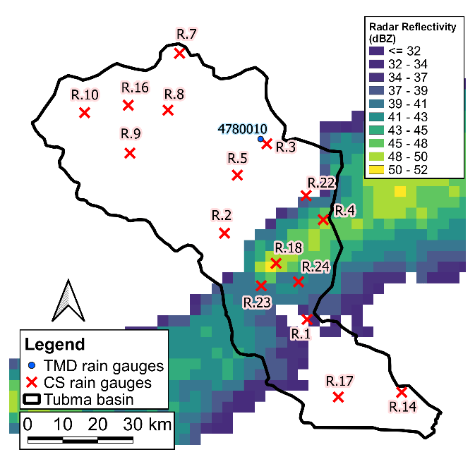
Figure D2 Overlap between the citizen rain gauge network and the spatial radar reflectivity data on 22 September 2019 at 13:00 LT.