the Creative Commons Attribution 4.0 License.
the Creative Commons Attribution 4.0 License.
 | 06 Jan 2022
Improved representation of agricultural land use and crop management for large-scale hydrological impact simulation in Africa using SWAT+
Celray James Chawanda
Jonas Jägermeyr
Ann van Griensven
To date, most regional and global hydrological models either ignore the representation of cropland or consider crop cultivation in a simplistic way or in abstract terms without any management practices. Yet, the water balance of cultivated areas is strongly influenced by applied management practices (e.g. planting, irrigation, fertilization, and harvesting). The SWAT+ (Soil and Water Assessment Tool) model represents agricultural land by default in a generic way, where the start of the cropping season is driven by accumulated heat units. However, this approach does not work for tropical and subtropical regions such as sub-Saharan Africa, where crop growth dynamics are mainly controlled by rainfall rather than temperature. In this study, we present an approach on how to incorporate crop phenology using decision tables and global datasets of rainfed and irrigated croplands with the associated cropping calendar and fertilizer applications in a regional SWAT+ model for northeastern Africa.
We evaluate the influence of the crop phenology representation on simulations of leaf area index (LAI) and evapotranspiration (ET) using LAI remote sensing data from Copernicus Global Land Service (CGLS) and WaPOR (Water Productivity through Open access of Remotely sensed derived data) ET data, respectively. Results show that a representation of crop phenology using global datasets leads to improved temporal patterns of LAI and ET simulations, especially for regions with a single cropping cycle. However, for regions with multiple cropping seasons, global phenology datasets need to be complemented with local data or remote sensing data to capture additional cropping seasons. In addition, the improvement of the cropping season also helps to improve soil erosion estimates, as the timing of crop cover controls erosion rates in the model. With more realistic growing seasons, soil erosion is largely reduced for most agricultural hydrologic response units (HRUs), which can be considered as a move towards substantial improvements over previous estimates. We conclude that regional and global hydrological models can benefit from improved representations of crop phenology and the associated management practices. Future work regarding the incorporation of multiple cropping seasons in global phenology data is needed to better represent cropping cycles in areas where they occur using regional to global hydrological models.
- Article
(4350 KB) - Full-text XML
- BibTeX
- EndNote


Even though cropland cultivation covers over 40 % of the planet's ice-free land surface, most regional and global hydrological model applications overlook the necessity of addressing crop phenological development and/or distinguishing between different crops (Chen and Xie, 2012; Srivastava et al., 2020). In some regional applications (e.g. Schuol and Abbaspour, 2006; Schuol et al., 2008; Chawanda et al., 2020), the model applications consider one uniform generic crop as a simplification for agricultural land use representation despite the existing wide variety of crops in agricultural land use (Sood and Smakhtin, 2015). Using a uniform generic crop for agricultural land use modelling fails to account for any variability in vegetation attributes, such as leaf area index (LAI), corresponding to several crops in real-world scenarios (Viña et al., 2011). Detailed agricultural land use representation in hydrological models is important as heterogeneity in agricultural land use can have a significant effect on hydrological fluxes such as evapotranspiration (ET) and soil moisture (Srivastava et al., 2020). Through ET and interception (Siad et al., 2019), the water balance of agricultural land use areas is strongly influenced by the applied management practices (e.g. planting, irrigation, fertilization, and harvesting) and their precise timing (Twine et al., 2004; Raymond et al., 2008). In the context of global change studies, a realistic representation of agricultural systems is a major concern as changes in climatic factors affect crop growth and the productivity of agricultural systems (Makowski et al., 2014). Therefore, hydrological models that simulate cropland ecosystems should have a reasonable representation of crop phenology and the associated management practices of these ecosystems (Lokupitiya et al., 2009).
The SWAT+ model (Bieger et al., 2017; Arnold et al., 2018), which is a restructured version of SWAT (Soil and Water Assessment Tool; Arnold et al., 1998) utilizes the principles of the Environmental Policy Integrated Climate (EPIC) crop growth model (Williams and Singh, 1995) to simulate agricultural land by default in a generic way, where the phenological development of crops from planting is driven by accumulated heat units (Arnold et al., 1998). However, the primary controlling factor for the start of the growing season in tropical and subtropical regions such as sub-Saharan Africa is rainfall (Lotsch et al., 2003; Alemayehu et al., 2017). Waha et al. (2013) describes the crop growing season in sub-Saharan Africa as the period in which temperature and moisture are suitable for growth determined by the start and end of the main rainy season. Zhang et al. (2005) showed that the onset of seasonal vegetation green-up across Africa can be directly linked to rainfall seasonality. Several studies (e.g. Msigwa et al., 2019; Nkwasa et al., 2020) have further pointed out how the existing multiple cropping seasons in tropical and subtropical climates within an agricultural year coincide with the rainfall and irrigation patterns. Therefore, the use of heat units to trigger the start of the cropping seasons could lead to inconsistencies in crop phenology simulations for tropical and subtropical regions.
Croplands include various types with associated differences in crop physiology and management practices (Lokupitiya et al., 2009; Yin and Struik, 2009). The phenological change during the vegetation cycle of crop types actively controls the ET process through internal physiology by increasing the number of leaf stomata with canopy growth (Gong et al., 2014). In the SWAT+ model, plant transpiration is simulated as a linear function of leaf area index (LAI) and potential evapotranspiration (PET; Neitsch et al., 2005). Thus, inconsistences in crop simulations could lead to inaccurately estimating canopy properties such as LAI and canopy height, resulting in uncertain estimates of ET (Alemayehu et al., 2016). Accurate estimations of ET in a hydrological model are important because ET is the central flux that defines land–atmosphere interactions (Mueller et al., 2011; Fisher et al., 2017).
Additionally, changes in cropland use and crop management have received little attention in hydrological impact assessments, yet these may have significant impacts on model outputs (O'Neal et al., 2005). For example, Sietz et al. (2021) demonstrated the sensitivity of key hydrological processes (runoff, groundwater seepage, and ET) to crop rotations in a central European region by combining a crop generator with an ecohydrological model. By coupling a hydrological model (Variable Infiltration Capacity – VIC) with a crop growth model, soil moisture and ET were more accurately simulated by implementing crop rotations (Zhang et al., 2021). According to Abaci and Papanicolaou (2009), cropland use and cropland management practices can significantly affect the impact of rainfall on soil erosion. The crop canopy often intercepts rainfall and hinders water droplets to reduce the splash erosion through loss of speed (Hilker et al., 2014). In addition, cropland practices cause great variations in the erodibility of cropland since soil erosion depends on what crop is grown and the crop cover density (Sundborg and White, 1982). The crop cover is crucial in the estimation of the C (crop management) factor in erosion models such as the Modified Universal Soil Loss Equation (MUSLE) used by SWAT+ (Lin et al., 2014). Other crop management practices, such as the amount of fertilizer, alters the soil's ability to produce biomass and, thus, alters soil resistance to erosion (Souza et al., 2017). The timing and duration of soil cover on cropland are affected by the planting and maturity dates of the crop.
Previous studies have applied the SWAT model at a regional scale within and including sub-Saharan Africa (Schuol and Abbaspour, 2006; Schuol et al., 2008). However, these studies utilized the default generic way of representing agricultural land use without any management practices. Yet, Arnold et al. (2012) emphasized the need for a realistic representation of local and regional crop processes to reliably simulate the water balance, erosion, and nutrient yields in a SWAT model. Chawanda et al. (2020) describe one of the few regional applications of the latest SWAT+ version in a tropical region. The study highlighted that the inclusion of irrigation and reservoirs in the model set-up, using decision tables (Arnold et al., 2018), led to an improvement in the simulations of discharge and ET. Hence, there is need to have a proper representation of land use and agricultural processes in Africa, as very few studies report on crop phenology and land use representation in SWAT (Griensven et al., 2012).
Regional cropping phenology datasets and management practices have been developed using remote sensing approaches (Li et al., 2014; Estel et al., 2016; Xiong et al., 2017) and non-remote sensing approaches, including observational census data (Potter et al., 2010; Portmann et al., 2010; Lu and Tian, 2017; Iizumi et al., 2019; Hurtt et al., 2020; Jägermeyr et al., 2021), to integrate into regional agricultural and hydrologic modelling frameworks. However, remote sensing approaches have been criticized as not being able to detect crop types and cropping sequences without local knowledge or ground truth data (Bégué et al., 2018). Nevertheless, these spatially explicit global cropping phenology datasets have not been utilized in regional hydrological models to improve the land use and crop representation.
The novelty of this study is in improving land use and crop process representation for large-scale hydrological modelling using SWAT+ by the following: (1) proposing an approach that reasonably incorporates crop phenology using decision tables and global datasets of rainfed and irrigated croplands with the associated management practices in a regional SWAT+ model for northeastern Africa; (2) evaluating model improvements of crop representation by using the remote sensing LAI from Copernicus Global Land Service (CGLS) and ET derived from WaPOR (Water Productivity through Open access of Remotely sensed derived data; FAO, 2018); and (3) evaluating how the consideration of crop phenology and the associated management practices affects long-term water-driven soil erosion estimates. We do not intend to fully model soil erosion but show to how improvements in crop representation can impact soil erosion estimates.
2.1 Study area
Our study focused on the northeastern part of Africa (Fig. 1) that covers 4 489 000 km2 for a period of 7 years (2009–2015). This area wholly (or partially) covers countries of the Nile Basin, including Uganda, Kenya, Tanzania, Rwanda, Burundi, Sudan, South Sudan, Ethiopia, and Egypt.
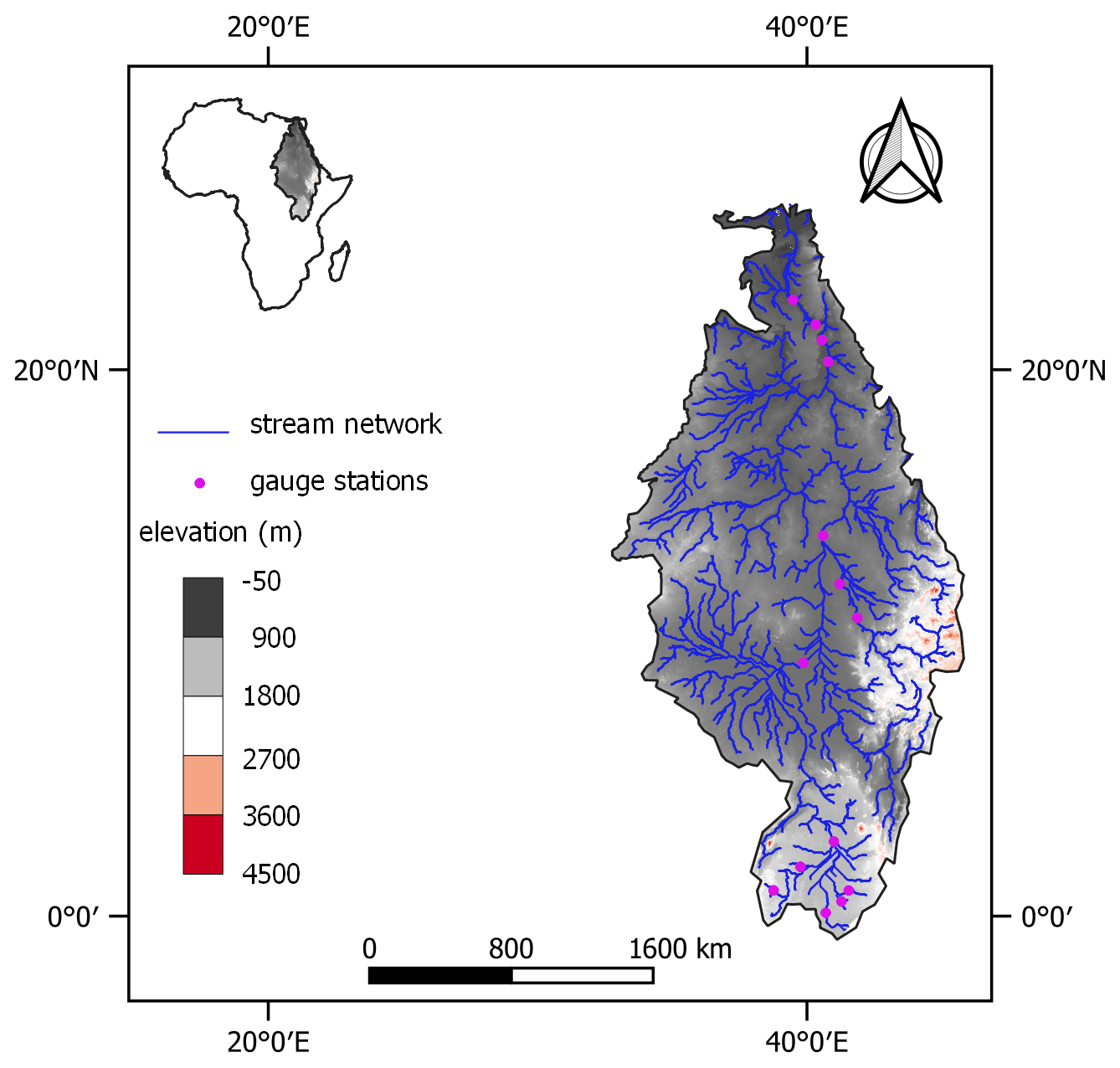
Figure 1The study area in northeastern Africa (Nile Basin).
The area includes the main Nile River basin with subbasins, such as the Blue Nile, White Nile, Atbara, Baro–Akobo–Sobat, Bahr El Jebel, and Bahr El Ghazal. The major basins are the Blue Nile basin and the White Nile basin. The Blue Nile basin, which originates from Lake Tana in Ethiopia is considered as the major tributary to the main Nile River due to its high contribution towards the total Nile River discharge. The White Nile starts from the great lakes region through Lake Victoria, Uganda, and South Sudan (Eldardiry and Hossain, 2019). A strong latitudinal wetness gradient characterizes the climate of the region. The area north of 18∘ N remains dry mostly of the year, while there is a gradual increase in monsoon rainfall amounts in the south (Camberlin, 2009). The distribution of the mean annual rainfall is spatially contrasted in the region, with about 28 % of the region receiving less than 100 mm annually. Rainfall in excess of 1000 mm yr−1 is restricted mainly to the equatorial region and the Ethiopian highlands, with negligible rainfall (below 50 mm yr−1) from northern Sudan and across all of Egypt (Onyutha and Willems, 2015). The agricultural sector is responsible for nearly 75 % of the water withdraw within the basins (Swain, 2011). Agriculture is practised in all elevation categories but predominantly in the low-lying areas (less than 500 m) and medium areas (890–1450 m). Shrubland is dominant in elevation areas ranging between −47 to 1450 m and in steep slopes, while forest is dominant in areas with an elevation range of 500 to 2150 m. In low-lying areas, mainly in the desert area of the Nile, bare land is dominant (Nile Basin Initiative, 2016).
2.2 Modelling approach using SWAT+
SWAT+ is a revised version of SWAT that offers greater flexibility in connecting spatial units in the representation of management operations (Bieger et al., 2017; Arnold et al., 2018). This is a semi-distributed river-basin-scale model that relies on the physical characteristics of a catchment. It divides a basin into subbasins connected by a stream network, which are further divided into hydrologic response units (HRUs). HRUs represent areas within the subbasin that comprise of the same land use, soil, slope, and management practices (Neitsch et al., 2005). SWAT+ also introduces landscape units (LSUs) to allow separation of lowland (wetland) processes from upland process (Bieger et al., 2017). SWAT+ applies the hydrological water balance concept, with Eq. (1) as the basic driver of all hydrological processes.
where WBf and WBi are the final and initial soil water content, respectively (millimetres per day; hereafter mm d−1), Pj is the amount of rainfall (mm d−1), Rj is the amount of surface runoff (mm d−1), Ej is the ET amount (mm d−1), Dj is the percolation amount (mm d−1), RFj is the return flow amount (mm d−1), Δt is the change in time (days), and j is the index. The model estimates erosion and sediment yield for each HRU, using the Modified Universal Soil Loss Equation (MUSLE; Williams and Berndt, 1977; Eq. 2). The MUSLE uses runoff energy rather than rainfall to estimate sediment yields, making it suitable at daily timescales.
where Sed is the sediment yield (tonnes per day; hereafter t d−1), Qsurf is the surface runoff volume (mm d−1), qpeak is the peak runoff rate (cubic metres per second; hereafter m3 s−1), Areahru is the area of the HRU (hectares), KUSLE is the Universal Soil Loss Equation (USLE) soil erodibility factor, CUSLE is the USLE crop management factor, PUSLE is the USLE support practice factor, LSUSLE is the USLE topographic factor, and CFRG is the coarse fragment factor.
2.2.1 Decision tables in SWAT+
Land use and management operations in SWAT+ can be scheduled by using either decision tables or management schedules or both. However, decision tables enable the user to model intricate sets of rules and their subsequent actions by allowing them to add conditions for scheduling management (Arnold et al., 2018). Metzner and Barnes (2014) describe decision tables as a way of organizing and documenting complex events in a logical way so that it is easy to interpret. Nkwasa et al. (2020) compared the use of decision tables to management schedules and concluded that decision tables provided higher flexibility in representing agricultural practices. The use of decision tables in the SWAT+ model is broadly described in (Arnold et al., 2018). Scheduling in this study was done using decision tables as discussed in the subsequent sections.
2.2.2 Crop growth cycle with heat unit scheduling
SWAT+ uses the simplified version of the EPIC growth model to simulate plant growth (Neitsch et al., 2005). As in the EPIC model, phenological plant development is based on the daily accumulated heat units or by calendar dates, while plant growth can be inhibited by temperature, water, nitrogen, and phosphorus nutrients (Neitsch et al., 2005; Arnold et al., 2012). The heat unit theory assumes that plants have requirements that can be quantified and linked to maturity. The total number of heat units required by the plant to start growing or to reach maturity is calculated as in Eq. (3).
where PHU is the total heat units required to plant maturity, Tav is the mean daily temperature (degrees Celsius), Tbase is the plant's minimum temperature for growth (degrees Celsius), d=1 is the day of planting, and n is the number of days required for a plant to reach maturity. Planting is scheduled by a second heat index, where heat units are summed over the entire year using Tbase=0 ∘C. This heat index is solely a function of climate calculated by SWAT+ using the provided long-term weather data (Neitsch et al., 2005). While scheduling by heat units is convenient for temperate regions that are mainly driven by temperature, users need to consider that cropping seasons in tropical and subtropical regions are primarily driven by water availability (Alemayehu et al., 2017). Hence, the use of heat units easily leads to incorrect cropping seasons for these regions.
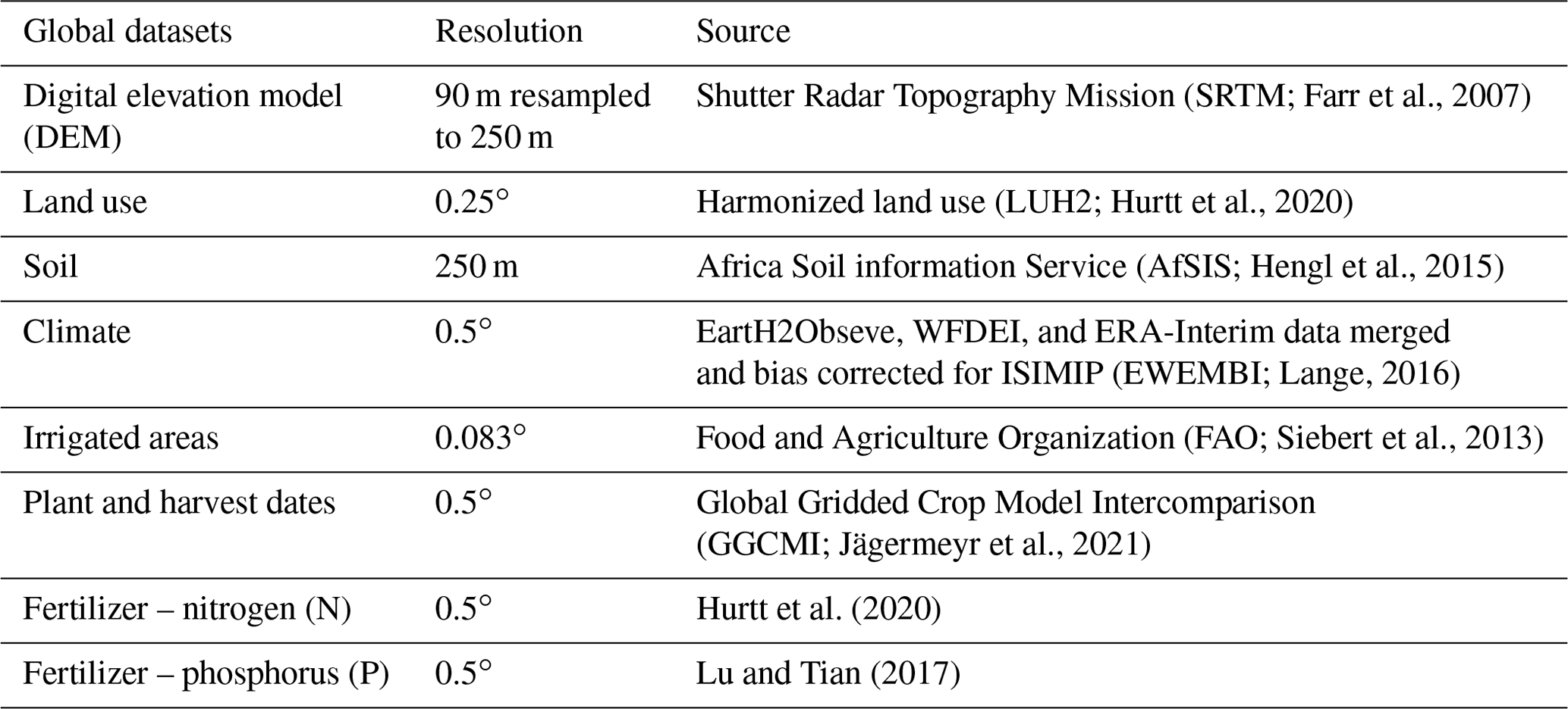
2.3 Global datasets used for SWAT+ modelling
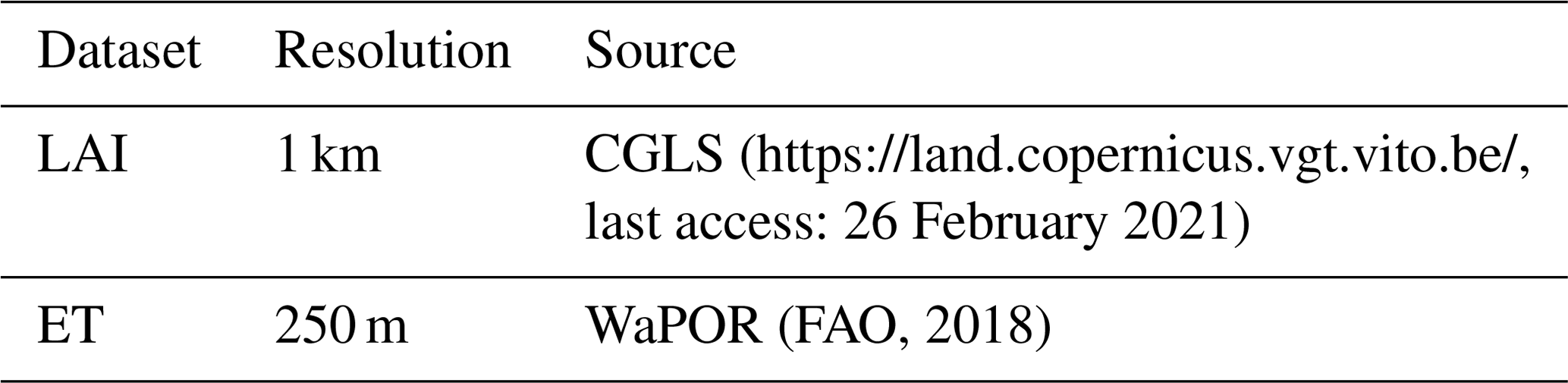
Modelling was done using the freely available global datasets in Table 1. Of specific interest in this study is the GGCMI dataset (Jägermeyr et al., 2021), which provides a cropping calendar that is an observation-based product, combining first-hand data sources from various agricultural ministries. In the GGCMI crop calendar, the planting dates and cultivar selection are based on real-world observational planting and harvest data. Planting, thus, happens at the prescribed day per crop in each 0.5∘ grid cell, and on average, cultivars are selected to match the observational harvest day. The development of this dataset is explicitly discussed in Jägermeyr et al. (2021). The climate data (EWEMBI; Lange, 2016) includes records of rainfall, maximum and minimum temperature, wind speed, solar radiation, and relative humidity available at a spatial resolution of 0.5∘. Irrigation data (Food and Agriculture Organization – FAO, 2018; Siebert et al., 2013) were provided as the area fraction equipped for irrigation and the area fraction that is actually irrigated per year. Nitrogen fertilizer and phosphorus fertilizer were provided as a global time series of gridded synthetic fertilizer use rate in agricultural lands at a spatial resolution of 0.5∘.
2.4 Spatiotemporal analysis of rainfall
Rainfall distribution and amount determines the suitability of crops and related agronomic management at different locations (Muthoni et al., 2019). Thus, long-term mean for the annual rainfall of the study period (2009–2015) was generated and plotted to visualize regional spatiotemporal patterns. The annual spatiotemporal variation in rainfall (interannual variability) was analysed by calculating the coefficient of variation (CV) in Eq. (4). Additionally, long-term mean monthly rainfall for the region was analysed to identify the seasonality of the monthly rainfall as the success or failure of the crop is more dependent on seasonal rainfall distribution (Ngetich et al., 2014).
where mean and SD are the mean rainfall and standard deviation for a selected temporal scale. According to Asfaw et al. (2018), CV is used to classify the degree of variability in rainfall events as low (CV < 20 %), moderate (20 % < CV < 30 %), and high (CV > 30 %).
2.5 Default model set-up
The SWAT+ model (revision 60.5) was set up with the QGIS (Quantum Geographic Information System) interface, using the data in Table 1 and run for a period of 7 years (2009–2015). The harmonized land use product (LUH2; Hurtt et al., 2020) used in this study is formatted as NetCDF; hence, the SWAT+ code had to be adapted to include subroutines to read the NetCDF data, using an approach proposed by Chawanda et al. (2020). The land use map is a composite of land use layers, with each layer representing a fraction of a given land use. The fraction layers representing cropland include; C3 annual crops (C3ann), C3 perennial crops (C3per), C4 annual crops (C4ann), C4 perennial crops (C4per), and C3 nitrogen-fixing crops (C3nfx). In the default model set-up, the cropland use in the land use map was represented with a uniform generic crop as per the default in the SWAT+ database (Arnold et al., 2013) for all the heterogenous cropland areas and heat units used to trigger the cropping seasons.
The study area was discretized into 768 landscape units and 12 526 unsplit HRUs. The USDA Soil Conservation Service (SCS) curve number method was used to estimate surface runoff, the variable storage method was selected for flow routing, and the Penman–Monteith method (Monteith, 1965) was used to calculate the potential evapotranspiration.
2.6 Proposed scheduling in the revised SWAT+ model – crop scheduling with global phenology datasets
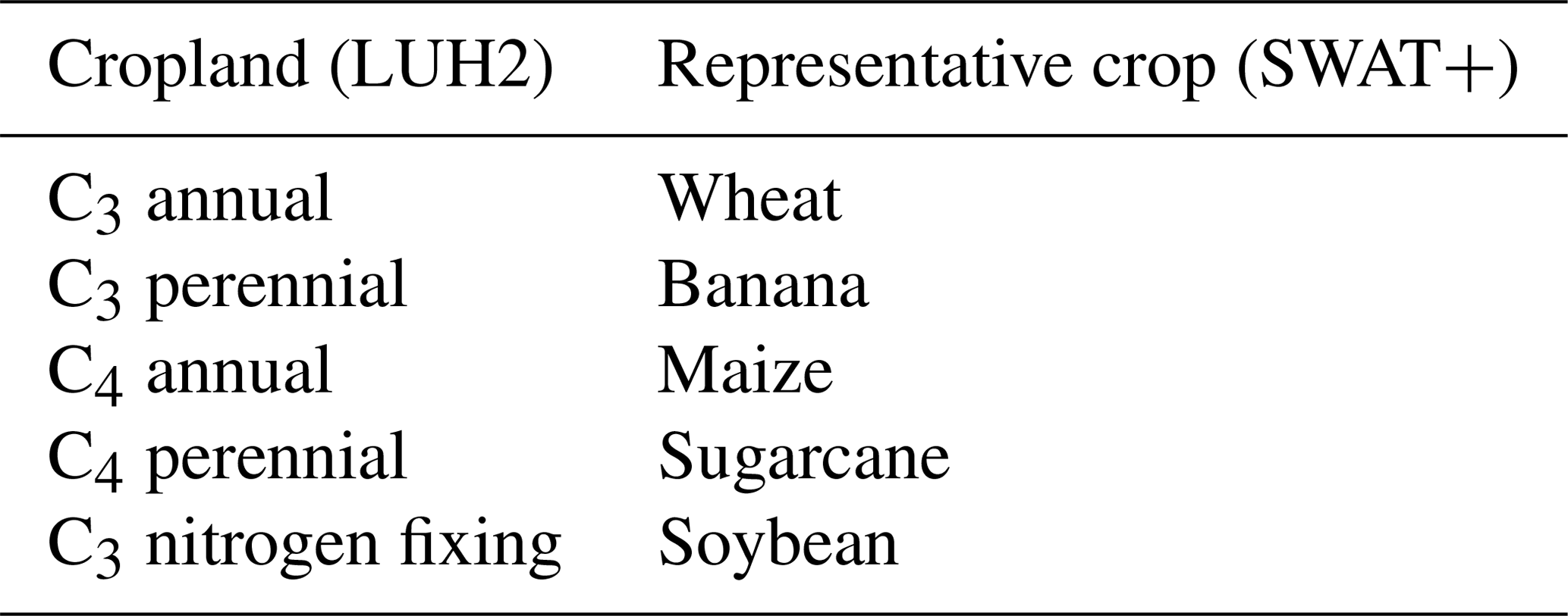
In the proposed scheduling, the fraction layers (C3ann, C4per, C4ann, C4per, and C3nfx) representing cropland in the land use map (LUH2) were extracted, and a comparison was made on a pixel-by-pixel basis. Whichever crop layer fraction occupied a larger percentage for the rainfed and irrigated agricultural areas within a pixel was selected to represent cropland for irrigated and rainfed areas in that pixel. For example (in Fig. 2), if the C4ann and C3nfx crop occupied a larger fraction within a pixel compared to other cropland use fraction layers for irrigated and rainfed cropland, respectively, then they were selected to represent cropland use in that pixel. A crop map was developed from this pixel-by-pixel analysis, and a representative crop was selected for each cropland use fraction based on the literature (Leff et al., 2004), as shown in Table 2.
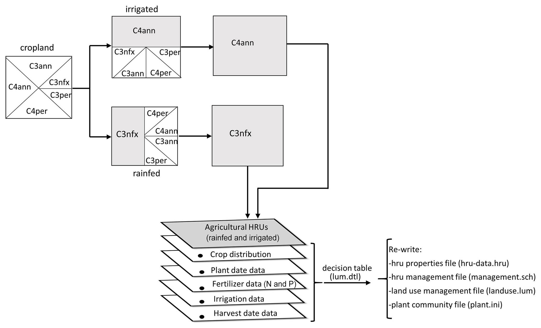
Figure 2Workflow for incorporating crop phenology and crop management data from global datasets into the model.
For both rainfed and irrigated areas, the representative crops with the corresponding crop phenology (plant and harvest dates) and crop management practices (irrigation and N and P fertilizers) were extracted from the respective global datasets (Table 1). The extracted data were written in a decision table for each cropland HRU using a Python code. The default model was rerun with the modified crop scheduling with data from global datasets and is referred to as “revised SWAT+” model from here on.
2.7 Validation of model results
Our study focused on improved cropland use representation. We evaluated our simulations for LAI and ET for a period of 7 years (2009–2015), using the remote sensing products in Table 3. Studies (e.g. Alemayehu et al., 2017; Ha et al., 2018; Nkwasa et al., 2020) have demonstrated the capability of using remote sensing products to evaluate hydrological model outputs.
Representative basins in the model (as shown in Fig. 3) were selected to highlight the importance of incorporating global phenology datasets on LAI simulations in regional hydrological modelling. The selected basins were based on the reported cropping patterns that start with the rainy season (Waha et al., 2013), i.e. the Upper Blue Nile basin with a predominantly single cropping season, the Victoria Basin with a double cropping season, and the Nile Delta with mainly a double irrigated cropping season (Sugita et al., 2017; M. El-Marsafawy et al., 2018). Crop HRUs within the selected subbasins that occupied the largest areas were selected to reduce the effect of mixed LAI from different land cover classes when comparing with the remote sensing LAI.
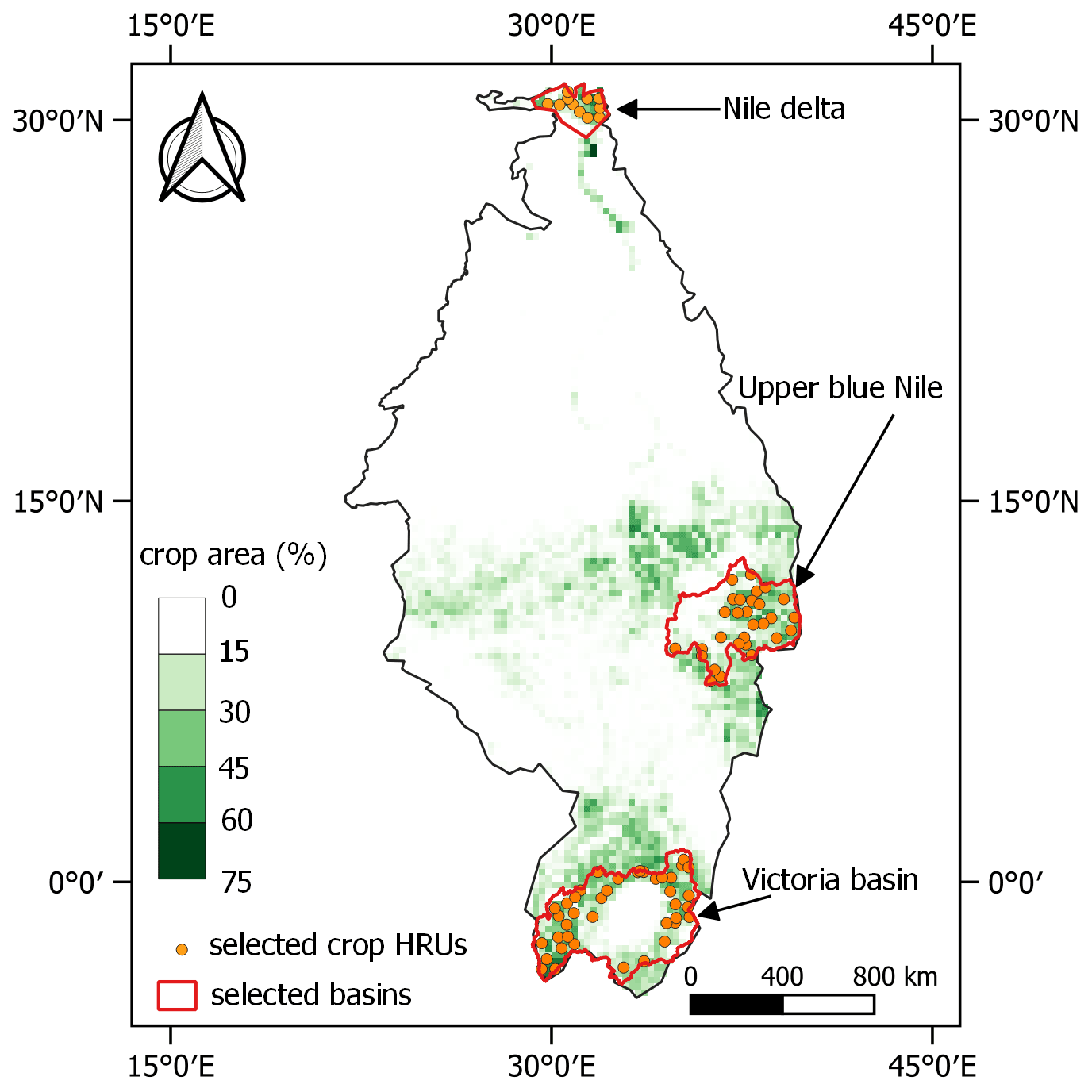
Figure 3Crop area percentage and selected basins for LAI evaluation.
Additionally, the correlation coefficient matrix in Eq. (5) was used for the model evaluation of LAI.
where and are the simulated and observed values at every time step, with and being the respective mean values.
To illustrate the impact of revised cropland use representation on model outputs, we compare the differences in soil erosion simulations between the default and the revised SWAT+ models. However, due to the sparse and poor quality records of erosion and sediment yield in this region (Haregeweyn et al., 2017), it was not possible to quantitatively validate erosion model results. Instead, we adopted a plausibility check approach that is suitable for cases when observations for comparison with model outputs are limited. We compared our erosion estimates for some catchments, e.g. Upper Blue Nile, with those from a few previous studies (Hurni, 1985; Betrie et al., 2011; Haregeweyn et al., 2017). Additionally, the improvement in the representation of crop phenology and crop management practices is expected to minimize errors associated with estimating soil erosion, specifically the crop management factor estimation in the MUSLE.
Both model set-ups were uncalibrated but checked for the water balance. The study targets improving the default model simulations by better representing the physical land processes (crop growth and ET estimation). Thus, default parameterization was used, and we assume that the differences seen in the model set-ups originate primarily from the crop representation and management practices. This approach could not only isolate the uncertainty in the model due to crop representation but also allowed the model results be compared in default parameter conditions, considering that parameter calibrations vary with different catchments. Nkwasa et al. (2020) suggested that improved representation of crop and agricultural land use processes should, in fact, precede any model calibration efforts. Qi et al. (2020) highlighted the importance of improving process representation in a default SWAT model to ensure the reliability of the model in large ungauged basins. Besides, SWAT was developed with the objective of predicting the impact of management on water, sediment, and agricultural yields in large ungauged basins (Arnold et al., 1998; Srinivasan et al., 2010). This paper aims for a better physical representation of the land surface processes of the default model. Hence, we do not address issues concerning the SWAT+ model calibration and validation in this paper.
3.1 Spatiotemporal variability in rainfall for the region
The long-term mean rainfall for 7 years (2009–2015) in the region ranged from 0 to 2200 mm (Fig. 4a). The highest annual rainfall values are recorded around the equatorial region (Victoria Basin) and within parts of Ethiopia (Blue Nile basin). Most arid areas (parts of Egypt) were the driest regions, receiving zero to negligible rainfall within the study period. Figure 4b shows the annual spatiotemporal variation using the coefficient of variation (CV) metric. Interannual variability was highest (CV > 50 %) in the driest region (parts of Egypt) that coincides with the lowest long-term mean rainfall. The rest of the region had low (CV < 20 %) to moderate (20 % < CV < 35 %) interannual variability in rainfall, which means that, in most parts of the region, the total annual rainfall remained relatively stable. A study by Muthoni et al. (2019) in East Africa also reported relatively low interannual variability (<10 %) within the Victoria Basin.
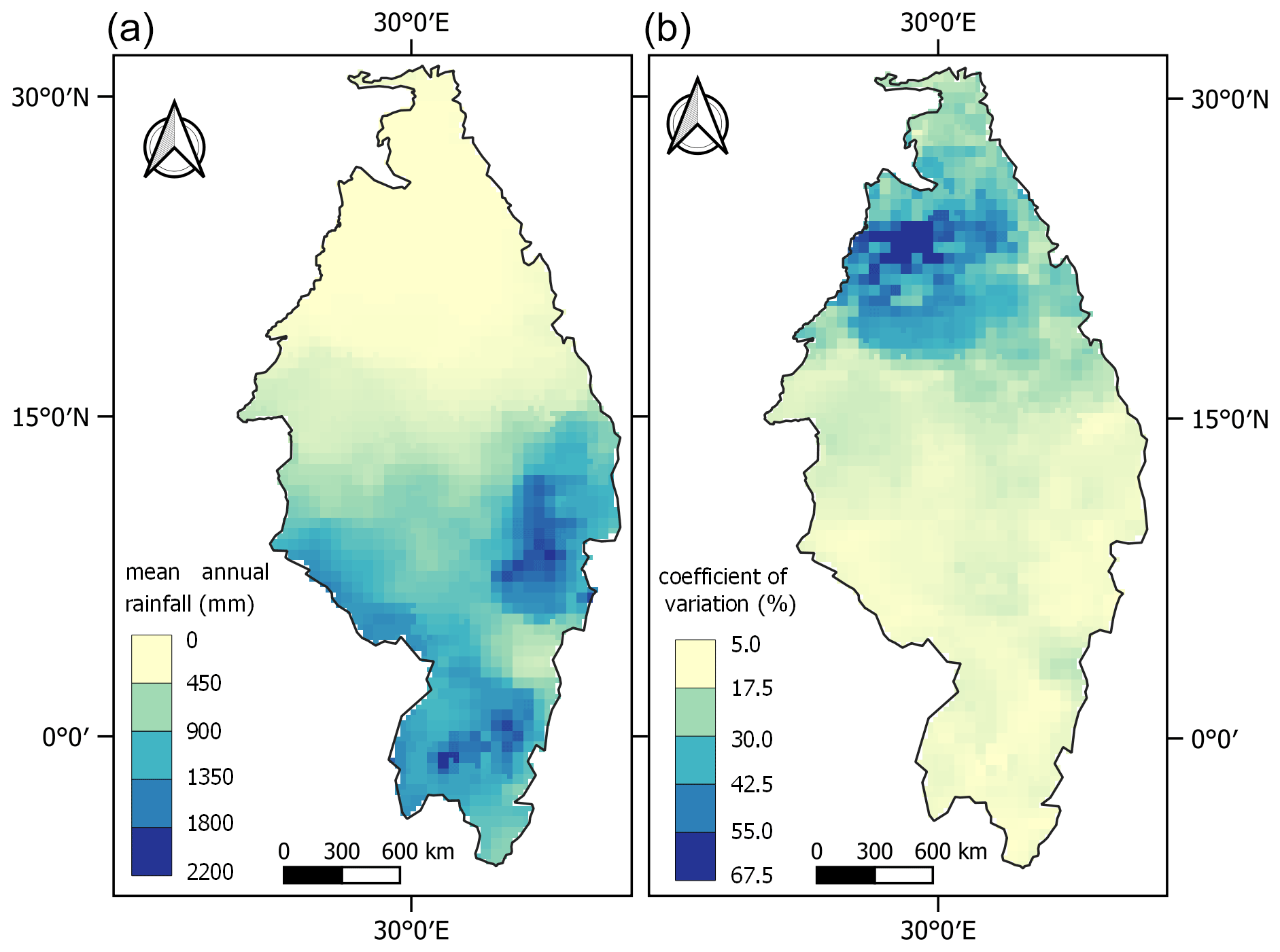
Figure 4(a) Long term mean annual rainfall (2009–2015). (b) Coefficient of variation in annual rainfall.
Figure 5 shows the long-term mean monthly rainfall pattern for selected HRUs in the selected basins (Fig. 3) of the region. The rainfall in the Victoria Basin, located within the equatorial region, exhibits a bimodal pattern with the main wet season in March–May and a short rainy season in October–December. In the Upper Blue Nile basin located within Ethiopia, there is only one main wet season in the months of June–September. For the Nile Delta in Egypt, it is seen that the wet seasons occur in March–May and October–February, with values far lower than the other regions. These monthly patterns are consistent to those indicated by Onyutha and Willems (2015). The wet seasons (start and end of the rainy period) represent the major cropping seasons in the Nile Basin, as rainfall is the primary controlling factor for leafing and senescence in tropical and subtropical regions (Ma et al., 2019).

Figure 5Long-term monthly mean and standard deviation (lines) rainfall pattern for selected HRUs in selected basins within the region.
3.2 LAI simulations
The simulated LAI from both the default and revised SWAT+ models was compared with the remote sensing LAI extracted for the maize, wheat, and soybean HRUs in the three selected subbasins (Upper Blue Nile, Lake Victoria, and Nile Delta). In the Upper Blue basin (Fig. 6a and c), there is an improved LAI simulation in the revised SWAT+ model, with the phenological development being captured in the correct major cropping season within the rainy season for both the rainfed and irrigated maize HRUs. Additionally, the revised SWAT+ model LAI strongly correlates (rd>0.5) with the remote sensing (RS) LAI. Figure A1a and A1c in Appendix A also show the improvement in LAI simulations for rainfed and irrigated wheat HRUs in the Upper Blue Nile basin.
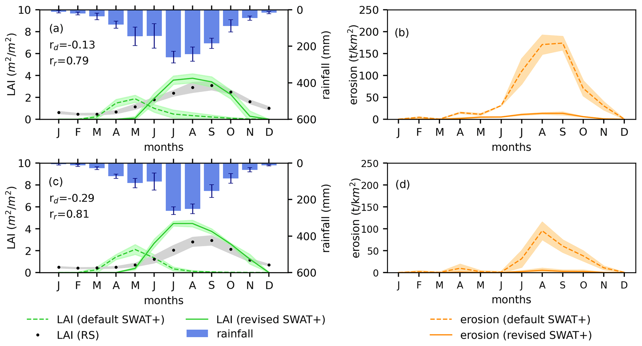
Figure 6Monthly mean and standard deviation (bands) of LAI (a, c) and erosion (b, d) comparison for rainfed maize and irrigated maize, respectively, in the Upper Blue Nile basin. The LAI coefficients (rd are for the default SWAT+ model and rr for the revised SWAT+ model) are shown.
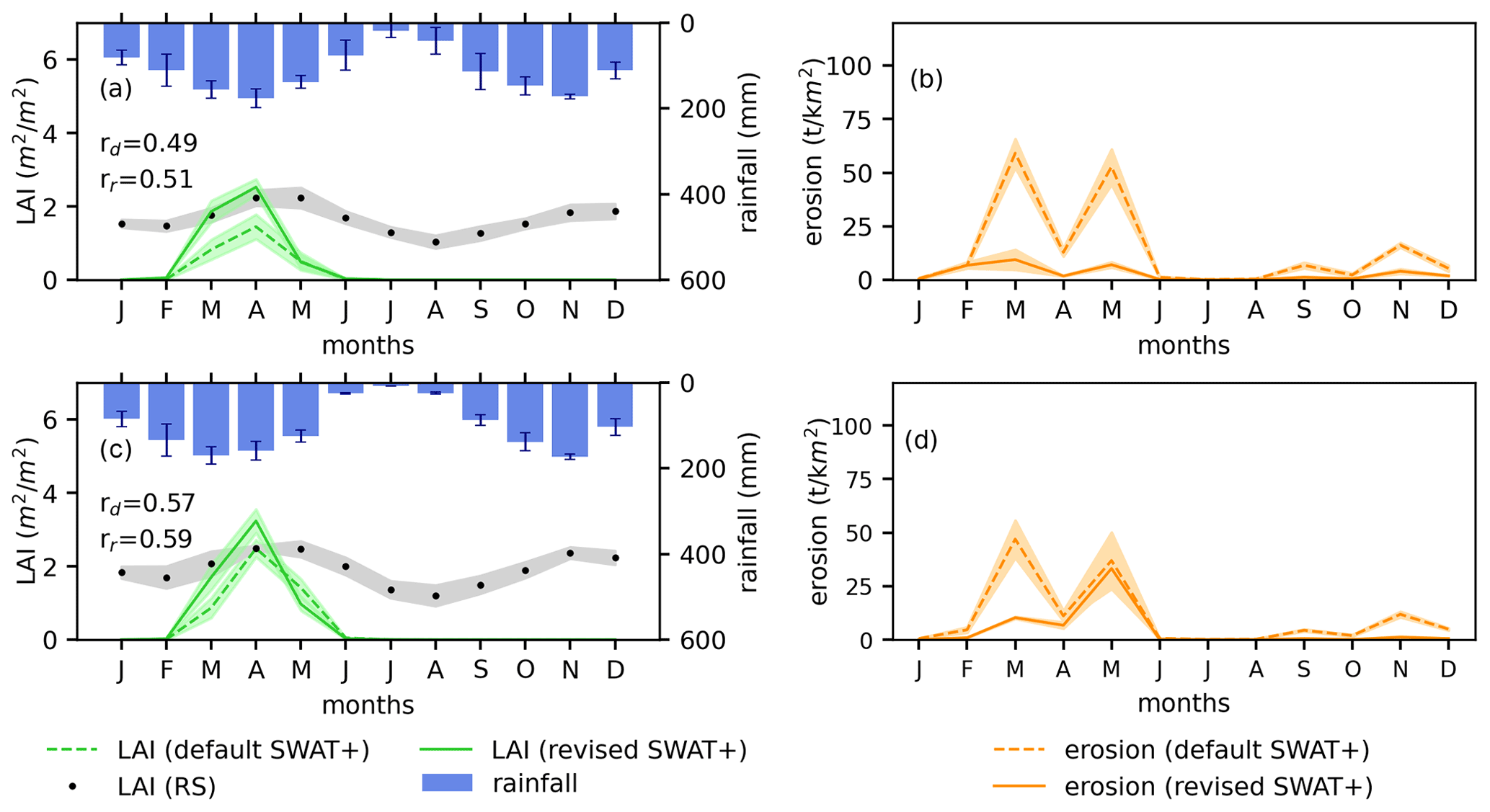
Figure 7Monthly mean and standard deviation (bands) of LAI (a, c) and erosion (b, d) comparison for rainfed wheat and irrigated wheat, respectively, in the Victoria Basin. The LAI correlation coefficients (rd for the default SWAT+ model and rr for the revised SWAT+ model) are shown.
In the Victoria Basin (Fig. 7a and c), the revised SWAT+ model captures only one cropping season in comparison to the RS LAI that shows a double seasonal pattern agreeing with the rainfall. This is because the global dataset (Jägermeyr et al., 2021) utilized captures only the main cropping season per pixel per crop; hence, the model misses the additional cropping seasons. Additionally, Fig. A2a and A2c in Appendix A also show a single cropping season captured in the Victoria Basin for irrigated maize HRUs, with some HRUs having a cropping season from April to November (irrigation in the dry season), while others have a cropping season from September to January (irrigation in the second rainy season). There is also a slight improvement in the LAI correlations for the default and revised SWAT+ models with RS LAI in the Victoria Basin, as the LAIs simulated by the revised SWAT+ model are indicative of the representative crops planted in the basin as compared the generalized crop representation in the default model.

Figure 8Monthly mean and standard deviation (bands) of LAI (a) and erosion (b) comparison for irrigated wheat in the Nile delta. The LAI correlation coefficients (rd for the default SWAT+ model and rr for the revised SWAT+ model) are shown.
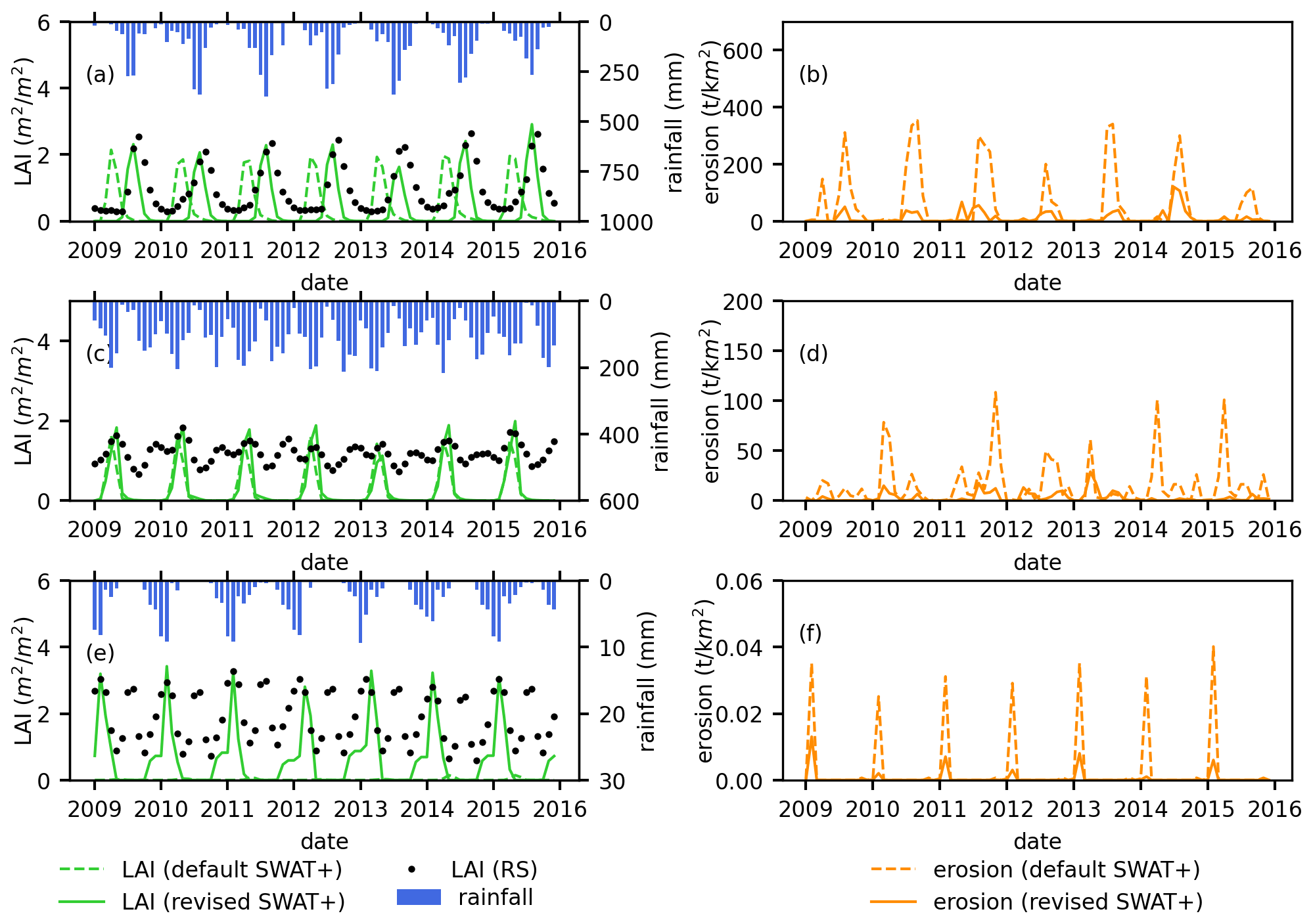
Figure 9(a) Monthly LAI comparison for rainfed maize. (b) Monthly erosion estimates for rainfed maize in the Upper Blue Nile basin. (c) Monthly LAI comparison for rainfed wheat. (d) Monthly erosion estimates for rainfed wheat in the Victoria Basin. (e) Monthly LAI comparison for irrigated wheat. (f) Monthly erosion estimates for irrigated wheat in the Nile Delta.
For the Nile Delta that is predominantly irrigated, the revised SWAT+ model improves the LAI simulations (from to 0.48) as compared to the default SWAT+ model that simulates a negligible LAI (Fig. 8a). Without management practices (irrigation and fertilization), plant growth in the default SWAT+ model is constrained in the Nile Delta, which is a predominantly dry region, resulting in low LAI simulations. However, with the cropping calendar and the associated management practices, LAI simulations are improved in the revised model. The revised SWAT+ model still captures only one cropping season as compared to the RS LAI that shows two cropping seasons that are also highlighted in previous studies (M. El-Marsafawy et al., 2018).
The interannual variability in LAI within the selected basins was also examined for selected crops in Fig. 9, but no significant interannual variations were noticed. This can be explained by the low interannual variability in rainfall for most parts of the region (Fig. 4b) within the study period. However, the seasonal patterns remained consistent, with the LAI peaking in the wet/rainy seasons within all the selected basins. The low interannual variability of the LAI within the study period certainly does not imply that the relevance of the variability in LAI interannually is unimportant in the region, as an analysis on a longer time series could yield different results.
From all the basins, we see an improved seasonal temporal crop growth phenological development pattern with the revised model as compared to the default model for both the rainfed and irrigated regions, which underscores the relevance of the methodological advancements in this paper. However, in the Victoria Basin and the Nile Delta, where we have two dominant cropping seasons, the global datasets still capture one cropping season. Additionally, some regions in East Africa have been reported to have up to three cropping seasons (Waha et al., 2013; Msigwa et al., 2019), which have not been captured in these simulations. The global crop calendars also lack a temporal time series dimension which could be a substantial source of uncertainties in predicting phenological events of croplands. The lack of observational data of multiple cropping seasons at the regional scale has been reported in previous studies (Rounsevell et al., 2003). Some studies (Ma et al., 2019; Rajib et al., 2020) have used remote sensing LAI datasets, e.g. MODIS, to improve LAI simulations with SWAT in tropical subtropical regions. Remote sensing can be useful for the characterization of cropping systems; however, expert judgement and local knowledge is still required for crop type and crop management mapping (Bégué et al., 2018). Combining remote sensing datasets with existing global phenology datasets provides the potential for addressing the gap in multiple cropping datasets. With recent research progress in cropping patterns, such as the crop generator (Sietz et al., 2021) that is used to reproduce crop rotation characteristics at the regional scale, the global phenology datasets can be improved to consider multiple cropping seasons.
The use of remote sensing LAI data (1 km resolution) in the evaluation could also present uncertainties, since the remote sensing data do not represent a pure signal of a crop but rather vegetation with in the pixel. Studies (Ma et al., 2019; Nkwasa et al., 2020) have highlighted these scaling issues when using remote sensing products in model evaluation. Remote sensing pixels are usually presented in a grid system that cannot sufficiently capture the spatial details of mixed vegetation within a grid. Nevertheless, the remote sensing data still provide insights on the temporal vegetation growth relationship with seasonal weather patterns.
3.3 ET simulations
The annual average simulated agricultural ET from the revised SWAT+ model improves the default agricultural ET simulation from 732 to 837 mm yr−1 as compared to the WaPOR agricultural ET of 936 mm yr−1. The improvement in the spatial distribution of the agricultural ET is shown in Fig. 10. Figure 10a and b show the default model simulation and the revised SWAT+ model simulation, respectively, in reference to WaPOR ET (Fig. 10c). The inclusion of the global phenology and management practices shows that ET is one of the major components of a basin water balance that is greatly influenced by the seasonal vegetation growth cycles. This can be attributed to the improved temporal patterns of LAI, which favours transpiration and evaporation from canopy-intercepted water. According to Wang et al. (2014), incorporating LAI and vegetation growing stages in modelling could explain half of the variability in transpiration to ET ratios across ecosystems. Hence, overlooking crop representation in hydrological models is not physically meaningful because a poor simulation of LAI has a cascading effect on how the model partitions the ET fluxes.
Although, the agricultural ET is improved with the incorporation of the global crop phenology, there is still an underestimation, especially in the Nile Delta and the equatorial region (Fig. 10d). This underestimation could be mainly attributed to the missing multiple cropping seasons, especially in areas that are irrigated such as the Nile Delta. As mentioned in the previous section, the phenology datasets give only one cropping season, which misrepresents areas with multiple cropping seasons. Furthermore, automatic irrigation was specified in the model, which applies water from a deep aquifer in all irrigation fields when the water stress is below a specified threshold (0.7) of the field capacity. However, extracting irrigation water from a deep aquifer at all irrigation fields may be unrealistic, causing uncertainties in irrigation applications which affect the ET estimates.
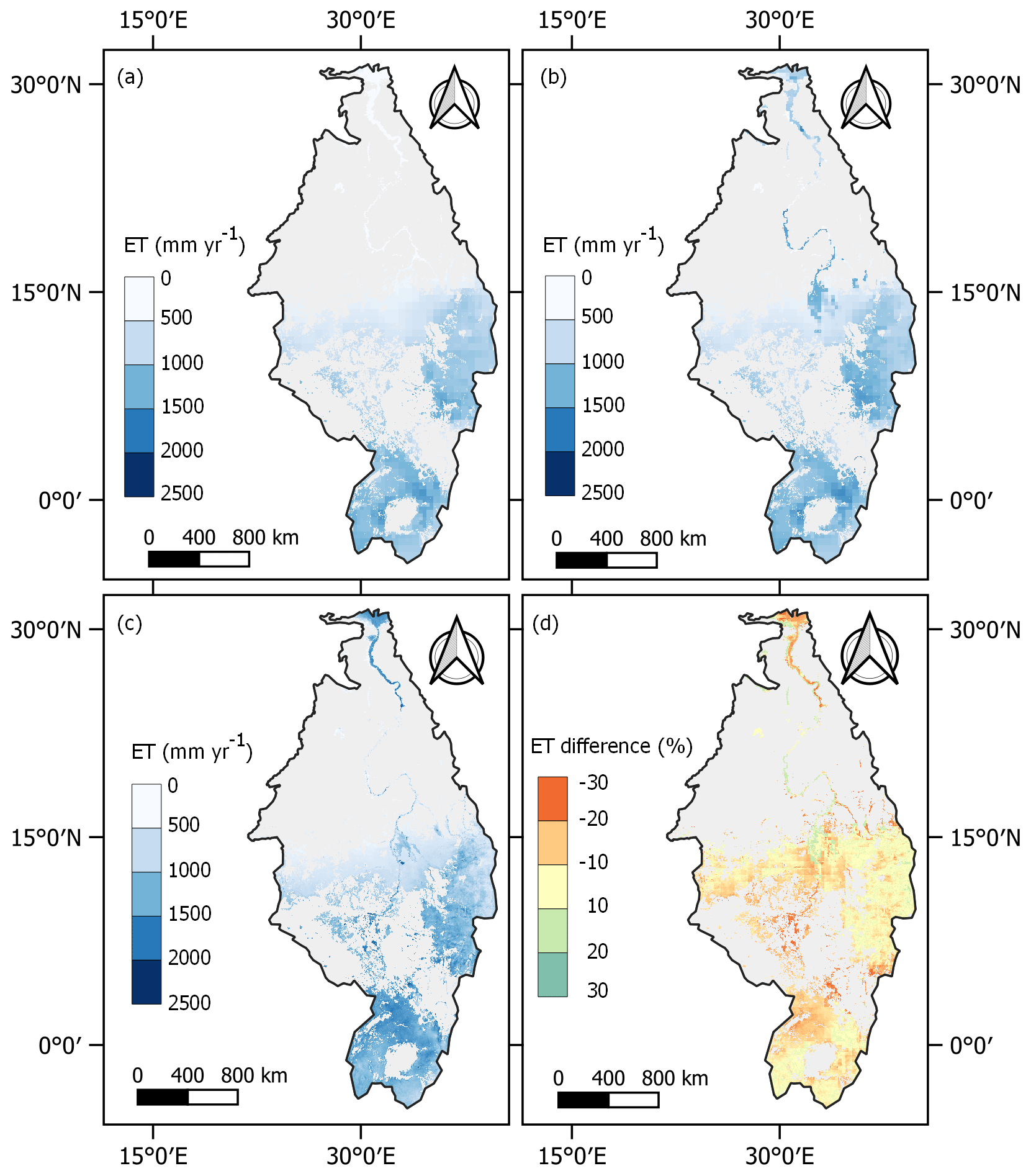
Figure 10Spatial distribution of agricultural ET. (a) Default SWAT+ model ET. (b) Revised SWAT+ model ET. (c) WaPOR ET. (d) ET difference (WaPOR ET − revised SWAT+ model ET).
It is also important to point out that the simplifications made in using a representative crop for the whole pixel could have effects on the ET fluxes due to the simplifications in the variations of the physical characteristics (e.g. LAI, root depth, and stomata conductance) of the heterogenous crops (Burakowski et al., 2018). This simplification can also alter the partitioning of sensible heat fluxes to latent heat fluxes (Eltahir, 1998) that, in turn, affect the ET estimates. Therefore, at local scales, the heterogeneity of crops within a pixel should be considered. The default crop parameterization could also be an extra source of uncertainty in the ET estimates. Although these uncertainties exist, the incorporation of agricultural land use and the corresponding management practices in hydrological models provides a promising way to improve ET estimates especially for cultivated regions. Additionally, the ET estimates could be further improved by model calibrations to obtain the optimal possible ET.
3.4 Erosion simulations
LAI is not only directly related to processes such as rainfall interception, evaporation, transpiration, soil evaporation, and root depth but also to soil erosion through canopy cover, which varies during the growth cycle of the plant. With a better representation of the cropping season, the rainfall season also corresponds with higher LAI values, which results in lower erosion yields.
Figures 6b, d, A1b, A2b, A3d, A4b, and A4d reveal that the soil erosion estimates are reduced in the revised SWAT+ model because the canopy cover grows in the correct cropping season (rainy season), reducing the effective energy of intercepted raindrops. These results conform to a study done by Zhao et al. (2013), which showed a strong correlation in soil erosion reduction with the crop growth cycle. In Fig. 7b and d, even though the cropping season in the revised SWAT+ model captures only one cropping season as the default model, there is still a reduction in the HRU erosion estimates because the revised SWAT+ LAI, which is representative of an actual crop, is greater than the default LAI, which is representative of a generic crop. Hence, we notice that a slight increase in the LAI magnitude has a strong impact on the erosion simulations. Additionally, with a slightly higher LAI magnitude in the revised SWAT+ model, more biomass is generated, which results in more residue that could be more effective in reducing soil erosion even after the cropping season. Residue intercepts rain droplets near the soil surface so that droplets regain no fall velocity. Thus, a given percentage of residue is more effective than the same percentage of canopy cover (Neitsch et al., 2011). However in Fig. 7b and d, the erosion peaks in the default model are strong even though the LAI is relatively high. This can be attributed to the reduction in the residue on the soil surface during the second rainy season that occurs with no crop cover. For the Nile Delta in Fig. 8b, the soil erosion estimates are reduced further, even though they were already insignificant. From Fig. 9b, d and f, it is important to highlight that the low to moderate interannual variability in rainfall (Fig. 4b) for most agricultural areas of the region, coupled with low interannual variation in the simulated LAI shown in Fig. 9a, c and e, resulted in a low interannual variability in erosion simulations.
The average annual soil erosion estimates are reduced by a maximum of 625 t km−2 yr−1 (mostly in the Upper Blue Nile basin; Fig. 11a) or up to 90 % (Fig. 11b) in some areas within the region when using the revised SWAT+ model as compared to the default model. The average regional soil erosion yield reduced by 16 %, with the greatest decrease of 37 % in the Upper Blue Nile basin. This reduction is attributed to the improved timing of the cropping seasons in correspondence to the start of the rainy season, which provides more canopy cover to intercept the raindrops. However, in some isolated regions, the revised SWAT+ model simulated an increase in soil erosion estimates as compared to the default model. In most of those regions, the global phenology data captures the irrigated cropping season, which is often occurring in the dry seasons (Fig. A3a), which causes discrepancies by not representing the major growing season in the rainy season. As mentioned in the previous section, this is attributed to the fact that the global phenology data provide a single cropping season per pixel per year.
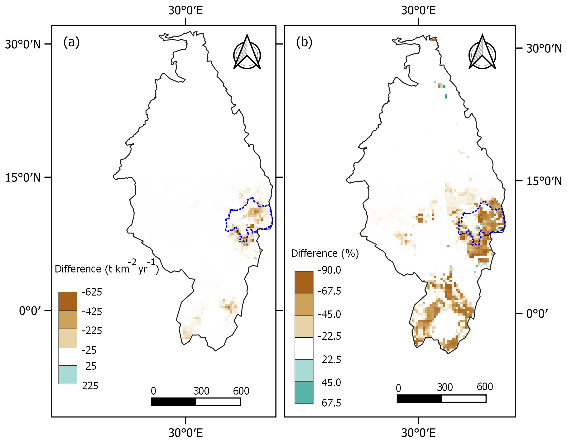
Figure 11Change in erosion estimates (revised SWAT+ model minus default SWAT+ model), with (a) absolute differences and (b) percentage differences.
Among the few hydrological model applications in the subtropics that focus on improved erosion simulations, Ma et al. (2019) enhanced the SWAT model performance by using remotely sensed LAI to give reasonable crop cover estimates, leading to an accurate estimate of soil erosion and sediment yield. However, when using remotely sensed data, detecting crop types and cropping sequences without local knowledge or ground truth data is not possible (Bégué et al., 2018), which emphasizes the importance of the approach proposed in this study.
In order to validate the regional soil erosion estimates, the simulated soil loss from the revised SWAT+ model was compared with the spatial patterns in the erosion rates from the literature. From the published literature, Ethiopia is the one of the most documented countries in northeastern Africa, with marginal information existing for other countries (Haregeweyn et al., 2015). The revised SWAT+ model shows that the regional soil erosion extent varies from 0 to over 20 500 t km−2 yr−1 (Fig. 12), revealing the severity of soil erosion in the Ethiopian highlands as compared to the other parts of the region. The Ethiopian highlands have been reported to have high soil erosion and sediment yield rates, partly attributed to topography and rainfall but also due to recent and historic land conversions to agriculture.

Figure 12Spatial distribution of predicted annual average soil erosion at HRU level in northeastern Africa (2009–2015).
Compared with estimates from the Upper Blue Nile basin, the model estimated an erosion yield extent from 0 to 13 000 t km−2 yr−1 and a mean of 701 t km−2 yr−1, which is slightly lower but comparable to a net soil erosion mean of 734 t km−2 yr−1, as reported by Haregeweyn et al. (2017), and soil erosion yield extents from 0 to over 15 000 t km−2 yr−1, as reported by Hurni (1985), Betrie et al. (2011), and Haregeweyn et al. (2017). Tamene and Le (2015) reported a net soil loss of 8500 and 600 t km−2 yr−1 in the Blue Nile and White Nile basins, respectively. These estimates should be considered as indicative, as comparing these values with the northeastern African regional model estimates can be challenging, mainly due to the differences in the sizes of the areas involved that result from the different delineation procedures.
Even though the regional model underestimates the soil erosion in comparison with these localized studies, the order of magnitude is within the same range. The underestimation can be attributed to the finer resolution of datasets utilized by the local studies as compared to the coarse datasets utilized in the regional model. For example, Molnár and Julien (1998) calculated soil erosion using different digital elevation model (DEM) grid sizes and concluded that the estimated slope gradients decreased as the cell size increased, which influenced the topographic factor (LS) estimation. Additionally, the input global weather data are at a scale of 0.5∘, which makes the data too coarse to capture the spatial variability in weather at a finer scale. This has been a challenge for large-scale hydrological modelling (Chawanda et al., 2020) which needs to be addressed for better performance.
With that background, it is not wise to entirely consider the soil erosion estimates in this study as being an exact quantification but rather as close approximations. It is worth noting that the focus of this study was not soil erosion estimation but to illustrate a concept.
In this work, an approach has been developed for an improved representation of crop phenology and management in a regional SWAT+ model using decision tables and global datasets. In addition, global remote sensing datasets of LAI and ET have been used for model evaluation. A comparison of the simulated LAI revealed improved temporal growth patterns in agreement with remote sensing LAI, especially for regions with a single cropping cycle. However, for regions with multiple cropping cycles, only one cropping cycle was represented, as most global phenology datasets provide a single cropping cycle per year.
The improvements in the SWAT+ model reduced the agricultural ET deficit by 50 % in comparison with the WaPOR ET, showing a strong linkage between hydrological response and agricultural land use representation. Additionally, this improvement in ET estimates is expected to reduce any calibration efforts needed to obtain the maximum possible ET as the physical process representation of crops is improved. A considerable reduction of 16 % in the average regional soil erosion estimates was noticed after implementing this approach. This impact on soil erosion estimates shows the importance of the proper representation of crop processes and is an important element for minimizing errors in soil erosion estimates. These findings emphasize the importance of advancing process representation in physically based models to improve the model reliability.
There is a need for global phenology datasets with multiple cropping seasons for further improvements in the crop representation, especially for improving crop processes in irrigated areas or areas with multiple rainy seasons. For example, mapped global areas of different multiple cropping systems (Waha et al., 2020) can potentially be combined with global phenology datasets to generate a global crop calendar with different cropping systems. The approach developed in this research lays a foundation for improved agricultural land use representation with associated management practices at regional and global scales, which will further improve regional- to large-scale hydrological and water quality impact assessments of global change.
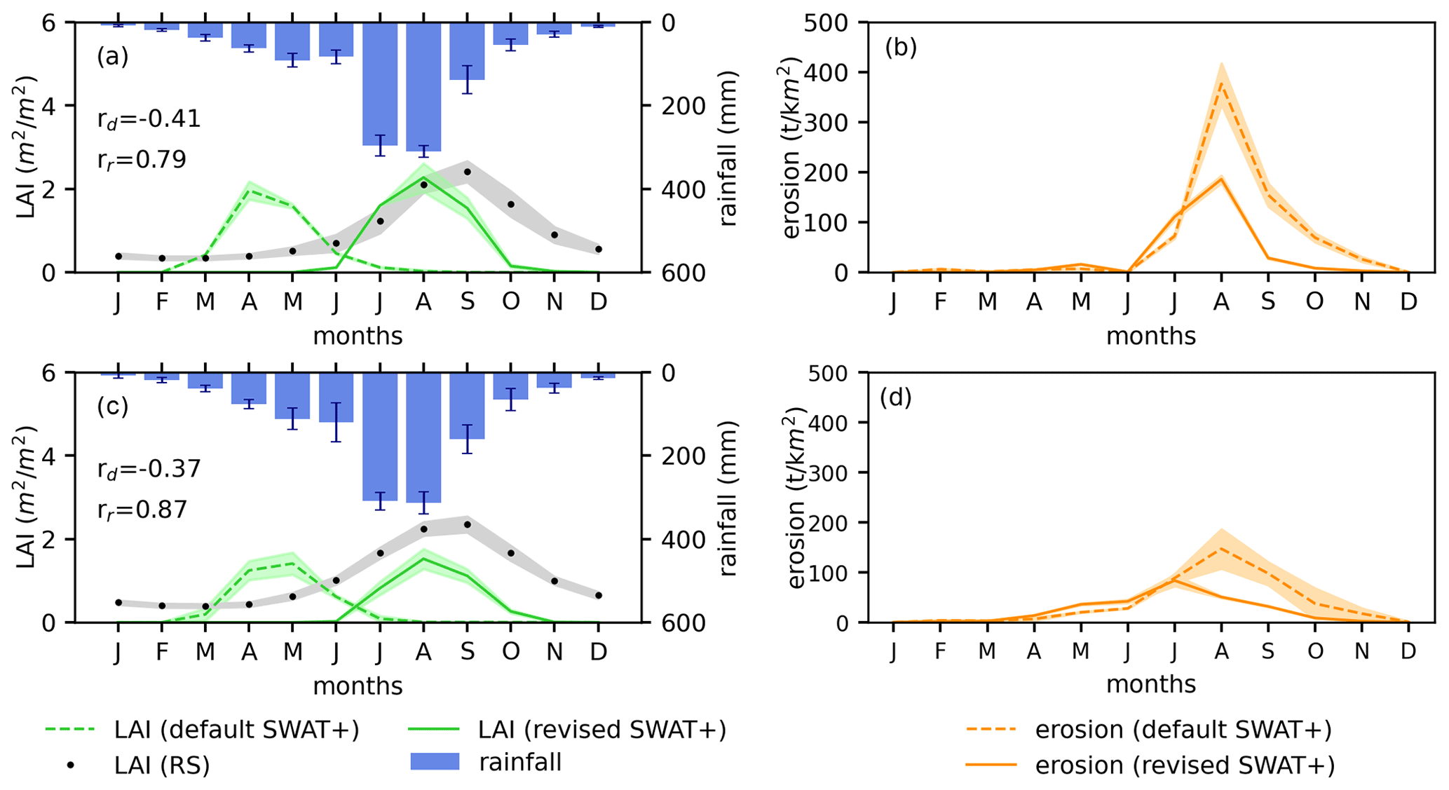
Figure A1Monthly mean and standard deviation (bands) of (a, c) LAI and (b, d) erosion comparison for rainfed wheat and for irrigated wheat, respectively, in the Upper Blue Nile basin. The LAI correlation coefficients (rd for the default SWAT+ model and rr for the revised SWAT+ model) are shown.
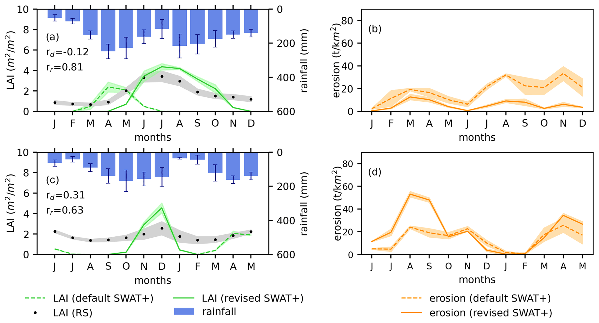
Figure A2Monthly mean and standard deviation (bands) of (a, c) LAI and (b, d) erosion comparison for irrigated maize case 1 (irrigation during the dry growing season) and for irrigated maize case 2 (irrigation during the main wet growing season), respectively, in the Victoria Basin. The LAI correlation coefficients (rd for the default SWAT+ model and rr for the revised SWAT+ model) are shown.

Figure A3Monthly mean and standard deviation (bands) of (a, c) LAI and (b, d) erosion comparison for irrigated soybean case 1 (irrigation during the dry growing season) and for irrigated soybean case 2 (irrigation during the main wet growing season), respectively, in the Victoria Basin. The LAI correlation coefficients (rd for the default SWAT+ model and rr for the revised SWAT+ model) are shown.
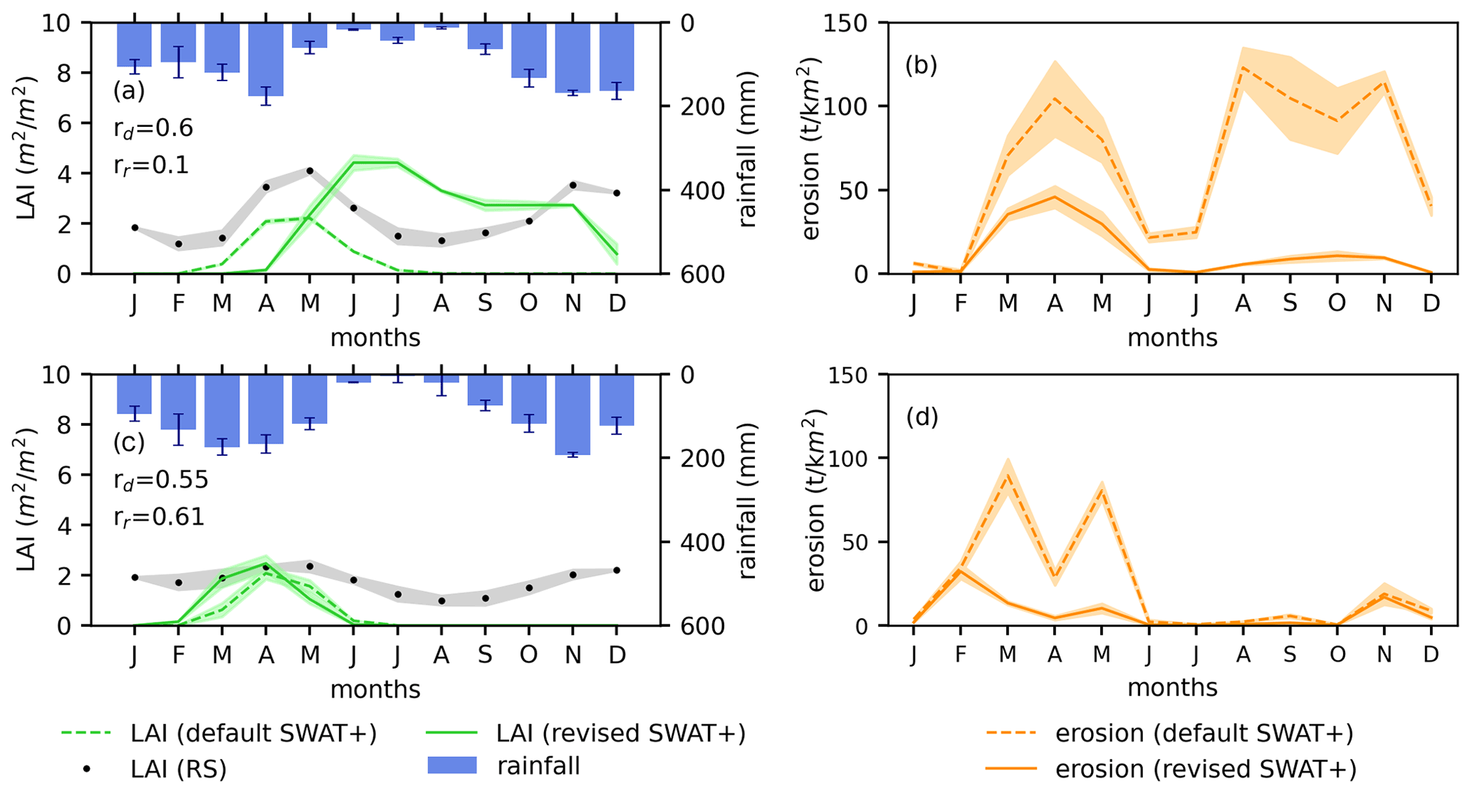
Figure A4Monthly mean and standard deviation (bands) of (a, c) LAI and (b, d) erosion comparison for rainfed maize and for rainfed soybean, respectively, in the Victoria Basin. The LAI correlation coefficients (rd for the default SWAT+ model and rr for the revised SWAT+ model) are shown.
This approach was created using Python scripts available from the VUB-HYDR repository (https://doi.org/10.5281/zenodo.5797553, Nkwasa, 2021). The revisions of the scripts are managed there and are available on request.
The global datasets used in this study are freely available. These include the harmonized land use map (LUH2) from Hurtt et al. (2020; downloadable from https://luh.umd.edu/), the digital elevation model from Farr et al. (2007; downloadable from https://cgiarcsi.community/data/srtm-90m-digital-elevation-database-v4-1/), the soil map from Hengl et al. (2015; downloadable from https://www.isric.org/projects/africa-soil-information-service-afsis), the map of irrigated areas in Siebert et al. (2013; downloadable from https://www.fao.org/aquastat/en/geospatial-information/global-maps-irrigated-areas/latest-version/), the crop phenology dataset from Jägermeyr et al. (2021; downloadable from https://doi.org/10.5281/zenodo.5062513), elemental nitrogen and phosphorus fertilizer maps from Lu and Tian (2017; downloadable from https://doi.org/10.1594/PANGAEA.863323) and Hurtt et al. (2020; downloadable from https://luh.umd.edu/), and observed weather data of rainfall, minimum and maximum temperature, solar radiation, humidity, and wind speed from Lange (2016; downloadable from https://doi.org/10.5880/pik.2016.004). The model outputs are available on request.
AN and AvG designed this study. JJ provided the phenology datasets. CJC and AN set up the model. AN performed the model simulations and primary analysis and drafted the paper. All authors contributed to results interpretation and reviewed the paper.
The contact author has declared that neither they nor their co-authors have any competing interests.
Publisher's note: Copernicus Publications remains neutral with regard to jurisdictional claims in published maps and institutional affiliations.
The authors thank the Research Foundation – Flanders (FWO), for funding the International Coordination Action (ICA) project of “Open Water Network: Open Data and Software tools for water resources management”, the Flemish Research Council (VLIR) for funding the JOINT project of “Global Open Water Academic Network: Joint Research and Education on Open Source Software for Integrated Water Resources Management”, and the EU H2020 programme for funding the project of “Water-ForCE – Water scenarios For Copernicus Exploitation”.
This research has been supported by the Fonds Wetenschappelijk Onderzoek (grant no. G0E2621N), the Vlaamse Interuniversitaire Raad (grant no. TZ2019JOI022A105), and EU H2020 (grant no. 101004186).
This paper was edited by Christian Stamm and reviewed by two anonymous referees.
Abaci, O. and Papanicolaou, A. T.: Long-term effects of management practices on water-driven soil erosion in an intense agricultural sub-watershed: Monitoring and modelling, Hydrol. Process. Int. J., 23, 2818–2837, 2009.
Alemayehu, T., van Griensven, A., and Bauwens, W.: Evaluating CFSR and WATCH Data as Input to SWAT for the Estimation of the Potential Evapotranspiration in a Data-Scarce Eastern-African Catchment, J. Hydrol. Eng., 21, 05015028, https://doi.org/10.1061/(ASCE)HE.1943-5584.0001305, 2016.
Alemayehu, T., van Griensven, A., Woldegiorgis, B. T., and Bauwens, W.: An improved SWAT vegetation growth module and its evaluation for four tropical ecosystems, Hydrol. Earth Syst. Sci., 21, 4449–4467, https://doi.org/10.5194/hess-21-4449-2017, 2017.
Arnold, J., Bieger, K., White, M., Srinivasan, R., Dunbar, J., and Allen, P.: Use of decision tables to simulate management in SWAT+, Water, 10, 713, https://doi.org/10.3390/w10060713, 2018.
Arnold, J. G., Srinivasan, R., Muttiah, R. S., and Williams, J. R.: Large Area Hydrologic Modeling and Assessment Part I: Model Development1, JAWRA J. Am. Water Resour. Assoc., 34, 73–89, https://doi.org/10.1111/j.1752-1688.1998.tb05961.x, 1998.
Arnold, J. G., Moriasi, D. N., Gassman, P. W., Abbaspour, K. C., White, M. J., Srinivasan, R., Santhi, C., Harmel, R. D., Van Griensven, A., and Van Liew, M. W.: SWAT: Model use, calibration, and validation, Trans. ASABE, 55, 1491–1508, 2012.
Arnold, J. G., Kiniry, J. R., Srinivasan, R., Williams, J. R., Haney, E. B., and Neitsch, S. L.: SWAT 2012 input/output documentation, Texas Water Resources Institute, 2013.
Asfaw, A., Simane, B., Hassen, A., and Bantider, A.: Variability and time series trend analysis of rainfall and temperature in northcentral Ethiopia: A case study in Woleka sub-basin, Weather Clim. Extrem., 19, 29–41, https://doi.org/10.1016/j.wace.2017.12.002, 2018.
Bégué, A., Arvor, D., Bellon, B., Betbeder, J., De Abelleyra, D., P. D. Ferraz, R., Lebourgeois, V., Lelong, C., Simões, M., and R. Verón, S.: Remote Sensing and Cropping Practices: A Review, Remote Sens., 10, 99, https://doi.org/10.3390/rs10010099, 2018.
Betrie, G. D., Mohamed, Y. A., van Griensven, A., and Srinivasan, R.: Sediment management modelling in the Blue Nile Basin using SWAT model, Hydrol. Earth Syst. Sci., 15, 807–818, https://doi.org/10.5194/hess-15-807-2011, 2011.
Bieger, K., Arnold, J. G., Rathjens, H., White, M. J., Bosch, D. D., Allen, P. M., Volk, M., and Srinivasan, R.: Introduction to SWAT+, A Completely Restructured Version of the Soil and Water Assessment Tool, JAWRA J. Am. Water Resour. Assoc., 53, 115–130, https://doi.org/10.1111/1752-1688.12482, 2017.
Burakowski, E., Tawfik, A., Ouimette, A., Lepine, L., Novick, K., Ollinger, S., Zarzycki, C., and Bonan, G.: The role of surface roughness, albedo, and Bowen ratio on ecosystem energy balance in the Eastern United States, Agric. For. Meteorol., 249, 367–376, https://doi.org/10.1016/j.agrformet.2017.11.030, 2018.
Camberlin, P.: Nile Basin Climates, in: The Nile: Origin, Environments, Limnology and Human Use, edited by: Dumont, H. J., Springer Netherlands, Dordrecht, 307–333, https://doi.org/10.1007/978-1-4020-9726-3_16, 2009.
Chawanda, C. J., Arnold, J., Thiery, W., and Griensven, A. van: Mass balance calibration and reservoir representations for large-scale hydrological impact studies using SWAT+, Clim. Change, 163, 1307–1327, https://doi.org/10.1007/s10584-020-02924-x, 2020.
Chen, F. and Xie, Z.: Effects of crop growth and development on regional climate: a case study over East Asian monsoon area, Clim. Dyn., 38, 2291–2305, https://doi.org/10.1007/s00382-011-1125-y, 2012.
Eldardiry, H. and Hossain, F.: Understanding Reservoir Operating Rules in the Transboundary Nile River Basin Using Macroscale Hydrologic Modeling with Satellite Measurements, J. Hydrometeorol., 20, 2253–2269, https://doi.org/10.1175/JHM-D-19-0058.1, 2019.
Eltahir, E. A. B.: A Soil Moisture–Rainfall Feedback Mechanism: 1. Theory and observations, Water Resour. Res., 34, 765–776, https://doi.org/10.1029/97WR03499, 1998.
Estel, S., Kuemmerle, T., Levers, C., Baumann, M., and Hostert, P.: Mapping cropland-use intensity across Europe using MODIS NDVI time series, Environ. Res. Lett., 11, 024015, https://doi.org/10.1088/1748-9326/11/2/024015, 2016.
FAO: Using remote sensing in support of solutions to reduce agricultural water productivity gaps, Rome, Italy, available at: https://www.fao.org/3/i7315en/i7315en.pdf (last access: 20 February 2021), 2018.
Farr, T. G., Rosen, P. A., Caro, E., Crippen, R., Duren, R., Hensley, S., Kobrick, M., Paller, M., Rodriguez, E., and Roth, L.: The shuttle radar topography mission, Rev. Geophys., 45, https://doi.org/10.1029/2005RG000183 (data available at: https://cgiarcsi.community/data/srtm-90m-digital-elevation-database-v4-1/, last access: 8 January 2021), 2007.
Fisher, J. B., Melton, F., Middleton, E., Hain, C., Anderson, M., Allen, R., McCabe, M. F., Hook, S., Baldocchi, D., Townsend, P. A., Kilic, A., Tu, K., Miralles, D. D., Perret, J., Lagouarde, J.-P., Waliser, D., Purdy, A. J., French, A., Schimel, D., Famiglietti, J. S., Stephens, G., and Wood, E. F.: The future of evapotranspiration: Global requirements for ecosystem functioning, carbon and climate feedbacks, agricultural management, and water resources, Water Resour. Res., 53, 2618–2626, https://doi.org/10.1002/2016WR020175, 2017.
Gong, T. T., Lei, H. M., Yang, D. W., Jiao, Y., and Yang, H. B.: Effects of vegetation change on evapotranspiration in a semiarid shrubland of the Loess Plateau, China, Hydrol. Earth Syst. Sci. Discuss., 11, 13571–13605, https://doi.org/10.5194/hessd-11-13571-2014, 2014.
Ha, L. T., Bastiaanssen, W. G. M., Van Griensven, A., Van Dijk, A. I. J. M., and Senay, G. B.: Calibration of Spatially Distributed Hydrological Processes and Model Parameters in SWAT Using Remote Sensing Data and an Auto-Calibration Procedure: A Case Study in a Vietnamese River Basin, Water, 10, 212, https://doi.org/10.3390/w10020212, 2018.
Haregeweyn, N., Tsunekawa, A., Nyssen, J., Poesen, J., Tsubo, M., Tsegaye Meshesha, D., Schütt, B., Adgo, E., and Tegegne, F.: Soil erosion and conservation in Ethiopia: A review, Prog. Phys. Geogr. Earth Environ., 39, 750–774, https://doi.org/10.1177/0309133315598725, 2015.
Haregeweyn, N., Tsunekawa, A., Poesen, J., Tsubo, M., Meshesha, D. T., Fenta, A. A., Nyssen, J., and Adgo, E.: Comprehensive assessment of soil erosion risk for better land use planning in river basins: Case study of the Upper Blue Nile River, Sci. Total Environ., 574, 95–108, https://doi.org/10.1016/j.scitotenv.2016.09.019, 2017.
Hengl, T., Heuvelink, G. B. M., Kempen, B., Leenaars, J. G. B., Walsh, M. G., Shepherd, K. D., Sila, A., MacMillan, R. A., Jesus, J. M. de, Tamene, L., and Tondoh, J. E.: Mapping Soil Properties of Africa at 250 m Resolution: Random Forests Significantly Improve Current Predictions, PLOS ONE, 10, e0125814, https://doi.org/10.1371/journal.pone.0125814 (data available at: https://www.isric.org/projects/africa-soil-information-service-afsis, last access: 25 January 2021), 2015.
Hilker, T., Lyapustin, A. I., Tucker, C. J., Hall, F. G., Myneni, R. B., Wang, Y., Bi, J., de Moura, Y. M., and Sellers, P. J.: Vegetation dynamics and rainfall sensitivity of the Amazon, P. Natl. Acad. Sci. USA, 111, 16041–16046, 2014.
Hurni, H.: Erosion-productivity-conservation systems in Ethiopia, Proceedings 4th International Conference on Soil Conservation, Maracay, Venezuela, 654–674, 1985.
Hurtt, G. C., Chini, L., Sahajpal, R., Frolking, S., Bodirsky, B. L., Calvin, K., Doelman, J. C., Fisk, J., Fujimori, S., Klein Goldewijk, K., Hasegawa, T., Havlik, P., Heinimann, A., Humpenöder, F., Jungclaus, J., Kaplan, J. O., Kennedy, J., Krisztin, T., Lawrence, D., Lawrence, P., Ma, L., Mertz, O., Pongratz, J., Popp, A., Poulter, B., Riahi, K., Shevliakova, E., Stehfest, E., Thornton, P., Tubiello, F. N., van Vuuren, D. P., and Zhang, X.: Harmonization of global land use change and management for the period 850–2100 (LUH2) for CMIP6, Geosci. Model Dev., 13, 5425–5464, https://doi.org/10.5194/gmd-13-5425-2020 (data available at: https://luh.umd.edu/, last access: 31 January 2021), 2020.
Iizumi, T., Kim, W., and Nishimori, M.: Modeling the Global Sowing and Harvesting Windows of Major Crops Around the Year 2000, J. Adv. Model. Earth Syst., 11, 99–112, https://doi.org/10.1029/2018MS001477, 2019.
Jägermeyr, J., Müller, C., Ruane, A. C., Elliott, J., Balkovic, J., Castillo, O., Faye, B., Foster, I., Folberth, C., Franke, J. A., Fuchs, K., Guarin, J. R., Heinke, J., Hoogenboom, G., Iizumi, T., Jain, A. K., Kelly, D., Khabarov, N., Lange, S., Lin, T.-S., Liu, W., Mialyk, O., Minoli, S., Moyer, E. J., Okada, M., Phillips, M., Porter, C., Rabin, S. S., Scheer, C., Schneider, J. M., Schyns, J. F., Skalsky, R., Smerald, A., Stella, T., Stephens, H., Webber, H., Zabel, F., and Rosenzweig, C.: Climate impacts on global agriculture emerge earlier in new generation of climate and crop models, Nat. Food, 2, 873–885, https://doi.org/10.1038/s43016-021-00400-y (data available at: https://doi.org/10.5281/zenodo.5062513), 2021.
Lange, S.: EartH2Observe, WFDEI and ERA-Interim data Merged and Bias-corrected for ISIMIP (EWEMBI), GFZ Data Services [data], https://doi.org/10.5880/PIK.2016.004, 2016.
Leff, B., Ramankutty, N., and Foley, J. A.: Geographic distribution of major crops across the world, Glob. Biogeochem. Cycles, 18, GB1009, https://doi.org/10.1029/2003GB002108, 2004.
Li, L., Friedl, M. A., Xin, Q., Gray, J., Pan, Y., and Frolking, S.: Mapping Crop Cycles in China Using MODIS-EVI Time Series, Remote Sens., 6, 2473–2493, https://doi.org/10.3390/rs6032473, 2014.
Lin, J., Zhang, J., Gu, Z., Chen, J., and Lyu, H.: A new approach of assessing soil erosion using the remotely sensed leaf area index and its application in the hilly area, Yegetos, Int. J. Plant Res., 27, 1–12, 2014.
Lokupitiya, E., Denning, S., Paustian, K., Baker, I., Schaefer, K., Verma, S., Meyers, T., Bernacchi, C. J., Suyker, A., and Fischer, M.: Incorporation of crop phenology in Simple Biosphere Model (SiBcrop) to improve land-atmosphere carbon exchanges from croplands, Biogeosciences, 6, 969–986, https://doi.org/10.5194/bg-6-969-2009, 2009.
Lotsch, A., Friedl, M. A., Anderson, B. T., and Tucker, C. J.: Coupled vegetation-precipitation variability observed from satellite and climate records, Geophys. Res. Lett., 30, 1774, https://doi.org/10.1029/2003GL017506, 2003.
Lu, C. and Tian, H.: Global nitrogen and phosphorus fertilizer use for agriculture production in the past half century: shifted hot spots and nutrient imbalance, Earth Syst. Sci. Data, 9, 181–192, https://doi.org/10.5194/essd-9-181-2017 (data available at: https://doi.org/10.1594/PANGAEA.863323), 2017.
M. El-Marsafawy, S., Swelam, A., and Ghanem, A.: Evolution of Crop Water Productivity in the Nile Delta over Three Decades (1985–2015), Water, 10, 1168, https://doi.org/10.3390/w10091168, 2018.
Ma, T., Duan, Z., Li, R., and Song, X.: Enhancing SWAT with remotely sensed LAI for improved modelling of ecohydrological process in subtropics, J. Hydrol., 570, 802–815, https://doi.org/10.1016/j.jhydrol.2019.01.024, 2019.
Makowski, D., Nesme, T., Papy, F., and Doré, T.: Global agronomy, a new field of research. A review, Agron. Sustain. Dev., 34, 293–307, https://doi.org/10.1007/s13593-013-0179-0, 2014.
Metzner, J. R. and Barnes, B. H.: Decision table languages and systems, Academic Press, ISBN 978-1483205366, 2014.
Molnár, D. K. and Julien, P. Y.: Estimation of upland erosion using GIS, Comput. Geosci., 24, 183–192, https://doi.org/10.1016/S0098-3004(97)00100-3, 1998.
Monteith, J. L.: Radiation and crops, Exp. Agric., 1, 241–251, 1965.
Msigwa, A., Komakech, H. C., Verbeiren, B., Salvadore, E., Hessels, T., Weerasinghe, I., and van Griensven, A.: Accounting for Seasonal Land Use Dynamics to Improve Estimation of Agricultural Irrigation Water Withdrawals, Water, 11, 2471, https://doi.org/10.3390/w11122471, 2019.
Mueller, B., Seneviratne, S. I., Jimenez, C., Corti, T., Hirschi, M., Balsamo, G., Ciais, P., Dirmeyer, P., Fisher, J. B., Guo, Z., Jung, M., Maignan, F., McCabe, M. F., Reichle, R., Reichstein, M., Rodell, M., Sheffield, J., Teuling, A. J., Wang, K., Wood, E. F., and Zhang, Y.: Evaluation of global observations-based evapotranspiration datasets and IPCC AR4 simulations, Geophys. Res. Lett., 38, 3–10, https://doi.org/10.1029/2010GL046230, 2011.
Muthoni, F. K., Odongo, V. O., Ochieng, J., Mugalavai, E. M., Mourice, S. K., Hoesche-Zeledon, I., Mwila, M., and Bekunda, M.: Long-term spatial-temporal trends and variability of rainfall over Eastern and Southern Africa, Theor. Appl. Climatol., 137, 1869–1882, https://doi.org/10.1007/s00704-018-2712-1, 2019.
Neitsch, S. L., Arnold, J. G., Kiniry, J. R., Williams, J. R., and King, K. W.: SWAT theoretical documentation, Soil Water Res. Lab. Grassl., 494, 234–235, 2005.
Neitsch, S. L., Arnold, J. G., Kiniry, J. R., and Williams, J. R.: Soil and water assessment tool theoretical documentation version 2009, Texas Water Resources Institute, 2011.
Ngetich, K. F., Mucheru-Muna, M., Mugwe, J. N., Shisanya, C. A., Diels, J., and Mugendi, D. N.: Length of growing season, rainfall temporal distribution, onset and cessation dates in the Kenyan highlands, Agric. For. Meteorol., 188, 24–32, https://doi.org/10.1016/j.agrformet.2013.12.011, 2014.
Nile Basin Initiative: Land use/cover in the Nile Basin – Nile Basin Water Resources Atlas, available at: https://atlas.nilebasin.org/treatise/land-usecover-in-the-nile-basin/ (last access: 8 January 2021), 2016.
Nkwasa, A., Chawanda, C. J., Msigwa, A., Komakech, H. C., Verbeiren, B., and van Griensven, A.: How Can We Represent Seasonal Land Use Dynamics in SWAT and SWAT+ Models for African Cultivated Catchments?, Water, 12, 1541, https://doi.org/10.3390/w12061541, 2020.
Nkwasa, A.: Agricultural land use and crop management implementation in large-scale SWAT+ model applications, Zenodo [code], https://doi.org/10.5281/zenodo.5797553, 2021.
O'Neal, M. R., Nearing, M. A., Vining, R. C., Southworth, J., and Pfeifer, R. A.: Climate change impacts on soil erosion in Midwest United States with changes in crop management, Catena, 61, 165–184, 2005.
Onyutha, C. and Willems, P.: Spatial and temporal variability of rainfall in the Nile Basin, Hydrol. Earth Syst. Sci., 19, 2227–2246, https://doi.org/10.5194/hess-19-2227-2015, 2015.
Portmann, F. T., Siebert, S., and Döll, P.: MIRCA2000 – Global monthly irrigated and rainfed crop areas around the year 2000: A new high-resolution data set for agricultural and hydrological modeling, Glob. Biogeochem. Cycles, 24, GB1011, https://doi.org/10.1029/2008GB003435, 2010.
Potter, P., Ramankutty, N., Bennett, E. M., and Donner, S. D.: Characterizing the spatial patterns of global fertilizer application and manure production, Earth Interact., 14, 1–22, 2010.
Qi, J., Zhang, X., Yang, Q., Srinivasan, R., Arnold, J. G., Li, J., Waldholf, S. T., and Cole, J.: SWAT ungauged: Water quality modeling in the Upper Mississippi River Basin, J. Hydrol., 584, 124601, https://doi.org/10.1016/j.jhydrol.2020.124601, 2020.
Rajib, A., Kim, I. L., Golden, H. E., Lane, C. R., Kumar, S. V., Yu, Z., and Jeyalakshmi, S.: Watershed Modeling with Remotely Sensed Big Data: MODIS Leaf Area Index Improves Hydrology and Water Quality Predictions, Remote Sens., 12, 2148, https://doi.org/10.3390/rs12132148, 2020.
Raymond, P. A., Oh, N.-H., Turner, R. E., and Broussard, W.: Anthropogenically enhanced fluxes of water and carbon from the Mississippi River, Nature, 451, 449–452, https://doi.org/10.1038/nature06505, 2008.
Rounsevell, M. D. A., Annetts, J. E., Audsley, E., Mayr, T., and Reginster, I.: Modelling the spatial distribution of agricultural land use at the regional scale, Agric. Ecosyst. Environ., 95, 465–479, https://doi.org/10.1016/S0167-8809(02)00217-7, 2003.
Schuol, J. and Abbaspour, K. C.: Calibration and uncertainty issues of a hydrological model (SWAT) applied to West Africa, Adv. Geosci., 9, 137–143, 2006.
Schuol, J., Abbaspour, K. C., Yang, H., Srinivasan, R., and Zehnder, A. J. B.: Modeling blue and green water availability in Africa, Water Resour. Res., 44, 1–18, https://doi.org/10.1029/2007WR006609, 2008.
Siad, S. M., Iacobellis, V., Zdruli, P., Gioia, A., Stavi, I., and Hoogenboom, G.: A review of coupled hydrologic and crop growth models, Agric. Water Manag., 224, 105746, https://doi.org/10.1016/j.agwat.2019.105746, 2019.
Siebert, S., Henrich, V., Frenken, K., and Burke, J.: Global map of irrigation areas version 5, Rheinische Friedrich-Wilhelms-Univ. Bonn Ger. Agric. Organ. U. N. Rome Italy, 2, 1299–1327, available at: https://www.fao.org/aquastat/en/geospatial-information/global-maps-irrigated-areas/latest-version/ (last access: 16 February 2021), 2013.
Sietz, D., Conradt, T., Krysanova, V., Hattermann, F. F., and Wechsung, F.: The Crop Generator: Implementing crop rotations to effectively advance eco-hydrological modelling, Agric. Syst., 193, 103183, https://doi.org/10.1016/j.agsy.2021.103183, 2021.
Sood, A. and Smakhtin, V.: Global hydrological models: a review, Hydrol. Sci. J., 60, 549–565, https://doi.org/10.1080/02626667.2014.950580, 2015.
Souza, V. F. C. de, Bertol, I., and Wolschick, N. H.: Effects of soil management practices on water erosion under natural rainfall conditions on a Humic Dystrudept, Rev. Bras. Ciênc. Solo, 41, 1–14, https://doi.org/10.1590/18069657rbcs20160443, 2017.
Srinivasan, R., Zhang, X., and Arnold, J.: SWAT ungauged: hydrological budget and crop yield predictions in the Upper Mississippi River Basin, Trans. ASABE, 53, 1533–1546, 2010.
Srivastava, A., Kumari, N., and Maza, M.: Hydrological Response to Agricultural Land Use Heterogeneity Using Variable Infiltration Capacity Model, Water Resour. Manag., 34, 3779–3794, https://doi.org/10.1007/s11269-020-02630-4, 2020.
Sugita, M., Matsuno, A., El-Kilani, R. M. M., Abdel-Fattah, A., and Mahmoud, M. A.: Crop evapotranspiration in the Nile Delta under different irrigation methods, Hydrol. Sci. J., 62, 1618–1635, https://doi.org/10.1080/02626667.2017.1341631, 2017.
Sundborg, A. and White, W. R.: Sedimentation problems in river basins, France, ISBN 9789231020148, 1982.
Swain, A.: Challenges for water sharing in the Nile basin: changing geo-politics and changing climate, Hydrol. Sci. J., 56, 687–702, https://doi.org/10.1080/02626667.2011.577037, 2011.
Tamene, L. and Le, Q. B.: Estimating soil erosion in sub-Saharan Africa based on landscape similarity mapping and using the revised universal soil loss equation (RUSLE), Nutr. Cycl. Agroecosystems, 102, 17–31, https://doi.org/10.1007/s10705-015-9674-9, 2015.
Twine, T. E., Kucharik, C. J., and Foley, J. A.: Effects of Land Cover Change on the Energy and Water Balance of the Mississippi River Basin, J. Hydrometeorol., 5, 640–655, https://doi.org/10.1175/1525-7541(2004)005<0640:EOLCCO>2.0.CO;2, 2004.
van Griensven, A., Ndomba, P., Yalew, S., and Kilonzo, F.: Critical review of SWAT applications in the upper Nile basin countries, Hydrol. Earth Syst. Sci., 16, 3371–3381, https://doi.org/10.5194/hess-16-3371-2012, 2012.
Viña, A., Gitelson, A. A., Nguy-Robertson, A. L., and Peng, Y.: Comparison of different vegetation indices for the remote assessment of green leaf area index of crops, Remote Sens. Environ., 115, 3468–3478, https://doi.org/10.1016/j.rse.2011.08.010, 2011.
Waha, K., Müller, C., Bondeau, A., Dietrich, J. P., Kurukulasuriya, P., Heinke, J., and Lotze-Campen, H.: Adaptation to climate change through the choice of cropping system and sowing date in sub-Saharan Africa, Glob. Environ. Change, 23, 130–143, https://doi.org/10.1016/j.gloenvcha.2012.11.001, 2013.
Waha, K., Dietrich, J. P., Portmann, F. T., Siebert, S., Thornton, P. K., Bondeau, A., and Herrero, M.: Multiple cropping systems of the world and the potential for increasing cropping intensity, Glob. Environ. Change, 64, 102131, https://doi.org/10.1016/j.gloenvcha.2020.102131, 2020.
Wang, L., Good, S. P., and Caylor, K. K.: Global synthesis of vegetation control on evapotranspiration partitioning, Geophys. Res. Lett., 41, 6753–6757, https://doi.org/10.1002/2014GL061439, 2014.
Williams, J. R. and Berndt, H. D.: Sediment yield prediction based on watershed hydrology, Trans. ASAE, 20, 1100–1104, 1977.
Williams, J. R. and Singh, V.: The EPIC Model, Computer models of watershed hydrology, Water Resour. Publ. Highl. Ranch Colo., 909–1000, 1995.
Xiong, J., Thenkabail, P. S., Gumma, M. K., Teluguntla, P., Poehnelt, J., Congalton, R. G., Yadav, K., and Thau, D.: Automated cropland mapping of continental Africa using Google Earth Engine cloud computing, ISPRS J. Photogramm. Remote Sens., 126, 225–244, https://doi.org/10.1016/j.isprsjprs.2017.01.019, 2017.
Yin, X. and Struik, P. C.: C3 and C4 photosynthesis models: An overview from the perspective of crop modelling, NJAS – Wagening. J. Life Sci., 57, 27–38, https://doi.org/10.1016/j.njas.2009.07.001, 2009.
Zhang, X., Friedl, M. A., Schaaf, C. B., Strahler, A. H., and Liu, Z.: Monitoring the response of vegetation phenology to precipitation in Africa by coupling MODIS and TRMM instruments, J. Geophys. Res.-Atmos., 110, D12103, https://doi.org/10.1029/2004JD005263, 2005.
Zhang, Y., Wu, Z., Singh, V. P., He, H., He, J., Yin, H., and Zhang, Y.: Coupled hydrology-crop growth model incorporating an improved evapotranspiration module, Agric. Water Manag., 246, 106691, https://doi.org/10.1016/j.agwat.2020.106691, 2021.
Zhao, W., Fu, B., and Qiu, Y.: An Upscaling Method for Cover-Management Factor and Its Application in the Loess Plateau of China, Int. J. Environ. Res. Public. Health, 10, 4752–4766, https://doi.org/10.3390/ijerph10104752, 2013.