Poor correlation between large-scale environmental flow violations and freshwater biodiversity: implications for water resource management and the freshwater planetary boundary

The freshwater ecosystems around the world are degrading, such that maintaining environmental flow¹ (EF) in river networks is critical to their preservation. The relationship between streamflow alterations (subsequent EF violations²) and the freshwater biodiversity response is well established at the scale of stream reaches or small basins ($\sim <\mathrm{100}$ km²). However, it is unclear if this relationship is robust at larger scales, even though there are large-scale initiatives to legalize the EF requirement. Moreover, EFs have been used in assessing a planetary boundary³ for freshwater. Therefore, this study intends to conduct an exploratory evaluation of the relationship between EF violation and freshwater biodiversity at globally aggregated scales and for freshwater ecoregions. Four EF violation indices (severity, frequency, probability of shifting to a violated state, and probability of staying violated) and seven independent freshwater biodiversity indicators (calculated from observed biota data) were used for correlation analysis. No statistically significant negative relationship between EF violation and freshwater biodiversity was found at global or ecoregion scales. These findings imply the need for a holistic bio-geo-hydro-physical approach in determining the environmental flows. While our results thus suggest that streamflow and EF may not be the only determinant of freshwater biodiversity at large scales, they do not preclude the existence of relationships at smaller scales or with more holistic EF methods (e.g., including water temperature, water quality, intermittency, connectivity, etc.) or with other biodiversity data or metrics.

1 Introduction

Water resources are inarguably one of the most important natural resources in the Earth system for sustaining life. Nevertheless, these resources and their associated ecosystems are threatened by human actions (Bélanger and Pilling, 2019; Clausen and York, 2008; Vörösmarty et al., 2010; Wilting et al., 2017). Global freshwater covers up to 0.8 % of the total Earth's surface (Gleick, 1996) and inhabits 6 % of all the known species in the world, including 40 % of the total fish diversity and nearly one-third of all vertebrates (Lundberg et al., 2000). Since freshwater ecosystems have high species richness in a relatively small area and are exposed to a high level of pressure, they are more vulnerable to environmental change and human actions than any other ecosystems (Dudgeon et al., 2006). The rapid increase in the demand for natural resources is the fundamental cause of freshwater ecosystem degradation (Darwall et al., 2018). Anthropogenic climate change (Allan and Flecker, 1993; Darwall and Freyhof, 2016; Knouft and Ficklin, 2017; Meyer et al., 1999), overexploitation (Allan et al., 2005), water pollution (Albert et al., 2021; Dudgeon et al., 2006; Reid et al., 2019; Smith, 2003), flow alteration (Nilsson et al., 2005; Vörösmarty et al., 2000), habitat destruction (Dudgeon, 2002), and the introduction of alien species (Gozlan et al., 2010; Vitule et al., 2009) are some of the manifestations of this increased demand which directly threatens freshwater ecosystems. In addition, increased water impoundment in large dams and reservoirs has also led to an array of adversities for freshwater ecosystems, ranging from habitat destruction to irregular flow alterations (Bergkamp et al., 2000). This situation is aggravated by increasing pressure on related Earth system functions, such as climate change and nutrient cycles, which are articulated by their respective transgressions in the planetary boundaries framework (Dudgeon, 2010). Freshwater ecosystem processes that were previously governed by natural Earth system facets such as temperature, rainfall, and relief are now increasingly driven by demographic, social, and economic drivers (Clausen and York, 2008; Kabat et al., 2004; Tyson et al., 2002; Vitousek et al., 1997; Vörösmarty et al., 1997). Freshwater ecosystem health comprises both biotic factors such as biodiversity and abiotic factors such as habitat integrity. As any disruption in the abiotic factors is most likely to be reflected in the biotic status of the freshwater ecosystem, the scope of this paper is confined to the biotic dimension of the freshwater ecosystem (i.e., biodiversity) and not the health of the entire ecosystem.

There has been an increased recognition in recent decades of the need to maintain a natural flow regime in streams to sustain healthy ecosystems (Horne et al., 2017; Poff et al., 1997, 2017; Tickner et al., 2020; Tonkin et al., 2021). Despite the indispensable role of aquatic biodiversity in maintaining the quality of the system (Darwall et al., 2018), the inclusion of such environmental flow (EF) in water management is often controversial, particularly in regions where freshwater availability is limited and is already a matter of severe competition. These competitions have led to an increasing trend for EF violation (insufficient streamflow compared to the recommended EF requirement; see Sect. 2.1 for more details) in the past decade in terms of both severity and frequency (Virkki et al., 2022). This wake-up call has led to several international and national efforts to legalize EF requirements through large-scale EF management schemes (Arthington and Pusey, 2003; Richter et al., 1997, 2003). The Water and Nature Initiative (Smith and Cartin, 2011), the Brisbane Declaration (Brisbane Declaration, 2007), and the Global Action Agenda (Arthington et al., 2018) are some of these efforts. Nevertheless, there is a large gap in our understanding of the relationship between EF requirements and biodiversity responses at various spatial and temporal scales. Except for a few (Domisch et al., 2017; Xenopoulos et al., 2005; Yoshikawa et al., 2014), the majority of the studies exploring this relation were conducted at smaller scales (Anderson et al., 2006; Arthington and Pusey, 2003; Powell et al., 2008). Thus, there is a significant discrepancy in the scale at which these processes are understood versus the scale at which the policies are set (Thompson and Lake, 2010). Current knowledge of how the small-scale processes scale up (e.g., validation of large-scale EF hydrologic methods using local data) to a regional or global scale is thus limited, potentially undermining the scientific integrity of existing large-scale EF management schemes.

In order to scientifically underpin large-scale EF policies, the existing assumption of the inverse relationship between freshwater biodiversity response and EF violation must be tested at regional and global scales (see Sect. S1 in the Supplement for more details). Therefore, in this study, we evaluate the relationship between EF violation and freshwater biodiversity at two different spatial scales (freshwater ecoregion and global) using four EF violation indices (frequency, severity, probability of moving to a violated state, and probability of staying violated) and seven freshwater biodiversity indicators describing taxonomic, functional, and phylogenetic dimensions of the biodiversity. The paper is not intended to be a definitive test of the relationship between EF violation and aquatic biodiversity. It is rather intended to be an exploratory analysis of the idea of conducting more detailed evaluations of the EF–biodiversity relationship before formulating large-scale EF management policies. The implications of the findings for large-scale water management and the use of the relationship between environmental flows and freshwater biodiversity (hereafter referred to as the EF–biodiversity relationship) in the planetary boundary framework are also discussed. Introduction to the blue water planetary boundary framework. The planetary boundaries framework proposed by Rockström et al. (2009) and further developed by Steffen et al. (2015) defines planetary-scale biogeophysical boundaries for Earth system processes that, if violated, can irretrievably impair the Holocene-like stability of the Earth system. The framework establishes scientifically determined safe operating limits for human perturbations through control and response variable relationships, under which humans and other life forms will coexist in equilibrium without jeopardizing the Earth's resilience. Nine planetary boundaries were defined to cover all independent significant Earth system processes. Out of those nine, the freshwater planetary boundary quantifies the safe limits of the terrestrial hydrosphere (Gleeson et al., 2020a, b). The freshwater planetary boundary was originally defined using human water consumption as the control variable, set at 4000 km³ yr⁻¹ (with an uncertainty of 4000 to 6000 km³ yr⁻¹) (Rockström et al., 2009). Gerten et al. (2013) proposed a bottom-up, spatially explicit quantification of EF violations as part of the water boundary, while Gleeson et al. (2020b) subdivided the water planetary boundary into six sub-boundaries and proposed possible control and response variables for each, with aquatic biosphere integrity (i.e., EF) as the potential control variable for a surface water sub-boundary. Quantitative evaluation of the strength and scalability of the identified control and response variables is still required.

2 Methodology and data

The study was conducted at two spatially aggregated scales, (1) global and (2) ecoregion, for a historic time period of 30 years (1976–2005). All the underlying calculations were done at level 5 HydroBASIN (median basin area = 19 600 km²) (Lehner and Grill, 2013) and were aggregated to the corresponding spatial scale for further analysis. Level 5 HydroBASIN (also referred to as “basin” in this paper) was selected as the smallest spatial unit as it is the highest level of specificity that can be rasterized into a 0.5^∘ resolution grid without significantly reducing the number of sub-basins smaller than a grid cell (Virkki et al., 2022). The EF violation indices were calculated using the novel environmental flow envelope (EFE) framework of Virkki et al. (2022), and biodiversity was represented by a combination of relative and absolute value indices. The overall workflow for this manuscript is depicted in Fig. 1.

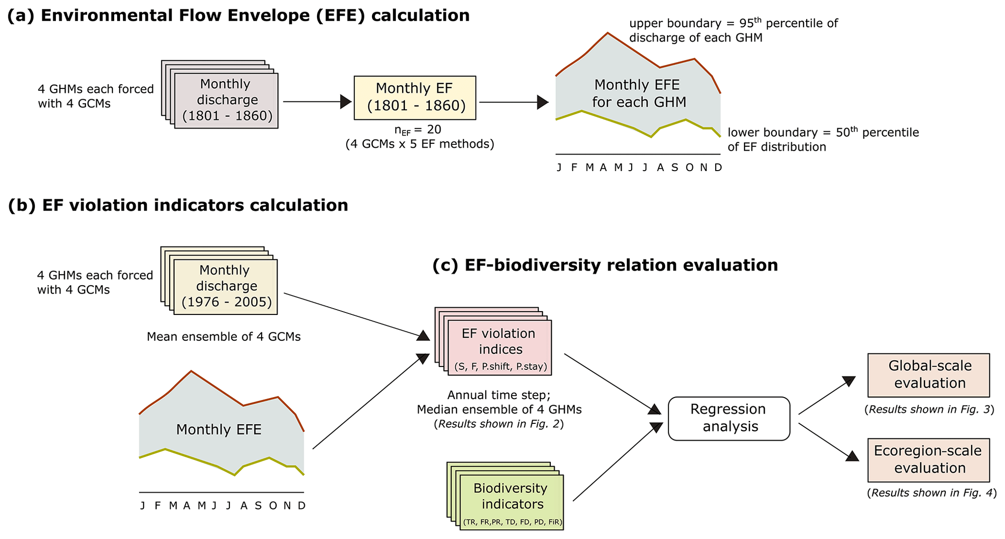
Figure 1 Outline of the methodologies used for (a, b) EF violation indicator calculation and (c) EF–biodiversity relationship evaluation.

2.1 Data

2.1.1 Streamflow data

Streamflow data used in the EFE (see Sect. 2.2 for more details) definition were obtained from the Inter-Sectoral Impact Model Intercomparison Project (ISIMIP) simulation phase 2b outputs of global daily discharge (available at https://esg.pik-potsdam.de, last access: 27 January 2021) (Warszawski et al., 2014). Monthly streamflow data (averaged from the daily simulations) for two time periods were used in this study: (1) data for the pre-industrial era (1800–1860), which was considered the unaltered reference period (Poff et al., 1997), and (2) data for the recent time period (1976–2005). These monthly streamflow datasets were used to calculate EF violations. To calculate the EF violation indices, the estimated EFEs for each basin were obtained from Virkki et al. (2022). A total of four global hydrological models (GHMs) (H08 – Hanasaki et al., 2018; LPJmL – Schaphoff et al., 2018; PCR-GLOBWB – Sutanudjaja et al., 2018; WaterGAP2 – Müller Schmied et al., 2016) were used to obtain the monthly streamflow data. Each GHM was forced with the outputs from four different global circulation models (GCMs) (GFDL-ESM2M – Dunne et al., 2012; HadGEM2-ES – Collins et al., 2011; The HadGEM2 Development Team, 2011; IPSL-CM5A-LR – Dufresne et al., 2013; MICROC5 – Watanabe et al., 2010). All the GHM outputs used in this study were extensively validated and evaluated in several previous studies (e.g., Zaherpour et al., 2018; Gädeke et al., 2020). Moreover, as part of the ISIMIP impact model intercomparison activity, all the GCM climate input data were bias corrected using compiled reference datasets covering the entire globe at 0.5^∘ resolution (Frieler et al., 2017). Additionally, the GHM outputs were also validated using historical data to better fit reality (Frieler et al., 2017). Therefore, no additional volition of the data was done in this study.

The streamflow data were aggregated to the sub-basin scale according to level 5 HydroBASIN version 1.0 (https://www.hydrosheds.org/page/hydrobasins, last access: 27 January 2021) (Lehner and Grill, 2013). The data from ISIMIP 2b are representative of historical land use and other human influences, including dams and reservoirs (Frieler et al., 2017). The maximum discharge cell value within the boundaries of each level 5 HydroBASIN was chosen to represent the outlet discharge value. Any violations within the outlet cell were regarded as indicative of the entire basin, even if conditions could differ in various areas within the level 5 HydroBASIN. As the spatial resolution of the study was level 5 HydroBASIN to allow a global analysis, we accept a certain homogenization of the local-scale characteristics. See Sect. S2 of the Supplement for more details on the datasets used in this study.

2.1.2 Freshwater biodiversity data

In addition to the streamflow data, data on fish diversity were also used in this study (Table 1). Freshwater biodiversity was evaluated using seven indices estimated from the observed biota data. The biodiversity indicators were obtained from international agencies and the literature. The biodiversity indicators consisted of six indices of relative change in biodiversity and one index of the absolute value of biodiversity.

Table 1 Details of the different data used in this study.

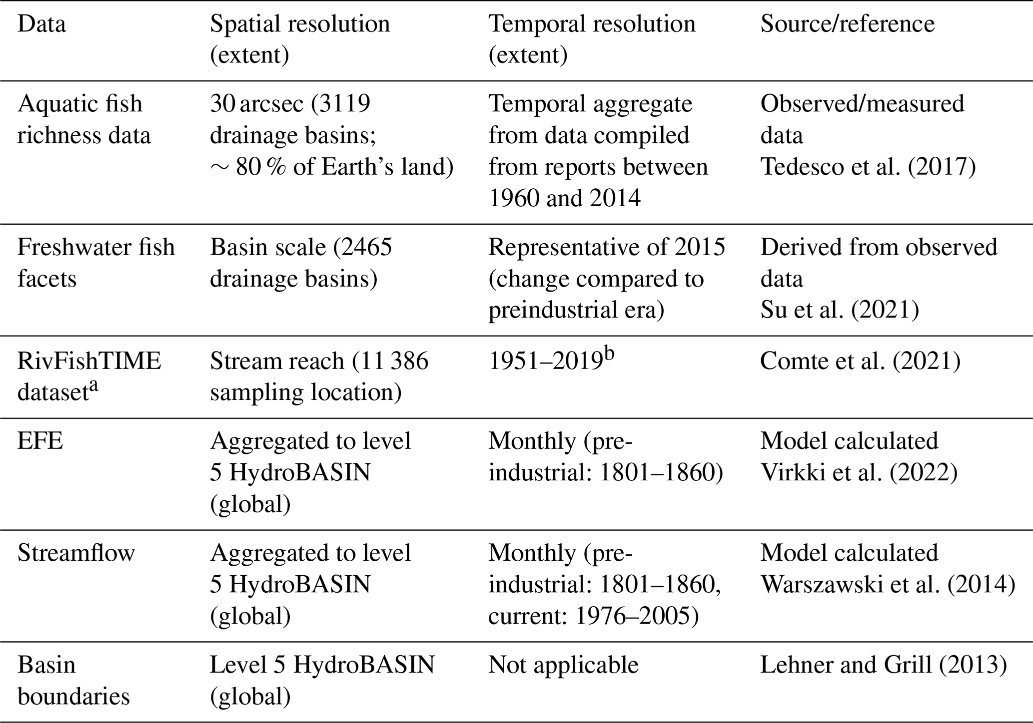
^a Results are only shown in the Supplement (see Sect. S8). ^b Variable for each species and sampling site. Each time series has a minimum survey length of 2 years (mean = 8 years).

(a) Absolute biodiversity indicator

The absolute biodiversity indicator consisted of freshwater fish richness (FiR). The fish richness data were compiled and processed from 1436 published papers, books, gray literature, and web-based sources published between 1960 and 2014 (Tedesco et al., 2017). They cover 3119 basins all over the world and account for 14 953 fish species permanently or occasionally inhabiting freshwater systems. In addition to FiR, we used the RivFishTIME dataset by Comte et al. (2021) – compiled from long-term riverine fish surveys from 46 regional and national monitoring programmes and from individual academic research efforts. Though the RivFishTIME dataset is highly spatially skewed towards the already data-rich regions of Europe, North America (particularly the United States of America) and Australia and is temporally discontinuous, it is the only species-specific fish abundance time series data available and it is useful to have an independent verification of the findings using FiR and relative biodiversity indicators.

(b) Relative biodiversity indicators

The relative biodiversity indicators consisted of six freshwater fish facets. Six key facets of freshwater fish – taxonomic, functional, and phylogenetic diversity (TR, FR, and PR, respectively) as well as the dissimilarity of each of the three groups (TD, FD, and PD, respectively) – were used in this analysis to construct a holistic picture of the state of aquatic biodiversity (see Fig. 1 in Su et al., 2021 for more details on fish facet calculations). Each facet indicates the change in the corresponding biodiversity component compared to the 18th century (roughly the pre-industrial era). The taxonomic facets measure the occurrence of fish in a riverine system. Functional facets are calculated using the morphological characteristics of each species that are linked to feeding and locomotive functions, which in turn relate to larger ecosystem functions such as food web control and nutrition transport. Phylogenetic facets measure the total length of branches linking all species from the assemblage on the phylogenetic tree. The richness component of the three categories calculates the diversity among the assemblage, whereas the dissimilarity accounts for the difference between each pair of fish assemblages in one realm. All six fish facets were calculated at basin scale (2465 river basins), covering 10 682 fish species all over the world. The scale at which the fish facets are estimated does not necessarily align with the scale at which the EF violations are estimated in all cases. The basin-scale facet estimates were then matched with corresponding EF violation indices using different aggregation/data-matching methods (see Sect. 2.4 for more details). All six facets are available as a single delta change in time and do not cover multiple time steps.

2.2 Environmental flow violation estimation

The EFE framework proposed by Virkki et al. (2022) was used to evaluate EF violations in this study. The EFE framework establishes an envelope of variability constrained by discharge limits beyond which flow in the streams may not meet freshwater biodiversity needs (Virkki et al., 2022). EFE uses the pre-industrial (1801–1860) stream discharge to establish an upper and a lower boundary for EF deviations at monthly time steps. This EFE is used to define the EF violation at the level 5 HydroBASIN scale. The EF violations were calculated as the median ensemble of four global hydrological models (GHMs) (H08, LPJmL, PCR-GLOBWB, WaterGAP2) and the mean ensemble of four global circulation models (GCM) (GFDL-ESM2M, HadGEM2-ES, IPSL-CM5A-LR, MICROC5). Moreover, five different EF calculation methods – the Smakhtin method (Smakhtin et al., 2004), the Tennant method (Tennant, 1976), Q90–Q50 (Pastor et al., 2014), the Tessmann method (Tessmann, 1979), and the variable monthly flow method (Pastor et al., 2014)) were also used in the EFE derivation (see Table S3 for more information on EF methods) (Virkki et al., 2022). This approach addresses the uncertainty related to the outputs of models and may eliminate the largest model-related extremes that might cause results to be distorted (Virkki et al., 2022). In spite of the uncertainty in hydrological estimates generated by using different models, a simple ensemble matrix often produces acceptable discharge at larger scales as the individual model bias is removed (Zaherpour et al., 2018). Moreover, all the basins with mean annual flow (MAF) < 10 m³ s⁻¹ were excluded due to high uncertainty in EFE and streamflow estimates (Gleeson et al., 2020a; Steffen et al., 2015; Virkki et al., 2022). After this exclusion, a total of 3906 basins were considered for further analysis. However, many low flows are seasonally observed, such that the MAF may be quite large due to elevated wet season flows, with extremely low flows occurring during a dry season (e.g., Eel River Basin, California), making it difficult to model. In such cases with higher intra-annual flow variability, it is appropriate to consider more detailed discharge data (seasonal/sub-annual) to gain more insight into the flow modeling uncertainties.

Here we evaluate the EF violation by defining four different EF violation indices: violation severity (S), violation frequency (F), probability of shifting to a violated state (P.shift), and probability of staying violated (P.stay). Out of the four EF violation indicators, two (S and F) were modified from Virkki et al. (2022), and the other two (P.shift and P.stay) were calculated based on the current EFE deviations from Virkki et al. (2022). P.shift and P.stay measure the likelihood of shifting to or staying in a violated state during a given year. The state of a basin (violated or non-violated) was identified at annual time steps and the mean probability of shifting or remaining in that state was calculated.

The detailed definitions of the EF violation indicators are as follows:

1. Violation severity (S): the annual violation severity was calculated as the absolute mean of the magnitude of the deviation of EF from the EFE lower or upper bound in all the violated months. The magnitude of violation was based on the violation ratio proposed by Virkki et al. (2022) (see Table S4). The normalized value of S was used in this study.

2. Violation frequency (F): the frequency of violation is a measure of the proportion of months in which a basin violated the EFE lower or upper bound in a year. Frequency is calculated as the percentage of violated months per year. The normalized value of F is used in this study.

3. Probability of shifting to a violated state (P.shift): the P.shift is defined in this paper as the probability of a basin shifting to a violated state from a non-violated state (Eq. 1). This indicator, along with P.stay, gives a measure of the stability of violation in each level 5 HydroBASIN. The violated/non-violated state of a basin is calculated annually based on the violations in the low-flow months. If a basin violates the EFE lower or upper bound for at least 3 consecutive months during the low flow period (Q<0.4 MAF) in a year, then the basin is considered to be in a violated state:

   $$\begin{array}{}\text{(1)}& \begin{array}{rl}& \mathrm{P}.\mathrm{shift}=\\ & {\displaystyle \frac{\mathrm{number}\mathrm{of}\mathrm{years}\mathrm{shifted}\mathrm{to}\mathrm{violated}\mathrm{state}(\mathrm{i}.\mathrm{e}.,\mathrm{year}i\mathrm{is}\mathrm{violated}\mathrm{and}\mathrm{year}i-\mathrm{1}\mathrm{is}\mathrm{not})}{\mathrm{total}\mathrm{number}\mathrm{of}\mathrm{years}}}.\end{array}\end{array}$$

4. Probability of staying violated (P.stay): once shifted to a violated state, the tendency of a basin to remain in that state or switch to a non-violated state is determined by this indicator. If a basin has a higher P.stay (closer to 1), then the basin continues to remain in the violated state for a longer time before switching to a non-violated state (Eq. 2), whereas basins with lower P.stay values (closer to 0) tend to remain in the violated state only for a brief period of time. In other words, the number of consecutive violated years is much lower for basins with lower P.stay values.

   $$\begin{array}{}\text{(2)}& \begin{array}{rl}& \mathrm{Pstay}=\\ & {\displaystyle \frac{\mathrm{number}\mathrm{of}\mathrm{violated}\mathrm{years}\mathrm{with}\mathrm{at}\mathrm{least}\mathrm{one}\mathrm{consecutive}\mathrm{year}\mathrm{violated}}{\mathrm{total}\mathrm{number}\mathrm{of}\mathrm{violated}\mathrm{years}}}\end{array}\end{array}$$

2.3 Relationship between environmental flow violations and freshwater biodiversity

The relationship between freshwater biodiversity and EF violation was evaluated using regression analysis. None of the relationships explored in this study exhibited any nonlinearity, and hence first-order single-variate and multivariate linear regression analysis was opted for in this study for reasons of parsimony and to achieve reasonable correlation accuracy. Further analysis was carried out by aggregating the level 5 HydroBASIN scale values to global level, the World Wide Fund for Nature's (WWF's) freshwater ecoregions major habitat type scale (see the results given in the Supplement) (Abell et al., 2008), and the G200 freshwater ecoregion level (Olson and Dinerstein, 2002). The G200 freshwater ecoregion is a subset of the WWF's freshwater ecoregion that includes only the biodiversity hotspots. Seven freshwater ecoregions in ecologically important regions were studied, and the EF–biodiversity relationship was evaluated separately for each ecoregion type. Aggregating into major ecoregion types accounts for some of the data's natural/spatial variability, in addition to using an analysis of global data.

One of the major limitations in conducting an aggregated evaluation was the loss of heterogeneity. Aggregation at any scale will lead to some level of homogenization of the data. A reach-by-reach evaluation is an ideal solution to capture all the heterogeneity. However, this is not very practical for a global study due to data and computational limitations. Therefore, to partially address this challenge, two different aggregation/data-matching methods were employed: case 1, where level 5 HydroBASIN data (EF violation indices) were matched to biodiversity data, and case 2, where biodiversity data were matched to level 5 HydroBASIN data (see Sect. S5). In the first case, every level 5 HydroBASIN (i.e., EF violation indices) was matched with the nearest centroid of the biodiversity data point, whereas in the second case, there were three possible scenarios (see Fig. S4): (1) the biodiversity basin was smaller than level 5 HydroBASIN, in which case all the biodiversity basins within one level 5 HydroBASIN were matched with the same EF violation value; (2) the biodiversity basin was equal in size to a level 5 HydroBASIN, in which case the biodiversity basins and level 5 HydroBASIN had a one-to-one match; and (3) the biodiversity basin was larger than a level 5 HydroBASIN. In the last case, two methods were used for data mapping: (1) outlet matching, where each biodiversity basin was mapped with the EF violation value from the level 5 HydroBASIN closest to the outlet, and (2) mean matching, where each biodiversity basin was mapped with the mean EF violation values of all level 5 HydroBASINs within it. Data matching methods were employed to partially understand the uncertainty due to scale discrepancy between datasets. As the results were insensitive to the aggregation method, only the results obtained using case 1 (matching level 5 HydroBASIN data to biodiversity data) are discussed in this paper.

3 Results and interpretations

3.1 Evaluating EF violation drivers and characteristics

The majority of basins face some kind of EF violation (either in terms of severity or frequency or with higher probabilities of shifting to and/or staying in a violated state) (Fig. 2). Between 1976 and 2005, 17 % and 45 % of basins, respectively, experienced a violation frequency (F) of greater than 3 months per year and a severity (S) of greater than 20 % from the EFE lower or upper bound (normalized violation index ≥ 0.25) (Fig. 2a and b). Additionally, 33 % of basins have a higher chance of shifting (P.shift ≥ 0.5; i.e., 33 % of basins have an over 50 % probability of shifting to a violated state) to a violated state (Fig. 2c and d). EF violations are very frequent and severe in mostly arid/semi-arid regions such as the Middle East, Pakistan, India, Australia, the Sahara, Sub-Saharan Africa, Southern Africa, and the southernmost part of North America. On the other hand, regions with a higher probability of shifting to a violated state (P.shift) were not limited to the low-precipitation and low-streamflow regions.

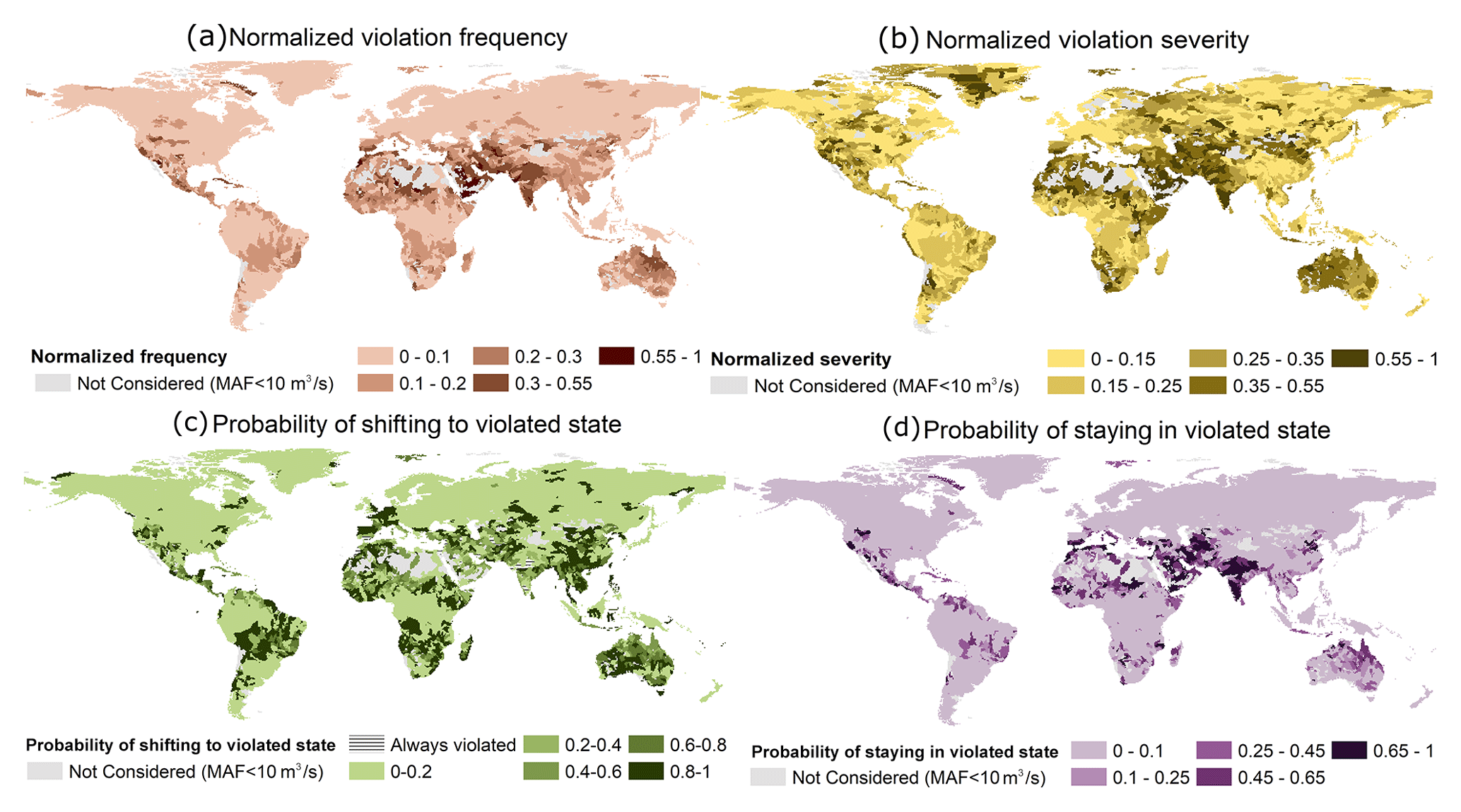
Figure 2 Four measures of environmental flow envelope (EFE) lower or upper bound violation estimated using the ensemble median of four global hydrological models: (a) normalized frequency of violation, (b) normalized severity of violation, (c) probability of shifting to a violated state from a non-violated state, and (d) probability of staying violated once shifted to a violated state.

Although the majority of regions with high P.shift values were arid or semi-arid, some exceptions included southeastern Asia and Central South America. The non-arid regions with higher P.shift values also have extremely high water withdrawal in all sectors (agriculture, domestic, and industry). This spatial concurrence suggests that human activities, as well as hydroclimatic influences, play a significant role in deciding a region's P.shift. However, once in the violated state, the flow variability regimes in the catchment determine the probability of remaining (P.stay) in the violated state. Catchments with highly variable flow regimes (i.e., that receive most of the annual flow as floods; see Fig. S2 in the Supplement for a classification map) have higher probabilities of staying violated once shifted, whereas catchments with stable flow regimes (year-round steady high baseflow) have a higher tendency to revert to a non-violated state. An example of this behavior can be seen in the Australian basins. Though almost all the Australian basins have a very high P.shift, only the highly variable flow regime northern catchments have a high probability of staying violated. Despite having an exceedingly high P.shift, the southern stable catchments swiftly shift back to a non-violated state.

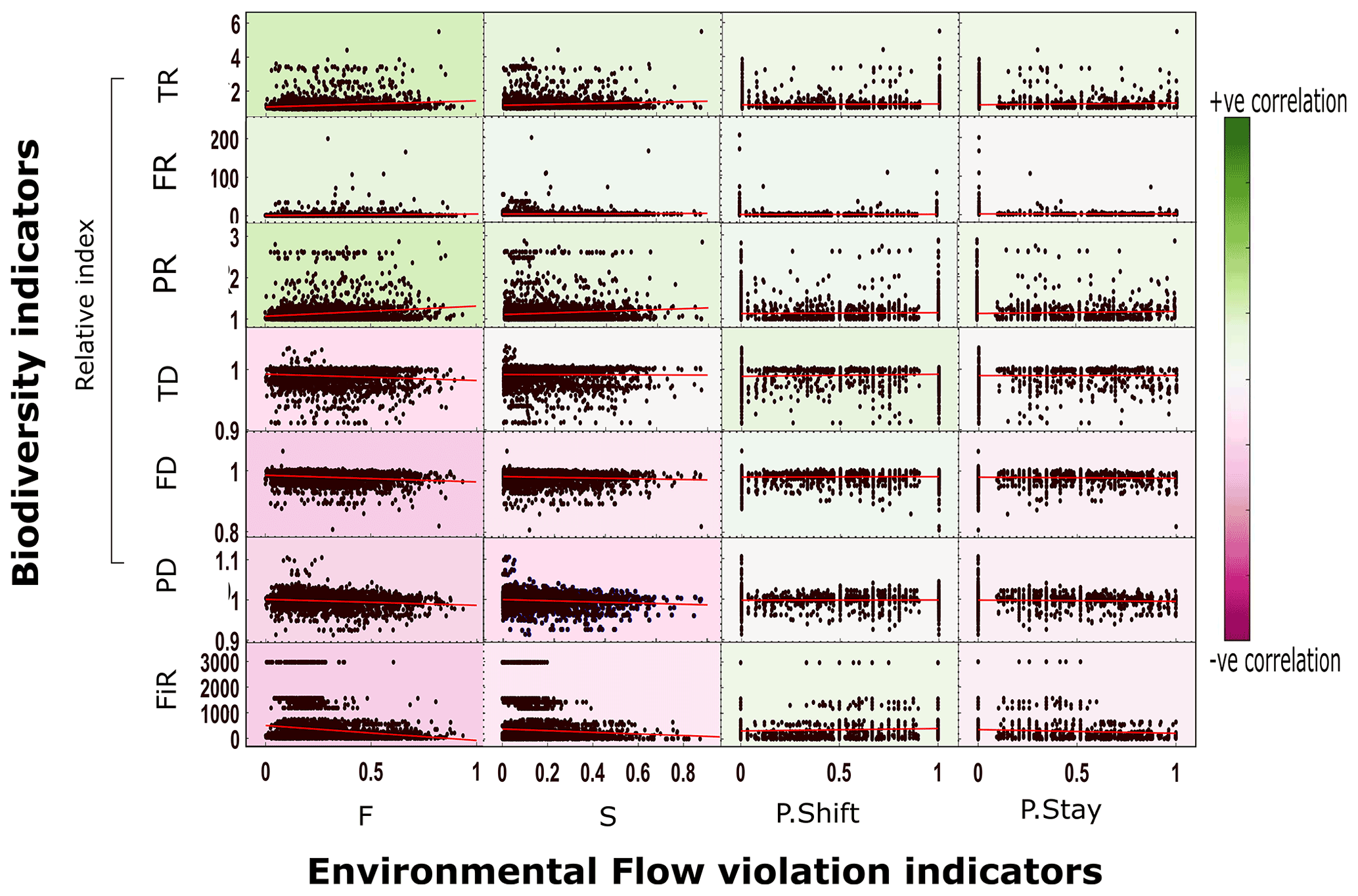
Figure 3 Scatter between EF violation indices and biodiversity indices (plots include linear fits) at a globally aggregated scale. Note: this figure represents results from case 1 (level 5 HydroBASIN matched with biodiversity data). The results of other aggregation methods are given in the Supplement (Figs. S5 and S6). Abbreviations: F – frequency of violation; S – severity of violation; P.shift – probability of shifting to a violated state; P.stay – probability of staying in a violated state; FiR – fish richness; TR – taxonomic richness; FR – functional richness; PR – phylogenetic richness; TD – taxonomic dissimilarity; FD – functional dissimilarity; PD – phylogenetic dissimilarity.

3.2 Relationship between EF violation and freshwater biodiversity

The aggregated analysis was carried out at global and ecoregion scales. Multiple aggregation methods (Sect. 2.3) yielded comparable results, so only case 1 (level 5 HydroBASIN matched with biodiversity data) results are discussed further (see Figs. S5 and S6 for results obtained using other aggregation methods). At the global scale, none of the biodiversity indicators correlated (significance of p value was < 0.05) with any EF violation indices (Fig. 3). The biodiversity indicators do not exhibit any strong trend in either the positive or the negative direction. The correlation coefficient value (R value) for the remaining biodiversity indicators only ranges from −0.2 to 0.17 (Fig. 3b). The three fish dissimilarity facets (TD, FD, and PD) show a slight negative correlation whereas the richness facets (TR, FR, and PR) display a slight positive correlation with EF violation. The positive correlation of the richness indicators is attributed to an overall increase in the assemblage in most of the basins despite the increase in EF violation. Moreover, (relative) TR and (absolute) FiR show opposite trends. The positive trend in TR could be attributed to changes involving nonnative species, whereas the FiR describes the current deteriorated state. The increase in the fish assemblage over time was verified using an independent dataset, RivFishTIME (see Figs. S8 and S9) (Comte et al., 2021). The increase in the fish richness facets primarily stems from the introduction of alien species into streams for commercial purposes (Su et al., 2021). The invasion of alien species can tamper with the existing natural ecosystem equilibrium, resulting in further degradation of the overall ecosystem health. The results obtained using RivFishTIME datasets were also consistent with the findings obtained using FiR and six relative biodiversity indicators, and there was no significant correlation between EF violation indicators and fish abundance data over time (see the results for five selected fish species based on data completeness and geographical distribution shown in Sect. S8; Fig. S8).

Correlations between EF and biodiversity are generally weak at the scale of G200 freshwater ecoregions as well (see Sect. 2.2, Olson and Dinerstein, 2002). In G200 freshwater ecoregions (see Table S6 for the full freshwater ecoregion results), the nature of the EF–biodiversity relationship greatly varied between different ecoregions (Fig. 4). In large lakes, large rivers, and small lakes the richness indicators obtained from Su et al. (2021) (TR, FR, PR) showed a strong and significant positive correlation with most of the EF violation indices. The increase in biodiversity despite an increase in EF violation could be a signal of the introduction of nonnative species for commercial purposes, whereas, in large rivers, large river deltas, and xeric basins, the dissimilarity indices and FiR show a negative correlation. However, in most ecoregions, the EF–biodiversity relationship is insignificant (p value > 0.05). Similar analysis using different aggregation/scale matching methods also yielded comparable results at the G200 ecoregion scale (see Figs. S5 and S6). In addition to this, the multivariate regression analysis results (Fig. 5) also show a very low correlation between EF violation indicators and biodiversity indices in most G200 ecoregions except small lakes, where the coefficient of determination is between 0.25–0.4 for the richness indicators (TR, FR, PR). The mean coefficient of determination (r²) is approximately 0.1. These results corroborate the above findings that EF violations are not significantly inversely correlated with biodiversity, regardless of the ecoregion, for the current dataset.

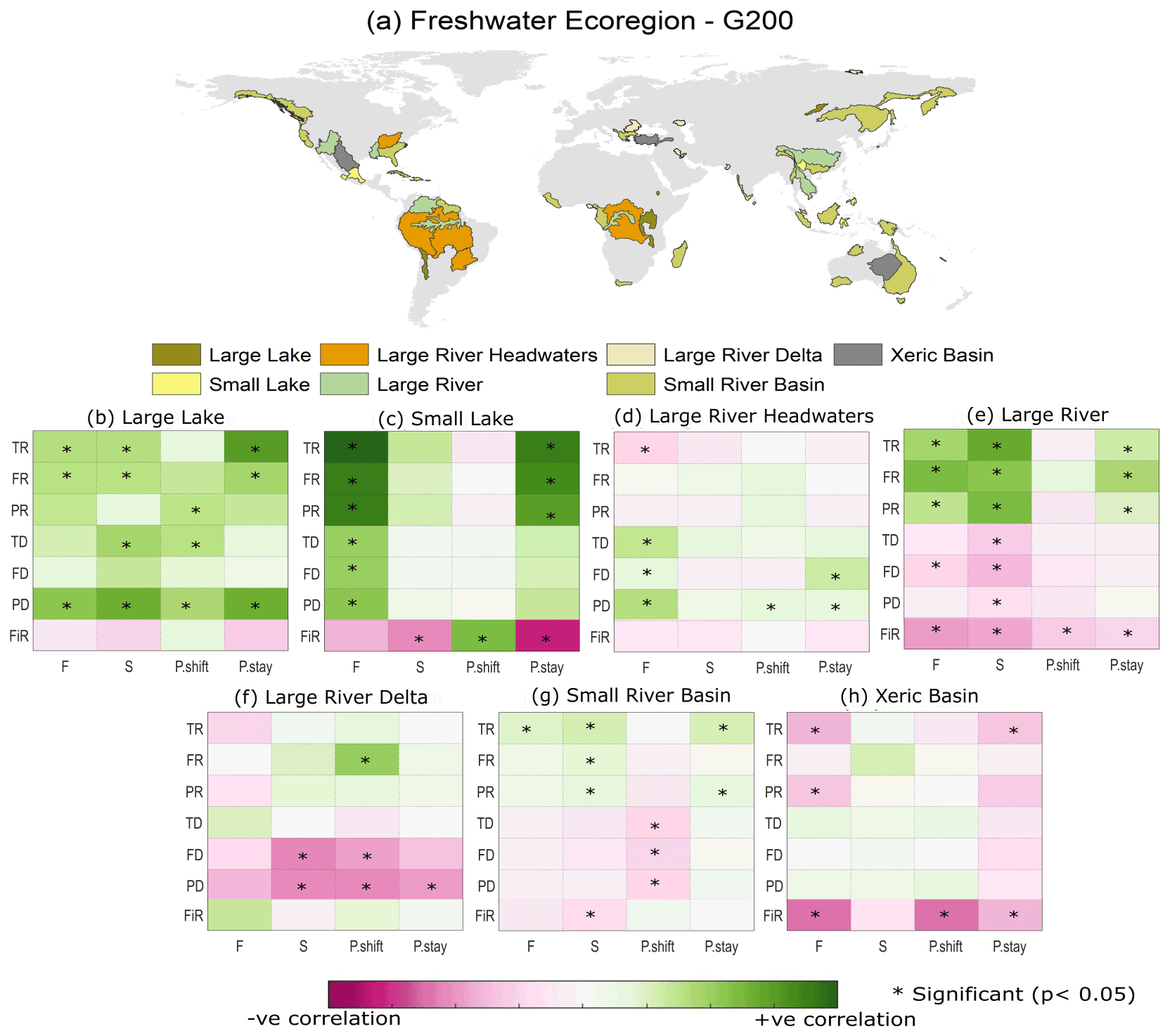
Figure 4 (a) Spatial distribution of different G200 freshwater ecoregions and (b–h) the correlation between EF violation indices and freshwater biodiversity indicators for different G200 freshwater ecoregions. Note: the results for all the WWF freshwater ecoregions are given in the Supplement (Sect. S7). Abbreviations: F – frequency of violation; S – severity of violation; P.shift – probability of shifting to a violated state; P.stay – probability of staying in a violated state; FiR – fish richness; TR – taxonomic richness; FR – functional richness; PR – phylogenetic richness; TD – taxonomic dissimilarity; FD – functional dissimilarity; PD – phylogenetic dissimilarity.

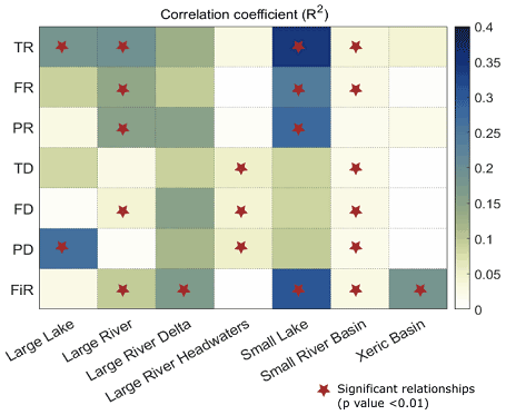
Figure 5 Coefficients of correlation (R²) for multivariate regression between EF violation indicators and biodiversity indices. Each row represents one biodiversity indicator and each column represents one G200 ecoregion.

4 Discussion

The findings from this study indicate that the EF–biodiversity relationship is poorly correlated at global or ecoregion scales with currently available data and methods. The most likely explanation for the lack of correlation is the overwhelming heterogeneity of the freshwater ecosystems – e.g., with some freshwater species being more susceptible to variations in flow than others (Poff and Zimmerman, 2010) – which is not adequately represented in the spatial resolution used (level 5 HydroBASIN). Moreover, when it comes to a larger-scale relationship, several other factors such as climate change (Davies, 2010; Poff et al., 2002), river fragmentation (Grill et al., 2015; Herrera-R et al., 2020), large-scale habitat degradation (Moyle and Leidy, 1992), landscaping/river scaping (Allan et al., 2005), alien species (Leprieur et al., 2008, 2009; Villéger et al., 2011), and water pollution (Brooks et al., 2016; Shesterin, 2010) can also impact the freshwater ecosystem in multiple ways. Thus, at the Earth system level, other interlinked factors potentially confound the impact of EF violation on biodiversity degradation.

4.1 Implications for water management

The lack of correlation between EF violation and freshwater biodiversity has implications for large-scale water management. A generalized large-scale EF approach can underestimate the stress on the ecosystem at a smaller scale where the actual action is taking place. It is undeniable that adequate flow is essential for maintaining freshwater ecosystems. Nonetheless, current generalized EF estimation methods need further refinement to adequately capture this importance. The global hydrological EF methods are often validated using locally calculated EF requirement values (Pastor et al., 2014) with the assumption of adequate scalability in the EF–biodiversity relationship. However, more holistic EF estimation methods combining hydrological, hydraulic, and habitat simulation methods and expert knowledge (Poff and Zimmerman, 2010; Shafroth et al., 2010) are essential to ensure a healthy freshwater biodiversity. The policies and decisions taken at various scales need a more dynamic framework where different dominant drivers of ecosystem degradation can be prioritized based on particular cases. For instance, an integrated EF indicator which encompasses quantity, quality, and timeliness of water in the streams will be a better hydrologic indicator to evaluate freshwater ecosystem health than an indicator which accounts only for quantity. Moreover, when making water management decisions, care must be given to account for the temporal and spatial heterogeneity in the ecosystem dynamics.

Although there are some coordinated scientific efforts such as ELOHA (Ecological Limits of Hydrologic Alterations) (Poff et al., 2010) to provide a holistic framework for EF estimation, its scientific complexity and high implementation cost constrains its use around the world (Richter et al., 2012). For example, several European countries such as Romania, Czech Republic, Serbia, and Luxembourg use a national-level static method to define minimum environmental flows (Linnansaari et al., 2012). Similarly, other jurisdictions use the presumptive standards proposed by Richter et al. (2012) to establish a legal basis for EF protection. These presumptive standards limit hydrologic modifications to a percentage range of natural or historic flow variability. One example of such a case, North Carolina's Environmental Flow Science Advisory Board, uses a presumptive standard of 80 %–90 % of the instantaneous modeled baseline flow as the EF requirement (NCEFSAB, 2013). The limitation of such a practice is the incorrect presumption of uniformity in the EF needs over a larger region. Therefore, we recommend the application of holistic indicators at these large scales (covering all river stretches and tributaries) rather than using simplified hydrologic-only metrics of EF (violation). However, the authors also acknowledge the limits in implementation of a more dynamic EF framework in data-limited regions. Programs for more monitoring and data collection and improved, more holistic modeling methods using more/better data need to be implemented in those regions. Thus, applying a holistic framework such as ELOHA could be made possible and can capture the heterogeneity in the EF–biodiversity relationship.

4.2 Implications for a water planetary boundary

The current rationale in using EF in the water planetary boundary relationship is based on the assumption of its universal relationship with freshwater biodiversity. However, with the currently available data and methods, the findings for the EF–biodiversity relationship are inconclusive. Moreover, due to the heterogeneity of biodiversity response over time and space, the trend at any aggregate scale is likely to remain relatively constant instead of showing any discernible tipping point (Brook et al., 2013). We suggest that the use of environmental flows in defining water planetary boundaries should be reconsidered, given the higher degree of heterogeneity and lack of strength of the ecosystem function–biodiversity relationship. Some of the potential reasons for this reconsideration are as follows. Firstly, freshwater biodiversity may not have pan-regional or “continental-planetary”-scale threshold dynamics, and its link with EF violation might be inadequate to represent the finer-scale variations. Secondly, resource distribution and human impact heterogeneity suggest the need for regional boundaries, as proposed by Steffen et al. (2015). Thirdly, the EF calculation methods used in the current regional/planetary boundary definition are highly restricted to hydrological methods, which may not be adequate to capture the biodiversity status. A regional boundary transgression can occur even well within planetary-level safe limits (Brook et al., 2013; Nykvist et al., 2017). Therefore, for an overly complex biophysical relationship such as EF–biodiversity, where multiple shift states are possible, it is difficult to prioritize and manage critical regions without a regional/local boundary.

4.3 Limitations and ways forward

1. Data scarcity: even though this study uses state of the art global hydrological models and best-available global estimates of EF requirements, freshwater ecological data are limited to freshwater fish. Several other taxa, such as crayfish and other benthic invertebrates, phytoplankton, or zooplankton, are also significant in determining the proper functioning of a freshwater ecosystem (AL-Budeiri, 2021; Domisch et al., 2017; Nyström et al., 1996). However, due to a lack of global data, these taxa are not included in this study. To better examine the relationship, global datasets for other freshwater biodiversity metrics are urgently needed.

2. Discrepancy in data resolution: the spatial and temporal resolutions at which the EF violation is estimated here and the biodiversity indicators measured/calculated are inconsistent. The basic spatial measuring unit of the biodiversity is sometimes greater or less than the basin size at which EF is measured. This discrepancy could have some impact on the results. However, in this study, several resolution-matching methods were used to account for this uncertainty. Therefore, more detailed data with better-matching scales are needed to overcome this limitation.

3. Lack of multi-driver interaction: in this study, we consider the impact of EF violations on biodiversity to be an independent relationship. In reality, this might not be the case. Other drivers of ecosystem degradation, such as land use change, habitat loss, stream modifications, and geographical disconnection can influence the EF–biodiversity relationship. These interactions were outside the scope of this study but should be taken into account in follow-up studies.

4. Simplified representation of human interference with freshwater systems: the role of humans in impairing the ecosystem balance is represented here based on how human water withdrawals violate the hydrologically defined EF. Other human disturbances are thus not accounted for, such as aquatic habitat degradation through a change in land use, artificial introduction of nonnative species, and non-point pollution from agriculture. Moreover, this study does not distinguish the climate-driven impact on EF violation from the anthropogenic impacts.

5. Exclusion of the impact of dams: the dams are indeed a large contributing factor to the uncertainty in the results. Dam-regulated rivers may have a significantly different effect on biodiversity compared to free-flowing rivers. The ISIMIP data used to calculate EF violations considers the effects of large dams on the streamflow. However, to explicitly isolate the effects of dams in this analysis from other drivers, information on dam operation schemes for each sub-basin would be necessary, and this would require a paper on its own. Therefore, the effects of the dams are incorporated in this study but are not explicitly analyzed separately from other drivers.

5 Summary and conclusion

The relationship between EF violations and freshwater biodiversity was evaluated at globally aggregated levels in this study. No significant relationship between EF violation and freshwater biodiversity indicators was found at the global or ecoregion scale using globally consistent methods and currently available data. Relationships may exist at smaller scales and could potentially be identified with more holistic EF methods that include multiple factors (e.g., temperature, water quality, intermittency, connectivity) and more extensive freshwater biodiversity data. A single negative result is not a final say, but it is a call to conduct more study on existing generalized and well-applied methods.

The paper is not intended to be a definitive test on the relationship between EF and aquatic biodiversity, but more to be an exploratory analysis that tests a widely used but rarely verified assumption of the relationship at the global and ecoregion scale. The lack of correlation in the EF–biodiversity relationship found in this study suggests that particular care should be taken when developing macro-scale EF policies (regional and above), and further implies that the conceptualization of a blue water planetary boundary ought to rest upon a broader set of relationships between hydrological processes and Earth system functioning. At larger scales, the enormous spatial and temporal heterogeneity in the EF–biodiversity relationship motivates a holistic estimation of EF grounded in ecosystem dynamics.