Technical Note: Space–time statistical quality control of extreme precipitation observations

Information about precipitation extremes is of vital importance for many hydrological planning and design purposes. However, due to various sources of error, some of the observed extremes may be inaccurate or false. The purpose of this investigation is to present quality control of observed extremes using space–time statistical methods. To cope with the highly skewed rainfall distribution, a Box–Cox transformation with a suitable parameter was used. The value at the location of a potential outlier is estimated using the surrounding stations and the calculated spatial variogram and compared to the suspicious observation. If the difference exceeds the threshold of the test, the value is flagged as a possible outlier. The same procedure is repeated for different temporal aggregations in order to avoid singularities caused by convection. Detected outliers are subsequently compared to the corresponding radar and discharge observations, and finally, implausible extremes are removed. The procedure is demonstrated using observations of sub-daily and daily temporal resolution in Germany.

1 Introduction

A clear definition of an outlier might be intuitive to many, but it has been formulated differently by several researchers. In the work of Barnett and Lewis (1994), an outlier was defined as an observation showing an inconsistent behavior compared to other data values. Hawkins (1980) described an outlier as being an observation that differs substantially from other observations, as if it might have been produced by an alternating mechanism. More precisely, for Iglewicz and Hoaglin (1993), an outlier is an observation that arouses suspicion to the analyst and does not belong to the same data distribution. In general, there are two types of outliers, namely those associated with an error and those associated with a real observation. The reasons for an observation being erroneous could be due to instrumental errors (e.g., use of false instrument, equipment malfunction, and false equipment operation) and/or human errors (false reading or recording or even computation of observations). Moreover, errors can occur if the measuring site is falsely chosen, thus providing a false representativeness of the observed process.

Hydroclimatological data are of a unique nature as they occur in a non-repetitive manner. If an observation is not registered correctly, reconstructing it is very challenging, especially for precipitation values. However, reliable information about precipitation extremes is essential for many design purposes such as flood analysis, extreme value statistics, and stationarity analysis, to name just a few.

Many quality control (QC) algorithms have been developed and are being used by weather service agencies to minimize and detect false measurements. Durre et al. (2010) established a comprehensive QC algorithm for daily surface meteorological observations (temperature, precipitation, snowfall, and snow depth). For precipitation data, the QC method for detecting false observations consisted of several steps. A climatological outlier check is used for flagging values exceeding a certain temperature-dependent threshold and a spatial consistency check based on comparing the target observation to neighboring ones. An observation is eventually flagged if the difference exceeds a certain climatological percent rank threshold. Qi et al. (2016) implemented a QC algorithm to identify erroneous hourly rain gauge observations by using additional information as radar quantitative precipitation estimates (QPEs). A common practice for detecting outliers is to use an interpolation method to estimate the probability of a local observation using the surrounding locations. If this probability is very low, then the observation is suspicious. This was mathematically formulated by Ingleby and Lorenc (1993). In the work done by Hubbard et al. (2005), a QC method was developed for daily temperature and precipitation values consisting of four steps. Observations are flagged if they do not fall within ±3 SD (standard deviation) of the long-term mean and if they differ from the estimated value using a spatial regression technique. Some other QC methods are available but are often limited to time series analysis and tend to disregard the spatiotemporal extent of precipitation.

Precipitation observations have a space–time dimension. Observations are taken at different locations in space and in discrete time intervals. Due to the presence of non-negative and many no-precipitation (zero) values, precipitation data (especially at daily and sub-daily resolution) have a positively non-normal skewed distribution with heavy tails (Klemeš, 2000) and fall under the zero-inflated data. Therefore, an adequate transformation of the data should be performed to reduce the effect of the data skewness. A relatively simple approach to normalizing a variable is the Box–Cox transformation (Box and Cox, 1964).

The following work proposes a statistical space–time methodology based on interpolation in a cross-validation mode to find possible outliers in precipitation observations across several temporal aggregations. An outlier is defined here as an observation that strongly differs, for a certain temporal aggregation, from its spatial neighboring locations. A difficult task while working with outliers in general, and especially in hydrology, is distinguishing between correct and false observations. Therefore, to validate the detected outliers, the suspected values are additionally compared to independent information such as discharge and radar measurements.

This paper is organized as follows: after the introduction, the data and methodology are presented. Afterward, the results of the outlier detection are presented, and four examples of verification via subsequent comparison to radar or discharge data are shown. In the final section of the results, the number of identified outliers for every year (and month) and for each location is mapped and presented.

2 Study area and data

This study was done using the Germany-wide precipitation data set from the German Weather Service (DWD), which covers an area of approximately 357 000 km². The average annual rainfall in Germany is around 800 mm and can reach up to 2100 mm in the higher elevations of the Alps in the south. Currently, the DWD operates a network of rain gauges with different temporal resolutions ranging from every minute to every day. Hourly and sub-hourly data are available from the 1990s onwards. The number of these stations has been continuously increasing since then. On the other hand, the number of stations with daily observations has also started to decrease since then as they have been replaced by automatic rain gauges. Rain gauges near the border (30 km inland buffer) were not included in this analysis.

In the 1990s, most DWD rain gauges were tipping buckets or drop counters. From 2000 onwards, these were replaced by weighing gauges (OTT Pluvio), and since 2017 these have been replaced by combined tipping bucket and weighing rain gauges (LAMBRECHT meteo GmbH rain[e] model).

Precipitation data from the recent DWD observation network go through several quality control steps. The first step is a quality control directly at the automatic stations. Since this is an automatic test, relatively wide thresholds are applied. It includes tests for completeness, thresholds, and temporal and internal consistency. Based on these tests, a quality flag is assigned to the data. The data are then submitted to a database. Another test with tighter thresholds is then performed based on the QualiMET software (Spengler, 2002). This phase of the quality check also tests for completeness and climatological, temporal, spatial, and internal consistency. Questionable values are manually checked and corrected, and the quality label is adjusted. A final quality check step occurs after all of a month's data are available, by focusing on aggregate values. The quality flags are stored in the database and are also made available to users. DWD quality assurance also includes the identification and correction or description of errors in the historical data (Kaspar et al., 2013). Appropriate procedures have been developed for the quality control of historical data. In general, the quality of these values can be considered reasonably good, but there are still doubtful values of the order of about 0.1 %–1 %, especially for the pre-1979 data. The user must keep in mind that the data can be affected by certain non-climatic effects, such as changes in instrumentation or observation time. With few exceptions, the data are reported “as observed”, i.e., no homogenization procedure was applied.

As independent data for verification, radar-derived rainfall QPE and discharge observations from the state of Bavaria were used. The radar data used are from the product RADOLAN-RW that is provided by the DWD in hourly and daily resolutions starting in the year 2005 (DWD Climate Data Center, CDC, 2021a). These products have been gauge-adjusted with the observed hourly station data. The occurrence (or absence) of precipitation observation in the radar data over the target location is an indication of the quality of the observation. The discharge data were quality checked and provided by the environmental agency of Bavaria with hourly and daily resolutions for approximately 400 gauges within the region of Bavaria (Bayerisches Landesamt für Umwelt, 2022). Different headwater catchments were derived and selected for the validation of the results. A reaction (within few hours) in the headwater catchment discharge is expected after the event occurred in case of correct rainfall observations.

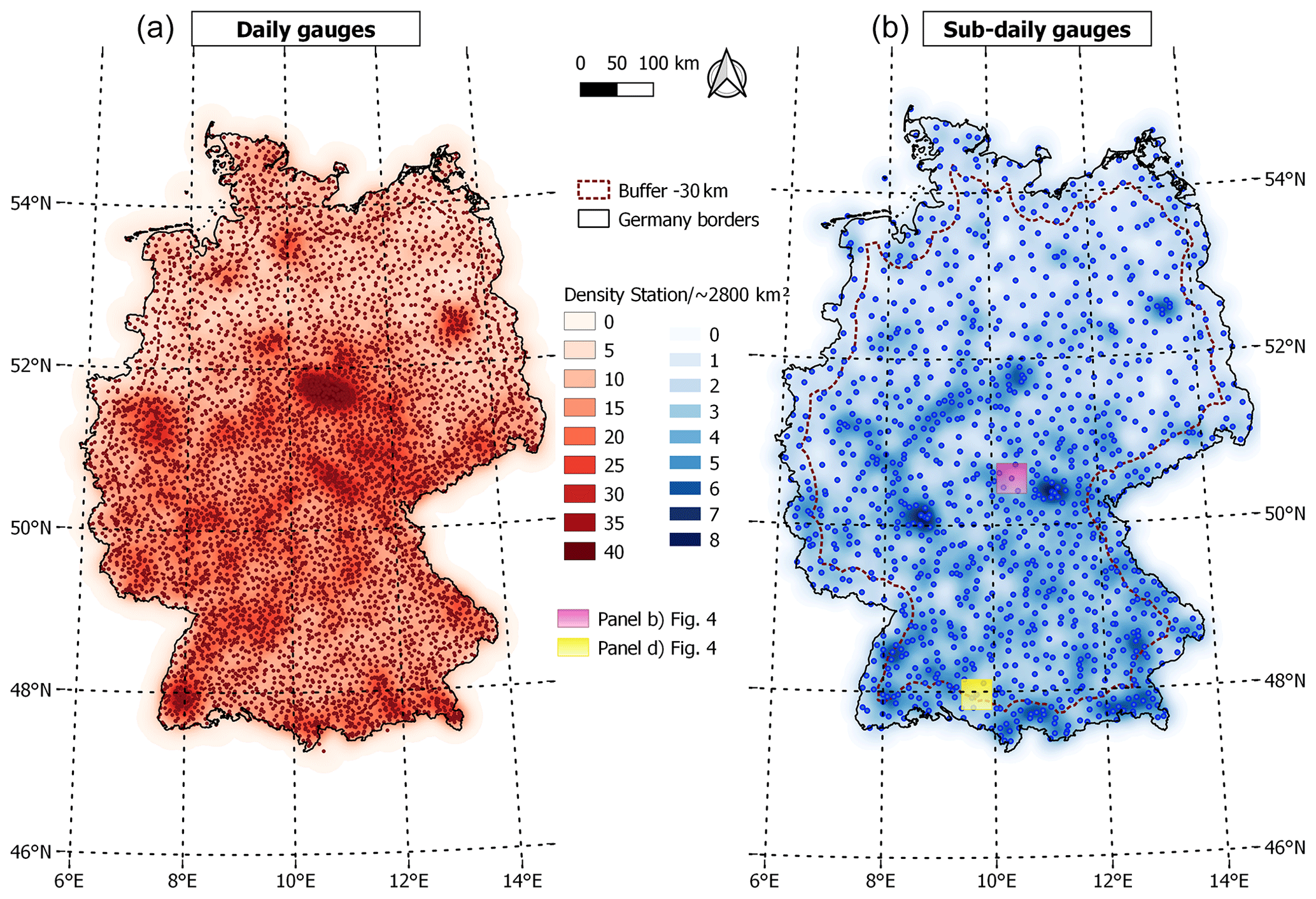
Figure 1 Map of the study area showing the location and density (number of stations per ∼2800 km²) of the DWD gauges with daily (a) and sub-daily (b) resolutions. The yellow and pink boxes in the map on the right refer to the two locations of the examples presented in Fig. 4.

Figure 1 illustrates the location of the daily and sub-daily rain gauges and their spatial density. For the daily data, all available locations (historical and present) are displayed. The stations do not have a homogeneous spatial distribution over the study area, where some locations have a higher network density than others. The spatial density was calculated using a kernel density estimation (KDE) with a quartic shape and a radius of influence of 30 km. The estimated density value depends on the separating distance between the known and unknown locations and the kernel parameters. This is the bandwidth (h) which is reflected by the radius of influence and the weighting function or kernel function K. The latter defines the contribution of each point as a function of the separating distance. Further detail regarding KDE estimation can be found in Yu et al. (2015).

3 Methodology

3.1 Data transformation

As an initial step, a Box–Cox transformation, as described by Eq. (1), was applied for every variable X and temporal aggregation t to reduce the effect of the skewed precipitation distribution (Box and Cox, 1964).

$$\begin{array}{}\text{(1)}& X_t^{*}=\left\{\begin{array}{lc}\frac{\left(X_t^{\mathit{\lambda }}-\mathrm{1}\right)}{\mathit{\lambda }}& \mathrm{if}\mathit{\lambda }\ne \mathrm{0}\\ \log \left(X_t\right)& \mathrm{if}\mathit{\lambda }=\mathrm{0}\end{array}\right.,\end{array}$$

where X^* is the transformed precipitation data at location u and temporal aggregation t. X is the original precipitation data at location u and temporal aggregation t. λ is the transformation factor for temporal aggregation t.

To find which transformation factor λ is most suitable, several simulated lower truncated standard normal distribution functions (sampling space bounded by [$-\mathrm{\infty }<a=p_{\mathrm{0}}$, $b=+\mathrm{\infty }$]) were fitted to the original data (Burkardt, 2014). The probability of having a value above or below p₀ is then derived (p₀ probability of having 0 mm precipitation value).

From this probability (denoted p_norm), a new standard normal distribution is generated, where ($x<p_{\mathrm{norm}}=\mathrm{0}$, x>=p_norm=x). From this distribution, the skewness γ_norm is calculated. The goal now is to find which transformation factor minimizes the difference between the original data skewness and γ_norm. This was done for each station separately and for all aggregations. Eventually, an average transformation factor (denoted hereafter λ) was derived for each temporal aggregation. The results of this procedure can be seen in Table 1.

Table 1 Average transformation factor λ used to transform the original data to the truncated normal space with reduced skewness.

Once λ was calculated, the original precipitation data were transformed, as in Eq. (1), and in the newly truncated normalized space, the following approach was implemented to find outliers in the precipitation data over several temporal resolutions.

3.2 Outlier detection

The proposed method was initially tested for identifying outliers in groundwater quality data (Bárdossy and Kundzewicz, 1990). In this paper, a similar method was implemented to identify unusual precipitation data and was extended by a validation of the results using external information, such as radar or discharge observations. For detecting possible outliers, the concept of jackknifing is used, a method initially developed by Quenouille (1949, 1956). The main idea is based on removing one (or each) observation from the data and estimating its value again. In this study, the four largest annual observations for every station are compared to the estimated values at the same location. Each cross-validated value is estimated using the nearest 30 neighboring locations with valid observations. This is needed for a reliable estimation of the variogram and has less influence on the estimated value due to the shading effect in kriging, i.e., the stations further away have smaller weights.

Since many possible faulty observations can only be detected at a lower temporal resolution, the procedure was applied over several temporal aggregations. For example, when looking at sub-daily and sub-hourly values, a single observation might not be unusual, but the accumulation of many values reveals suspicious sums. Furthermore, single events might occur at high temporal scales (e.g., hourly) and are not detected at lower aggregations (e.g., daily).

For estimating the target value, ordinary kriging (OK) is used as an interpolation technique. It is a regionalization method, initially introduced by Krige (1951) and Matheron (1962), to estimate an unknown value at a target location by solving a linear equation system by minimizing the estimation variance and maximizing the accuracy (no systematic error). The spatial correlation structure is reflected by the variogram which is derived in the rank space domain and rescaled to the variance of the data. This allows for variogram calculation in a more robust manner (Lebrenz and Bárdossy, 2019). The target location is calculated by solving the kriging equation, and the estimation variance is noted. For identifying unusual observations, the ratio between the absolute value of the difference between the observed and the estimated values and the estimation variance is calculated. This criteria ratio (CR) describes the relative agreement/disagreement between the observed value and the spatial surroundings for the corresponding time step. Larger CR values reflect high spatiotemporal disagreement, and low values denote greater agreement. Based on the CR value, different types of events can be identified, namely those occurring on a local scale, with high CR values, and others on a regional scale, with low CR values. Following Bárdossy and Kundzewicz (1990), a CR value of 3 is initially used to identify suspicious observations. The CR value is derived for every cross-validated event. Eventually, the CR value is related to all of the observed (interpolated) data, establishing a possibility of finding a suitable CR value for identification of precipitation outliers.

$$\begin{array}{}\text{(2)}& {\mathrm{CR}}_i\left(u\right)={\displaystyle \frac{\left|Z_i^{*}\right(u)-Z_i(u\left)\right|}{{\mathit{\sigma }}_i\left(u\right)}},\end{array}$$

where $Z_i^{*}\left(u\right)$ is the estimated value at location u and time step i. Z_i(u) is the observed value at location u and time step i. σ_i is the kriging standard deviation at location u and time step i.

Since precipitation events occurring on a local scale might represent an actual small-scale event and not a false value, to validate the first or the second case, the suspicious events are compared to the observed radar QPE or discharge values in the corresponding catchment. Despite having their own drawbacks, the radar and discharge observations are used here as a qualitative decision support tool.

The flowchart in Fig. 2 describes the implemented space–time precipitation outlier detection scheme.

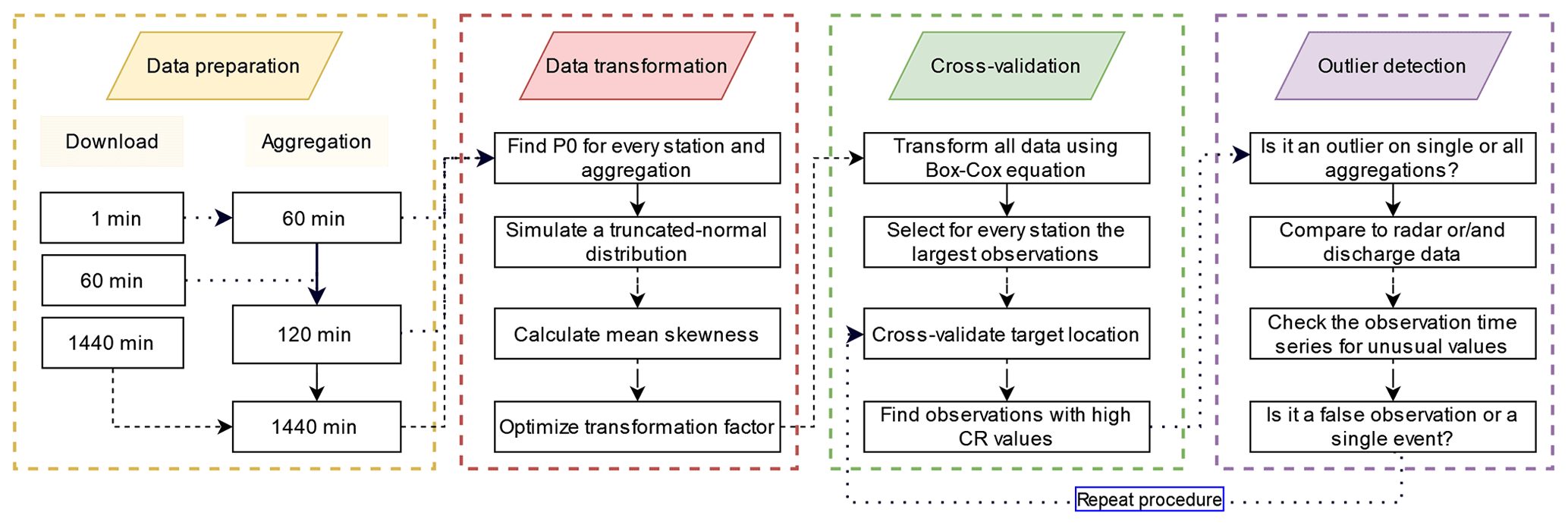
Figure 2 Flowchart summarizing the described method, starting with the data download procedure and ending with the identification of suspicious observations.

3.3 Data corruption

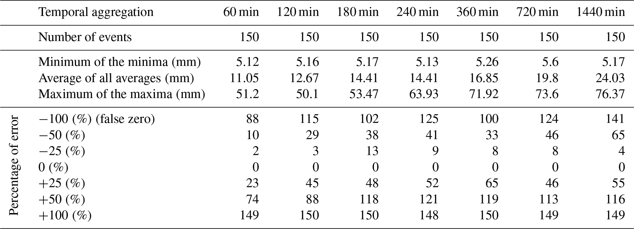
To further test the validity of the method, 20 stations without any detected outliers were randomly selected and their data (same events as before) were artificially manipulated, such that the transformed observations of each target location were decreased and increased by several percentages (from 25 % to 100 %), and the outlier detection method was tested. The results of this procedure can be seen in Table 2. By decreasing the observed value until a false zero observation was reached, the method was able to identify, on the hourly scale, around 60 % and, on the daily scale, 94 % of the cases as being outliers. On the other hand, by increasing the error value to up to 100 %, almost all values were detected on all temporal aggregations. This emphasizes the validity of the method, especially regarding identifying false high observations.

Table 2 Number of newly detected events after corrupting, by different percentages, the cross-validated observations of 20 randomly selected stations with no previous outliers.

4 Results

4.1 Outliers vs. single events

The center panel of Fig. 3 represents the CR value versus the ratio between the interpolated and observed values. All values denoted in red have a CR value above 3. This figure allows the identification of the events that are of interest and relates the CR value to the interpolated and observed data. Note that the observed and interpolated values are in the original non-transformed space; only the CR values are calculated from the interpolation of the transformed values.

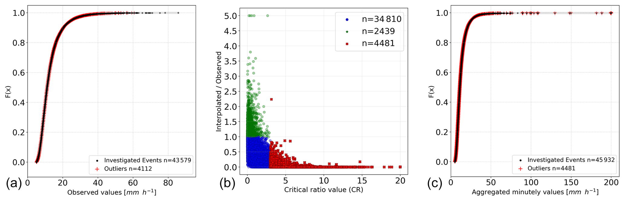
Figure 3 Panel (a) shows the CDF of all investigated hourly events, with the detected outliers marked in red. Panel (b) shows, for the data aggregated at every minute, the CR values versus the ratio of interpolated and observed hourly values. Panel (c) shows the CDF of all investigated hourly events, with the detected outliers marked in red. The hourly data in the center and right panels were aggregated from the minute values. Note that an upper limit of 200 mm h⁻¹ was set.

The values in the plot, with a ratio of interpolated to observed of 5, are values obtained when a neighboring station (or stations) had simultaneously recorded an outlier (in this case a false high observation). This leads to detecting a false outlier. This can be accounted for by running the method again after all neighbors have been checked.

In the left and right panels of Fig. 3, the cumulative distribution function (CDF) from all investigated observations was calculated, and the location of the detected outliers is marked. The events that were detected as being outliers were spread over the curve, showing that the method can detect not only high values but also relatively small values that differ highly from their neighboring space.

The left panel in Fig. 3 shows the results for the original hourly observations. The right panel shows those for the aggregated observations for every minute. By comparing the two, the quality control procedure of the DWD can be investigated. Spatial consistency is checked more intensively by the DWD for higher aggregated precipitation data (≥1 h) than for high temporal resolution data (e.g., 1 min). For example, in the hourly data, none of the largest sums (>60 mm h) is detected as being an outlier, and only one observation is larger than >80 mm h. In the hourly data based on the data aggregated for every minute, many values above 80 mm h exist and are mostly all detected as being suspicious. There are even unrealistic values with accumulated sums above 200 mm h which can be caused by several faulty small measurements or a few single large spikes in the data.

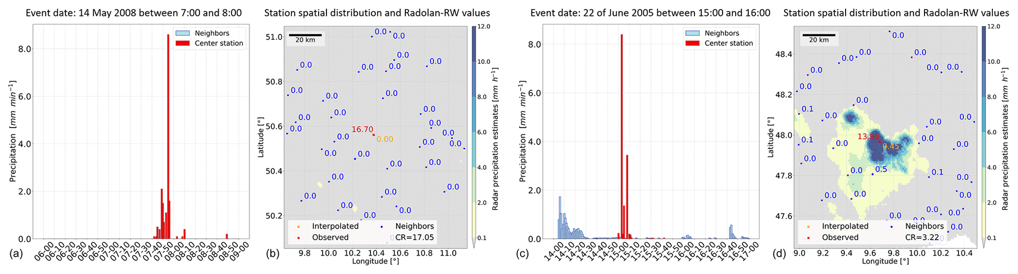
Figure 4 Two examples are shown, i.e., (a) an identified false observation and (c) a plausible event. Panels (b) and (d) show the values at the neighboring stations (in blue), the observed value (in red), the estimated value (in orange), and the RADOLAN-RW QPE data for that hour.

4.2 Selected case studies

The first example in Fig. 4a shows the presence of unusual values in the data for every minute of the cross-validated station (>8 mm min⁻¹). The radar data for that hour do not show such a high-intensity event above the investigated location. The second example, in Fig. 4c, shows a similar case in the data for every minute, but the radar image confirms the occurrence of the event.

Discharge data from small headwater catchments in the federal state of Bavaria with one (or many) rain gauge stations within the catchment were analyzed. If a rain gauge observation was identified as being suspicious, then the discharge values for the next hours following the event were checked. An example of this is shown in the upper Pegnitz catchment, which is located in northern Bavaria (Fig. 5). Figure 5b shows an hourly outlier observation that resulted in a reaction in the corresponding headwater catchment. On the other hand, Fig. 5c shows the opposite case, i.e., an hourly outlier that did not cause any reaction in the Pegnitz catchment.

Figure 5 Location of the discharge and rain gauge station within the Pegnitz headwater catchment (a). Observed discharge and precipitation data (±1 d) for detected outliers with (b) a discharge increment and (c) without a discharge increase.

4.3 Results over all stations and aggregations

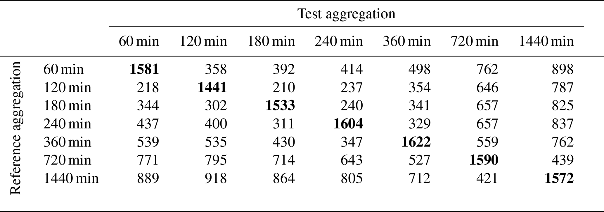
The method was applied over several temporal aggregations (hourly to daily), and events that are suspicious over single or several aggregations were identified. The result of this can be seen in Table 3. The diagonals show events that are common over the corresponding test and reference temporal aggregation. Some observations are only suspicious until a temporal aggregation is reached or exceeded, beyond which they are not detected anymore. The result of this can be seen in the values above and below the diagonals in Table 3.

Table 3 The diagonals show the total number of detected outliers per aggregation. The values above the diagonals reflect the number of different days between the reference and test aggregation. For example, there are 358 d in the reference 60 min aggregation that are not in the test with the 120 min aggregation.

The number of active stations (and device quality) affects the number of detected outliers. The red curve in Fig. A1 represents the ratio of detected outliers to the number of active stations (for every hour), which is shown by the blue curve. As the number of active stations increases, the number of detected outliers decreases, which is an indication that the quality of the observations is improving with time. In Fig. A1a, the effect of seasonality was inspected. The detected outliers were grouped by the month in which they occurred. The results show that, in the summer period, the number of detected outliers is much larger than in the winter period. This is related to convectional rainfall processes occurring in the summer period, leading to more small-scale single events. Finally, the percentage of outliers in the investigated events of every station for the hourly aggregated data is presented in Fig. 6. The map does not present any clear structure related to elevation and topography. Moreover, the map shows that outliers can happen everywhere, meaning that this is not a systematic problem.

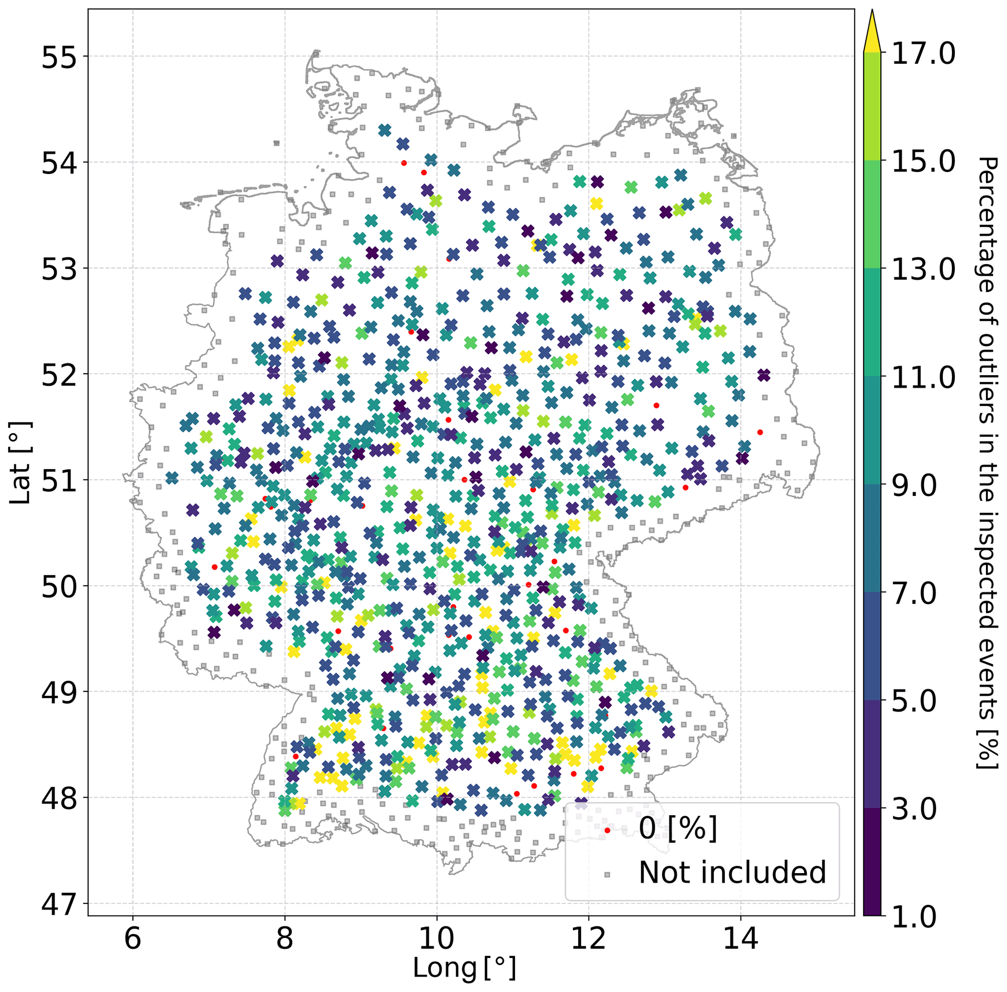
Figure 6 The figure shows the percentage of outliers in the investigated events of every station.

5 Conclusion

In this study, a methodology to identify outliers in precipitation data was presented. Due to the high spatiotemporal variability in precipitation, the quality control of precipitation data takes on a special task among meteorological parameters. Therefore, a transfer of the procedures developed in this paper to other variables is not necessarily reasonable. From an hourly to a daily temporal aggregation, the four largest yearly values for every station were inspected. To cope with the skewed rainfall distribution, a Box–Cox transformation with a suitable parameter was applied. The results revealed different outliers throughout various temporal aggregations. To test the robustness of the method, data from stations with no outliers were corrupted with several percentages and checked again. The method was able to identify most events as outliers, as the value of the added error increased. Seasonality was seen to play a major role in the number of detected outliers, and as the quality of the observations improved, the number of detected outliers (namely the false measurements) decreased. To distinguish between a false observation and a single event, external data were used. Discharge gauge data of corresponding headwater catchments and radar rainfall images were used when available. A final choice regarding flagging an observation is done carefully and individually for every location. Eventually, the flagged observations are kept aside and investigated before being used in further analysis.

The current method needs to be extended and modified for temporal aggregations below the hourly scale. In particular, the kriging methodology should include time as a third dimension to account for advection and correlation between subsequent steps. Moreover, many events are identified as being an outlier when part of the neighboring stations had zero precipitation values. This can happen in the case of directional-dependent events driven by a frontal system. These cases could be further handled by including anisotropy in the interpolation method.

Appendix A

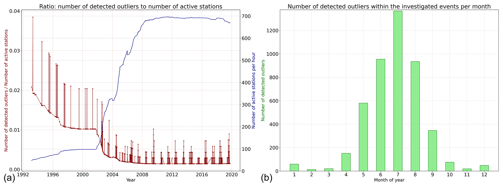
Figure A1 Panel (a) shows the number of hours with outliers within the investigated hourly events (aggregated from 1 min) of all stations per year. Panel (b) shows the number of detected outliers within the investigated events for every month within the hourly data using a CR value of 3.