Towards a hydrogeomorphological understanding of proglacial catchments: an assessment of groundwater storage and release in an Alpine catchment

Proglacial margins form when glaciers retreat and create zones with distinctive ecological, geomorphological and hydrological properties in Alpine environments. There is extensive literature on the geomorphology and sediment transport in such areas as well as on glacial hydrology, but there is much less research into the specific hydrological behavior of the landforms that develop after glacier retreat in and close to proglacial margins. Recent reviews have highlighted the presence of groundwater stores even in such rapidly draining environments. Here, we describe the hydrological functioning of different superficial landforms within and around the proglacial margin of the Otemma glacier, a temperate Alpine glacier in the Swiss Alps; we characterize the timing and amount of the transmission of different water sources (rain, snowmelt, ice melt) to the landforms and between them, and we compare the relationship between these processes and the catchment-scale discharge. The latter is based upon a recession-analysis-based framework. In quantifying the relative groundwater storage volumes of different superficial landforms, we show that steep zones only store water on the timescale of days, while flatter areas maintain baseflow on the order of several weeks. These landforms themselves fail to explain the catchment-scale recession patterns; our results point towards the presence of an unidentified storage compartment on the order of 40 mm, which releases water during the cold months. We suggest attributing this missing storage to deeper bedrock flowpaths. Finally, the key insights gained here into the interplay of different landforms as well as the proposed analysis framework are readily transferable to other similar proglacial margins and should contribute to a better understanding of the future hydrogeological behavior of such catchments.

1 Introduction

Glaciated catchments are highly dynamic systems characterized by complex physical, chemical and biological interactions at multiple scales ranging from local processes in the glacier ice to regional effects transmitted from the glacier forefield to downstream regions (Miller and Lane, 2018; Carrivick and Heckmann, 2017). In such environments, where nutrients and energy are limited and climate variations are large, glaciers provide water (Huss et al., 2017), sediments (Hallet et al., 1996) and organic carbon (Brighenti et al., 2019) to downstream areas, which sustain a high regional biodiversity (Milner et al., 2009). At the regional scale, glaciers provide a number of ecological services essential for human society, such as water supply for drinking water purposes and irrigation, hydropower or cultural services (Beniston et al., 2018; Haeberli and Weingartner, 2020). Water resource availability is undergoing strong seasonal modifications due to climate warming, with rapid glacier retreat worldwide (Milner et al., 2017), e.g., an estimated volume loss of 84±15 % by 2100 in the European Alps (Huss et al., 2017). Peak annual runoff from glacier melt will be reached between 2010 and 2060 across the world (Huss and Hock, 2018), and the subsequent reduction of ice available to melt, together with more liquid precipitation and earlier snowmelt (Lane and Nienow, 2019; Klein et al., 2016), will cause a change in streamflow regimes, with a shift in the flow magnitude and in the timing of high flows to earlier months (Berghuijs et al., 2014; Beniston et al., 2018; Gabbi et al., 2012; Lane and Nienow, 2019).

While numerous discussions of the implications of cryosphere changes have been published (e.g., Beniston et al., 2018; Huss et al., 2017; Immerzeel et al., 2020), the role of groundwater is typically neglected in many glaciohydrological studies in Alpine environments (Vuille et al., 2018). This is surprising given the rapidly growing body of literature on groundwater–snowmelt interactions, e.g., for environments with regular droughts (Fayad et al., 2017; Jefferson et al., 2008; Van Tiel et al., 2021), as well as regional studies highlighting large groundwater contributions to streamflows in the Andes (Vuille et al., 2018) and in the Himalayas (Andermann et al., 2012; Yao et al., 2021). Recent studies started to tackle this issue by estimating groundwater contribution at the catchment scale or by analyzing the hydrological processes of specific landscape units. At the catchment scale, water-stable isotopes as well as other geochemical tracers were used to identify groundwater contributions of 20 % to 50 % for sub-catchments with 25 % to 4 % glaciated cover (Penna et al., 2017; Engel et al., 2016, 2019). While those studies provide interesting insights into the role of groundwater to sustain baseflow, the allocation of storage to specific hydrological units remains unclear. This is problematic as such systems are subject to rapid geomorphological changes, with large areas of previously ice-covered till and bedrock becoming exposed in proglacial margins (Heckmann and Morche, 2019), leading to the emergence of new landforms that have high groundwater storage potential (Hayashi, 2020). Thus, studies focusing on the integrated catchment-scale response provide little information on the internal mechanisms which maintain baseflow, and they therefore cannot predict future changes in groundwater storage and its contribution to streamflow.

Figure 1 General overview of geomorphological landforms typical of proglacial zones. (1) Lateral moraine (grey); (2) debris cone; (3) talus slope (light grey); (4) fluvial outwash plain; (5) glacial deposit (till); (6) proglacial lake; (7) apparent bedrock (dark grey); (8) debris-covered rock glacier; (9) vegetation patches. Snow on the mountain tops is in white, and the glacier is in blue on the right (figure inspired by Temme, 2019).

Other studies have approached this issue by characterizing the structure and hydrological response of specific geomorphological units in terms of water partitioning, storage and release (Wagener et al., 2007). Those unconsolidated superficial landforms are formed by different glacial and slope processes, have different internal structures and sedimentology and create a complex mosaic of landforms in glaciated catchments, which we summarize in Fig. 1.

A recent comprehensive study of the hydrogeological processes in such geomorphological landforms was provided in the work of Hayashi (2020). Here, we only retain some key information. Morainic material can be deposited both on slopes or in flatter areas. They are composed of a non-sorted mix of fine to coarse materials, which may contain more consolidated till (Ballantyne, 2002). Where they are in contact with a stream network, complex interactions occur and relatively deep aquifers (10 m depth) can be formed, which may sustain baseflow during dry periods (Magnusson et al., 2014; Kobierska et al., 2015b). Heavily debris-covered relict glaciers lead to the formation of rock glaciers. They were shown to consist mainly of a coarse layer with high hydraulic conductivity but contain a 1 to 2 m basal layer of finer water-saturated sediments, which can store significant water amounts (Harrington et al., 2018; Winkler et al., 2016; Wagner et al., 2021). In flat valley bottoms, fluvial deposition of sandy–gravelly material will lead to the creation of so-called glaciofluvial outwash plains (Maizels, 2002). They collect water from multiple sources and maintain groundwater-fed river channels in fall, promoting habitat heterogeneity and high local biodiversity (Ward et al., 1999; Malard et al., 1999; Crossman et al., 2011; Hauer et al., 2016). Older outwash plains were shown to have strong interactions with glacier-fed streams (Ó Dochartaigh et al., 2019; Mackay et al., 2020) and to provide upward groundwater exfiltration contributing between 35 % and 50 % to river baseflow (Käser and Hunkeler, 2016; Schilling et al., 2021). On hillslopes, debris not linked to glaciogenic origin comes from rock slope failures, leading to the formation of talus slopes. These talus slopes are composed of coarser debris than morainic material, showing thereby little water retention capacity and fast water transfer to downstream units (Muir et al., 2011).

Those studies provide key information on the groundwater dynamics of selected units; they are, however, rarely integrated into a perceptual model that brings together knowledge of all units, which compares their relative storage volumes and their contribution to streamflow and thereby explains the overall catchment-scale hydrological response. To our knowledge, only a limited number of studies propose an integrated description of the hydrogeological behavior of proglacial margins: in the Canadian Rockies a series of papers studied the hydrogeology of different proglacial structures and were summarized in the work of Hayashi (2020); in the Cordillera Blanca in Peru a suite of studies (Baraer et al., 2015; Gordon et al., 2015; Somers et al., 2016; Glas et al., 2018) focused on the role of groundwater for streamflow in different proglacial valleys, and in the Swiss Alps, there is a review of the hydrological behavior of proglacial landforms by Parriaux and Nicoud (1990).

From our perspective, but as also highlighted by others (Heckmann et al., 2016; Vincent et al., 2019), there is still a need for integrative studies that (i) document the hydrological functioning of proglacial landforms with appropriate metrics, (ii) propose a framework to characterize the timing, amount and location of the transmission of different water sources (rain, snow, ice) to these landforms and between each of them, (iii) compare whether the documented response of individual landforms can explain the observed catchment-scale behavior in terms of streamflow amounts, timing and geochemistry and (iv) propose a unifying theory for the geomorphological, ecological and hydrological evolution of such rapidly evolving catchments.

Within this paper, we propose a framework to address the first three of the above-mentioned points. First, we present field observations from the Otemma catchment and our case study in the Swiss Alps (Sect. 2.1) and discuss the different hydrological behaviors observed around the outwash plain, based on electrical conductivity data, direction of groundwater flowpaths and an estimation of hydraulic conductivity (Sect. 3.1). We then propose a methodology to characterize the hydrological behavior of the different superficial landform storages by assessing their storage–discharge relationship based on recession analysis and a literature review of the timescales of their hydrological response (Sect. 3.3). Applied to our case study, we quantify the seasonal storage and discharge capacity for each landform with a simple model (Sect. 3.5). Finally, we perform a multi-year recession analysis at the catchment outlet to analyze the catchment-scale hydrological response (Sect. 3.2) and compare the estimated catchment-scale storage with the storage of each landform obtained from the previous analysis.

2 Study site and field methods

2.1 Site description

With an ice-covered area of about 14 km², the Otemma glacier (45^∘${\mathrm{56}}^{\prime }{\mathrm{03}}^{\prime \prime }$ N, 7^∘${\mathrm{24}}^{\prime }{\mathrm{42}}^{\prime \prime }$ E) in the western Swiss Alps is amongst the 15 largest glaciers of Switzerland (Fischer et al., 2014). The glacier is characterized by a relatively flat tongue, which has retreated by about 2.3 km since the Little Ice Age (LIA) and 50 m yr⁻¹ since 2015 (GLAMOS, 1881–2020). A recent study suggested an almost complete glacier retreat by 2060 (Gabbi et al., 2012).

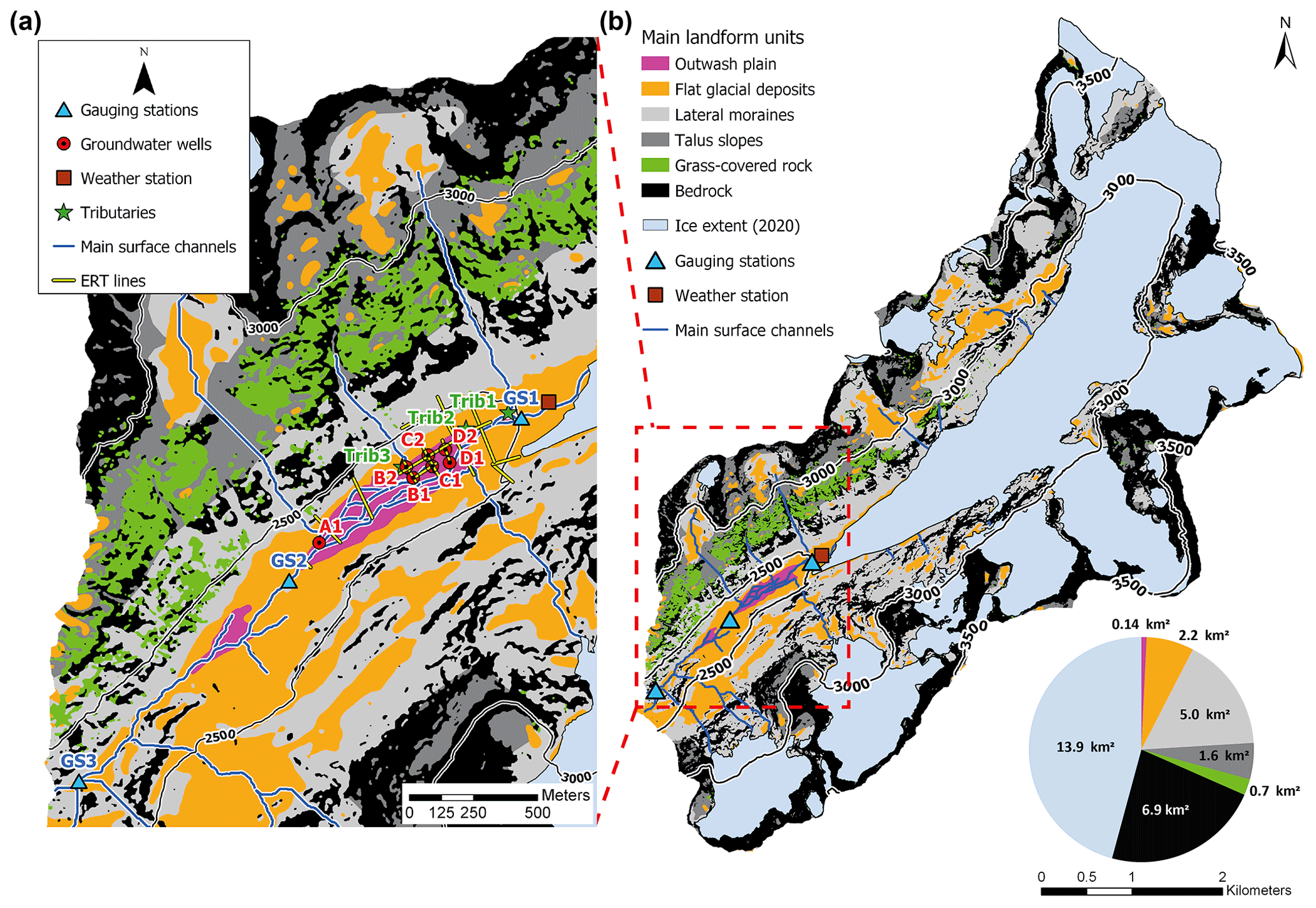
Figure 2 (a) The zoom-in window shows the field measurement stations installed between 2019 and 2021 as well as the ERT lines. The outwash plain is located between gauging stations 1 and 2 (GS1 and GS2). (b) Overview of the Otemma catchment classified based on its main geomorphological landforms (see Sect. 3.4). The pie chart shows the surface area of each unit.

A Tyrolean-type water intake (Lauterjung and Schmidt, 1989) has been constructed for hydropower production about 2.5 km downstream of the current glacier terminus and is used in the present study as the outlet of what we call the Otemma basin (Fig. 2b). It has an area of 30.4 km², a mean elevation of 3005 m a.s.l. (2350 to 3780 m) and a glacier coverage of 45 % in 2019 (adapted from GLAMOS, 1881–2020).

The geology of the underlying bedrock is composed of gneiss and orthogneiss from the Late Paleozoic Era with some granodiorite inclusions (Burri et al., 1999). The main geomorphological forms comprise bedrock, with some vegetation cover above the LIA limit (46 %), steep slopes (30 % post-LIA lateral moraines and 10 % talus slopes), gently sloping debris fans and morainic deposits (13 %) and a flat glaciofluvial outwash plain (0.9 %) (Fig. 2b). One main subglacial channel at the glacier snout provides water to a large, highly turbid and turbulent stream, which quickly reaches a flat outwash plain composed of sandy–gravelly sediments; this leads to a braided river network, which eventually converges in a more confined channel about 1 km downstream and extends to the hydropower intake. A few tributaries from small hanging glaciers or valleys also contribute to river discharge during the snow-free season.

2.2 Hydrometeorological data

In July 2019, we installed an automatic weather station (Fig. 2a) at the glacier snout at an elevation of 2450 m a.s.l., which recorded with a 5 min resolution air temperature, humidity, atmospheric pressure (Decagon VP-4) and liquid precipitation (Davis tipping rain gauge). After July 2020, total incoming shortwave radiation was also recorded by the device (Apogee SP-110). For the present analysis, winter solid precipitation data were provided by SwissMetNet, the Swiss automatic monitoring network, using information from the Otemma station (2.7 km from the glacier snout) or the Arolla station (10 km from the glacier snout). Data with a detailed description are available on Zenodo (Müller, 2022a).

2.3 Hydrological data

Hourly river stage was recorded from 2006 to 2018 at the water intake corresponding to the catchment outlet (GS3, Fig. 2a) by the local hydropower company (Force Motrice de Mauvoisin, FMM); corresponding discharge was estimated using a theoretical stage–discharge relationship provided by FMM. We post-processed the data by in-filling data gaps related to regular sediment flushing events (of duration <1 h) with linear interpolation. Winter discharge was also recorded, although a data gap usually occurred from October to December.

In August 2019, we installed three river gauging stations, one in the vicinity of the glacier snout (GS1), one at the end of the outwash plain (GS2) and one at the catchment outlet (GS3) (Fig. 2a). River stage, water electrical conductivity (EC) and water temperature were recorded continuously at 10 min intervals using an automatic logger (Keller DCX-22AA-CTD). Periodic EC and discharge measurements were also made in many tributaries and water sources, with a main focus on three representative tributaries along the outwash plain. Finally, we installed seven groundwater wells consisting of fully screened plastic tubes at an averaged depth of 1.5 to 2 m in the outwash plain, which covered four transects (A to D) perpendicular to the river in the direction of the base of the hillslope. Water table elevation was recorded in each well at a 10 min interval using SparkFun MS5803-14BA pressure sensors. Sensor bias was verified and corrected by bimonthly manual groundwater stage measurements. A more detailed description of the data is available on Zenodo (Müller and Miesen, 2022).

2.4 Electrical resistivity tomography

Electrical resistivity tomography (ERT) was used to map the sediment structure in the outwash plain. We performed a total of 21 lines from 2019 to 2021 using a Syscal Pro Switch 48 from Iris Instruments (Fig. 2a). The electrode array consisted of 48 electrodes with a spacing between 1.5 and 4 m, and dipole–dipole (DD) and Wenner–Schlumberger (WS) schemes were systematically used for better data interpretation. We processed the data using the open-source pyGIMLi python library (Rücker et al., 2017). All data inversions were calculated using a robust scheme (L1 norm) with different regularization strength (lambda from 1 to 100) to assess overfitting and underfitting. The depth of the outwash plain sediments was estimated by performing multiple transects in different parts of the outwash plain and by identifying the transition from water-saturated sediments with a resistivity value between 500 and 2000 Ω m and the bedrock layer with a resistivity of 4000 to 7000 Ω m, similar to other studies (e.g., Langston et al., 2011; Harrington et al., 2018). More detailed information on the data, results, codes and maps is available on Zenodo (Müller, 2022c).

3 Data analysis methods

In this study we used two frameworks based on recession theory to analyze both the catchment-scale hydrological response and the response of individual landforms. These two approaches were applied to our case study in the Swiss Alps using various field data, and we ultimately compare the results obtained from both methods together and against field observations. The workflow of the overall methodology is summarized in Fig. 3.

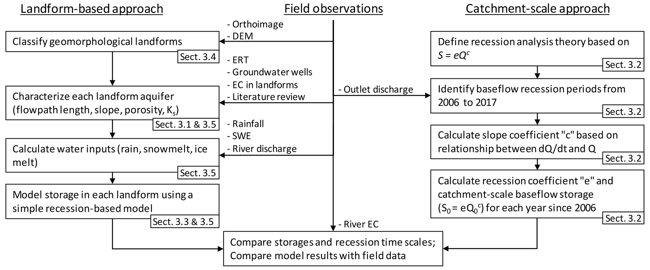
Figure 3 Sketch of the adopted workflow, separated between field observations and landform-based and catchment-based methods. The corresponding sections in the methodology are also highlighted. All abbreviations are detailed in the text.

3.1 Estimation of hydraulic conductivity in the outwash plain

While some literature exists to characterize most geomorphological landforms in glaciated catchments, data on post-LIA outwash plains in Alpine environments are scarce. We therefore used two different methods to estimate the saturated hydraulic conductivity (K_s) of the outwash plain.

The first method applied the pressure wave diffusion method documented in the work of Magnusson et al. (2014). Given a certain hydraulic diffusivity (D), this method was used to relate the aquifer head variations (h) at a distance x from the stream to the diel stream stage cycles (h_x=0) generated by ice melt. It furthermore made use of a simplified 1D Boussinesq equation, where advective fluxes were neglected (Eq. 1). This procedure is only valid for relatively flat aquifers with a thick unconfined saturated layer and where evapotranspiration losses can be neglected (Kirchner et al., 2020), which makes this approach well-suited for high-elevation outwash plains. By comparing the phase shift (time lag) and the amplitude dampening between the river stage and the groundwater signals, the aquifer hydraulic diffusivity (D) was estimated and related to K_s using the aquifer thickness (B) and assuming that the specific yield (S_y) was similar to the aquifer porosity (Eq. 2).

$$\begin{array}{}\text{(1)}& {\displaystyle \frac{\mathit{\delta }h}{\mathit{\delta }t}}=D{\displaystyle \frac{{\mathit{\delta }}^{\mathrm{2}}h}{\mathit{\delta }{x}^{\mathrm{2}}}}\text{(2)}& {\displaystyle }D={\displaystyle \frac{K_{\mathrm{s}}B}{S_y}}\end{array}$$

For this analysis, we used the two upstream and downstream well transects (B and D; see Fig. 2a) for two periods: during high flow in mid-August 2019 and during a lower-flow period in mid-September 2019. An additional groundwater well “B3” on transect B was also used for this analysis. The 1D partial differential equation was solved using a central-differencing scheme in space and a Crank–Nicolson method in time, imposing the measured river stage variations as a boundary condition. Prior to solving the equation, both river stage and groundwater heads were detrended by substracting the linear trend of each dataset as suggested by Magnusson et al. (2014). We then calibrated the model parameter D using a Monte Carlo approach where we minimized the root mean square error and maximized the Spearman rank correlation between observed and modeled groundwater heads. Hydraulic conductivity was finally calculated based on the aquifer thickness estimated by ERT, and porosity was estimated by measuring saturated water content (Decagon 5TM) at five locations in the upper sediment layer.

A second independent estimation of the hydraulic conductivity was obtained with salt tracing, using ERT time lapse with a measurement cycle of about 30 min. We injected 3 kg of salt dissolved in 15 L of water in a 1 m-deep pit in the center of the outwash plain and recorded the timing of the passage of the salt plume at a downstream transect (distance 9.38 m) using ERT, similarly to the work of Kobierska et al. (2015a). We only installed one ERT line perpendicular to the groundwater flow consisting of 48 electrodes with a 1 m spacing. Hydraulic conductivity can be calculated by solving Darcy's law for the mean pore velocity as follows:

$$\begin{array}{}\text{(3)}& v_{\mathrm{p}}={\displaystyle \frac{K_{\mathrm{s}}}{{\mathit{\theta }}_s}}{\displaystyle \frac{\mathrm{d}h}{\mathrm{d}x}},\end{array}$$

where $\frac{\mathrm{d}h}{\mathrm{d}x}$ is the aquifer gradient, θ_s is the aquifer porosity and v_p is the mean pore velocity corresponding to the travel distance divided by the travel time of the center of gravity of the salt plume.

3.2 Catchment-scale recession analysis

We analyzed the storage–discharge relationship at the catchment scale by using a classical recession analysis during periods when both water inputs (snow, rain) as well as outputs (evapotranspiration) can be neglected, i.e., during periods when discharge is only related to aquifer storage (Kirchner, 2009; Clark et al., 2009). Following Kirchner (2009), we describe the recession behavior of the aquifer storage with a nonlinear storage (S)–discharge (Q) function,

$$\begin{array}{}\text{(4)}& S=e{Q}^c,\end{array}$$

whose derivative, using $\frac{\mathrm{d}S}{\mathrm{d}t}=-Q$, is given by

$$\begin{array}{}\text{(5)}& -{\displaystyle \frac{\mathrm{d}Q}{\mathrm{d}t}}={\displaystyle \frac{\mathrm{1}}{\mathrm{ce}}}{Q}^{(\mathrm{2}-c)}.\end{array}$$

This is usually summarized as $-\frac{\mathrm{d}Q}{\mathrm{d}t}=a{Q}^b$, where $a=\mathrm{1}/\mathrm{ce}$ is the recession coefficient and $b=\mathrm{2}-c$ is the slope coefficient (Santos et al., 2018). The release behavior of the catchment-scale storage was characterized by identifying zones where the slope of the relationship between the rate of change ($-\frac{\mathrm{d}Q}{\mathrm{d}t}$) and discharge (Q) is constant in the logarithmic scale, which allowed calculation of the slope coefficient b.

We performed the recession analysis for the 12-year period of discharge data provided by FMM at the catchment outlet (GS3). The recession periods were automatically selected by identifying periods where flow is constantly decreasing for at least 10 d and is extended until the first increase in flow. The discharge recession data were smoothed (moving average with a span of 50 % of a given recession period) to remove small step-like decreases or small drops due to sensor failures, so that only the averaged trends are analyzed. Finally, we plotted the relationship between ($-\frac{\mathrm{d}Q}{\mathrm{d}t}$) and discharge (Q), and we average the recession points from all years in bins with an equal number of points (we selected 100), as suggested in the work of Kirchner (2009), to which we apply a linear regression (nonlinear least squares method, MATLAB R2019a). This procedure allowed estimation of the slope coefficient b. Once b is identified, we fitted a power-law function on the raw discharge data (without any smoothing) for each winter recession, using the analytical solution of Eq. (5) in order to estimate the recession coefficient e. Finally, this allowed us to relate the maximum baseflow discharge Q₀ to the catchment-scale baseflow storage S₀ using Eq. (4).

3.3 Assessing the hydrological response based on aquifer characteristics and recession analysis

Similarly to the catchment-scale recession analysis, the same relationship between storage and discharge can be applied to specific landforms, which allows estimation of the rate of water storage and release in different parts of a glaciated catchment. For instance, the form of the water table in an aquifer can be linked to the shape and physical properties of the landform (Troch et al., 2013). Using some simplifications, the Boussinesq equation (Boussinesq, 1904) provides a physically based means of estimating the temporal variation of the aquifer table along a one-directional aquifer and thus allows estimation of discharge based on the groundwater gradient and physical properties of the aquifer (Harman and Sivapalan, 2009a). For flat aquifers with homogeneous conductivity, a slope b of 1.5 (c=0.5) is common for the late recession (Rupp and Selker, 2006). Here, an analytical solution of the Boussinesq equation was proposed, leading to the discharge solution (Wittenberg and Sivapalan, 1999; Rupp and Selker, 2005) shown in Eqs. (6) and (7).

$$\begin{array}{}\text{(6)}& {\displaystyle }S=e{Q}^{\mathrm{0.5}}\text{(7)}& {\displaystyle }{Q}_t=Q_{\mathrm{0}}(\mathrm{1}+\mathit{\alpha }t{)}^{-\mathrm{2}}\text{(8)}& {\displaystyle }\mathit{\alpha }={\displaystyle \frac{Q_{\mathrm{0}}^{\mathrm{0.5}}}{e}}\approx {\displaystyle \frac{K_{\mathrm{s}}{h}_m}{\mathit{\varphi }{L}^{\mathrm{2}}}}\end{array}$$

A physical description of α was proposed (Eq. 8) based on the aquifer conductivity (K_s) and porosity (ϕ), the aquifer length (L) and the aquifer thickness at distance L (h_m) (Dewandel et al., 2003; Rupp and Selker, 2005; Stewart, 2015).

In the case of a significantly sloping aquifer ($>{\mathrm{10}}^{\circ }$), a value b=1 is usually proposed for the late drainage (Rupp and Selker, 2006; Muir et al., 2011). In this case, if the aquifer thickness was small enough, the aquifer flux would be mostly advective and conducted by the bedrock slope (Harman and Sivapalan, 2009b), so that discharge recession becomes linear (Eqs. 9 and 10). Due to the nonlinearity of the Boussinesq equation, the parameter α could only be approximated using numerical linearization approaches (Hogarth et al., 2014; Verhoest and Troch, 2000). In this study we used one of the simplest proposed descriptions for α (Eq. 11), similar to the previous one, where only $h_m/L$ (the aquifer slope) is replaced by sin (θ) and θ is the bedrock slope (Harman and Sivapalan, 2009a; Berne et al., 2005; Rupp and Selker, 2006).

$$\begin{array}{}\text{(9)}& {\displaystyle }S=eQ\text{(10)}& {\displaystyle }{Q}_t=Q_{\mathrm{0}}{e}^{-\mathit{\alpha }t}\text{(11)}& {\displaystyle }\mathit{\alpha }={\displaystyle \frac{\mathrm{1}}{e}}\approx {\displaystyle \frac{K_{\mathrm{s}}\sin \left(\mathit{\theta }\right)}{\mathit{\varphi }L}}\end{array}$$

In both equations (Eqs. 7 and 10), the rate of aquifer decline can be related to a recession constant ($\mathrm{1}/\mathit{\alpha }$), corresponding to the characteristic response time of the aquifer. Based on this approach, we reviewed the range of estimated hydraulic conductivity values reported in recent studies for typical landforms in glaciated catchments. Combined with realistic aquifer properties (slope, porosity, aquifer length) for each type of landform, we applied the proposed relationships for flat (Eq. 8) or sloping aquifers (Eq. 11) and finally assessed the recession timescales ($\mathrm{1}/\mathit{\alpha }$) at which different storage compartments provide water for baseflow.

3.4 Superficial landform classification

Landform classification was performed by combining a visible band orthoimage from 2020 with a 10 cm resolution (SwissTopo, 2020) and a 2 m resolution digital elevation model (DEM) (SwissTopo, 2019). We calculated the slope from the DEM and classified it in categories as suggested in the work of Carrivick et al. (2018): $<{\mathrm{8}}^{\circ }$ for outwash plains; 8–22^∘ for mildly sloping glacial deposits and debris cones; 22–42^∘ for lateral moraines below the LIA limit and talus slopes above the LIA limit; $>{\mathrm{42}}^{\circ }$ for bedrock. We then downscaled the orthoimage to 2 m and combined the RGB bands with an additional band corresponding to the slope classes. We manually identified small zones corresponding to the main landform features and performed a supervised classification using a random tree classifier (ArcGIS Pro v2.3). We finally calculated the median class for a moving window of 10 cells by 10 cells (20×20 m) to smooth out noise in the results. A specific class for grass was used, since many grass patches were identified above the LIA line on shallow soils on top of bedrock. Lateral moraines below the LIA line were distinguished from coarser debris talus slopes with similar slopes in zones where glaciers were absent during the LIA. The glacier extents from 1850 (LIA limit) and 2016 are provided by the Swiss Glacier Inventory 2016 (Linsbauer et al., 2021). The results are presented in Fig. 2b.

3.5 Landform-based model of the hydrological response of single geomorphological units

Based on the previously discussed recession theory (Sect. 3.3), we propose a simple methodology to estimate the seasonal storage and discharge contribution of each individual superficial landform storage compartment in the Otemma catchment. In order to estimate the maximum water storage, we used the total area (A_i) of each classified landform (Sect. 3.4) and an estimation of their sediment thickness, similarly to other studies (Hood and Hayashi, 2015; Rogger et al., 2017). Sediments are however never fully water-saturated, so that it remained difficult to estimate the maximum aquifer thickness for each landform. To overcome this limitation, we defined a simple hydrological model where we simulated a realistic daily water input (Q_in) in the form of rain (P_rain) and snowmelt (P_snow) and estimated storage (S) and outflow discharge (Q_out) based on the nonlinear storage–discharge relationship (Eq. 4). We defined c based on the landform slope and estimated e following Eq. (8) or (11) using realistic hydrological characteristics of each landform: hydraulic conductivity was based on our measurements (Sect. 3.1) or from a review of the literature, while the aquifer slope and length were estimated for each landform based on our landform classification by manually measuring the averaged landform length (Fig. 2b).

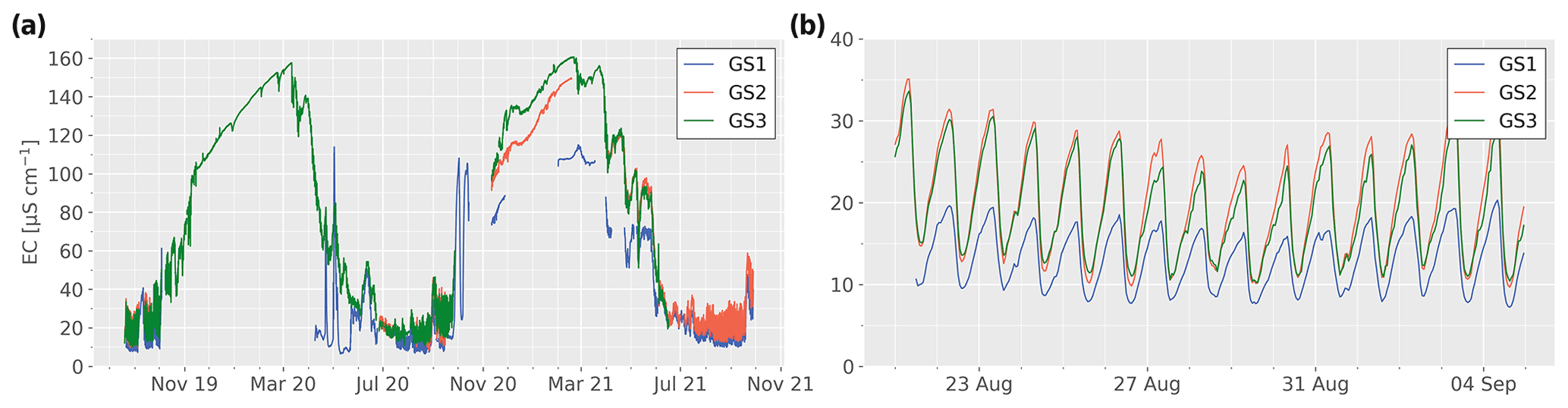
Figure 4 (a) Streamflow electrical conductivity (EC) at the three gauging stations (GS1 to GS3) during 2 years. (b) Zoom-in window showing the EC for the first 20 d of measurement. Large gaps in winters are due to sensor failures.

Following this approach, we defined Eqs. (12) to (14) in order to simulate the seasonal storage and discharge over a whole year.

$$\begin{array}{}\text{(12)}& {\displaystyle \frac{\mathit{\delta }{S}_t}{\mathit{\delta }t}}=Q_{\mathrm{in},\mathrm{t}}-Q_{\mathrm{out},\mathrm{t}},\text{(13)}& {\displaystyle }{Q}_{\mathrm{in},\mathrm{t}}=\left(\left(P_{\mathrm{snow},\mathrm{t}}+P_{\mathrm{rain},\mathrm{t}}\right)A_i+Q_{\mathrm{glacier},\mathrm{t}}\right)/A_{\mathrm{catchment}},\text{(14)}& {\displaystyle }{Q}_{\mathrm{out},\mathrm{t}}={\left({\displaystyle \frac{S_t}{e}}\right)}^{\mathrm{1}/c},\end{array}$$

where $\frac{\mathit{\delta }S}{\mathit{\delta }t}$ is the change in storage in mm d⁻¹, Q_in,t is the daily water input at time t and Q_out,t is the generated daily output discharge based on the nonlinear storage–discharge equation. P_snow and P_rain are the daily snowmelt and daily liquid precipitation in mm d⁻¹, A_i is the area of each landform, Q_glacier is the daily river discharge from the glacier in L d⁻¹ and A_catchment is the total catchment area in square meters. Finally, e is the recession parameter estimated based on α (Eq. 8 or 11) and c the slope coefficient (1 for slopping aquifers $>{\mathrm{10}}^{\circ }$ and 0.5 for flatter aquifers). In these equations, the landform storage (S_t) was scaled by dividing the volume by the entire catchment area, which allowed ready comparison of the storage associated with each landform.

The snowmelt input was modeled with a snow accumulation routine (rain transitions to snow from an air temperature between 1 and 2 ^∘C) and a degree-day model for daily snowmelt estimation following Gabbi et al. (2014), with a degree-day melt factor of 6.0 mm ^∘C⁻¹ d⁻¹ when air temperature is higher than 1 ^∘C. The catchment was separated into 50 m elevation bands with a calibrated temperature lapse rate of 0.5 ^∘C 100 m⁻¹ and a precipitation lapse rate of +10 % 100 m⁻¹. Winter precipitations from SwissMetNet were adapted using a correction factor for each year. The melt parameters, precipitation correction factor and lapse rates were estimated by minimizing the error between modeled and observed snow water equivalent (SWE) based on 92 snow depth measurements and two snow pits for density measurements made near the maximum snow accumulation on 28 May 2021. It was further calibrated by matching the snowline limit during the snowmelt season as suggested in Barandun et al. (2018), based on daily 3 m resolution Planet images (Planet Team, 2017). Snowmelt and rain inputs were considered to recharge entirely the whole aquifer (no surface flow), and there was no routing or water exchange between the different landforms, so that our estimates represent the maximum potential storage linked to a realistic maximum recharge.

In the case of the outwash plain, an additional glacier melt input (Q_glacier) was provided, since this is the only landform directly recharged by the river network in Otemma. Only a small fraction of the total river discharge was allowed to recharge the outwash plain aquifer. An infiltration rate of 100 L s⁻¹ (2 % of mean summer discharge) from May to October was used, estimated from dilution gauging along the stream and preliminary modeling results. This amount was also found to realistically approximate the rate of recharge observed using the groundwater wells. Finally, the maximum storage (sediment thickness) of the reservoirs cannot be exceeded in any landform.

Based on the three sources of water (rainwater, snowmelt, glacial stream), a small routine was also added to calculate the source water partitioning in each landform. At each time step, the reservoir was assumed to be fully mixed and a water amount for each water source was removed, proportional to the estimated partitioning at the previous time step and so that the total water removed equates the calculated discharge (Q_out,t). The amount of water recharge from each source is then added, and a new partitioning is calculated. This allowed tracking of the seasonal contribution of different water sources in each landform.

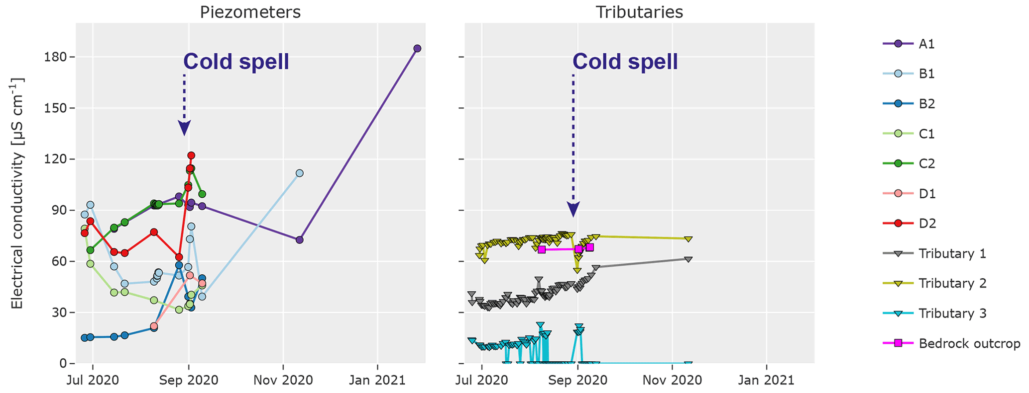
Figure 5 Temporal evolution of EC at seven wells (A1 to D2) in the outwash plain, in three tributaries as well as one bedrock spring (see Fig. 2a for the location). Values of 0 for tributary 3 indicate no surface flow. A cold spell resulting in snowfall over the whole catchment is indicated by the dark blue arrow.

4 Results

4.1 Water electrical conductivity

4.1.1 Stream observations

Streamflow EC in the Otemma catchment shows strong seasonal and diel cycles driven by snowmelt and glacier melt (Fig. 4). During summer, when discharge is highest, streamflow EC remains very low, with small diel variations on the order of 10 to 20 µS cm⁻¹ (Fig 4b). During this period, EC is strongly negatively correlated with river discharge, with maximum streamflow EC in the morning. There is an EC increase between the glacier snout (GS1) and the end of the outwash plain (GS2) but little change further downstream. Indeed, during summer high flow, the EC difference between GS2 and GS3 is very limited, with EC at GS3 consistently smaller by a few µS cm⁻¹ in the morning when EC is maximal. This decrease is likely due the contribution of the two main surface tributaries fed by ice melt from the southwestern-most hanging glacier (see Fig. 2), where water is characterized by low EC. Additionally, this very limited change in EC could indicate little contribution from groundwater with higher EC in this zone compared with the larger increase in EC observed in the outwash plain region (GS1 to GS2).

After November, EC increases gradually during the whole winter (Fig 4a), until the first onset of snowmelt in early spring. Similar to the summer, there is a difference in EC between GS1 and GS2, which becomes larger as EC at GS1 increases less rapidly in March 2021. A small EC difference between GS2 and GS3 only occurs during the very low-flow conditions from mid-November to March. This EC increase suggests that, during winter, the contribution of ice melt from the hanging glaciers is likely very limited, so that some groundwater contributions from the hillslopes become dominant and contribute to increasing the stream EC between GS2 and GS3. The change appears however smaller than between GS1 and GS2, suggesting less groundwater contribution in this zone, similar to the observation in the summer.

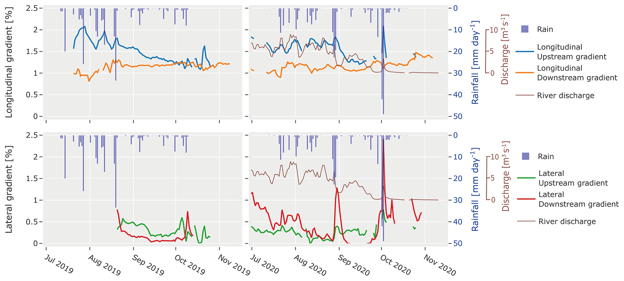
Figure 6 Groundwater gradients in the outwash plain for summers 2019 and 2020. The upstream longitudinal gradients are estimated between wells D1 and C1, the downstream gradient between C1 and B1. The lateral gradients are estimated between D wells upstream and B wells downstream, and their slope is directed towards the main river. In 2020, the mean daily discharge at the glacier outlet (GS1) is shown in brown and was scaled between 1 % and 2 % slope for easier comparison with the gradients. Daily measured rainfall at the glacier snout (weather station) are shown by inverted blue bars.

4.1.2 Hillslope and groundwater observations

We monitored the EC of selected landforms as well as of different water sources. The averaged snowmelt EC was 5.1±2.5 µS cm⁻¹ based on 28 snowpack samples collected during the snowmelt season in the outwash plain and on the glacier surface up to 2850 m a.s.l. Surface ice-melt samples show EC values of 5.7±4.3 µS cm⁻¹ based on 29 samples. The average rain EC value is 31.6±11.3 µS cm⁻¹ based on 11 samples. The reason for a slightly higher EC in rain than snowmelt is not known but has also been reported in other studies (Zuecco et al., 2019).

Tributaries on the side of the outwash plain show only limited change in EC during summer (Fig. 5) but present different trends. Tributary 1 is located below a hanging valley, likely containing buried ice or permafrost and snow at high elevation, leading to a perennial superficial flow. The relatively low EC of this tributary seems to indicate a marginal groundwater contribution, with probably only a short contact time between the morainic material and meltwater in the higher part of the catchment. Tributary 2 exfiltrates from sediments at the base of the lateral moraine, and its EC is only slightly higher than the bedrock exfiltration, suggesting that this tributary is mainly fed by water stored in the bedrock which infiltrates in the coarse sediments of the lateral moraine and re-emerges at the base of the outwash plain. During a cold spell (30 August), accompanied by a heavy rain event (42 mm) on the preceding day, a small drop in EC in tributary 2 can be observed and is likely related to an increased water storage in the lateral moraines, which empties in a few days. Tributary 3 maintains low EC close to the value of snowmelt and becomes dry in August, indicating its direct dependence on snowmelt transmitted by overland flow with hardly any contact time with the sediments.

The EC measured in the groundwater wells shows much stronger variations, both spatially and temporally (Fig. 5). In the upper part of the outwash plain (wells B, C, and D), groundwater EC near the stream is low and similar to the stream EC, indicating strong stream infiltration to the outwash plain. Near the hillslopes, EC is higher and also larger than the tributaries, indicating either contribution from deeper hillslope exfiltrations with higher EC or river contribution with long flowpaths from the stream network. During the cold spell, river discharge decreased and groundwater EC became larger in C2 and D2, likely due to decreased infiltration from the river and an increased influence from a deeper groundwater source. Well A1 shows a smoother signal, with high values year-round and a gradual increase in summer, likely due to the decreasing snowmelt contribution in the outwash plain. During winter, groundwater EC in well A1 increases, rapidly reaching 180 µS cm⁻¹.

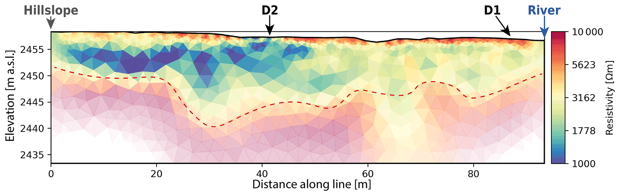
Figure 7 Results of one ERT profile perpendicular to the stream at the location of groundwater wells D1 and D2 (see Fig. 2). The electrode array consists of 48 electrodes with 2 m spacing. Robust inversion was performed for the dipole–dipole scheme using a regularization coefficient lambda of 10. Location of groundwater wells as well as the hillslope and river sides are also highlighted. The red dashed line shows the limit between water-filled sediments and the underlying bedrock.

4.2 Groundwater dynamics in the outwash plain

From the groundwater head observations in the outwash plain, we computed the daily averaged lateral (perpendicular to the stream) and longitudinal (parallel to the stream) aquifer gradients (Fig. 6). During the summer, the lateral upstream gradient (well D1–D2) is mostly comprised between 0 % and 0.5 %. The EC at well D2 is similar to tributary 2, which suggests a hillslope recharge from tributary 2 or a constant deeper bedrock exfiltration which maintains a mild lateral gradient towards the stream. The lateral downstream gradient (wells B1–B2) shows a stronger slope of about 1 % in the direction of the stream, which gradually decreases to values close to 0 % by September. This gradient seems closely related to the snowmelt-fed tributary 3. Indeed, well B2 shows a low EC in the early melt season, similar to tributary 3, which only increases in mid-August, when this tributary runs dry (Fig. 5).

The longitudinal gradient seems to maintain a larger slope of about 1 % to 2 % during the summer. Interestingly, the daily discharge in 2020 shows a similar weekly dynamic to the upstream gradient, although the gradient tends to react with a delay of 1 to 2 d. This suggests a strong influence of the stream discharge magnitude on the upstream gradient, which starts decreasing only in early September, i.e., at the moment when discharge peaks decrease.

River stages at the well transects could not be measured continuously due to the high discharge and unstable sediments; a few isolated measurements show that, in the upper part of the floodplain (B, C, and D transects), the river stage is always 10 to 40 cm higher than the groundwater level in the wells closest to the river, indicating a lateral gradient from the stream to the well and thus a losing stream reach. Higher discharge therefore leads to a higher river stage, which increases the hydraulic gradient through the riverbed and therefore promotes higher stream infiltration.

Based on the hydraulic gradients, it appears that groundwater flows in the same direction as the terrain's main slope are recharged in its upstream part by the stream and re-emerge at the end of the outwash plain. This re-emergence results from the underlying bedrock with much lower hydraulic conductivity, which forces water to exfiltrate in the river as the sediment thickness decreases towards the end of the plain. This groundwater upwelling is also supported by the EC in well A1 (Fig. 5), which shows the highest EC in the floodplain, although it is located at 5 m from the river, indicating long flowpaths and no direct contact with the river at this location.

4.3 Hydraulic conductivity in the outwash plain

4.3.1 Pressure wave diffusion

We identified aquifer thickness using ERT and illustrate the results for well transects D1–D2 (Fig. 7). A thin layer of dry sediments can be identified at the top, following a lower layer where resistivity is in a range between 1000 and 3000 Ω m⁻¹. Near the stream, resistivity is slightly higher, likely due to lower groundwater EC close to the stream than the hillslope. The bedrock is located at a depth of about 10 to 15 m, with resistivity higher than 5000 Ω m⁻¹.

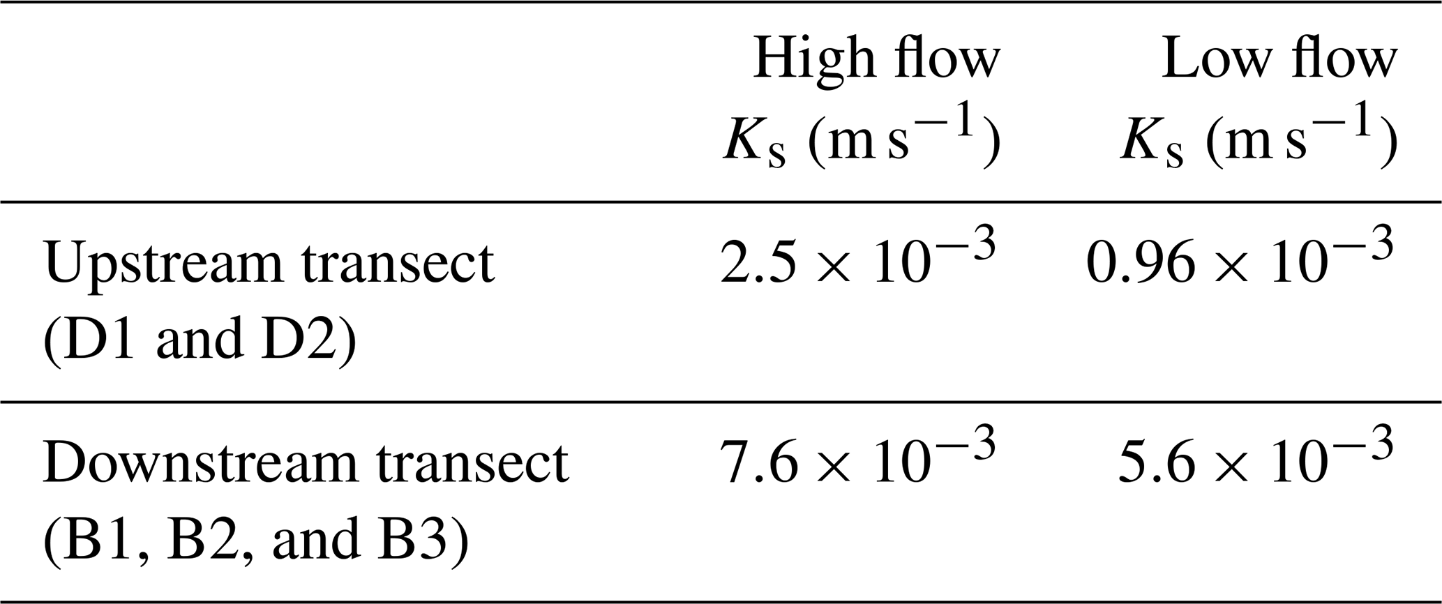
Using the diffusion model (Sect. 3.1), we modeled the diffusion of stream stage fluctuations in the aquifer, estimated diffusivity and obtained hydraulic conductivity using an aquifer thickness (15 m) and porosity, with an average value of 0.25. Unlike in the work of Magnusson et al. (2014), satisfying results were obtained using a unique K_s value to simulate the fluctuations of all wells along the same transect (Figs. A1 and A2). The results are summarized in Table 1. Only the estimated lower value for well transect D in September 2019 appears more uncertain, as the simulated head variations for well D1 at 5 m from the river do not match the observed results well (Fig. A2b).

Table 1 Estimated saturated hydraulic conductivity of the outwash plain for high-flow and low-flow conditions during the summer period along two transects based on the pressure wave diffusion model.

4.3.2 Salt tracer injection

The passage of the salt plume was identified by a change in resistivity (of more than an order of magnitude) in a well-constrained zone of the ERT line (plume radius of about 1 m), with the maximum change occurring 10.5 to 11.5 h after injection. Using a travel distance of 9.38 m, we obtain an average pore velocity v_p of $\mathrm{2.4}\times {\mathrm{10}}^{-\mathrm{4}}$ m s⁻¹. The corresponding aquifer gradient between three groundwater wells (one 1 m upstream of the injection point and two along the ERT line) has a maximum slope of 1.7 %. Based on these values, we obtain an estimated hydraulic conductivity of $\mathrm{3.5}\times {\mathrm{10}}^{-\mathrm{3}}$ m s⁻¹. A detailed illustration of the time-lapse ERT is available on Zenodo (Müller, 2022c). The surface hydraulic conductivity estimated with this second approach is close to the mean of the K_s values estimated with the diffusion model ($\mathrm{4.2}\times {\mathrm{10}}^{-\mathrm{3}}$ m s⁻¹).

4.4 Landform-based groundwater storage dynamics

Clow et al. (2003)Caballero et al. (2002)Muir et al. (2011)Kurylyk and Hayashi (2017)Caballero et al. (2002)Rogger et al. (2017)Langston et al. (2013)Magnusson et al. (2012)Kobierska et al. (2015a)Winkler et al. (2016)Rogger et al. (2017)Harrington et al. (2018)Harrington et al. (2018)Robinson et al. (2008)Ó Dochartaigh et al. (2019)Käser and Hunkeler (2016)

Table 2 Calculation of the recession constant $\mathrm{1}/\mathit{\alpha }$ for different landforms based on a typical aquifer structure ($h_L/L$, ϕ, and L) and a review of hydraulic conductivity values (K_s) reported in proglacial studies. Maximum and minimum values of K_s are given where applicable. Values of $\mathrm{1}/\mathit{\alpha }$ for studies which estimated this parameter based on discharge recession analysis independently of K_s were also reported.

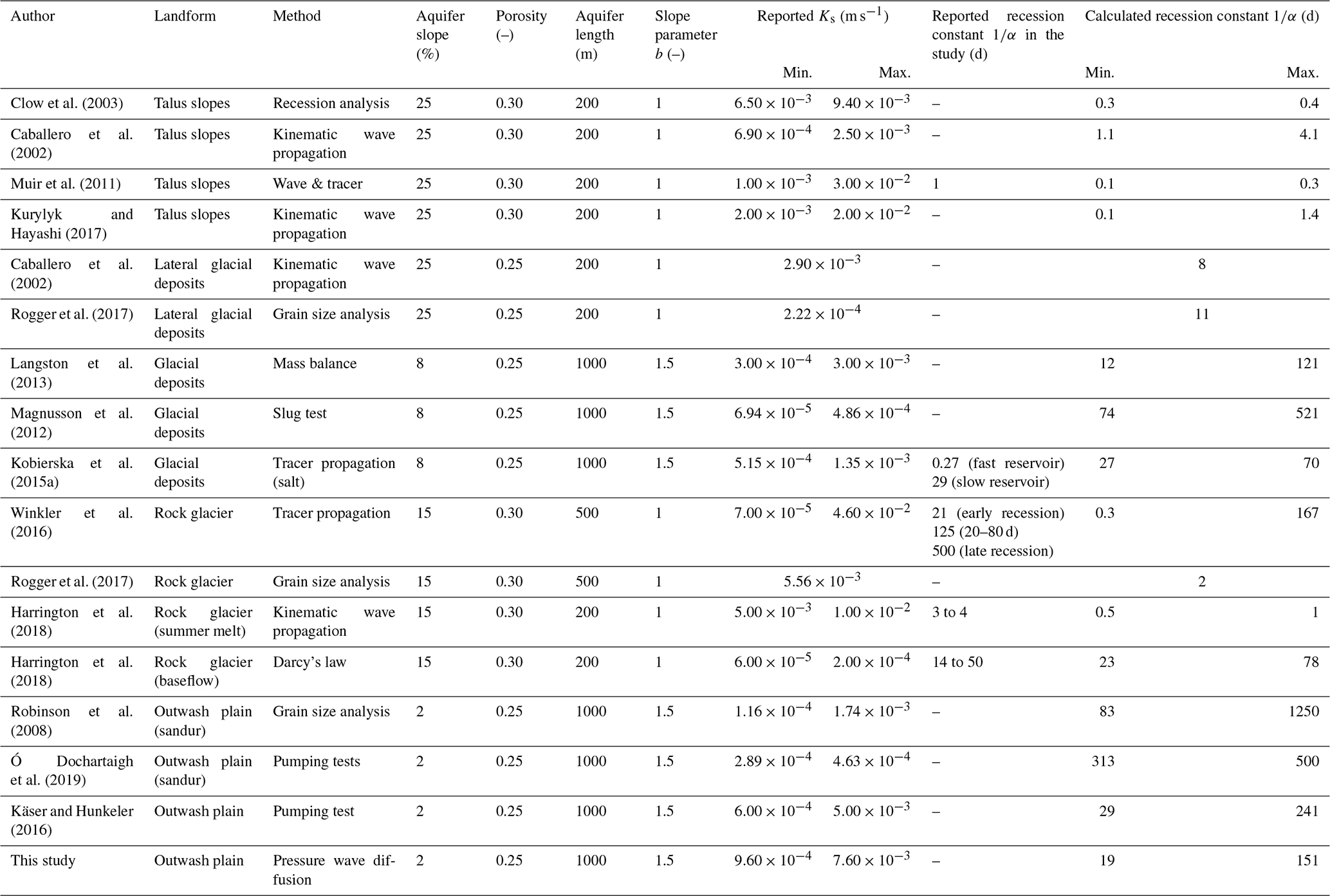
In order to disentangle the relative contribution of different superficial landforms, we suggest comparing the recession constant ($\mathrm{1}/\mathit{\alpha }$), which provides a way to compare how fast each aquifer compartment releases water and what their significance is for maintaining flow during dry periods. We reviewed studies focusing on specific landforms in glaciated catchments where hydraulic conductivity (K_s) was estimated in Table 2.

We then estimated the storage and response time of each unit in the Otemma catchment using the landform-based model (Sect. 3.5) based on K_s values from Table 2, including maximum and minimal K_s values to account for uncertainty. We also defined aquifer properties realistic for our catchment (Table 3). For lateral moraines (Caballero et al., 2002; Rogger et al., 2017), we selected K_s to be smaller than for flatter deposits (Kobierska et al., 2015a), which probably reflects the lesser degree of compaction at the valley bottom. We separated talus slopes from lateral moraine as talus slope material is coarser and lay above the LIA line. For the outwash plain, we used our own estimate of the hydraulic conductivity, and for mildly sloping glacial deposits, comprised between a slope of 8 to 22^∘, we used a mean slope of 10^∘ as the majority of those deposits were rather flat.

Table 3 Estimated recession constant ($\mathrm{1}/\mathit{\alpha }$) based on aquifer characteristics of the entire Otemma catchment for the main landform compartments. c stands for the slope coefficient of Eq. (4) and was defined as 1 when the aquifer slope is larger than 10^∘.

Supported by a simple degree-day model for snow accumulation and melt, we estimated the catchment-scale average rainfall and snowmelt during the year 2020. Rainfall amounts to a total of 204 mm and snowmelt to 1732 mm of water equivalent (see Fig. 8a). Figure 8b shows the resulting estimated maximum storage for each landform.

Figure 8 (a) Measured precipitation input at the glacier snout (mm d⁻¹) and mean snowmelt input simulated with a simple degree-day approach (mm d⁻¹). (b) Evolution of the groundwater storage of the four main geomorphological landforms (outwash plain; flat glacial deposits $<{\mathrm{22}}^{\circ }$; lateral moraines $>{\mathrm{22}}^{\circ }$; talus slopes $>{\mathrm{22}}^{\circ }$) based on the landform model described in Eqs. (12) to (14). Storage volumes in cubic meters are divided by the entire catchment area in square meters to provide comparable estimates in millimeters.

The resulting maximum baseflow storage in the flat glacial deposits is 19 mm (with an uncertainty margin from 13.5 to 32.5 mm) or a maximum aquifer thickness of 1.1 m (0.8 to 1.8 m) during peak snowmelt. The storage in the outwash plain gradually increases due to constant recharge from the river and rapidly reaches its maximum storage of 11.3 mm (or an aquifer thickness of 10 m). The lateral moraines show a very flashy storage response linked to their short recession constant. Their storage reaches 23 mm (15 to 52 mm) during snowmelt, corresponding to an aquifer thickness of 0.55 m (0.35 to 1.25 m). Due to their very low retention capacity, talus slopes only transmit water, and their storage is low, with only 1.8 mm (1 to 4.5 mm) and a maximum aquifer thickness of 0.11 m (0.06 to 0.27 m). After peak snowmelt, storage decreases quickly in the lateral moraines and somewhat more slowly in the flatter glacial deposits, while maximum storage is maintained in the outwash plain due to the stream recharge. During fall, lower discharge leads to a storage decrease in the outwash plain too, so that by early December the total remaining storage becomes very limited, with only 8.8 mm (5 to 20 mm) remaining from the outwash plain and flat moraine deposits.

4.5 Catchment-scale winter river recession analysis

Discharge recession was analyzed from 2006 to 2017 at the catchment outlet by calculating the averaged relationship between recession rates ($\mathrm{d}Q/\mathrm{d}t$) and river discharge (Q) (Fig. 9). A change in slope occurs for discharge higher than 0.33 mm d⁻¹, probably due to the transition between discharge dominated by ice melt to discharge fed by groundwater. Due to this slope change, we assume that the recession starts when baseflow discharge is smaller than 0.33 mm d⁻¹, and higher values are excluded for the linear regression shown in Fig. 9.

Figure 9 Plot of the smoothed discharge recessions ($-\mathrm{d}Q/\mathrm{d}t$) against discharge (Q) for all recession periods from 2006 to 2017 (in grey) at the catchment outlet (GS3). Binned averages are shown in red, each bin comprising 1 % of the data points. A linear regression (in the logarithmic space) to all binned values smaller than 0.33 mm d⁻¹ is plotted in blue. Axes are in logarithmic scale.

Figure 10 Annual recession analysis at the catchment outlet (GS3). The measured discharge is presented in blue (logarithmic scale), and the best fit of the power-law regression ($Q_t=Q_{\mathrm{0}}(\mathrm{1}+\frac{\mathrm{1}}{e}{Q}_{\mathrm{0}}^{\mathrm{0.5}}t{)}^{-\mathrm{2}}$) is shown in red, along with the estimated fitted parameters Q₀ and e. Day of year larger than 365 indicates a recession spanning over the following year. The years 2010 and 2017 show large data gaps, so that no fit was calculated.

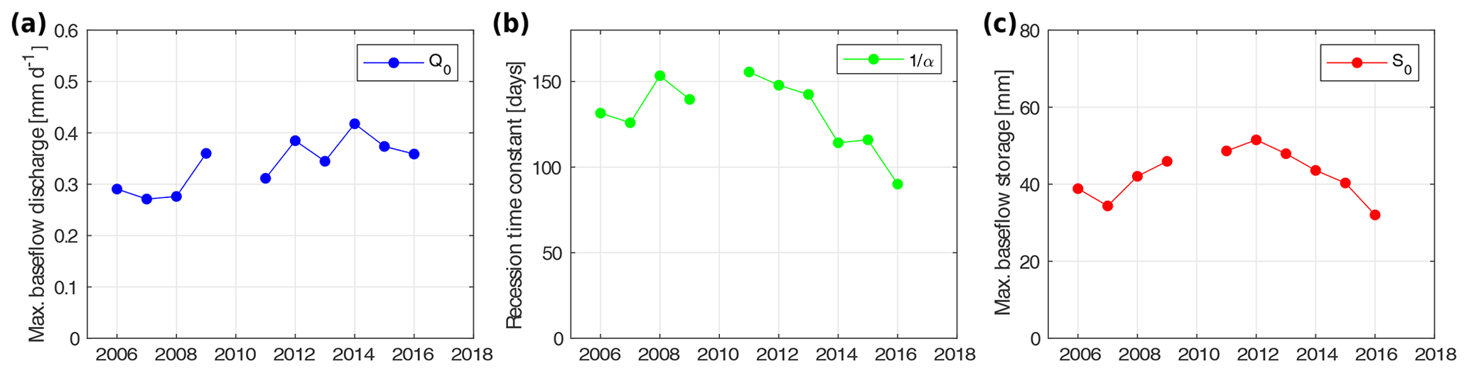
Figure 11 Temporal evolution of the recession characteristics obtained from the annual recession analysis of the Otemma catchment, showing the results of the best-fitted parameters for (a) maximum baseflow (Q₀), (b) recession constant ($\mathrm{1}/\mathit{\alpha }$), and (c) maximum baseflow storage (S₀).

The estimated regression has a slope of b=1.56, leading to a quadratic relationship between storage and discharge (Eq. 6). Due to the low values computed in Fig. 9, a change in the smoothing process of the raw discharge data may have an impact on the recession. We have tested different processing parameters and assessed the impact on the linear regression; overall, the slope varies between 1.45 and 1.65.

Using the same recession periods, the recession trends of each individual year are assessed (Fig. 10) using a quadratic relationship (Eq. 8) and fitting the maximum baseflow discharge (Q₀) and the recession coefficient (e). The corresponding calculated recession constant ($\mathrm{1}/\mathit{\alpha }$) seems to decrease in recent years, but the trend is unclear due to the overall short time period, while the temporal evolution of Q₀ and S₀ does not show any trend, suggesting no clear increase in groundwater storage over the 12-year period (Fig. 11).

Overall, we obtain a similar estimation of the baseflow storage in the Otemma catchment during each winter, with a mean maximum baseflow discharge of 0.34 mm d⁻¹, a mean maximum storage of 42.5 mm and a recession constant ($\mathrm{1}/\mathit{\alpha }$) comprised between 90 and 155 d. Finally, at the end of the recession periods in late winter, discharge has decreased by a factor of 3, which indicates that the baseflow storage does not completely empty and still retains on average 58 % of the maximum baseflow storage of early December.

Those results are in contradiction with the landform-based model (Fig. 8), where a maximum baseflow storage during early December was estimated to only 8.5 mm. Accordingly, the landform-based analysis seems to miss a relatively important storage compartment.

5 Discussion

5.1 Groundwater storage and release functions of the main geomorphological features

Our analysis has shown that the landform- as well as catchment-scale hydrological responses critically depend on (i) the sediment structure defining K_s and (ii) the landform characteristics in terms of slope and aquifer flowpath length. These key properties can then be combined to estimate an averaged response time ($\mathrm{1}/\mathit{\alpha }$) of each landform, although the storage–release behavior may be more complicated when considering more complex aquifer geometries (Berne et al., 2005), heterogeneous landforms with varying physical properties for K_s and ϕ, preferential flowpaths (Harman et al., 2009) or non-stationary processes (Benettin et al., 2017). In this study, we focused on characterizing the “slow” groundwater compartment, which is relevant for baseflow only, but an initial part of the water release may also occur in a faster superficial layer, as suggested in other studies (e.g., Winkler et al., 2016; Kobierska et al., 2015b; Stewart, 2015). Our approach, while simple, relies on physical properties of the aquifer. The calculated values for $\mathrm{1}/\mathit{\alpha }$ were similar to studies which estimated this parameter based on direct observations of discharge recession. This supports the validity of our approach for analyzing the storage–release behavior and the relative importance of different landform units in a glaciated catchment.

With this analysis, we have shown that only flat aquifers release water at timescales longer than weeks. In addition to K_s, the bedrock slope plays an important role, as it changes the relationship between storage and discharge, illustrated in our landform-based model by the slope coefficient c. Indeed, steeper slopes promote stronger advective fluxes (Harman and Sivapalan, 2009a) and modify the recession equation (Eqs. 7 and 10), so that a sloping aquifer (c=1) would lose 50 % of its storage 1.4 times faster and 99 % 4.5 times faster than a flat aquifer (c=0.5).

The seasonal landform-based analysis of superficial storage proposes an example of the groundwater dynamics in a glaciated catchment. The estimated storage amounts are likely not accurate due to a strong simplification of the recharge processes and the absence of superficial overland flow; it nevertheless illustrates (i) the strong relationship between recharge and storage, (ii) the importance of the timing of the water input and (iii) the relative speed at which different reservoirs may empty. Accordingly, we can establish a sound perceptual model (see Sect. 5.3).

Prior to introducing this model, we first discuss and summarize hereafter what new insights we gain from our case study on the hydrological functioning of the main classes of geomorphological landforms.

5.1.1 Talus slopes

In the Otemma catchment, talus slopes have only a marginal extent, so that the estimated storage is very low. In other less glaciated catchments, talus slopes may cover a much larger area, but, due to their coarse aquifer structure, their recession constant is only on the order of a day (Table 2), leading to a rapid transmission of water and little storage capacity. This is illustrated in our landform-based model by a maximal aquifer thickness of 11 cm. Therefore, groundwater storage is likely discontinuous and may only occur in pockets due to bedrock depressions at the base of the talus (fill and spill mechanism; Tromp-Van Meerveld and McDonnell, 2006; Muir et al., 2011). If a less conductive layer exists at the bottom of the talus, most studies have only reported a few centimeters of water saturation with relatively high conductivity (Muir et al., 2011; Kurylyk and Hayashi, 2017). Some studies have however shown different results, mainly the study by Clow et al. (2003), who estimated an aquifer thickness of a few meters and concluded that talus slopes contributed up to 75 % of winter baseflow. We want to stress here that this study is based on an erroneous calculation of the storage–discharge relationship where the authors wrongly included the time. This mistake may have influenced the conclusions made by others, and we insist here that talus slopes do not have the capacity to store water; they only transmit it from and to other landforms or the underlying fractured bedrock, as also suggested by others (e.g., McClymont et al., 2011; Harrington et al., 2018).

5.1.2 Steep lateral moraines

Steep lateral moraines may present glacial deposits on the order of tens of meters (Rogger et al., 2017) and have a lower hydraulic conductivity than talus slopes. Even though their structure is steep, they may retain water at a timescale of around 1 week. Their response remains relatively flashy, and the amount of potential storage is mainly driven by the rate of snowmelt in the early summer season. This is illustrated in our field observations in early September 2020, where the EC in tributary 2 recovers rapidly after a heavy rain event (Fig. 5) and where the lateral downstream gradient decreases on the same timescale (Fig. 6). Additionally, EC difference between the bedrock outcrop and tributary 2 is marginal, indicating limited chemical weathering and thus fast subsurface flow.

In our landform-based model, we assumed a homogeneous recharge, which is unlikely in the late mid-summer season, when snowmelt mainly occurs in the upper part of the catchment or in hanging valleys and when both surface and subsurface meltwater responsible for its recharge are likely concentrated in gullies or other zones of flow convergence due to the bedrock topography. The amount of recharge of steep lateral moraines is thus likely dependent on the frequency of flow convergence upslope; the more concentrated the upslope flow is, the less recharge occurs. In Otemma, these concentrated flows seem rather superficial, with limited infiltration into deeper parts of the moraine, which is likely due to more cemented grains and early soil development. Part of the water does nonetheless infiltrate and re-emerge at the foot of the hillslope as in tributary 2. Thus, the estimated storage of such landforms due to snowmelt is likely not as large as estimated here (23 mm), as only a fraction of this landform is located above zones of snowmelt-induced recharge. They have however the potential to store significant amounts of rainwater, at least in the Otemma catchment, as they cover a significant part of the whole catchment (about 20 %). Finally, as suggested in other mountainous areas (Baraer et al., 2015), it is also possible that some water may reach the bottom of the moraine with lower hydraulic conductivity and directly exfiltrates into the outwash plain underground, making direct observations not possible. This phenomenon may explain the increase in EC observed in wells C2 and D2 during the cold spell, which is likely due to older groundwater from the slopes (Fig. 5). Based on our landform-based model, such groundwater flow should still be relatively fast due to the steep slopes, so that this older water may also come from bedrock exfiltrations transmitted through the moraine to the outwash plain.

5.1.3 Flatter glacial deposits

Flatter glacial deposits, such as alluvial fans or melt-out till moraines, have a similar structure to steeper moraines but are usually less cemented and may present an eluviation of fine sediments, leading to a somewhat greater hydraulic conductivity (Langston et al., 2011; Ballantyne, 2002). In Otemma, those mildly sloping structures are dominated by moraine deposits, and their recession constant was estimated to be 2 to 3 times larger than for steeper moraines. Their water release is also slower due to a weaker advective flux and more diffusion, which we illustrated using a quadratic form of recession (c=0.5; see Eq. 6). An aquifer slope of 10^∘ is however at the upper limit of such a recession equation, so that the actual drainage is probably faster, more similar to steeper lateral moraines. Their capacity to sustain baseflow depends on the amount and timing of water recharge during the snowmelt period. Where glacial deposits are connected to a more constant source of water such as ice melt, storage may remain high throughout the summer (Kobierska et al., 2015b), and they will function similarly to an outwash plain as described hereafter. In the case of the Otemma catchment, the usual thickness of these sediments is on the order of tens of meters, making direct groundwater observation at their base not possible. No clear changes in EC were observed in summer beyond the outwash plain (between GS2 and GS3), a section where morainic material is present, which could indicate a marginal contribution from this area, but the signal is likely dampened by additional ice melt with low EC from hanging glaciers. In winter, a slight increase between GS2 and GS3 is observed, suggesting some groundwater contributions, which could be attributed to the morainic deposits or bedrock exfiltration.

5.1.4 Outwash plains

Outwash plains show strong surface water–groundwater interactions, which maintain near-saturation conditions far after the peak of snowmelt as long as glacier melt maintains stream discharge. Our field observations show that stream infiltration is the main source of recharge in the upstream part and reaches far from the stream in summer, as illustrated by the higher EC near the hillslopes and in the well A1 near the lower end of the plain. Such behavior was also shown by others in older outwash plains or sandurs (Mackay et al., 2020; Ward et al., 1999).

In winter, groundwater EC increases largely in A1, but this increase is also partially due to an increase in EC in the source water, i.e., the upstream river at GS1 (Fig. 4a). In fact, the difference in EC between A1 and the stream at GS1 does not change much between summer (about 70 µS cm⁻¹) and winter (about 80 µS cm⁻¹), which indicates a strong connection year-round, a limited change in EC with depth in the aquifer and a groundwater transit time which only increases slightly in winter. Nonetheless, the EC difference in the stream before (GS1) and after the outwash plain (GS2) increases in winter, indicating that the outwash plain seems to contribute to some extent to baseflow but also that an upstream groundwater source above GS1 drives the EC increase in the stream before it enters the outwash plain.

Our landform-based model, based on our estimation of K_s, validates these observations, as it was shown that the outwash plain provides some baseflow in winter due to its longer recession constant (about 35 d). Compared to older alluvial systems (Käser and Hunkeler, 2016; Ó Dochartaigh et al., 2019), our estimates of K_s are slightly larger, maybe due to a less consolidated aquifer and the absence of vegetation. If the current role of outwash plains in maintaining baseflow is clearly limited due to their small areal extent in Alpine catchments, future glacier retreat may extend their area, especially where bedrock overdeepenings can be filled with sediments. Finally, together with earlier snowmelt in a warming climate, their role in providing baseflow during drought conditions is likely to become increasingly important in the future.

5.1.5 Missing storage

From the above comments and the landform-based model (Fig. 8), it appears that the current capacity of the superficial geomorphological landforms to store water is limited to the melt period, with the exception of the outwash plain and maybe some flatter glacial deposits, with only about 8.5 mm of storage remaining in early December (i.e., at the start of the winter recession). Nonetheless, on the basis of the baseflow recession analysis at the catchment scale, we estimated a potential groundwater storage on the order of 40 mm. This value was estimated using a simple mathematical relationship between storage and discharge, which has been shown to be sensitive to the choice of the recession periods, which may include processes which are not directly linked to aquifer drainage (Staudinger et al., 2017). For instance, in our study, the recession analysis may be biased if substantial basal ice melt provides water during winter, which we cannot exclude. Nevertheless, even if the estimated value may not fully represent the real storage in the catchment, the catchment-scale recession timescales of about 100 d cannot be explained by the superficial landforms present in the catchment, and stream EC at the glacier outlet (GS1) does show a strong increase in winter, supporting the presence of an unidentified compartment, which was not included in the landform-based model. Finally, the measured cumulated winter discharge (December to the end of March) at GS3 is on the order of 20 to 25 mm each year, further supporting the presence of a missing storage compartment, which slowly drains during the whole winter.

We propose here some hypotheses concerning its nature. The first hypothesis is that the remaining baseflow recession in winter is actually not due to a storage unit but rather to some residual snowmelt or permafrost losses or due to basal melt at the glacier bed. Snowmelt and permafrost losses are not very likely during the cold season, as mean air temperature at the weather station is around −5 to −10 ^∘C. Basal melt may however occur during the whole winter due to the overburden pressure of the ice mass (Flowers, 2015). The second hypothesis is the contribution from a groundwater reservoir underneath the glacier itself, which is recharged in summer, without winter basal ice melt. Previous studies have however predicted a rather rocky or mixed glacial bed in this area (Maisch et al., 1999), with a discontinued till thickness on the order of tens of centimeters (Harbor, 1997). A large enough reservoir (4 times the current outwash plain) could exist in a large glacial overdeepening, but it is unclear whether sufficient sediments would accumulate in such a pocket based on the sediment export capacity of the glacier. The smooth increase in EC at GS1 during winter could better be explained by a combination of the first two hypotheses, where a smaller subglacial reservoir is recharged by decreasing basal melt which slowly empties during winter and acquires solutes by the weathering of bedrock or sediment.

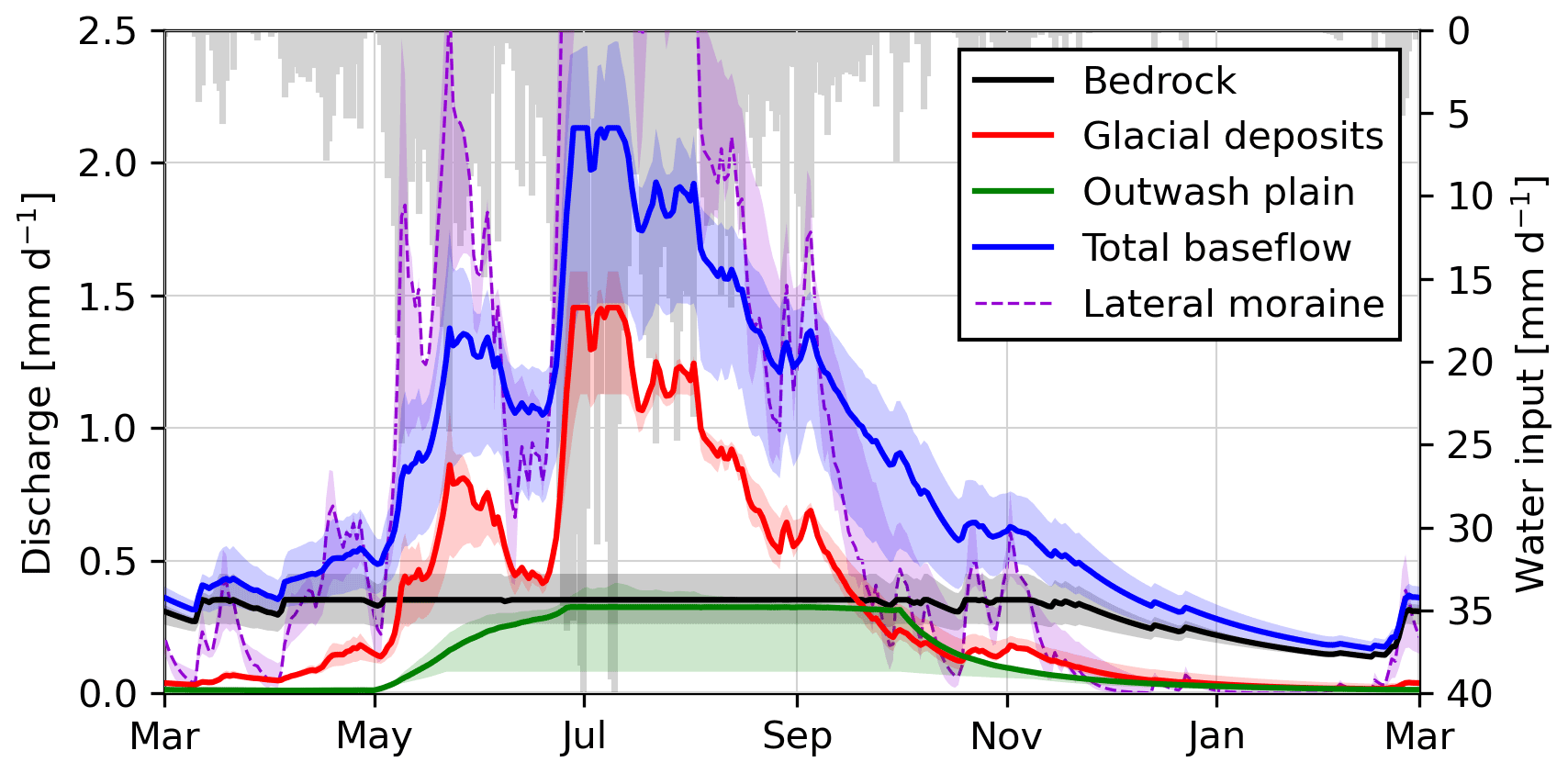
Figure 12 Evolution of modeled groundwater baseflow discharge of different hydrogeomorphological landforms. Total baseflow represents the sum of the outwash plain, flat glacial deposits, and bedrock discharge; steep lateral moraines are also plotted but are not considered in the sum of baseflow due to their fast response. Simulated total water input (snowmelt and rain) is plotted in grey.

The third hypothesis is that the storage occurs mainly in the bedrock and that sufficiently short flowpaths allow this storage to drain during the winter. This hypothesis is likely since large fractures may occur due to glacier debuttressing (Bovis, 1990; Grämiger et al., 2017) and groundwater seepage through deep fractures probably occurs underneath other landforms and cannot be measured directly. Moreover, some studies have reported similar catchment-scale storage in elevated catchments, although it is usually not clearly associated with a distinct hydrological unit. In particular, in a similar highly glaciated catchment, the work of Hood and Hayashi (2015) reported a peak catchment-scale storage in spring of 60 to 100 mm. Moreover, the work of Oestreicher et al. (2021) modeled an estimated catchment-scale storage change of 70 mm in a Swiss glaciated catchment of similar glacier coverage, which they could relate to a deep borehole water head change (Hugentobler et al., 2020). Such estimates represent the peak spring storage, accounting for all storage units, and not only the winter storage estimated in our study. Based on the rough estimates of Fig. 8, the peak summer storage estimated is 30 mm for flat glacial deposits and the outwash plain and 23 mm for the steep lateral moraines, which, combined with a bedrock storage of 40 mm, would result in similar numbers. Finally, during a cold spell in Otemma, some evidence of the contribution of deeper, older groundwater was observed as depicted by a fast increase in EC in wells C2 and D2 (Fig. 5), which could be due to older water exfiltrating from the bedrock.

Based on the above discussion, we suggest allocating the missing storage to bedrock storage with a maximum of 40 mm, which we can then add to our previous landform-based model (Eq. 12) with a recession constant ($\mathrm{1}/\mathit{\alpha }$) of 115 d to reflect the baseflow recession analysis. The resulting baseflow of each landform is shown in Fig. 12.

5.2 Landform hydrological connectivity

While our approach identifies the relative size and seasonal hydrological response of proglacial landforms, we use a simplistic recharge model. In reality, hydrological connectivity from the water sources and between landforms will ultimately drive the amount of actual recharge. Due to the coarse and barren nature of the sediments in such environments and the limited presence of soils, it can be expected that any water input will infiltrate into the sediments (Maier et al., 2021). It has also been shown that groundwater flow is driven by the bedrock topography underneath the landform, where a strong change in hydraulic conductivity drives the water downslope (Hayashi, 2020; Vincent et al., 2019). We can therefore assume that recharge occurs directly at the location of the water input, percolates until the bedrock and is then directed downslope. In the case of snowmelt, this recharge will gradually move upslope with the snow line during summer, a zone where talus slopes and bedrock are frequent. Water will rapidly be directed downslope at the bedrock interface and directed in zones of bedrock depression, concentrating the flow and thus providing little recharge to other downhill-sloping deposits. Water may also reach a flatter zone in hanging valleys, where flatter morainic material may be present in rock overdeepenings, which likely act as an immobile storage, where groundwater only overflows above the bedrock, similarly to a fill-and-spill mechanism (Tromp-Van Meerveld and McDonnell, 2006). The concentrated groundwater flow eventually reaches either the main stream or a flat glacial deposit (moraine or outwash plain) and acts as point recharge, so that only areas located below a zone of bedrock convergence will receive recharge. Similarly, glacier melt recharge will mostly occur along the reach of the glacial stream at the valley bottom and will maintain high groundwater storage in outwash plains or flat moraines exclusively.

5.3 A sound perceptual model for the hydrological functioning of a glaciated catchment

We summarize here the gained insights into a perceptual model (Fig. 13) of the hydrological functioning of the Otemma catchment, augmented with an additional “missing” storage which we tentatively allocate to bedrock (Sect. 5.1.5). In this representation, the partitioning between the different sources of water recharging each landform are taken from the results of our landform-based model of the Otemma catchment (Fig. 8). We also provide a comparison of the discharge amounts provided by each landform proportional to the results of Fig. 12.

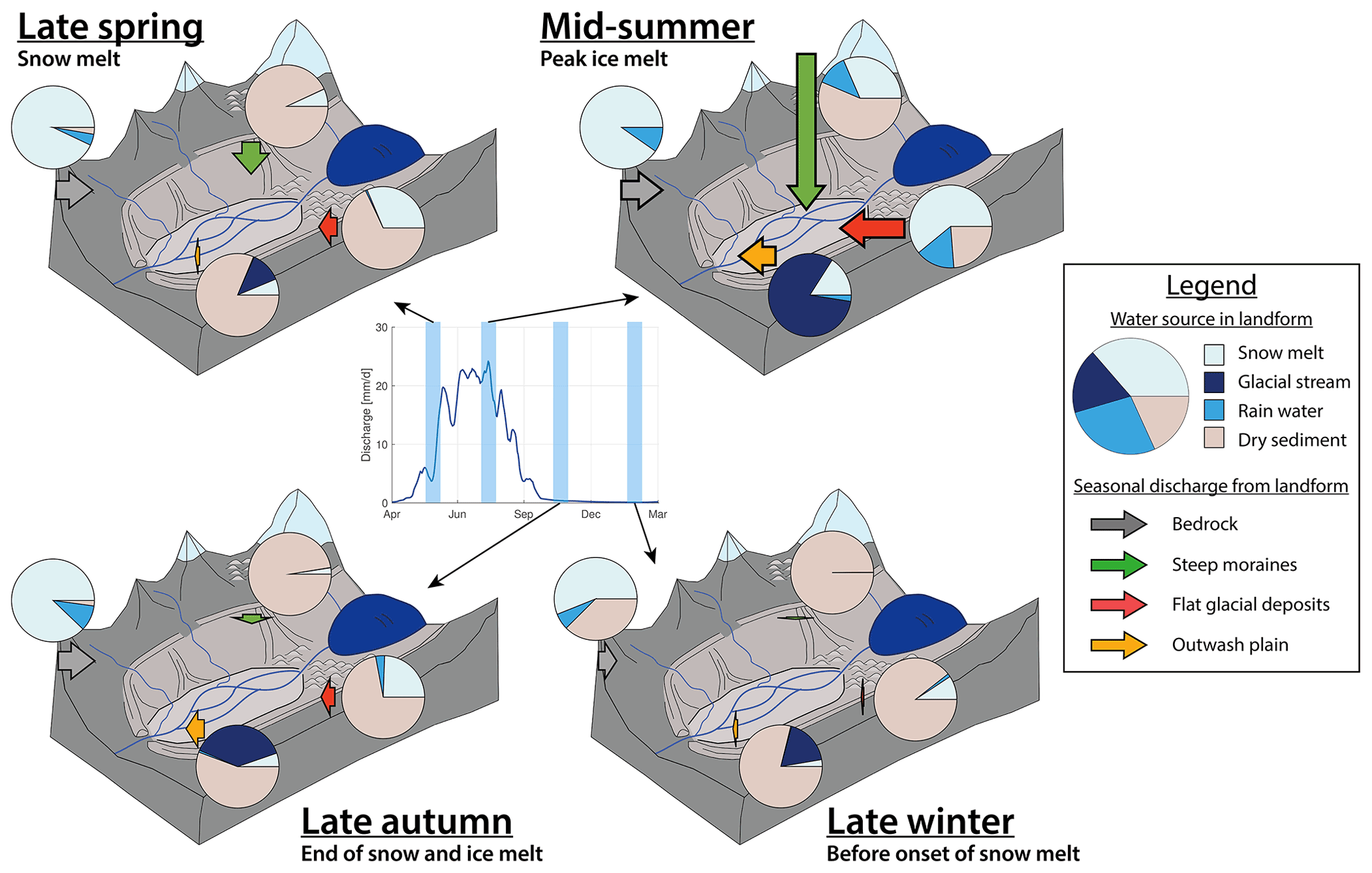
Figure 13 Perceptual model of groundwater dynamics in the Otemma catchment during four key hydrological periods. The central hydrograph represents the mean daily catchment-scale river discharge for the year 2015. The pie charts represent the seasonal partitioning of the three water sources (rainwater, snowmelt, glacial stream) calculated based on recharge and outflow (Sect. 3.5) for the three main superficial landforms as well as a bedrock aquifer. The source “Glacial stream” represents the mixed discharge leaving the glacier outlet and is an undefined mix of ice melt and snowmelt as well as of any liquid rain transiting through the glacier. The share of dry sediments represents the percentage of aquifer storage drained compared to the calculated maximum storage (Sect. 4.4), which is 40 mm for bedrock (missing storage), 23 mm for the steep lateral moraines, 19 mm for flatter glacial deposits, and 11 mm for the outwash plain. The length of the arrows represents the relative magnitude of the baseflow discharge estimated in Fig. 12 for each landform.

The perceptual model illustrates well how steep lateral moraines may provide large water amounts during peak snowmelt or strong rain events in mid-summer but drain very rapidly in fall. Talus slopes were not included in the perceptual model, as they play a marginal role in the Otemma catchment and have even faster drainage than steep moraines. In contrast to steep slopes, the baseflow provided by the bedrock aquifer appears more stable, although its storage decreases by half during winter. In a perspective of future early snowmelt, the model shows that most landforms may become dry much more quickly, with the exception of (i) the outwash plain, which receives water from the glacial stream, and (ii) the bedrock, which drains slowly, highlighting the future increasing importance of such aquifers for providing wetness and maintaining favorable ecological conditions.

In this representation we also neglected the impact of permafrost melt, although it is likely present at high elevation and in north-sloping moraines (Boeckli et al., 2012) and may provide some future additional meltwater in glaciated catchments, as shown in the work of Rogger et al. (2017). Rock glaciers were also not included as their presence is marginal currently in Otemma, but their role in storing and releasing water may become increasingly important since they have a capacity to store water on timescales of months, as shown in Table 2 and as discussed in more deglaciated catchments in Austria (Wagner et al., 2021).

6 Conclusions

This study attempted to bridge the gap between the catchment-scale response of a high-elevation glaciated catchment and the hydrological behavior of its landforms, using the case study of a large glacier in the Swiss Alps. The quantitative analyses are simple and are based on a rough estimation of the hydrogeological response of different landforms. Nevertheless, the analysis framework identified the order of magnitude and the timing of the contribution of the different landforms and is readily transposable to other case studies. The resulting perceptual model provides a realistic representation of the main drivers of the groundwater dynamics of the deglaciated zones of a typical glaciated catchment, which can serve as a blueprint for future experimental works as well as for hydrological model development. One clear uncertainty lies in the estimated hydraulic conductivities per landform, in particular their variability in space and depth. In addition, we had to attribute a large part of the groundwater storage to an unidentified compartment, which is likely partially due to a bedrock compartment but could also be due to a combination of meltwater and a subglacial compartment. Future research is needed to specify the very nature of this groundwater storage.

We have shown that superficial geomorphological landforms have a relatively limited capacity to store or release water at timescales longer than a few days, partly because of steep slopes but also due to the generally high hydraulic conductivity. In the future, two main changes can be expected. Firstly, with increasing glacier retreat, the extent of flatter landforms at the valley bottom will increase and may accumulate sufficient sediments to create new outwash plains or flat hummocky moraines that would increase the overall groundwater storage. It remains unclear how many sediments are produced with decreasing glacier volumes and whether they will be deposited or transported downstream (Lane et al., 2017; Carrivick and Heckmann, 2017). Secondly, with increasing vegetation growth, the formation of soils with enhanced organic matter content and finer soil texture are expected, which will promote water retention and modify the surface hydraulic conductivity (Hartmann et al., 2020). Recent studies on the evolution of morainic structures have shown that limited changes occurred on timescales smaller than a millennium, with a slight decrease in hydraulic conductivity (Maier et al., 2020, 2021). Thus, the impact of soil–vegetation development on the hydraulic conductivity and the rate of aquifer drainage is likely limited. Nonetheless, early soil development and biofilm growth may start to modify the water retention locally (Roncoroni et al., 2019), promoting more superficial soil moisture but limiting water infiltration and promoting surface runoffs, which will likely modify groundwater recharge. Finally, the ecological feedback of vegetation development on bank stabilization may also play a role in limiting sediment export and slow geomorphological changes (Miller and Lane, 2018), which may preserve the current geomorphological landforms.

The framework used to analyze the hydrological behavior of selected landforms based on groundwater levels and electric conductivity recordings is readily transferable at relatively low costs to other glaciated catchments. Our EC data underline a large variability between the landforms and spatially across the outwash plain, in addition to strong variations with changing groundwater heads. This observation shows that simple mixing models based on few observations of groundwater electrical conductivity in selected sources are likely not representative of the contribution of each landform and may provide very erroneous estimates of groundwater contribution.

More sophisticated tracer work could complement these analyses in the future. In particular, analysis of stable water isotopes could provide interesting insights into the relative share of subsurface recharge resulting from snow and rain over the season. The use of other geochemical tracers (Hindshaw et al., 2011; Gordon et al., 2015) or even noble gases (Schilling et al., 2021) could provide further insights into the potential contribution from deeper bedrock exfiltrations as well as better constrain the length or travel time of certain groundwater flowpaths.

Appendix A: Diffusion model analysis

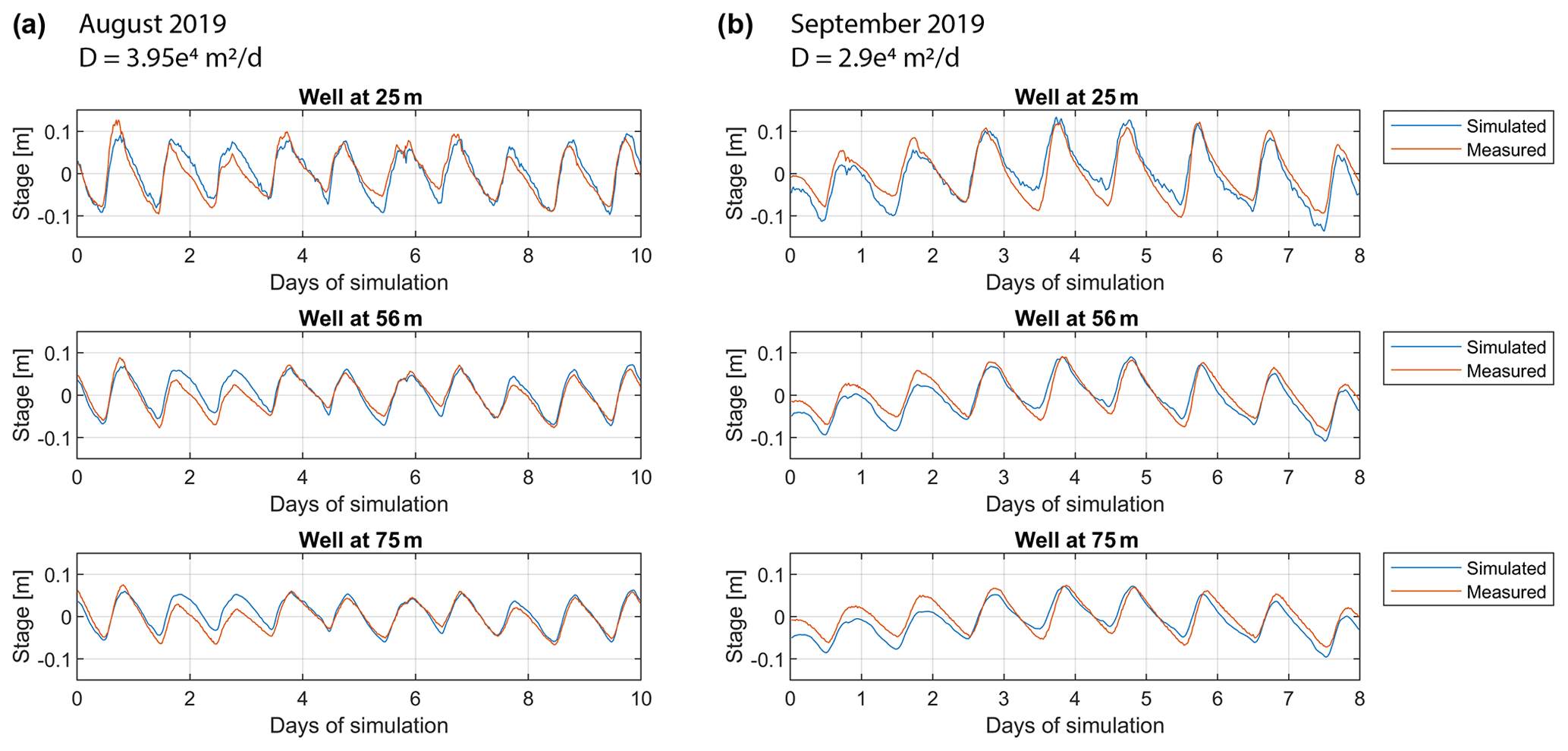
Figure A1 Measured and simulated water head variations for piezometers along the downstream transect “B” for the best calibration of the diffusion parameter D and for (a) the high-flow condition in August 2019 and (b) lower-flow condition in September 2019.

Figure A2 Measured and simulated water head variations for piezometers along the upstream transect “D” for the best calibration of the diffusion parameter D and for (a) the high-flow condition in August 2019 and (b) the lower-flow condition in September 2019.