the Creative Commons Attribution 4.0 License.
the Creative Commons Attribution 4.0 License.
 | 02 Dec 2022
Coastal topography and hydrogeology control critical groundwater gradients and potential beach surface instability during storm surges
Anner Paldor
Nina Stark
Matthew Florence
Britt Raubenheimer
Steve Elgar
Rachel Housego
Ryan S. Frederiks
Ocean surges pose a global threat for coastal stability. These hazardous events alter flow conditions and pore pressures in flooded beach areas during both inundation and subsequent retreat stages, which can mobilize beach material, potentially enhancing erosion significantly. In this study, the evolution of surge-induced pore-pressure gradients is studied through numerical hydrologic simulations of storm surges. The spatiotemporal variability of critically high gradients is analyzed in three dimensions. The analysis is based on a threshold value obtained for quicksand formation of beach materials under groundwater seepage. Simulations of surge events show that, during the run-up stage, head gradients can rise to the calculated critical level landward of the advancing inundation line. During the receding stage, critical gradients were simulated seaward of the retreating inundation line. These gradients reach maximum magnitudes just as sea level returns to pre-surge levels and are most accentuated beneath the still-water shoreline, where the model surface changes slope. The gradients vary along the shore owing to variable beach morphology, with the largest gradients seaward of intermediate-scale (1–3 m elevation) topographic elements (dunes) in the flood zone. These findings suggest that the common practices in monitoring and mitigating surge-induced failures and erosion, which typically focus on the flattest areas of beaches, might need to be revised to include other topographic features.
- Article
(3784 KB) - Full-text XML
- BibTeX
- EndNote


Groundwater seepage can destabilize land areas, especially at the interface between terrestrial and submerged systems (Iverson, 1995; Iverson and Major, 1986; Iverson and Reid, 1992; Schorghofer et al., 2004; Stegmann et al., 2011). Recent studies have examined the characteristics of pore-pressure behavior, the associated groundwater seepage, and its effect on the stability of geomaterials (soils, rocks, etc.), including field observations (Mory et al., 2007; Sous et al., 2016), physical experiments (Schorghofer et al., 2004; Sous et al., 2013), numerical simulations (Orange et al., 1994; Rozhko et al., 2007; Schorghofer et al., 2004), and analytical models (Sakai et al., 1992; Yeh and Mason, 2014). There are several examples of seepage-induced failure of the surface (i.e., the mobilization of the soil skeleton) from around the world, including Japan (Yeh and Mason, 2014), California (Orange et al., 2002), and France (Stegmann et al., 2011).
Soil liquefaction and quicksand occur when pore pressures in the geomaterial rise to a point where its effective stress drops to zero and the material is fluidized and thus acts as a liquid. The distinction between the two terms is related to the mechanism inducing the rise in pore pressures, with liquefaction referring to cases where external forces (e.g., earthquakes) are involved. Quicksand is used for cases where the pore pressures rise due to intrinsic changes in the groundwater regime. At the coast, ocean (waves, surge, tides, inundation) and terrestrial (groundwater heads, precipitation, and overland flows) processes concurrently contribute to changing pore pressures in beach and nearshore sediments and could thus induce failure of the surface. Ocean effects on pore pressures, groundwater flow, and seepage occur due to wind waves, storm surges, and tsunamis. For example, a one-dimensional analytical model suggests that, during a tsunami, vertical hydraulic gradients can destabilize sediments and increase the potential for sediment momentary liquefaction, consistent with laboratory experiments (Abdollahi and Mason, 2020; Yeh and Mason, 2014). Laboratory experiments (Sous et al., 2013) suggest that the magnitudes of hydraulic gradients in the beach due to infiltration from sea-swell and infragravity waves depend on the wave frequency, cross-shore position, water table overheight, and presence of standing waves. A large-scale (250 m) flume study of a barrier island showed that waves can alter the coastal groundwater head distribution significantly and can change cross-island and local (under the ocean beach) hydraulic gradient directions (Turner et al., 2016). Field observations of pore pressures over several tidal cycles in a microtidal beach (Sous et al., 2016) suggest breaking-wave-driven onshore increases in the water surface (setup) over the 10 m nearest the shoreline induced groundwater head changes of O (0.1 m) (Sous et al., 2016). Furthermore, density-driven flow at the subsurface transition zone between fresh terrestrial groundwater and saline groundwater can produce intense, localized seepage (Burnett et al., 2006). Rapid changes in seepage characteristics (locations, magnitudes, direction) during extreme events may lead to quicksand (i.e., loss of particle-to-particle contacts and sediment effective stresses) and sediment mobilization, resulting in erosion and structure destabilization.
Observations, theories, and simulations have shown that the pore-pressure changes owing to energetic ocean waves can reduce effective stresses and may cause failure of structures and surfaces (Chini and Stansby, 2012; Mory et al., 2007; Sakai et al., 1992; Sous et al., 2013; Yeh and Mason, 2014; Michallet et al., 2009). Measured pore-pressure changes in beach sediments during intense waves suggest that momentary liquefaction and quicksand may occur at shallow depths (<1 m) below the surface (Mory et al., 2007), consistent with theory (Sakai et al., 1992). Analytical solutions for the effective stress in an idealized seabed suggest that waves can alter the stresses in the upper meters of the seafloor significantly (Mei and Foda, 1981; Sakai et al., 1992). Simulations of a theoretical two-dimensional porous medium, where an increase in pore pressure is applied at the bottom of the layer from a point source, revealed that different spatial failure patterns (i.e., the geometry of the slip surface) can occur under various stress regimes (i.e., distribution of stresses in the soil) (Rozhko et al., 2007), although the process that leads to the simulated change in the pore-pressure distribution was unexplored.
Apart from waves, storm surges could also alter the onshore hydrogeological regime and potentially reduce the stability of the beach surface. Recently, Yang and Tsai (2020) modeled groundwater response to coastal flooding in the Greater New Orleans area and found that the interaction between flood water and surface water may destabilize levees in the area. This work focuses on the influence of alongshore topography and hydrogeological factors on geotechnical impacts near the shoreline owing to ocean surges driven by coastal storms, which are projected to intensify and become more frequent in the future (Chini and Stansby, 2012; Tebaldi et al., 2012). In particular, the three-dimensional dynamics of surge-induced flooding and the resulting shore-parallel distribution of pore-pressure gradients in sandy beach areas are not well understood. Specific questions addressed in this work are the following. (1) Can surge-induced pore-pressure changes promote sediment quicksand of the uppermost sediment layers (<5 m), and which areas across the beach are the most vulnerable? (2) What is the relationship between beach morphology and the spatiotemporal evolution of pore-pressure gradients? (3) How do the hydrogeological properties (hydraulic conductivity, groundwater recharge) of the coastal system affect the potential for failure? A conceptual model is presented for the effect of storm surges on coastal groundwater heads (Sect. 2), a criterion is derived (Sect. 3) for quicksand for beach slopes with groundwater discharge based on existing solutions (Briaud, 2013), and a model framework is described (Sect. 4) and used to simulate surges in theoretical beach settings and to examine their effect on sediment stability (Sect. 5).
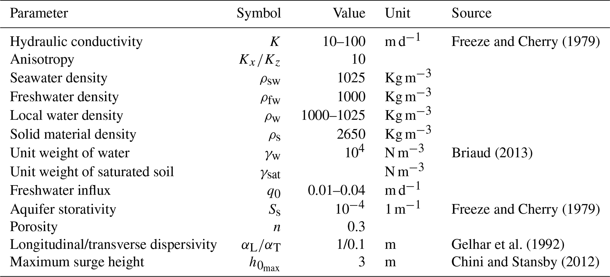
A conceptual model of a coastal system (Fig. 1) includes infiltration of rain that recharges the aquifer with freshwater, resulting in fresh groundwater flow toward the ocean. In the nearshore area (typically within meters of the shoreline), an inclined freshwater–saltwater transition zone develops between the saline groundwater underlying the seafloor and the terrestrial fresh groundwater. The density gradient at the transition zone deflects the fresh groundwater flow upward and produces focused groundwater discharge near the coastline that can be amplified by an order of magnitude or more relative to the average flow rate in the aquifer (Paldor et al., 2020). In phreatic aquifers, submarine groundwater discharge typically occurs within tens of meters of the coastline, depending on the recharge rates and aquifer properties (Bratton, 2010). In systems where the discharge is into a body of freshwater (e.g., a lake), the bottom of the lake is a constant head boundary, and thus the seepage is, by definition, perpendicular to the lake bed. This assumption is widely adopted in geotechnical calculations of groundwater discharge magnitudes. For example, in flow net solutions for classic dam and levee problems, the bottom of the river on both sides of the dam or levee is considered an equipotential line (Briaud, 2013). However, along the bottom of a saltwater body, the freshwater-equivalent head is variable with bathymetry, and hence the seepage is not necessarily perpendicular to the seafloor and possibly represents a complex, three-dimensional problem with high spatiotemporal variability. To assess the risk of quicksand in the context of the freshwater–saltwater transition zone and during coastal flooding events, the vertical component of the hydraulic gradient is computed to evaluate the potential for quicksand (as will be derived in the following section) with the application of the variable-head boundary condition and the inclusion of variable-density flow solutions. It should be highlighted that, in the current work, no effects of long-term loading and residual liquefaction were investigated. Hereinafter, the vertical hydraulic gradients will be discussed rather than the pore pressures or heads. In the next section the equations for soil failure potential in terms of the head gradients are derived based on previous derivations (Briaud, 2013). The magnitude of the hydraulic head gradient, which according to Darcy's law is the magnitude of the seepage vector divided by the hydraulic conductivity, is denoted i (Fig. 1). The seepage vector is the specific discharge, which is computed as the outflow vector at top nodes of the domain. In two dimensions, this vector has two components – horizontal (−Kix in Fig. 1) and vertical (−Kiz). This work focuses on the vertical component. Other variables used in the following calculations are shown in Fig. 1 and summarized in Table 1.
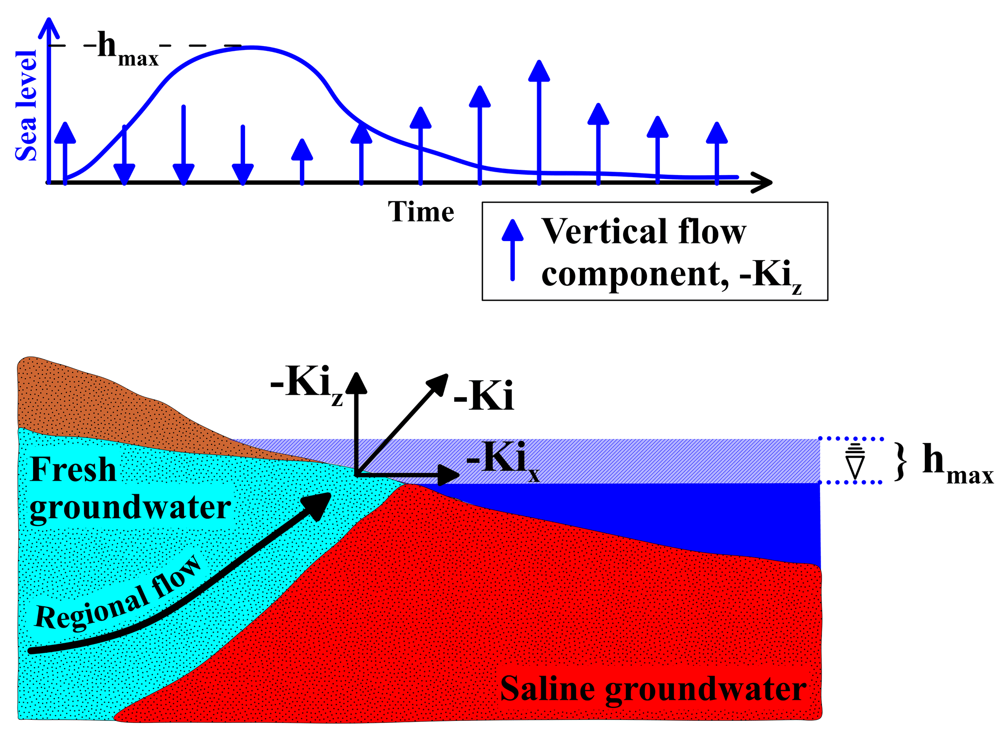
Figure 1A hypothetical coastal hydrogeological system. Regional fresh (light blue) groundwater flows to the sea and upward due to variable-density flow along the freshwater–saltwater (red) interface. In the nearshore area, focused groundwater discharge occurs either into the sea (blue) or along a seepage face onshore. As shown at the top of the figure, when the surge begins, the direction of flow reverses (infiltration), and when the sea level reaches its maximal level (hmax), the surge retreats and the direction reverts back (exfiltration). The upward (positive vertical component) flow reaches a maximum when the sea level is back to the pre-surge level, before decaying to the steady-state magnitude.
Table 1Variables used in the theoretical calculations and numerical simulations.
2.1 The criterion for quicksand under groundwater seepage
Two terms that are often confused are “liquefaction” and “quicksand”, with the former being used for earthquake-induced fluidization of the soil and the latter being related to failure due to upward flow (Briaud, 2013). The physical meaning of the two is similar – geomaterial becoming suspended in a colloidal solution, which can result in erosion and sediment mobilization, or loss of support of any infrastructure built into the soil. Here, the term “quicksand” is used, as the analysis refers to surge-induced changes in the subsurface flow rather than seismically induced flows. Following Briaud (2013), quicksand occurs when the pore pressure (uw) at a certain depth (z) exceeds the total stress (σ), i.e., when the effective stress (σ′) goes to zero:
Neglecting the possibility that gas is still trapped in the pores and assuming a submerged unit weight can be applied, the criterion for localized quicksand in inundated regions can be written in a gradient form (Goren et al., 2013) in which the vertical pore-pressure gradient (positive downward gradient generates upwards flow) exceeds the submerged unit weight of the soil (γsub):
where
in which ρs is the density of the beach material (sand), and ρw is the density of the local water, which has a value between that of seawater (ρsw≈1025 kg m−3) and freshwater (ρfw≈1000 kg m−3). This failure criterion is similar to Yeh and Mason (2014), who studied liquefaction of a fully saturated sediment following a tsunami.
The constant value of porosity (n=0.3) is typical for sandy soils but neglects localized variations in sand bulk density in the simulated topography. The use of γsub as the representative unit weight of simulated soil is appropriate for soils that are fully submerged, as it accounts for the buoyancy effect, considering the unit weight of the overlying water column (γw). However, for the parts of the model landward of the inundation line, the saturated unit weight may be more suitable. This means that adopting γsub uniformly may be an underestimate of the actual unit weight in real systems (). Nevertheless, we used γsub since the aim of this work is to harness a hydrologic modeling framework to assess the spatiotemporal distribution of surge-induced changes in hydraulic gradients. To that end, the quicksand assessment is limited to the effects of vertical pressure gradients and the application of the submerged unit weight. It should be noted that studies have shown that partially saturated sediments (e.g., in inundation areas) are typically prone to momentary liquefaction (Mory et al., 2007; Yeh and Mason, 2014). Mory et al. (2007) showed that even a 6 % air content may increase the potential for momentary liquefaction. For the gradient-form criterion to hold, this condition would need to be met continuously from the surface to the depth of the liquefied layer (Goren et al., 2013), as accounted for in the analysis below.
Here, the quicksand criterion is related to vertical components of seepage vectors to compare the results of the groundwater model with the failure criterion. The three-dimensional model considered here (see below) could be used to examine the horizontal components too and to analyze the potential for shear failure, not only for quicksand and momentary liquefaction (Zen et al., 1998). However, for the sake of simplicity and in the interest of focusing on the questions addressed here, such an expansion is not attempted in the current study. It would require further assumptions about the soil characteristics (internal friction, cohesion) and a localized analysis of the local slopes for each point in the domain. According to Darcy's law the vertical specific discharge (denoted vz with dimensions MT−1) is equal to the product of the (local) vertical head gradient and the vertical hydraulic conductivity Kz:
Thus, the vertical pressure gradient becomes
Substituting Eqs. (3) and (5) into Eq. (2) yields
From Eq. (6), the value of the critical vertical head gradient (ic) is that above which the effective stress is zero or less:
This result is similar to that derived by Briaud (2013) for a general case of quicksand. Here it is derived specifically to facilitate direct calculations of surge-induced changes in the groundwater flow regime as output by the hydrologic model. Using Darcy's law in this context assumes that during the surge the groundwater flow remains largely laminar, which is likely for storm-surge conditions and is a common assumption in similar studies (Abdollahi and Mason, 2020; Guimond and Michael, 2021; Paldor and Michael, 2021; Paldor et al., 2022; Yang et al., 2013; Yu et al., 2016). For convenience, the magnitude of downward (negative) vertical head gradients which initiate upward (positive) vertical velocities and therefore potentially destabilize the soil is hereinafter denoted iz and presented in positive values. Using typical values for porosity, solid particle density, and freshwater density for beach material ( kg m−3; ρfw=1000 kg m−3, respectively), Eq. (7) suggests that the critical value of the vertical head gradient is about ic=0.15. While the parameters can have ranges of values for given systems, the following analyses use this value as a threshold for quicksand, with simulated values of iz normalized by the critical value ic=0.15 as the seepage–liquefaction factor (SLF):
We term the criterion the “seepage–liquefaction factor”, while it is noted again that the actual failure mechanism discussed here is quicksand, as it is not related to seismic loading. In Eq. (8), iz is the actual simulated or observed vertical head gradient, defined as (Eq. 4), and ic is the theoretical quicksand threshold (Eq. 7). Thus, any point in space and time in which simulated SLF is close to 1 is potentially nearing quicksand. A layer in which SLF approaches 1 continuously from the surface to a depth Zl is considered a “critical layer” of thickness Zl. The SLF defined here is the reciprocal of the factor of safety defined by Yang and Tsai (2020) for levees under storm-induced groundwater seepage, and thus it should be noted that in the analysis presented here lower values of SLF represent greater stability.
The effect of storm surges on groundwater flow is simulated using Hydrogeosphere (HGS) – a three-dimensional numerical code that couples surface and subsurface flow and solute transport (Therrien et al., 2010). For the surface flow, HGS solves the Saint-Venant equations (also known as nonlinear shallow water equations), and for the variably saturated subsurface flow, it solves the Richards equation. The salt transport equation is solved in its advective–dispersive form, and the variable-density flow solution is coupled to the transport solution through a linear equation of state. Hydrogeosphere has been successfully employed to simulate storm surges in several recent studies (Guimond and Michael, 2020; Yang et al., 2013, 2018; Yu et al., 2016), and here it is applied to assess the risk of quicksand and erosion from surge-induced porewater head gradients. This interdisciplinary approach, using a groundwater model in the context of coastal geomechanics, has recently been applied by Yang and Tsai (2020) to assess the impacts of floods on the groundwater regime in the Greater New Orleans area and its implications for the factor of safety of levees. Several other studies have applied different methods to relate between changes in the groundwater regime and the stability of the surface (Chini and Stansby, 2012; Sakai et al., 1992; Sous et al., 2013; Yeh and Mason, 2014). The novelty in this study relates to the harnessing of a three-dimensional integrated hydrologic model in a generalized form to explore the mechanisms that dominate surge-induced quicksand formation. Applying the fully coupled model to different generalized topographies (detailed below) allows us to study the alongshore distribution of critical gradients, which is commonly overlooked in similar studies (Yeh and Mason, 2014).
The model domain (Fig. 2) is 4000 m (cross-shore, X) by 2500 m (alongshore, Y), extending to a depth of 30 m below the mean sea level (Z=0). The terrestrial extent of the domain is 3550 m (450<X≤4000), with the ocean spanning (Fig. 2). The elevation at the ocean side boundary is , so the seafloor slope is . This slope is representative of US Atlantic and Gulf coastal systems averaged over large cross-shore distances (e.g., from the beach to the mid-continental shelf). Although local slopes in the surf and beach are often much steeper than those used here, this study is focused on the quicksand potential in and near the inundated dune system. The average surface elevation inland (X=4000 m) is 5 m, so that the average land surface slope is . Thus, there is a change in average slope at the coastline, as the offshore portion is steeper (∼0.0022) than the onshore portion (0.0014), as in many coastal areas. To justify this setting, we ran a simulation with a −0.5 m sea level (i.e., still-water shoreline at X=225 m), which indicated that critical vertical hydraulic gradients occur near this change in overall slope irrespective of the shoreline location (Fig. A1 in the Appendices). A simulation with a larger beach slope (; slope = ) resulted in similar vertical hydraulic gradients to the baseline slope (0.0022) (Fig. A2 in the Appendices), indicating that, although the baseline slope is lower than is typical, the analysis based on it is also valid for steeper slopes. The domain of the finite-difference model consists of 44 000 rectangular cells, where the cell sizes in the X and Y directions are 25 and 50 m, respectively. The cell size in the Z direction varies from 8 m at the bottom of the domain to about 0.5 m in the top 2 m to balance between computation time and the resolution necessary to resolve the dynamics close to the surface (Fig. 2). The homogenous hydraulic conductivity Kx is 50 m d−1 for the baseline simulation, and values of Kx = 10, 25, and 100 m d−1 were also simulated as part of a sensitivity analysis. In all the simulations, the anisotropy was 10 (i.e., the vertical hydraulic conductivity, Kz, was 10 times lower than the horizontal hydraulic conductivity, Kx). This range of hydraulic conductivity with a porosity, n, of 0.3 is typical for sandy beach environments (Freeze and Cherry, 1979). Anisotropy of porous material may represent the presence of horizontally extended low-K lenses (e.g., localized compacted clay lenses), which reduce the conductivity in the vertical dimension preferentially. Although a change in K could be associated with a change in n for some sediments and mixtures, due to the potentially complex relationships between porosity and the sediment textural properties, including grain size distributions, shapes, and K, the porosity was kept constant in the simulations presented here.
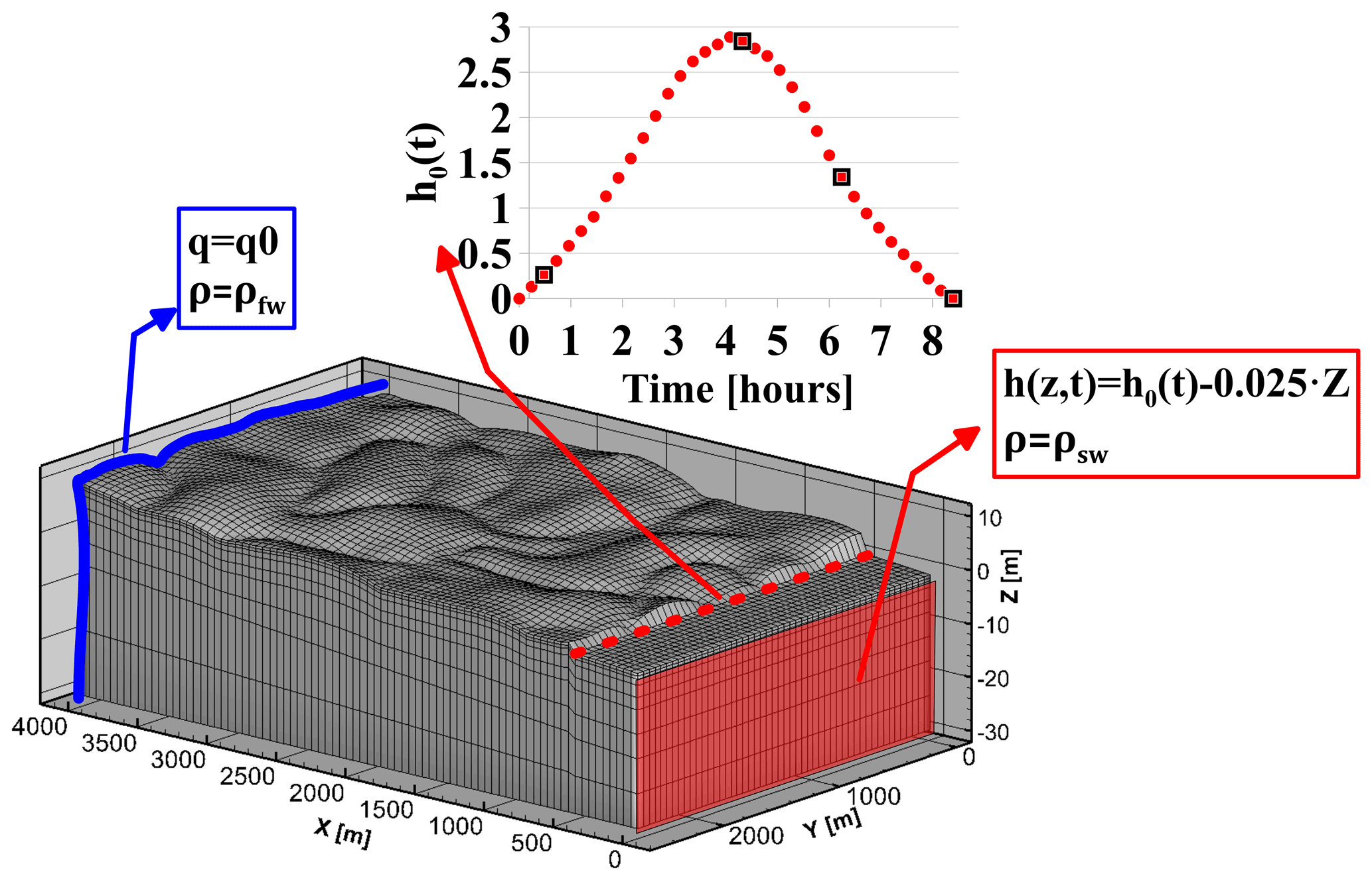
Figure 2Hydrogeosphere model domain as a function of the vertical Z, cross-shore X, and alongshore Y dimensions, boundary conditions (red and blue boxes), and the surge height evolution curve (inset). The blue curve is the terrestrial freshwater recharge boundary, the red rectangle is where a fixed seawater head and concentration are applied to the subsurface domain, and the red dashed line is where the sea level height boundary condition (h0(t)) is applied to the surface domain. For the steady-state simulations h0(t)=0 and for the transient simulations, the curve in the inset is applied. The black squares in the inset mark the times plotted in Fig. 4.
The boundary conditions in the simulations were applied in two stages – a steady-state period and a transient surge period. For the steady-state simulations, terrestrial boundary conditions of constant freshwater-specific recharge (q=q0, ρ=ρfw) were applied to the vertical wall at the inland edge of the subsurface domain at X=4000 (blue curve in Fig. 2) (Ataie-Ashtiani et al., 2013; Yang et al., 2018; Yu et al., 2016). The opposite edge of the domain at X=0 (red wall in Fig. 2) was a typical sea boundary condition with depth-dependent head and saline ocean water (; ρ=ρsw). On the surface domain the only boundary condition is applied to the coastline (X=450 m, red dashed line in Fig. 2) as a fixed, time-dependent head (h=h0(t)) and seawater density (ρ=ρsw). The applied head on the coastline was held at zero through the steady-state simulations. For the transient surge simulations, the coastline head was varied over 8.5 h between zero and a 3 m maximum surge height (inset in Fig. 2). A sea level of 3 m above the mean represents a combined high-tide and surge event with a projected return period of 100 years by the year 2050 on the East Coast of the United States (Tebaldi et al., 2012). The ocean surface was assumed to be spatially constant at any time, and effects of wind waves were not simulated. The simulated surge height is comparable in magnitude to macro-tides, but the differences in frequency (macro-tides are diurnal) mean that macro-tidal beaches are likely in equilibrium with respect to sediment mobility, which is not the case for storm surges.
The sensitivity of the results to the topography and hydrogeologic parameters was tested, including freshwater influx (0.01<q0<0.04 m d−1, Fig. 2 and Table 1) and hydraulic conductivity (10<Kx<100 m d−1, Table 1, typical values for sandy beaches, Freeze and Cherry, 1979). For the baseline hydraulic conductivity (Kx=50 m d−1), the range of overall (land-to-sea) hydraulic gradients, calculated as , was 0.0002 and 0.0008, on the lower side of typical coastal settings (roughly around 0.0010), and so the calculated hydraulic gradients in the current analysis are considered a conservative estimate. Two topographies (Fig. 3) (Yu et al., 2016) were generated with ARCMAP 10.0 Geographic Information System (GIS) software (ESRI, 2011), using multi-Gaussian random fields that were transformed (Zinn and Harvey, 2003) to connect either topographic highs or lows rather than the median topographic values as in the non-transformed multi-Gaussian fields. The first topography, named “River” (Fig. 3a), is characterized by surface depressions that connect to the sea. The topographic lows are connected, forming “river”-like patterns in the surface morphology superimposed on the background slope of 0.0014. The second topography, “Crater” (Fig. 3b), features connected crests surrounding disconnected surface depressions, such that the highs are connected, forming “crater”-like shapes. The two topographies do not mirror each other (Fig. 3) but represent reverse alongshore trends near the shoreline (450<X<500 m) in which the area around 0<Y<300 m (2200<Y<2500 m) is the highest (lowest) for the River topography and lowest (highest) for the Crater topography. Comparisons with real topographies of the Delaware coastal plains (Yu et al., 2016) suggested that the River topography best represents meso-topography in that area. However, the Crater topography provides important insights into how meso-topography controls the evolution of head gradients during storm surges even though they are not necessarily representative of real systems. It is noted that exploring four values of hydraulic conductivity and two types of synthetic topographies may be a limited representation of natural systems. For example, Yu et al. (2016) showed that topographic connectivity is a dominant factor in the vulnerability of coastal aquifers to storm surge salinization, and we consider here only two of the topographies simulated there. However, the tested topographies and conductivities in this work serve as a preliminary exploration of hypothetical conditions that are likely representative of many natural systems, but this is certainly not inclusive. In extreme flooding events (e.g., tsunami), large-scale changes in surface morphology (e.g., landslides) may alter the pore-pressure distribution. These effects were excluded from the current work, as the simulated surface was considered constant throughout the simulation. Additionally, soil deformation and the resultant stress re-distribution were not considered in this model, as the hydrologic model (HGS) assumes constant porosity.
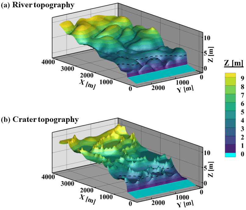
Figure 3(a) River and (b) Crater topographies as a function of the vertical Z, cross-shore X, and alongshore Y coordinates. Light blue is the offshore bathymetry, and the coastline is at X=450 m. The overall slope accounting for macro-topography is the same for both topographies, and the average elevation at X=4000 m is ∼5 m, making it a slope of . The dashed black curve marks the Z=3 m contour, which is equal to the maximum surge-induced sea level (hmax).
For each simulation, the vertical hydraulic gradients (iz in Eq. 8) are calculated for the modeled domain and normalized by the threshold defined by Eq. (7) (ic) to calculate the SLF (Eq. 8). As explained in Sect. 3 above, values of SLF that approach 1 are considered critical for quicksand. When SLF ≪ 1, the simulated surface theoretically is stable. Only upward, destabilizing velocities (exfiltration) are considered, and so negative velocities were assigned a value of iz=0.
The baseline case (“River” topography with q0=0.02 m d−1; Kz=5 m d−1) includes a 3 m surge and simulates the resultant changes in head gradients (Fig. 4). During the flooding stage when sea level is increasing, the head gradients increase landward in front of the moving surge, and in the flooded zone there is infiltration (head decreases downward, ∇h>0). After the peak of the inundation, when the high-water levels begin to recede, downward gradients (i.e., head increases downward, potentially destabilizing) develop underneath the still-water shoreline (X=450 m). These downward gradients increase in magnitude as the water level recedes, and the subsurface system relaxes back to background levels (not shown in Fig. 4) within ∼50 d for the high-K aquifers to ∼500 d for the low-K aquifers, in agreement with prior simulations of storm impacts (Robinson et al., 2014). The peak alongshore variation of the vertical hydraulic gradients occurs at the end of the flooding (t=8.4 h, Fig. 4d). The vertical hydraulic gradients onshore of the flooding front during run-up (Fig. 4b) develop in subaerial areas. As explained in Sect. 3.1 above, the calculated SLF for these zones should be based on the saturated unit weight () of sediments rather than the submerged unit weight (γsub, Eq. 3), and the model-predicted quicksand may not occur in real systems because saturated soils are more stable than submerged ones (Briaud, 2013).
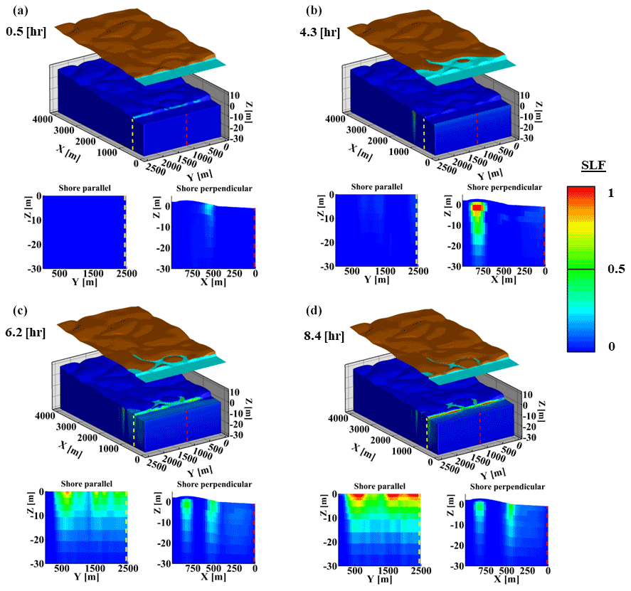
Figure 4Surface flooding and vertical hydraulic gradients at (a) 0.5, (b) 4.3, (c) 6.2, and (d) 8.4 h after the simulated surge begins. In each panel, the surface domain is shown on top, the subsurface three-dimensional domain and vertical gradients are shown below, and the two cross sections through the subsurface are shown: shore-parallel (left in each panel) and shore-perpendicular (right). The locations of the sections are shown on the three-dimensional plot as red dashed lines (for shore-perpendicular) and yellow dashed lines (for shore-parallel). Panels (a, b) are during the run-up stage and panels (c, d) are during the retreat stage. Refer to Fig. 2 for the surge height at each time shown here. Note that downward gradients (head increases downward) are plotted as positive values of SLF and upward gradients (head increases upward) are plotted as zero SLF.
The head changes (Δh in Fig. 5) between the steady state and the peak of the flooding inversely follow the topography (black contours in Fig. 5a and b). For the highest topographic elements (Y=0 m for “River” and Y=2500 m for “Crater”), which are not inundated, the simulated heads are approximately equal to the maximum ocean level at the dune crest (X∼460 m) and decay inland over ∼100 m. The maximum head changes (purple colors in Fig. 5a) inland of the shoreline (X>475 m) at peak surge occur in the inundated topographic lows. Toward the end of the simulated surge (t=7.2 h, Fig. 5b), the surge-induced increased pressures are released in the topographic lows (low values of Δh in Fig. 5b). The temporal differences in head between surge and calm conditions are also low in the topographic highs because the heads there did not rise significantly during flooding. In contrast, the intermediate topographic features show high head differences (dark purple in Fig. 5b). The lowest near-shore ( m, m) topography undergoes similar head changes during the peak surge for high and low K (compare Fig. 5a1 with Fig. 5a3). However, in the low K case (Fig. 5a3, b3), the heads are not released effectively as the surge recedes, and significant increased heads of ∼1 m difference remain near the end of the surge (compare Fig. 5b3 with Fig. 5b1 for X∼450 m).
When the surge has retreated (t=8.4 h), the head gradients at the dune toe (initial shoreline) (X=450 m) reach their maximum (Fig. 5c1–c3). In all the simulations, critical gradients (SLF → 1, red zones in Fig. 5c1–c3) are simulated at some locations below the shoreline, supporting the findings of several recent field studies in which quicksand was observed in response to inundation events (Sous et al., 2016; Yeh and Mason, 2014). The alongshore distribution of the surge-induced gradients is insensitive to the freshwater influx (q0), even though the antecedent local hydraulic gradients differed by up to a factor of 4 between simulations (Fig. A3 in the Appendix; note that the values of the antecedent local gradients are about an order of magnitude lower than the peak gradients). The depth and alongshore locations of the areas prone to quicksand (i.e., SLF ∼ 1) are sensitive to the topography (compare Fig. 5a1, b1, c1 with a2, b2, and c2) and the hydraulic conductivity (compare Fig. 5a1, b1, c1 with a3, b3, and c3). The two topographies exhibit a similar spatial pattern of SLF (Fig. 5c1 and c2) even though the differences in topography (Fig. 3) cause significant differences in the surge-induced head changes (Fig. 5a1 and a2). For example, the area to the left of the domain ( m) is a topographic low in the Crater topography and undergoes significant head changes at the peak of the flooding (Fig. 5a2), whereas for the River topography there is a topographic high for 300 m, which is not as strongly affected by the surge (Fig. 5a1). However, in both cases this area is where the least significant vertical head gradients develop (Fig. 5c1 and c2). This means that a monotonic relationship cannot be assumed between topography and vulnerability (i.e., the lowest/highest areas along the beach are not necessarily the most/least vulnerable).
The hydraulic conductivity has a significant effect on the simulated surge-induced gradients (Fig. A4 in the Appendix). Decreased hydraulic conductivity causes higher peak vertical gradients and changes the spatial (shore-parallel) distribution of the gradients (compare Fig. 5c3 with c1, especially near Y=1000 m, and also see Fig. A4). Furthermore, decreasing hydraulic conductivity alters the depth Zl of “critical layers” with SLF = 1 (Eq. 8) (compare Fig. 5c3 with c1). In the high-K simulations (Fig. 5c1 and c2), the depth Zl of these “critical layers” with SLF ∼ 1 ranges between 0 and 2.5 m, and in the low-K simulation (Fig. 5c3) Zl is up to ∼5 m.
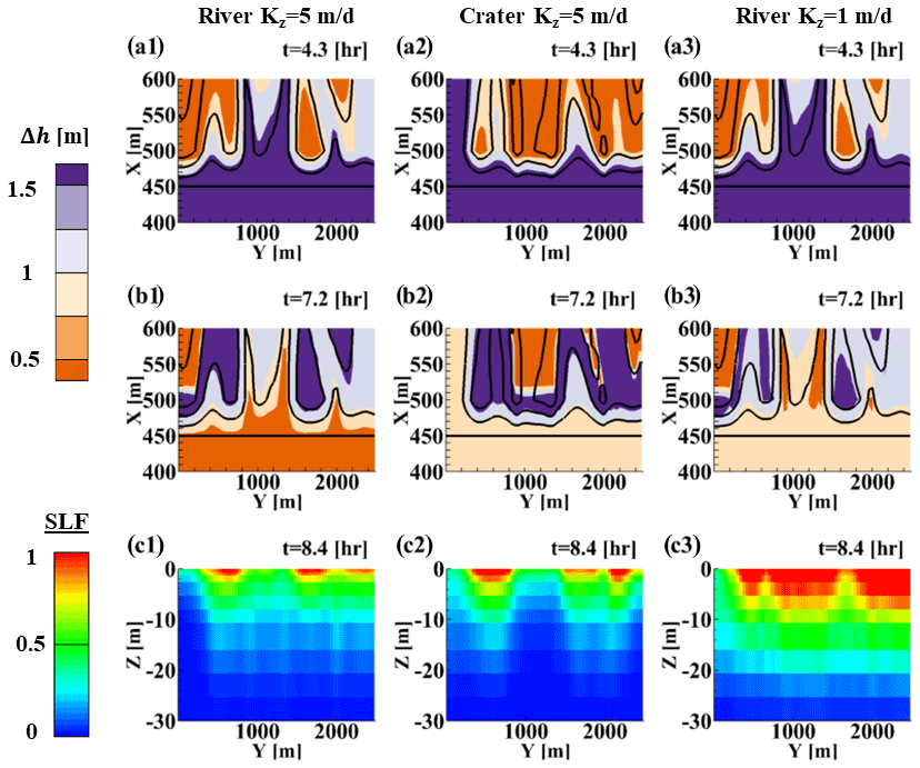
Figure 5Top row (a1–a3) maps of the maximum near-surface head differences between those at the peak of the flooding and the initial, pre-surge values (denoted Δh1) as a function of the cross-shore X and alongshore Y coordinates. Middle (b1–b3) maps of the maximum subsurface head differences between those near the end of the surge (t=7.2 h, Fig. 2) and the initial, pre-surge heads (denoted Δh2) as a function of X and Y. Bottom (c1–c3) quicksand potential SLF at the shoreline, X=450 m, as a function of the vertical Z and alongshore Y coordinates. These three metrics are plotted for the River topography with Kz=5 m d−1 (left, a1–a3), Crater topography with Kz=5 m d−1 (center, a2–c2), and River topography with Kz=1 m d−1 (right, a3–c3). In the upper and middle panels (map views a1–a3 and b1–b3) the black contours are surface elevations with 1 m intervals. The horizontal line at X=450 is the coastline (Z=0). The lower panels are plotted for t=8.4 h, the time at which the vertical gradients peaked in all simulations all along the coastline.
The relationship between coastal topography and the surge-induced quicksand potential is evident when comparing the surface elevations 50 m landward of the coastline (X=500 m) and the peak vertical gradients below the coastline for different topographies and Ks (Fig. 6). Here, the SLF = 0.7 contour is used because for engineering applications it is required to design structures with a buffer to ensure a satisfactory factor of safety. Furthermore, using the SLF = 0.7 provides better statistical stability since there are more locations with SLF ≥ 0.7 than with SLF = 1. For both topographies, when K is high, SLF typically remains less than 0.7 (in Fig. 6 where the blue diamonds = 0) at the shoreline adjacent to the highest (Z>3 m) and lowest (Z<1 m) topographic elements (marked by gray rectangles in Fig. 6a and b), suggesting that the intermediate topographic features may lead to the strongest vertical hydraulic gradients and quicksand potential. However, the height of intermediate features that produce high gradients may be dependent on the site and hydrogeological parameters. For example, in the two simulations with higher Kz, 1–3 m topographic features are associated with most of the significant surge-induced gradients (Fig. 6a and b). For the lower Kz case, significant gradients also occur below the lowest area (Fig. 6c), and only the highest area that is not inundated does not develop significant gradients (gray rectangle in Fig. 6c).
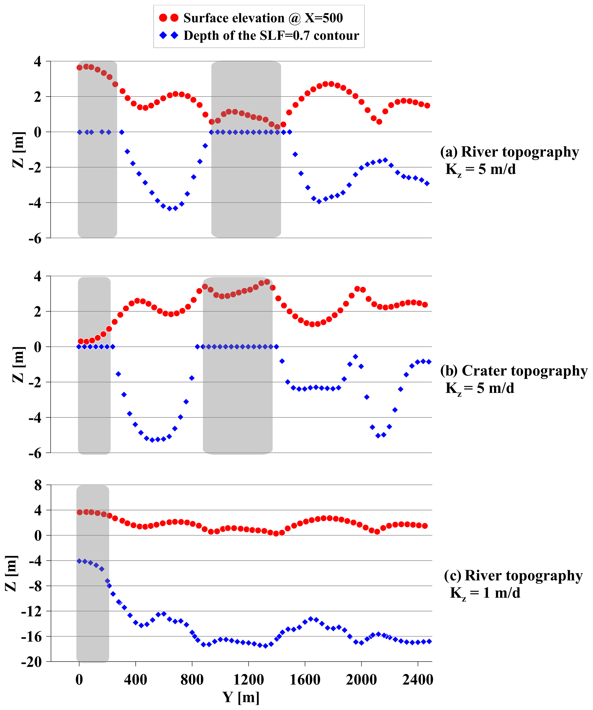
Figure 6Topographic elevation at X=500 m (50 m onshore of the shoreline, red circles) and depth of the SLF = 0.7 contour below the shoreline (blue diamonds) versus the alongshore coordinate Y for (a) the River topography with Kz=5 m d−1, (b) Crater topography with Kz=5 m d−1, and (c) River topography with Kz=1 m d−1. Deeper locations of the SLF = 0.7 contour (blue diamonds) mean thicker “critical layers”. The places where no significant critical layer develops (i.e., the elevation of the SLF = 0.7 contour is Z=0) are marked by gray rectangles.
5.1 Alongshore variability
The simulations suggest that alongshore variability of the magnitudes of the vertical gradients is strongly associated with the coastal topography (Figs. 4–6). To induce high gradients and deep critical layers when surge-induced increased heads are released, it is necessary to have flooding resulting in high infiltration and increased heads. Thus, topographic highs that are not inundated cannot develop high gradients (Figs. 5 and 6). Meanwhile, increased pressures are often released efficiently from inundated areas as the surge recedes. Topographic elements that are low enough to be inundated but that are also high enough to limit the post-surge exfiltration may prevent release of pressures with a thicker porous medium that impedes flow, possibly explaining the link between quicksand potential and intermediate topographic features (1–3 m high for a 3 m surge). This explanation would suggest that the characteristic elevation of “intermediate features” would scale with the surge magnitude. Pressure releases can also be limited by low hydraulic conductivity. Thus, the simulations suggest that the areas most susceptible to destabilization (i.e., deep critical layers) are those where topography is low enough to be inundated widely and high enough that the pressure release is limited. An important factor that likely plays a role in this relationship between intermediate topography and critical gradients is the horizontal gradient. In places where horizontal hydraulic gradients can develop, a more efficient dissipation of surge-induced pressures may be expected, and therefore critical gradients are less likely. This may explain the absence of critical hydraulic gradients from the steepest areas in the model, since these areas develop horizontal gradients. Horizontal gradients are also important when considering other modes of surface instability, such as shear failure. To assess the potential for shear failure, a Coulomb criterion must be derived, which is beyond the scope of the current study. Another factor that is known to control the vulnerability to storm-induced instability is the antecedent groundwater level which controls the infiltration capacity of flood waters (Cardenas et al., 2015). This may explain the absence of critical hydraulic gradients from the flatter areas of the model, leaving an intermediate range of topographies that are susceptible to surge-induced critical gradients. The range of susceptible topographic elements depends on hydraulic conductivity, which also has a sweet spot of vulnerability: a simulation with even lower hydraulic conductivity (Kz = 0.05) showed that very low values of K limit the surge-induced infiltration, and thus critical gradients develop only to a limited vertical extent and the alongshore variability (i.e., the dependency on onshore topography) diminishes (Fig. A5 in the Appendices). This result has important implications for systems with higher clay content, since lower K values may mean that beach topography controls the overall vulnerability less than in sandy beaches.
5.2 Cross-shore spatiotemporal variability
During the flooding stage, negative vertical gradients (infiltration) that do not promote sediment instability occur at and seaward of the moving flooding front. Positive vertical gradients occur landward of the front (Fig. 4b) owing to alteration of the pre-existing steady-state flow field (Fig. 1) by the advancing increased pressures from the surge. However, the simulated values of SLF = 1 inland of the inundation front do not necessarily imply that quicksand is expected there in real systems, because the actual weight of the unsubmerged soil is greater than the uniformly modeled γsub (Eq. 2). Nevertheless, the quicksand potential calculated here may still represent an underestimate, as Mory et al. (2007) showed that as little as 6 % air content in the pores may reduce the pressure head required to liquefy the sediment by 0.01 m. While this difference is an order of magnitude lower than the head changes discussed here (Fig. 5), it is possible that in other hydrogeological settings the air content is more influential, and therefore assuming fully saturated conditions may be a substantial underestimate of the quicksand potential. This highlights the need to consider air contents in future studies. Furthermore, these inland processes, and the potential for liquefaction in these areas, may be affected by vegetation, trapping of gases, hysteresis of wetting and drying, and other processes that have not been considered here. Nevertheless, the presented approach demonstrates the feasibility and a pathway to implement the concept of surge-induced quicksand in a hydrological model that can predict variable-density groundwater flow in coastal and estuarine environments.
The receding water levels after the peak of the surge allow fast release of the elevated heads that developed in the inundated area, because the overlying burden of surge waters is removed abruptly. For all simulations at all alongshore locations, the positive head gradients simultaneously reached a maximum when the water had receded completely (t=8.4 h, Fig. 4d) and all the inundation water overburden was released. The rate of head release determines the hydraulic gradients that occur in the soil material, so that faster release of the increased pressures allows less dissipation of elevated heads in the soil and therefore produces thicker critical layers. As the water recedes, the highest release rates, and thus increased pressures, develop under the beach area, where the slope changes from a terrestrial average slope of 0.0014 to the seafloor slope of ∼0.0022 (Fig. 2). Thus, the simulations suggest that the highest surge-induced gradients might be expected under convex topography, for example, near the berm or near a scarp in the beach face.
5.3 Implications for coastal engineering
Most previous studies of extreme wave-induced pressurization in coastal environments focus on cross-shore variability (Sous et al., 2013, 2016; Turner et al., 2016; Yeh and Mason, 2014). Here, it is shown that, under realistic hydrogeological conditions (surge height, topography, groundwater flow regime – all based on values that are commonly observed in natural systems) with alongshore varying topography, there can be significant differences in storm-induced maximum vertical hydraulic gradients and in the depths of corresponding critical layers over small distances along the coastline (<500 m) (Fig. 5). The simulations suggest that beach and dune morphologies are important factors determining the spatial variability of high gradients. Although low-lying coastal areas may endure the greatest flooding, the largest hydraulic gradients and the deepest quicksand layers may occur at the toes of the intermediate-scale (1–3 m high for a 3 m surge) topographic features. While our hydrologic model is generalized, a recent study has shown that numerical hydrologic modeling can be used to predict geomechanical risks induced by storm surges in specific settings too (Yang and Tsai, 2020). While discussing practical implications of the present analysis, it is important to remember that, as noted above, the model adopted here is a hydrological model that does not explicitly simulate the soil dynamics, and the surface and subsurface domains were assumed constant with time through the simulations. This assumption overlooks other dynamic controls on the development of stresses, such as soil deformation and surface erosion. Moreover, the analysis presented here isolates the vertical seepage component to calculate the potential for quicksand. In a three-dimensional framework, horizontal seepage components likely come into play, and other failure mechanisms, such as shear failure, are likely too (Zen et al., 1998). However, for the conclusions drawn here regarding the spatiotemporal distributions of surge-induced gradients, the hydrologic modeling provides an important tool to study the hydrogeological aspect of the problem. The model could be further expanded to include other components in future work.
Storm surges may substantially affect the groundwater regime in flooded areas, which can reduce the stability of beach surfaces. We explored this idea and its generality by harnessing a robust hydrological model to simulate a generalized coastal system and found that, in the nearshore area, surge-induced hydraulic gradients may peak to critical levels that could potentially induce quicksand. The locations where these critical, surge-induced gradients occur are transient and depend on the beach morphology and hydraulic conductivity. Both the elevation of topographic features and their permeability are important factors in promoting quicksand. Elevations must be low enough to become inundated and high enough to retain elevated heads needed to build critical gradients. Similarly, hydraulic conductivity must be high enough to allow floodwater to infiltrate but low enough that water is not drained immediately, such that critical gradients can persist. This alongshore variability has not been observed in field measurements because the common approach in field studies is to measure the cross-shore variability of hydraulic heads during storms. Importantly, this work presents a novel approach to bridge the gap between coastal hydrology and coastal engineering, incorporating robust hydrogeological modeling in a geotechnical framework.
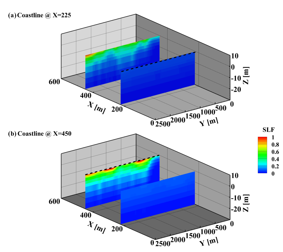
Figure A1Contours (color scale on the right) of peak SLF (t=8.4 h) as a function of the vertical Z, cross-shore X, and alongshore Y coordinates for (a) a simulation with the coastline at −0.5 m (X=225 m) and (b) a simulation with the coastline at 0 m (X=450 m). The dashed black lines mark the coastline in each respective simulation. The slice with high SLF values in panel (a) is not underneath the simulated coastline.
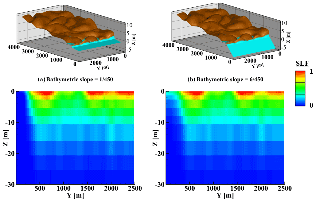
Figure A2Contours (color scale on the right) of peak SLF (t=8.4 h) for a simulation with (a) the bathymetric slope of and (b) a simulation with a higher bathymetric slope (). The upper part of each panel shows the surface with the flood water, and the lower part is the vertical slice with the SLF values below the coastline (X=450 m).
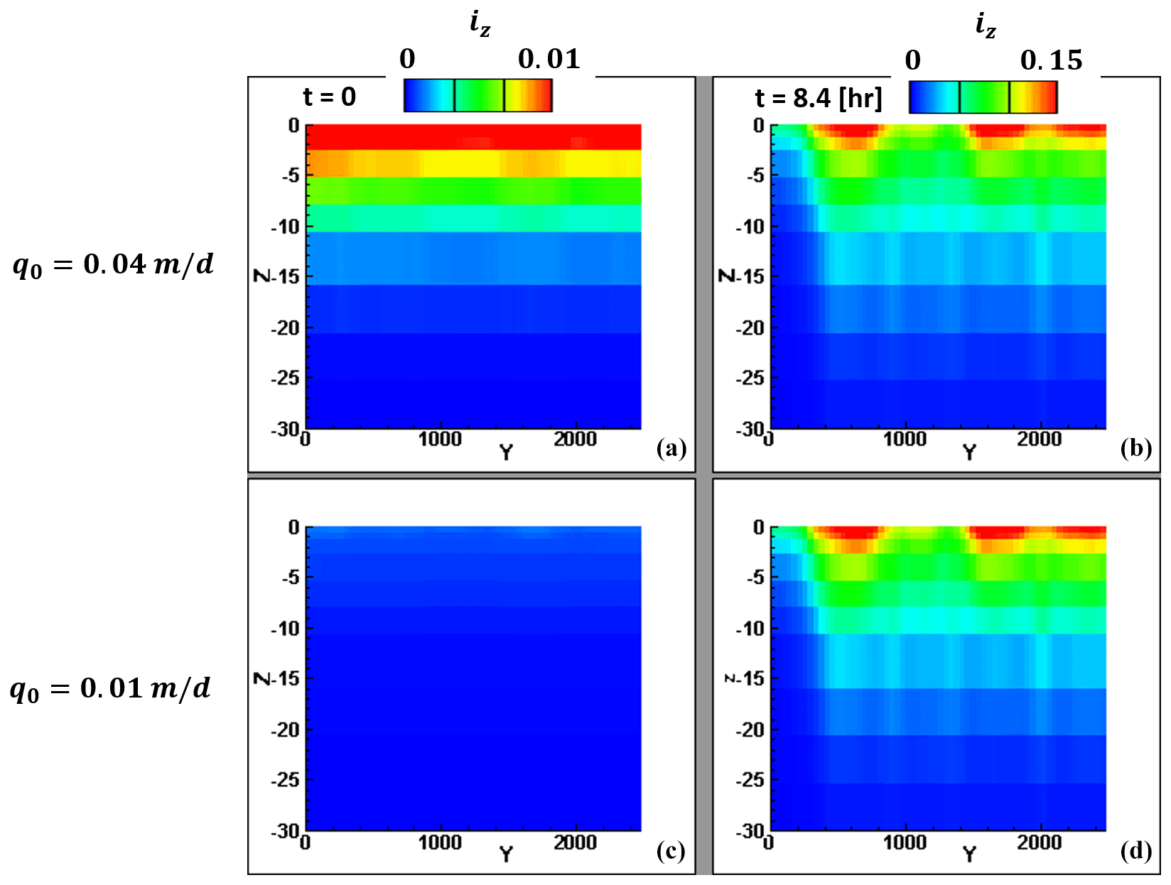
Figure A3Contours (color scale on the top) of vertical hydraulic gradients (iz) at X=450 m (shoreline location) for the pre-surge conditions (left) and the end of the surge when gradients are maximum (right) as a function of vertical Z and alongshore Y coordinates. Note the different color scales between the pre-surge (left) and peak (right) plots.
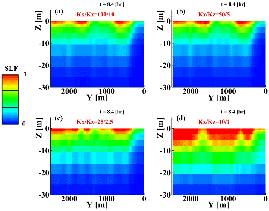
Figure A4Contours (color scale on the left) of peak SLF (t=8.4 h) vertical slices at the shoreline (X=450 m) for Kx and Kz of (a) 100 and 10, (b) 50 and 5, (c) 25 and 2.5, and (d) 10 and 1 m d−1.
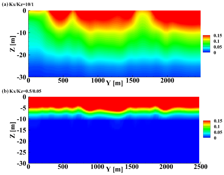
Figure A5Contours (color scale on the right) of the maximum vertical hydraulic gradients (iz) at X=450 m (shoreline location) for (a) Kz=1 and (b) Kz=0.05 as a function of vertical Z and alongshore Y coordinates.
This study used HydroGeoSphere (referenced in the reference list), which is a commercial software that can be purchased on the website of the company that develops it, Aquanty: https://www.aquanty.com/hydrogeosphere.
AP contributed through conceptualization, investigation, visualization, formal analysis, and writing of the original draft; NS contributed through conceptualization, formal analysis, writing (review and editing), and funding acquisition; MF contributed through formal analysis, and writing (review and editing); BR contributed through conceptualization, formal analysis, writing (review and editing), and funding acquisition; SE contributed through conceptualization, formal analysis, writing (review and editing), and funding acquisition; RH contributed through formal analysis, visualization, and writing (review and editing); RF contributed through formal analysis, and methodology; HM contributed through conceptualization, formal analysis, writing (review and editing), supervision, funding acquisition, and provision of resources.
The contact author has declared that none of the authors has any competing interests.
Publisher’s note: Copernicus Publications remains neutral with regard to jurisdictional claims in published maps and institutional affiliations.
This research has been supported by the National Science Foundation (grant nos. OCE1848650, OIA1757353, OCE1829136, EAR1933010, and CMMI-1751463, and a Graduate Research Fellowship) and the US Geological Survey (grant no. NIWR 2018DE01G), a Vannevar Bush Faculty Fellowship, the US Coastal Research Program, and the Woods Hole Oceanographic Institution Investment in Science Program.
This paper was edited by Albrecht Weerts and reviewed by Damien Sous and one anonymous referee.
Abdollahi, A. and Mason, H. B.: Pore Water Pressure Response during Tsunami Loading, J. Geotech. Geoenviron., https://doi.org/10.1061/(asce)gt.1943-5606.0002205, 2020.
Ataie-Ashtiani, B., Werner, A. D., Simmons, C. T., Morgan, L. K., and Lu, C.: How important is the impact of land-surface inundation on seawater intrusion caused by sea-level rise?, Hydrol. J., 21, 1673–1677, https://doi.org/10.1007/s10040-013-1021-0, 2013.
Bratton, J. F.: The Three Scales of Submarine Groundwater Flow and Discharge across Passive Continental Margins, J. Geol., 118, 565–575, https://doi.org/10.1086/655114, 2010.
Briaud, J.-L.: Geotechnical engineering: unsaturated and saturated soils. John Wiley and Sons, https://books.google.com/books?hl=en&lr=&id=6TMWDQAAQBAJ&oi=fnd&pg=PR21&dq=Geotechnical+engineering:+unsaturated+and+saturated+soils&ots=M1GNcgTZMw&sig=sw0t2K345ohBajzbl1ZVSDXGUgA#v=onepage&q=Geotechnical engineering: unsaturated and saturated soils&f=false (last access: 27 November 2022), 2013.
Burnett, W. C., Aggarwal, P. K., Aureli, A., Bokuniewicz, H., Cable, J. E., Charette, M. A., Kontar, E., Krupa, S., Kulkarni, K. M., Loveless, A., Moore, W. S., Oberdorfer, J. A., Oliveira, J., Ozyurt, N., Povinec, P., Privitera, A. M. G., Rajar, R., Ramessur, R. T., Scholten, J., Stieglitz, T., Taniguchi, M., and Turner, J. V.: Quantifying submarine groundwater discharge in the coastal zone via multiple methods, Sci. Total. Environ., 367, 498–543, https://doi.org/10.1016/j.scitotenv.2006.05.009, 2006.
Cardenas, M. B., Bennett, P. C., Zamora, P. B., Befus, K. M., Rodolfo, R. S., Cabria, H. B., and Lapus, M. R.: Devastation of aquifers from tsunami‐like storm surge by Supertyphoon Haiyan, Geophys. Res. Lett., 42, 2844–2851, 2015.
Chini, N. and Stansby, P. K. K.: Extreme values of coastal wave overtopping accounting for climate change and sea level rise, Coast. Eng., 65, 27–37, https://doi.org/10.1016/J.COASTALENG.2012.02.009, 2012.
ESRI, ArcGIS Desktop: Release 10, Redlands, CA: Environmental Systems Research Institute, Redlands, https://www.esri.com/en-us/arcgis/products/arcgis-desktop/overview (last access: 27 November 2022), 2011.
Freeze, R. A. and Cherry, J. A.: Groundwater, Prentice-Hall, https://gw-project.org/books/groundwater/ (last access: 27 November 2022), 1979.
Gelhar, L. W., Welty, C., and Rehfeldt, K. R.: A Critical Review of Data on Field-Scale Dispersion in Aquifers, Water Resour. Res., 28, 1955–1974, https://doi.org/10.1029/92WR00607, 1992.
Goren, L., Toussaint, R., Aharonov, E., Sparks, D. W., and Flekkøy, E.: A general criterion for liquefaction in granular layers with heterogeneous pore pressure, in: Poromechanics V – Proceedings of the 5th Biot Conference on Poromechanics, https://doi.org/10.1061/9780784412992.049, 2013.
Guimond, J. A. and Michael, H. A.: Effects of Marsh Migration on Flooding, Saltwater Intrusion, and Crop Yield in Coastal Agricultural Land Subject to Storm Surge Inundation, Water Resour. Res., 57, p.e2020WR028326, https://doi.org/10.1029/2020WR028326, 2021.
Iverson, R. M.: Can magma-injection and groundwater forces cause massive landslides on Hawaiian volcanoes?, J. Volcanol. Geoth. Res., 66, 295–308, 1995.
Iverson, R. M. and Major, Jon J.: Groundwater Seepage Vectors and the Potential for Hillslope Failure and Debris Flow Mobilization, Water Resour. Res., 22, 1543–1548, 1986.
Iverson, R. M. and Reid, M. E.: Gravity driven groundwater flow and slope failure potential: 1. Elastic Effective Stress Model, Water Resour. Res., 28, 925–938, https://doi.org/10.1029/91WR02694, 1992.
Mei, C. C. and Foda, M. A.: Wave-induced responses in a fluid-filled poro-elastic solid with a free surface – a boundary layer theory, Geophys. J. Int., 66, 597–631, https://doi.org/10.1111/j.1365-246X.1981.tb04892.x, 1981.
Michallet, H., Mory, M., and Piedra‐Cueva, I.: Wave-induced pore pressure measurements near a coastal structure, J. Geophys. Res.-Oceans, 114, 2009.
Mory, M., Michallet, H., Bonjean, D., Piedra-Cueva, I., Barnoud, J. M., Foray, P., Abadie, S., and Breul, P.: A field study of momentary liquefaction caused by waves around a coastal structure, B. Am. Meteorol. Soc., 133, 28–38, 2007.
Orange, D. L., Anderson, R. S., and Breen, N. A.: Regular Canyon Spacing in the Submarine Environment: The Link Between Hydrology and Geomorphology, Geol. Soc. Am. Bull., 4, 35–39, 1994.
Orange, D. L., Yun, J., Maher, N., Barry, J., and Greene, G.: Tracking California seafloor seeps with bathymetry, backscatter and ROVs, Cont. Shelf Res., 22, 2273–2290, https://doi.org/10.1016/S0278-4343(02)00054-7, 2002.
Paldor, A. and Michael, H. A.: Storm Surges Cause Simultaneous Salinization and Freshening of Coastal Aquifers, Exacerbated by Climate Change, Water Resour. Res., 57, e2020WR029213, https://doi.org/10.1029/2020WR029213, 2021.
Paldor, A., Aharonov, E., and Katz, O.: Thermo-haline circulations in subsea confined aquifers produce saline, steady-state deep submarine groundwater discharge, J. Hydrol., 580, p.124276, https://doi.org/10.1016/j.jhydrol.2019.124276, 2020.
Paldor, A., Frederiks, R. S., and Michael, H. A.: Dynamic Steady State in Coastal Aquifers Is Driven by Multi-Scale Cyclical Processes, Controlled by Aquifer Storativity, Geophys. Res. Lett., 49, e2022GL098599, https://doi.org/10.1029/2022GL098599, 2022.
Robinson, C., Xin, P., Li, L., and Barry, D. A.: Groundwater flow and salt transport in a subterranean estuary driven by intensified wave conditions, Water Resour. Res., 50, 165–181, 2014.
Rozhko, A. Y., Podladchikov, Y. Y., and Renard, F.: Failure patterns caused by localized rise in pore-fluid overpressure and effective strength of rocks, Geophys. Res. Lett., 34, L22304, https://doi.org/10.1029/2007GL031696, 2007.
Sakai, T., Hatanaka, K., and Mase, H.: Wave-induced effective stress in seabed and its momentary liquefaction. Journal of Waterway, Port, Coastal and Ocean Engineering, 118, 202–206, https://doi.org/10.1061/(ASCE)0733-950X(1992)118:2(202), 1992.
Schorghofer, N., Jensen, B., Kudrolli, A., and Rothman, D. H.: Spontaneous channelization in permeable ground: theory, experiment, and observation, J. Fluid Mech., 503, 357–374, https://doi.org/10.1017/S0022112004007931, 2004.
Sous, D., Lambert, A., Rey, V., and Michallet, H.: Swash-groundwater dynamics in a sandy beach laboratory experiment, Coast. Eng., 80, 122–136, https://doi.org/10.1016/j.coastaleng.2013.05.006, 2013.
Sous, D., Petitjean, L., Bouchette, F., Rey, V., Meulé, S., Sabatier, F., and Martins, K.: Field evidence of swash groundwater circulation in the microtidal rousty beach, France, Adv. Water Resour., 97, 144–155, https://doi.org/10.1016/j.advwatres.2016.09.009, 2016.
Stegmann, S., Sultan, N., Kopf, a., Apprioual, R., and Pelleau, P.: Hydrogeology and its effect on slope stability along the coastal aquifer of Nice, France, Mar. Geol., 280, 168–181, https://doi.org/10.1016/j.margeo.2010.12.009, 2011.
Tebaldi, C., Strauss, B. H., and Zervas, C. E.: Modelling sea level rise impacts on storm surges along US coasts, Environ. Res. Lett., 7, p.014032, https://doi.org/10.1088/1748-9326/7/1/014032, 2012.
Therrien, R., McLaren, R. G., Sudicky, E. A., and Panday, S. M.: HydroGeoSphere. A three-dimensional numerical model describing fully-integrated subsurface and surface flow and solute transport. Groundwater Simulations Group, https://www.aquanty.com/hydrogeospheresw (last access: 27 November 2022), 2010.
Turner, I. L., Rau, G. C., Austin, M. J., and Andersen, M. S.: Groundwater fluxes and flow paths within coastal barriers: Observations from a large-scale laboratory experiment (BARDEX II), Coast. Eng., 113, 104–116, https://doi.org/10.1016/j.coastaleng.2015.08.004, 2016.
Yang, J., Graf, T., Herold, M., and Ptak, T.: Modelling the effects of tides and storm surges on coastal aquifers using a coupled surface-subsurface approach, J. Contam. Hydrol., 149, 61–75, https://doi.org/10.1016/j.jconhyd.2013.03.002, 2013.
Yang, J., Zhang, H., Yu, X., Graf, T., and Michael, H. A.: Impact of hydrogeological factors on groundwater salinization due to ocean-surge inundation, Adv. Water Resour., 111, 423–434, https://doi.org/10.1016/J.ADVWATRES.2017.11.017, 2018.
Yang, S. and Tsai, F. T. C.: Understanding impacts of groundwater dynamics on flooding and levees in Greater New Orleans, Journal of Hydrology: Regional Studies, 32, p.100740, https://doi.org/10.1016/j.ejrh.2020.100740, 2020.
Yeh, H. and Mason, H. B.: Sediment response to tsunami loading: Mechanisms and estimates, Geotechnique, 64, 131–143, https://doi.org/10.1680/geot.13.P.033, 2014.
Yu, X., Yang, J., Graf, T., Koneshloo, M., O'Neal, M. A., and Michael, H. A.: Impact of topography on groundwater salinization due to ocean surge inundation, Water Resour. Res., 52, 5794–5812, https://doi.org/10.1002/2016WR018814, 2016.
Zen, K., Jeng, D. S., Hsu, J. R. C., and Ohyama, T.: Wave-induced seabed instability: Difference between liquefaction and shear failure, Soils Found., 38, 37–47, https://doi.org/10.3208/sandf.38.2_37, 1998.
Zinn, B. and Harvey, C. F.: When good statistical models of aquifer heterogeneity go bad: A comparison of flow, dispersion, and mass transfer in connected and multivariate Gaussian hydraulic conductivity fields, Water Resour. Res., 39, https://doi.org/10.1029/2001WR001146, 2013.