the Creative Commons Attribution 4.0 License.
the Creative Commons Attribution 4.0 License.
 | 02 Dec 2022
Coupling a global glacier model to a global hydrological model prevents underestimation of glacier runoff
Pau Wiersma
Jerom Aerts
Harry Zekollari
Markus Hrachowitz
Niels Drost
Matthias Huss
Edwin H. Sutanudjaja
Global hydrological models have become a valuable tool for a range of global impact studies related to water resources. However, glacier parameterization is often simplistic or non-existent in global hydrological models. By contrast, global glacier models do represent complex glacier dynamics and glacier evolution, and as such, they hold the promise of better resolving glacier runoff estimates. In this study, we test the hypothesis that coupling a global glacier model with a global hydrological model leads to a more realistic glacier representation and, consequently, to improved runoff predictions in the global hydrological model. To this end, the Global Glacier Evolution Model (GloGEM) is coupled with the PCRaster GLOBal Water Balance model, version 2.0 (PCR-GLOBWB 2), using the eWaterCycle platform. For the period 2001–2012, the coupled model is evaluated against the uncoupled PCR-GLOBWB 2 in 25 large-scale (>50 000 km2), glacierized basins. The coupled model produces higher runoff estimates across all basins and throughout the melt season. In summer, the runoff differences range from 0.07 % for weakly glacier-influenced basins to 252 % for strongly glacier-influenced basins. The difference can primarily be explained by PCR-GLOBWB 2 not accounting for glacier flow and glacier mass loss, thereby causing an underestimation of glacier runoff. The coupled model performs better in reproducing basin runoff observations mostly in strongly glacier-influenced basins, which is where the coupling has the most impact. This study underlines the importance of glacier representation in global hydrological models and demonstrates the potential of coupling a global hydrological model with a global glacier model for better glacier representation and runoff predictions in glacierized basins.
- Article
(6332 KB) - Full-text XML
-
Supplement
(13647 KB) - BibTeX
- EndNote


A total of 1.9 billion people worldwide rely on glacial meltwater as part of their water resources (Immerzeel et al., 2020). Glaciers can act as a crucial multiannual buffer, particularly in regions prone to drought (Pritchard, 2019; Biemans et al., 2019). Yet, as glaciers have been strongly retreating (Hugonnet et al., 2021) and are projected to continue to do so throughout the 21st century (Edwards et al., 2021), their role in the water cycle will change. On the intra-annual scale, peak runoff will occur earlier in summer, while on the interannual scale, glacier mass loss will cause an initial peak in glacier runoff, followed by a steady decline until a new equilibrium is reached (Jansson et al., 2003; Huss and Hock, 2018). In many basins throughout the world, this “peak water” already lies in the past (Huss and Hock, 2018), indicating that the shift from a glacial to a nival–pluvial regime is well underway. This will not only impact the water supply of millions of people but will also lead to an increased potential for natural hazards, hydro-political tension (Immerzeel et al., 2020), and instability of many ecosystems influenced by glacial meltwaters (Cauvy-Fraunié and Dangles, 2019).
To be able to account for the changing contribution of glaciers to daily runoff, many hydrological models applied to glacierized catchments include glacier parameterization schemes to form glacio-hydrological models (see van Tiel et al., 2020 for an overview). These models have been applied both at a small-catchment scale (e.g., Huss et al., 2008; Ragettli et al., 2016) as well as at a regional- or multiple-catchment scale (e.g., Farinotti et al., 2012; Frans et al., 2018). Another approach involves the use of glacier geometry evolution estimates of an independent glacier model as forcing to a hydrological model, which has likewise been applied at local (Laurent et al., 2020; Hanus et al., 2021) to regional (Brunner et al., 2019) scales.
On a global scale, however, the integration of glacier processes in hydrological modeling is still lacking. Global hydrological models (GHMs) have gained popularity in recent years and have been used to study many different global issues, including flood hazards (e.g., Do et al., 2020; Aerts et al., 2020), drought propagation (e.g., Gevaert et al., 2018), and ecological degradation (e.g., Barbarossa et al., 2021). Nonetheless, GHMs are reported to have an overly simplistic description of glacier dynamics (Van Dijk et al., 2014; Cáceres et al., 2020) and to mostly treat glaciers as non-glacierized terrain (Cáceres et al., 2020). The complex and dynamic contribution of glacier runoff to basin runoff is therefore expected to be captured only to a limited degree by GHMs. This has been shown to cause problems in the application of GHMs to glacierized basins (Scanlon et al., 2018; Müller Schmied et al., 2021).
Models dedicated to simulating glacier evolution on a global scale exist in the form of global glacier models (GGMs) (Hock et al., 2019; Marzeion et al., 2020). These models combine a surface mass balance model with a glacier geometry change model, which can range in complexity from a volume–area–length scaling model (Marzeion et al., 2012; Radić and Hock, 2014) to a mass-conserving retreat parameterization (Huss and Hock, 2015) to a prognostic ice dynamical model (Maussion et al., 2019; Zekollari et al., 2019). Although most GGMs are developed with the goal of simulating the mass balance and evolution of glaciers, some also produce glacier runoff as a model output (Hirabayashi et al., 2010; Bliss et al., 2014; Huss and Hock, 2018). This makes them suitable for coupling with GHMs, where glacier runoff can potentially be used as a direct input.
Several studies have investigated the global contribution of glaciers to streamflow on a coarse temporal resolution. Kaser et al. (2010) compared glacier runoff with the mean upstream precipitation at several elevations to estimate the contribution of glacier runoff along the course of a multitude of large glacier-fed rivers. To a similar purpose, Schaner et al. (2012) used a land-surface hydrological model combined with an energy-balance model. Huss and Hock (2018) compared the runoff of a GGM to monthly average basin runoff observations to assess the changing contribution to basin-scale runoff and the timing of intra- and interannual peak water. In another recent study, Cáceres et al. (2020) coupled a GGM with a GHM to assess the joint contribution of glacial and non-glacial water storage anomalies to ocean mass change. However, to the best of our knowledge, no study so far has investigated whether global runoff predictions can be improved through the coupling of GHMs and GGMs.
In this study, we test the hypothesis that the coupling of a GGM with a GHM can lead to a more realistic glacier representation and, consequently, to improved daily runoff estimates by GHMs in glacierized basins. To this end, the GGM GloGEM (Global Glacier Evolution Model) (Huss and Hock, 2015) is coupled with the GHM PCR-GLOBWB 2 (PCRaster GLOBal Water Balance model: version 2.0) (Sutanudjaja et al., 2018). We evaluate the coupled model for 25 large, glacierized basins (>50 000 km2) in North and South America, Europe, Asia, and New Zealand through a comparison with the uncoupled GHM, which serves as a benchmark. Through this approach, we aim to identify structural differences in behavior between the two models as well as to determine which model is the most suited to reproducing the observed basin runoff. To benefit its replicability with other GHMs, we apply a simplified coupling method using standard open-source libraries. We expect the gain in the glacier representation accuracy of the GGM relative to the GHM to compensate for any loss in physical basis following the simplifications applied in the coupling method.
2.1 Global hydrological model
For the global hydrological modeling, we used PCR-GLOBWB 2 (PCRaster GLOBal Water Balance model: version 2.0) (Sutanudjaja et al., 2018), which can be considered a representative example of a GHM in terms of snow and glacier modeling. Compared to other GHMs, it has the advantage of a relatively high resolution (5 arcmin, or 10 km at the Equator) and the ability to integrate human water use. Details on the model can be found in Sutanudjaja et al. (2018) and Beek et al. (2011). The four standard land cover types are tall natural vegetation, short natural vegetation, non-paddy irrigated crops, and paddy irrigated crops, and there is an option to include custom land cover types. For latitudes up to 60∘, PRC-GLOBWB 2 relies on the digital elevation model (DEM) of HydroSHEDS (Lehner et al., 2008), while for latitudes over 60∘, the lower-resolution HYDRO1K DEM of USGS is used (Verdin and Greenlee, 1998). The snow module of PCR-GLOBWB is based on the HBV snow module (Bergström, 1995) and accounts for accumulation, melt, and refreezing using a degree-day method, but no redistribution (e.g., sliding of the snowpack, avalanches) to other grid cells is considered. Glaciers are effectively treated as static rock masses – i.e., the DEMs reflect the glacier surface elevation, but glacier flow, snow compression and ablation are not resolved. For the sake of consistency with the GGM, ERA-Interim reanalysis temperature and precipitation data (Dee et al., 2011) are used as forcing. Of note is that PRC-GLOBWB 2 requires no subsequent calibration.
2.2 Global glacier model
The Global Glacier Evolution Model (GloGEM) was developed by Huss and Hock (2015), while the data we use here are from a more recent study (Huss and Hock, 2018) that specifically focused on glacier runoff. The data consist of the runoff of individual glaciers in the 56 glacierized drainage basins across five continents, with an area of more than 50 000 km2, a glacier area of more than 30 km2, and an ice cover of more than 0.01 % of the basin area. The glacier runoff is defined as the total amount of water originating from the glacierized area defined in the Randolph Glacier Inventory (RGI) (Pfeffer et al., 2014) and is kept constant – i.e., runoff from the areas that become ice-free throughout the simulation remains accounted for. GloGEM was run for the period 1980–2100, but here, we only consider the simulation results from 2000–2012. This time interval for the present analysis is given by the first inventory date of most of the RGI glacier outlines used in GloGEM (Pfeffer et al., 2014) and the last year for which ERA-Interim reanalysis forcing data were used. After conversion to hydrological years, the considered date range thus becomes October (April) 2000 to September (March) 2012 for the Northern (Southern) Hemisphere.
The glacier runoff data, which are resolved at the level of individual glaciers, were preprocessed to match the spatial and temporal resolution of PCR-GLOBWB 2. This consisted of a conversion to raster data of the same resolution as PCR-GLOBWB 2 (5 arcmin) and, consequently, a resampling from monthly to daily resolution. The resampling was performed with a weighting function based on the ERA-Interim surface temperature data (Eqs. 1 and 2). Only days with a daily mean temperature below −5 ∘C were excluded from the weighting, since melt can still occur on days with a mean air temperature below 0 ∘C due to strong irradiation (Ayala et al., 2017) or a positive maximum temperature. Despite the existence of a strong day–night cycle over glaciers, a resampling to diurnal resolution was not possible given the daily time step of PCR-GLOBWB 2.
Here, wD is the weight given to a particular day; TD is the mean daily surface temperature in K; is the average of all mean daily temperatures above 268 K in the considered month; and NT>268 is the number of days with a mean daily temperature above 268 K. α is a weighting factor that was set to 20 after calibration on the runoff of the Great Aletsch Glacier (BAFU, 2020) (see Fig. S1 in the Supplement). A sensitivity analysis of α is given in Sect. S6 in the Supplement. Finally, RD and RM are the daily and monthly grid cell glacier runoff, respectively. This weighting function is mass conserving, since it is linear in nature and since the sum of the weights always equals NT>268,
2.3 Model platform
We generated all model-specific ERA-Interim forcing data and performed all model coupling and model runs within the eWaterCycle platform (Hut et al., 2022). The eWaterCycle platform is a hydrological modeling platform that aims to improve the accessibility and reproducibility of hydrological models. On the eWaterCycle platform, hydrological models are run in containers and “communicate” with the central experiment that runs in a Jupyter Notebook. Communication with hydrological models is independent of the model language through BMI (Hutton et al., 2020) and GRPC4BMI (van den Oord et al., 2019). Additionally, the ESMValTool (Eyring et al., 2016) implementation in eWaterCycle allows for smooth preprocessing and high compatibility of forcing data.
2.4 Basin runoff observations
Runoff observation data were obtained through the Global Runoff Data Centre (GRDC, 2020) for all basins except for the Rhone, for which we used observations from the French national hydrological service (Hydrobanque, 2020). Out of the 56 basins used by Huss and Hock (2018), 30 are present in the GRDC database, with more than five years of daily runoff observations between 2000 and 2012. If a basin contained more than one gauging station in the GRDC database, we automatically selected the most upstream station that still included all the basin's glacier runoff, hereafter called the glacier sink (e.g., for the Rhine, the gauging station in Basel was chosen instead of the most downstream station at Lobith). The glacier sinks were found using HydroSHEDS (Lehner et al., 2008). If the only available station was upstream of the glacier sink, we excluded the glaciers downstream of that station from our analysis. While the GRDC database does contain stations along the Rhone in Switzerland, the glacier sink is near the river mouth at Beaucaire. Therefore, observations at Beaucaire from the Hydrobanque were used as an alternative. The Supplement contains more information on the GRDC station numbers and the available years as well as a detailed map of all basins, their glacier coverage, and the location of the gauging stations.
Of the 30 resulting basins, 5 were discarded from analysis for various issues related to river routing (see Sect. S5). The remaining 25 large-scale, glacierized basins are mostly concentrated in northwestern America and Europe (Fig. 1). Openly available runoff data from rivers originating in the Himalayas are scarce, despite many of them being some of the world's most important and vulnerable glacier-fed river basins (Immerzeel et al., 2020). (Seasonally) arid regions are likewise underrepresented, the only exceptions being the Rhone and the Negro river (respectively Cfb/Csa and Csb/Bsk on the Köppen–Geiger climate classification scale, Kottek et al., 2006). On a practical note, since the vast majority of basins are located in the Northern Hemisphere, we will only mention the Northern Hemisphere months in the remainder of this work. The Southern Hemisphere equivalents will be implied for the Amazon, Negro, and Clutha basins.
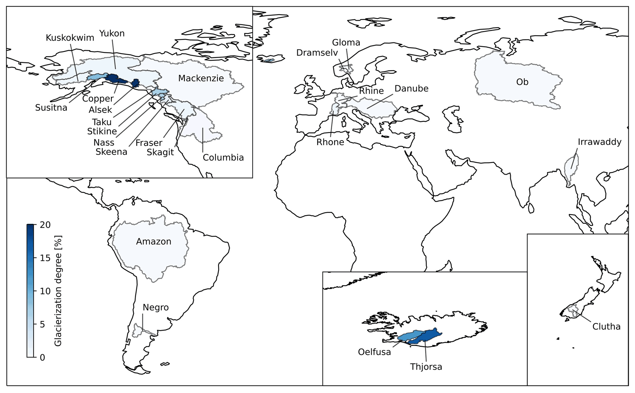
Figure 1The 25 large-scale (>50 000 km2), glacierized basins for which sufficient runoff observations are found. The hue represents the fraction of basin area covered by glaciers.
3.1 Model coupling
Within the context of this study, the term “coupling” refers to the replacement of the PCR-GLOBWB 2 runoff by the GloGEM runoff for glacierized areas. We deem this simplification of coupling to be physically plausible, since much of the exchange of water between glaciers and the rest of the catchment occurs at the surface in the form of runoff. To the best of our knowledge, this coupling approach has not been applied before for glacio-hydrological modeling purposes. Several situations can be thought of for which further coupling between a glacier model and a hydrological model could be applied, such as surging glaciers damming upstream rivers (Sevestre and Benn, 2015) or the flow of subglacial groundwater (Vincent et al., 2019), but these are considered irrelevant at the considered scale.
To ignore the PCR-GLOBWB 2 runoff originating from glacierized areas, we removed the fraction of the PCR-GLOBWB 2 land cover that corresponds to the glacierized area of the Randolph glacier inventory. This fraction is calculated per grid cell and subtracted from the short natural vegetation land cover class, since it is in the vast majority of cases the only land cover class present in glacierized grid cells. This operation prevents the PCR-GLOBWB 2 land cover classes from adding up to 1:
Effectively, this causes PCR-GLOBWB 2 to omit any calculations on the glacier-covered area without having to adjust the source code or forcing and without having to create a new land cover class. By not changing the source code, the reproducibility of this approach with other GHMs is increased. The only additional adjustment to be made was the disabling of the PCR-GLOBWB 2 setting that ensures that the sum of land cover classes is 1.
As for the coupling itself, for each time step, the GloGEM glacier runoff was added to the PCR-GLOBWB 2 variable channel_storage, which is equivalent to a direct routing into the stream. This is a simplification, since both under the glacier and below the glacier, terminus groundwater infiltration is possible under certain conditions (Vincent et al., 2019; Castellazzi et al., 2019). Nevertheless, given the large scope of this study and the lacking research on this topic (Vincent et al., 2019), we ignored glacial groundwater recharge.
The numerical implementation of the coupling is largely done using standard BMI functionality. As mentioned in Sect. 2.3, the eWaterCycle platform uses BMI for communication with the hydrological models and therefore also allows for requesting and modifying model variables using the get_value() and set_value() BMI functions. In this case, these functions are used to add the GloGEM glacier runoff to PCR-GLOBWB 2, but other combinations of glacier and hydrological models could be coupled using the same interface. While the adjusted land cover fraction maps need to be created manually, they are passed to the model via the model's configuration file in the BMI initialize() function.
3.2 Model setups
Three different model setups were used. The benchmark is the default PCR-GLOBWB 2 model. The coupled model omits the PCR-GLOBWB 2 glacierized area and applies the GloGEM coupling instead (as discussed in Sect. 3.1). Finally, the bare model is an auxiliary model setup that omits the PCR-GLOBWB 2 glacierized area but does not apply the GloGEM coupling. In theory, the difference between the benchmark and the bare model results in the routed PCR-GLOBWB 2 runoff for glacier-covered areas, while the difference between the coupled and the bare model is equal to the routed GloGEM runoff. We assumed the bare model to not include any glacier runoff. To initialize the models, one year with the climatological average of the period 1990–1999 was repeated 50 times as a model spin-up (Sutanudjaja et al., 2018). All model setups are run between the hydrological years 2000–2012. As PCR-GLOBWB 2 is not calibrated, the simulation over these 12 years can be seen as a test for the prediction quality of the coupled model versus the uncoupled model.
3.3 Spilling prevention
Through the conversion of the basin boundaries from vector to raster format, a considerable part of the glaciers ended up in grid cells that were at the risk of being routed into adjacent basins, causing the runoff of these glaciers to be “spilled”. To neutralize this spilling, the runoff of these glaciers was transferred to downstream grid cells that did not intersect with the basin vector boundary. This spilling prevention was only applied to the coupled model and not to the benchmark, effectively leading to a larger total basin area for the coupled model (0 %–2 % larger across all basins).
3.4 Evaluation metrics
3.4.1 Evaluation against the benchmark
To identify differences in basin runoff between the coupled model and the benchmark as a function of the time of the year, we applied the following normalized difference metric over all 25 basins:
in which ND stands for the normalized difference; d is the calendar day; Q is the basin runoff (in m3 s−1); and q99 is the 99th percentile of the difference taken over the whole time range. The normalization was applied with the 99th percentile instead of the maximum difference to avoid the influence of extreme maxima. With this metric, a positive value indicates that, on average, the coupled model produces higher discharge than the benchmark on that particular calendar day, and vice versa.
3.4.2 Evaluation against observations
In the evaluation against the basin runoff observations, the difference in performance between the coupled model and the benchmark should be expressed relative to the highest possible performance difference (Seibert et al., 2018). After all, the same absolute error difference has larger implications on a day with little glacier melt than at the peak of the melt season. Since, in this study, the difference between the two models can only be attributed to a difference in glacier representation, we took the difference between zero glacier runoff and the maximum glacier runoff among PCR-GLOBWB 2 and GloGEM as the maximum possible performance difference. This corresponds to the maximum difference among PCR-GLOBWB 2 and GloGEM with the bare model (see Sect. 3.2). The performance difference between the coupled model and the benchmark can then be expressed relative to the maximum possible performance difference as follows:
in which RMSE entails the root of the mean squared error, and RRD is the relative RMSE difference. With the RRD, a positive sign indicates that the coupled model performs better compared to the benchmark, and vice versa, while the value indicates the fraction of the difference to the maximum possible difference. The RRD is therefore always between −1 and 1. A further justification of the metric choice is given in Sect. S4.
3.4.3 Glacier influence metric
While the glacierization degree can give some indication of the hydrological importance of the glaciers in a river basin (Zhang et al., 2016; He et al., 2021), we used the results of the coupled model to formulate a direct measure of the importance of glacier runoff on the basin scale. It is defined as the 99th percentile of the routed GloGEM runoff contribution to the coupled model daily runoff (GC99). The 99th percentile is chosen to reflect the crucial role of glaciers under extreme droughts (Huss, 2011). The threshold to distinguish weakly glacier-influenced basins from strongly glacier-influenced basins is chosen arbitrarily at GC99=0.5. In other words, in strongly glacier-influenced basins, glacier runoff makes up more than 50 % of the total basin runoff in 1 % of the days. Out of 25 basins, this gives 9 strongly glacier-influenced basins between Susitna (GC=0.50) and Oelfusa (GC99=0.85) and 16 weakly glacier-influenced basins between Amazon (GC99=0.003) and Kuskokwim (GC99=0.35).
4.1 Hydrograph analysis
While 12 years of basin runoff are simulated for all 25 basins, we constrict the hydrograph analysis in this section to one representative year for 6 basins covering the full range of glacierization (Fig. 2). The complete collection of hydrographs is presented in Sect. S8.
In weakly glacier-influenced basins (Mackenzie, Rhine, Columbia) the benchmark and the coupled model produce nearly indistinguishable results at the basin scale. This is also the case for the Rhone basin, where the strong glacier influence is only manifested in dry summers (e.g., 2003). The remaining strongly glacier-influenced basins (Alsek, Oelfusa) reveal that the coupled model produces higher runoff than the benchmark during the melt season. Compared to the runoff observations, the benchmark has the tendency to overestimate the melt season runoff in weakly glacier-influenced basins, and vice versa for strongly glacier-influenced basins. Finally, in certain basins (e.g., Oelfusa, Columbia), the difference between the benchmark and the bare model is minimal, meaning that PCR-GLOBWB 2 generates virtually no runoff from glacierized areas in these basins.
The result of the resampling of the GloGEM glacier runoff from monthly to daily resolution (see Sect. 2.2) is shown on the inverted axis of Fig. 2. Within each month, the daily glacier runoff fluctuations are deemed realistic, but between months, sudden and rather unrealistic variations are visible (e.g., May to June for Mackenzie). These variations are a consequence of the resampling having been performed for each month independently. A higher weighting factor α could potentially increase the sensitivity of the resampling to temperature and smooth out the jumps, although a sensitivity analysis demonstrates that this artifact does not significantly influence the runoff results (see Sect. S6).
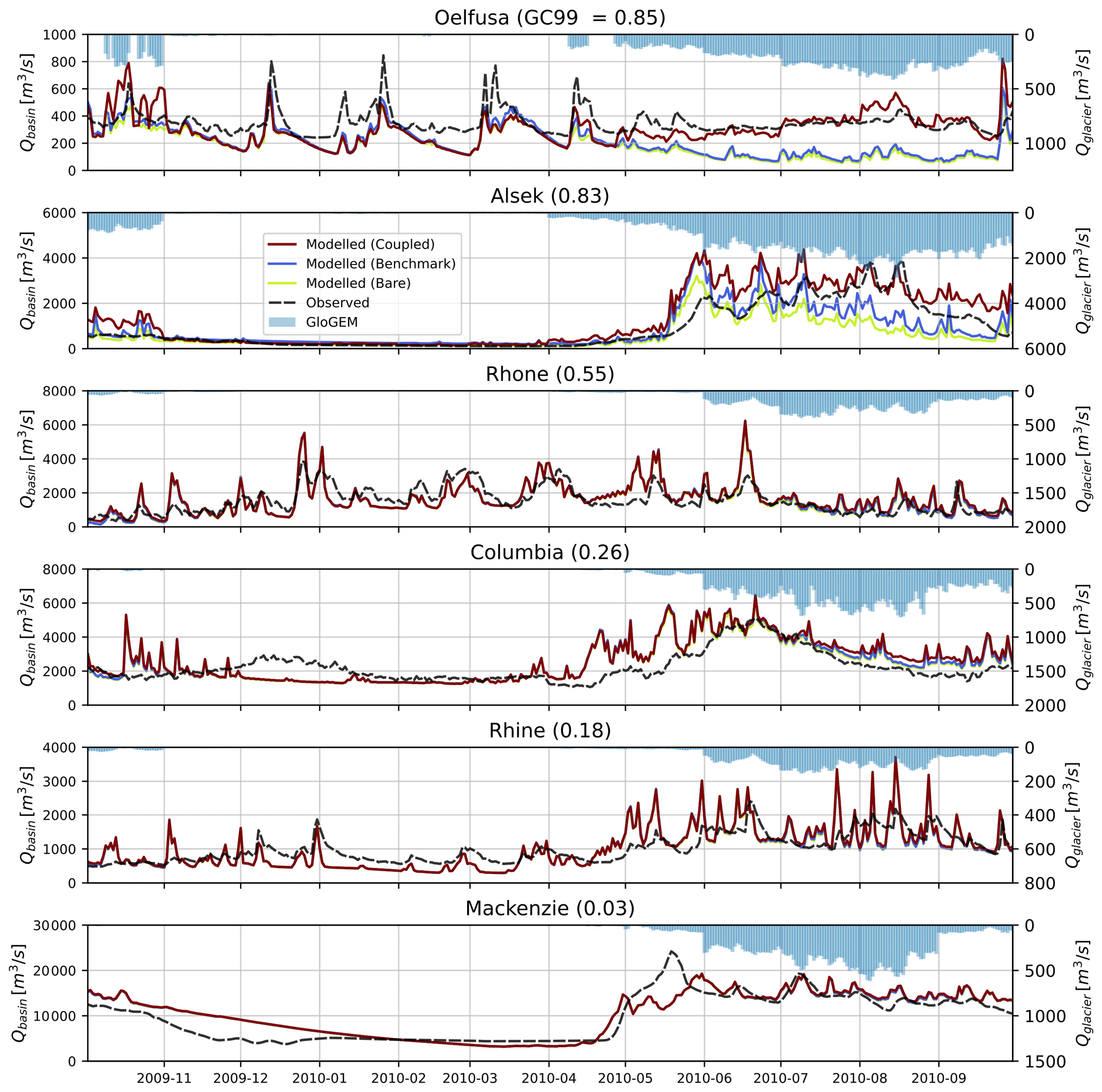
Figure 2Modeled and observed runoff of a representative selection of the 25 basins for a year close to average conditions. The left y axis represents the runoff at the selected gauging station, while the right y axis represents the GloGEM total basin glacier runoff. Note the different extents per basin on the y axes. The 99th percentile of the GloGEM contribution to the coupled model daily runoff is presented with the basin name. The remaining hydrographs are presented in Sect. S8.
4.2 Evaluation against the benchmark
The coupled model produces higher basin runoff than the benchmark for all basins throughout the melting season (Fig. 3a). The ND shows a general pattern throughout the year for most basins, with an increase from May to July, a peak in August, and a decrease in September and October. Only a few weakly glacier-influenced basins (i.e., Amazon, Ob, and Negro) deviate from this pattern. However, some basins (Fraser, Susitna, Kuskokwim) show slightly negative ND-values in May and October, indicating that, here, the coupled model temporarily produces lower runoff than the benchmark.
While the general ND pattern is shared by nearly all basins, the impact this difference has on the total simulated runoff is greater in strongly glacier-influenced basins (Fig. 3b). In the Amazon, the coupled model runoff at the peak of the melt season (July and August in N.H.) is only 0.07 % higher than the benchmark runoff, while in the Oelfusa, this difference in peak runoff exceeds 250 %.
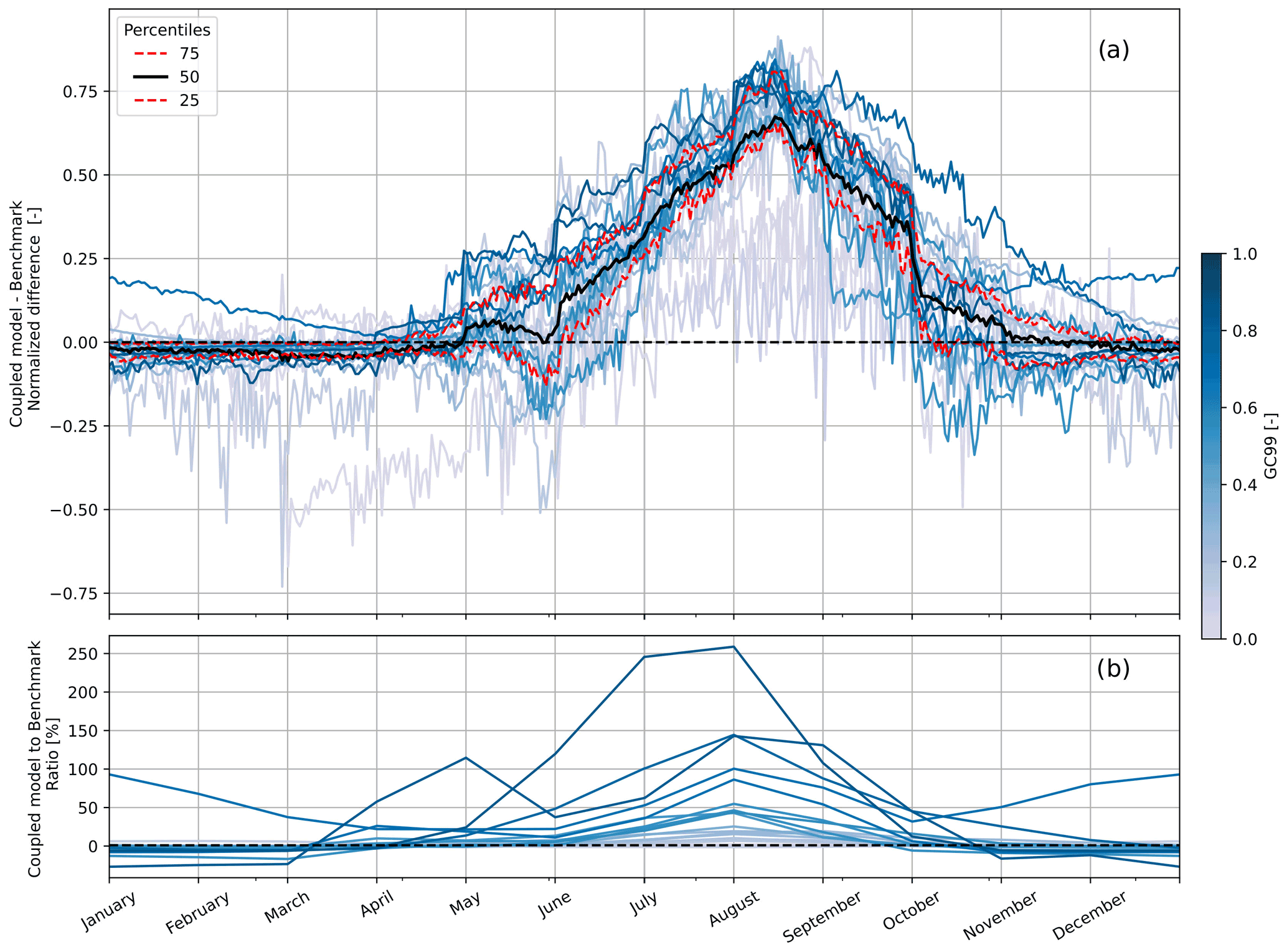
Figure 3(a) Mean normalized difference (ND) between the coupled model (PCR GLOBWB 2 and GloGEM) and the benchmark (only PCR-GLOBWB 2) for all 25 basins, showing that the coupled model produces higher runoff estimates throughout the melt season. The normalization is performed against the 99th percentile of the difference over the whole time range (2001–2012). The mean is computed for each calendar day over the same period. The solid black and dashed red lines represent the quartiles among the 25 basins. (b) Ratio of the coupled model to the benchmark, averaged per month and over the period 2001–2012. The blue hue in both figures represents the 99th percentile of the routed GloGEM glacier runoff contribution to the coupled model runoff (GC99). The data of the three Southern Hemisphere basins are shifted six months forward in time to match the Northern Hemisphere months on the x axis.
4.3 Evaluation against observations
Over all basins, the coupled model performs worse than the benchmark in terms of matching the observations. This is indicated by the mostly negative RRD scores (57 % RRD scores<0, Fig. 4). However, when only considering the nine strongly glacier-influenced basins (GC99>0.5), the coupled model performs better ( RRD-scores>0). This is particularly the case in July and August, at the peak of the ice melt season ( RRD-scores>0). Furthermore, the average performance difference varies per month. Compared to the benchmark, the coupled model performs best in May ( RRD-scores>0) and worst in September ( RRD-scores>0). The coefficient of correlation (R2) suggests a weak correlation of RRD scores with glacier contribution for July and August but no correlation for the other months. Note that the highest performance gain for the coupled model is achieved at the basin with the strongest glacier influence (Oelfusa, RRD-scores>0).
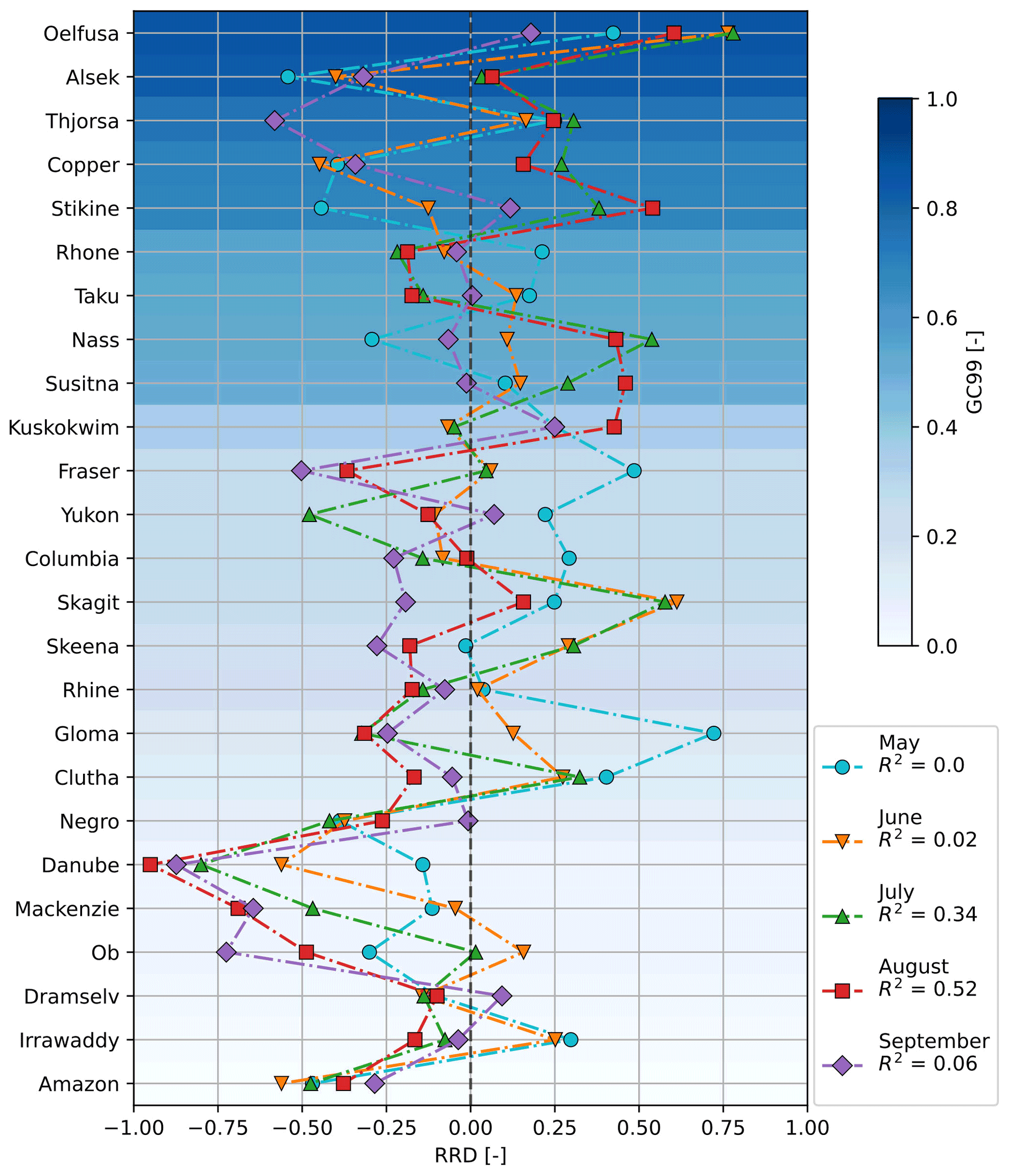
Figure 4The relative RMSE difference (RRD) over all 25 basins throughout the melt season. The RMSE difference is calculated relative to the routed glacier runoff, which embodies the maximum possible RMSE difference. Positive scores indicate an improvement of the coupled model over the benchmark compared to observed runoff, and vice versa. The RRD always lies between −1 and 1. The basins are sorted based on the 99th percentile of the contribution of the routed GloGEM glacier runoff to the coupled model runoff (GC99). The coefficients of determination (R2) represent the correlation of RRD scores with the glacier contribution. The months are given only for the Northern Hemisphere, but the results of the three Southern Hemisphere basins are shown for November–March. The distinction between strongly and weakly glacier-influenced basins is set between Sustina and Kuskokwim (GC=0.5).
A stand-alone performance evaluation of PCR-GLOBWB 2 is presented in Fig. S2, showing positive Nash–Sutcliffe efficiency values (Nash and Sutcliffe, 1970) for basins with seasonal runoff regimes but negative calendar day benchmark efficiency values (Schaefli and Gupta, 2007) for all basins except the Rhone. Furthermore, the results of three alternatives to the RRD metric, along with an explanation on why these metrics were not deemed suitable for this particular study, are given in Sect. S4.
5.1 Evaluation against the benchmark
5.1.1 Overall difference
For four geographically representative basins, we have identified several possible mechanisms to explain the overall runoff difference between the coupled model and the benchmark (Fig. 5). These mechanisms have been quantified on an annual basis to examine their contribution to the runoff difference. Since the coupling only applies to the glacier-covered area, the difference can only be attributed to the different representation of glaciers and the meteorological forcing.
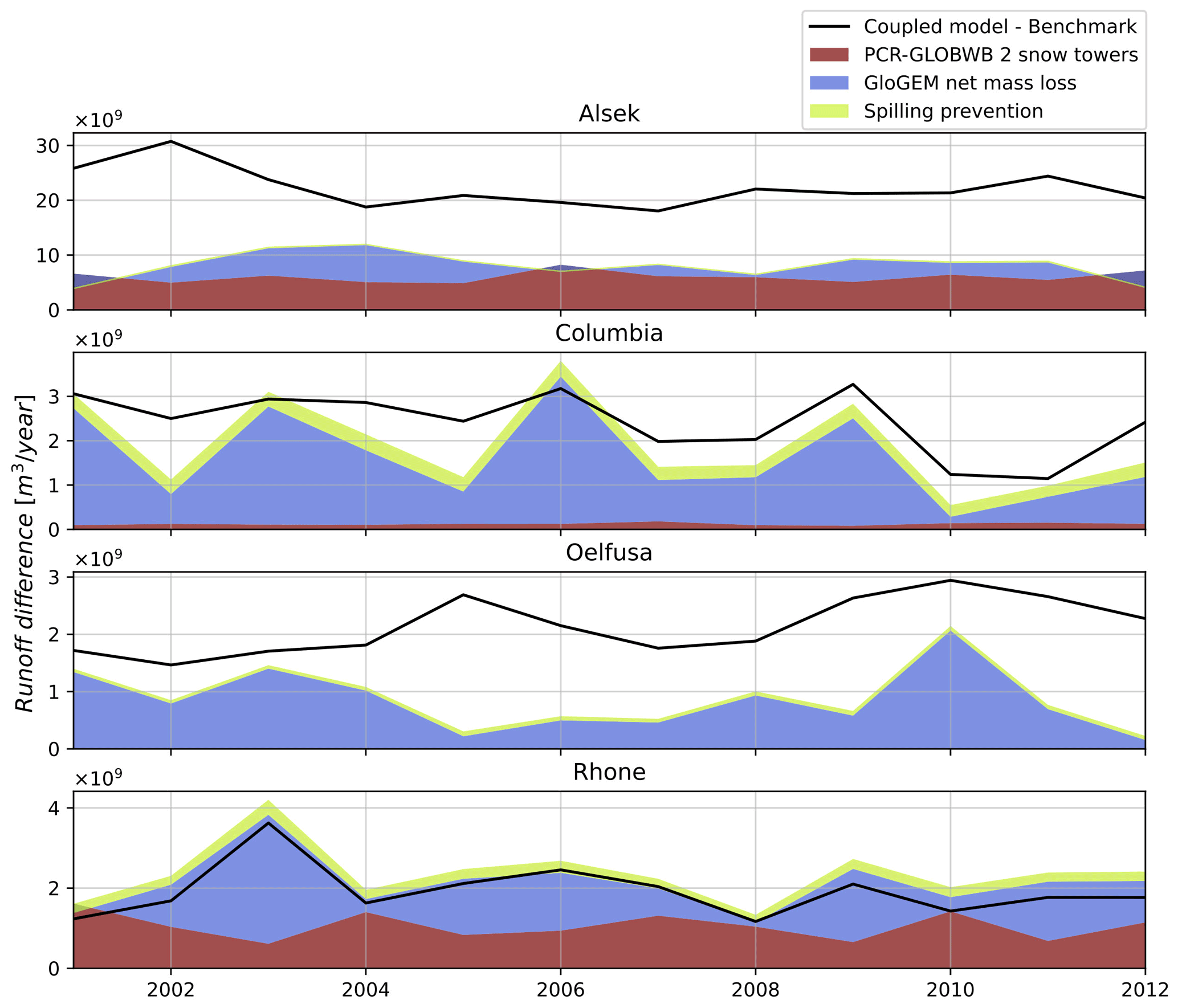
Figure 5Mechanisms explaining the runoff difference between the coupled model and the benchmark. The black line represents the difference in annual runoff sums. The gray stack represents the annual increase in the snow water equivalent modeled by PCR-GLOBWB 2 due to the lack of a snow redistribution parameterization. The blue stack represents the annual net mass loss from retreating glaciers, as modeled by GloGEM. The red stack represents the annual glacier runoff that would have spilled into neighboring basins as a consequence of basin boundary rasterization. This contributes to the imbalance, since the spilling prevention is not applied to the benchmark. Note that the dark blue parts represent annual GloGEM net mass gain.
Firstly, the lack of snow redistribution parameterization in PCR-GLOBWB 2 leads to the formation of “snow towers” (Freudiger et al., 2017). Gravitational glacier flow, wind, and avalanches are known to redistribute ice and snow from high elevations towards lower elevations, where melt is more likely to occur. Not accounting for these processes will lead to multiannual accumulation of snow at high elevations, where temperatures rarely drop below melting point. As an extreme example, in an Amazonian glacierized grid cell, this accumulation amounted up to a 4 m water equivalent per year. We should note that this snow accumulation is purely virtual and does not lead to an increase in the DEM. Out of the 25 basins, 17 simulate significant snow towers (see Fig. S5). This phenomenon is acknowledged by Sutanudjaja et al. (2018) for polar regions. By contrast, GloGEM indirectly accounts for glacier flow through a geometry change module (Huss et al., 2010), which prevents the buildup of large amounts of static snow masses and ensures the transport of snow to lower elevations, where melt is possible.
Secondly, PCR-GLOBWB 2 effectively treats glaciers as static rock masses and is therefore not able to capture changes in runoff following changes in glacier mass balance. Currently, many glaciers experience a peak in mass loss and, therefore, in glacier runoff (Huss and Hock, 2018); however, in PCR-GLOBWB 2, no mass will be lost, and therefore, no additional interannual glacier runoff will be simulated. This problem was also noted by Sutanudjaja et al. (2018) after observing a negative correlation of the simulated total water storage with gravimetry measurements in Alaskan and Icelandic basins. Meanwhile, GloGEM was specifically developed to model global glacier mass balances and their dependence on future dynamic changes in ice extent. It has been calibrated to and validated against observations of multiple sources (Gardner et al., 2013; Hugonnet et al., 2021; WGMS, 2021) and is therefore likely to provide more reliable estimates of mass change-induced glacier runoff.
Thirdly, while the spilling prevention (Sect. 3.3) may have helped in accurately routing all GloGEM glacier runoff in the coupled model, no similar measures were taken for the benchmark. Effectively, this leads to a larger basin area for the coupled model (0 %–2 % larger) and, consequently, to a greater basin runoff. This effect is greater in basins where a large portion of the glaciers is located at the basin boundary. The difference in basin runoff has been calculated for the four representative basins by performing additional coupled model runs without the spilling prevention and, consequently, by calculating the difference from the original coupled model runs. While this difference only ranged between 1.5 % and 4 % for these four basins during the melt season, it could explain as much as 22 % of the annual difference between the coupled model and the benchmark (see Columbia 2010 in Fig. 5).
The above-mentioned factors do not explain the entirety of the runoff difference between the coupled model and the benchmark. Particularly in the strongly glacier-influenced Alsek and Oelfusa basins, large gaps are left unaccounted for by the explanations above (i.e., the white space under the black lines in Fig. 5a and c). Evaporation and sublimation as well as groundwater recharge calculations are included in PCR-GLOBWB 2 and not in GloGEM. They could therefore (temporarily) account for part of the runoff difference, but their overall effect is estimated to be small. The differences can most likely be attributed almost entirely to the precipitation correction factor cprec used in GloGEM. This correction factor allows for a scaling of the re-analysis grid cell precipitation to actual accumulation on the glacier. In fact, the elevation range occupied by glaciers is always strongly underrepresented in the smoothed topography of the re-analysis, leading to an underestimation of orographically enhanced precipitation in the re-analysis product that needs to be accounted for (Immerzeel et al., 2015). Typically, re-analysis precipitation is upscaled by a factor of between 1.5 and 2.5 in order to correctly represent the observed mass flux components on glaciers (Huss and Hock, 2015; WGMS, 2021). Consequently, a higher grid cell precipitation in the coupled model is likely when it is applied without a counter-correction in PCR-GLOBWB 2. Unless the snow towers absorb this excess precipitation, it will cause a higher runoff estimate than in the benchmark (albeit with a certain time lag).
5.1.2 Late spring difference
Despite the above-mentioned mechanisms causing PCR-GLOBWB 2 to underestimate the glacier runoff, there is nonetheless a short period in late spring where the benchmark still produces slightly higher runoff than the coupled model in many basins (late May in Fig. 3a). These basins only partially overlap with the basins in which no snow towers were found and, equally, in which no correlation with geographical location or climate was discovered. We hypothesize this effect to be the result of the limited horizontal and vertical spatial resolutions of the temperature forcing in PCR-GLOBWB (Beek et al., 2011). Mountainous regions are characterized by steep horizontal and vertical temperature gradients, causing snow and glacier processes to be highly spatially dependent. If a model fails to capture these gradients due to an insufficient spatial or elevational resolution, there is a high chance of the melt being simulated too suddenly (Sexstone et al., 2020; Immerzeel et al., 2014). PCR-GLOBWB 2 does facilitate a temperature downscaling from the 45 arcmin of ERA-Interim to the 5 arcmin model resolution using lapse rates from the CRU CL 2.0 climatology (New et al., 2002) to better account for snow dynamics, but this is arguably still too coarse for the gradients present at glacierized mountain areas. Beek et al. (2011) additionally hypothesize part of the melt timing error of PCR-GLOBWB 2 to be a consequence of the use of a constant melt rate and threshold temperature in the snow module. However, it should be mentioned that the high spatial resolution needed in mountainous areas is still rather unfeasible for models that are designed to operate on a global scale, and therefore, a certain degree of simplification will always be present. One solution to partly overcome this problem would be the use of a multi-resolution grid (e.g., Marsh et al., 2018; Özgen Xian et al., 2020). GloGEM does not downscale ERA-Interim data spatially, but it applies to all glacier elevation bands a set of 12 constant monthly temperature lapse rates derived from the mean temperature in different pressure levels of the reanalysis (Huss and Hock, 2015). By covering a wider elevation range, GloGEM is likely to ensure a more gradual melt process along late spring, particularly in the high-temperature gradients around the highest elevations. In the present study, this is partly counteracted by the monthly jumps in glacier runoff owing to the temporal downscaling strategy (see Sect. 4.1), but this effect is deemed to be of minor importance.
5.2 Evaluation against observations
When using the RRD to evaluate the performance of the coupled model for reproducing observed basin runoff, there are two main reasons to attribute more importance to the results obtained for strongly glacier-influenced basins. Firstly, the quality of the glacier representation has greater implications in strongly glacier-influenced basins compared to weakly glacier-influenced basins and is therefore better reflected by the RRD. Secondly, in many weakly glacier-influenced basins, PCR-GLOBWB 2 mostly overestimates the basin runoff (e.g., Danube, Ob, Irrawaddy), even without considering any glacier runoff (i.e., the bare model). Since the coupling of GloGEM generally leads to even higher runoff, the RRD will be mostly negative in weakly glacier-influenced basins, even in the hypothetical case that the glacier runoff is simulated perfectly with the coupled model.
The majority of RRD values for strongly glacier-influenced (GC99>0.5) basins are positive: the RRD is positive for five out of nine values in May and June, seven out of nine in July and August, and two out of nine in September (Northern Hemisphere). Thus, particularly at the peak of the melt season (July and August), the coupled model performs better than the benchmark overall. The lesser performance in September can be partially explained by PCR-GLOBWB 2 reproducing the observations more closely, causing the addition of GloGEM to lead to an overestimation (e.g., Thjorsa, Alsek). The highest scores over all metrics are obtained by the basin with the highest maximum glacier contribution, the Oelfusa basin in Iceland. This is mostly explained by the heavy underestimation of the summer runoff by PCR-GLOBWB 2.
A major limitation of using runoff observations at the basin outlet is that they are not a direct measure of glacier runoff, and therefore, we can not fully exclude the possibility that GloGEM overestimates the glacier runoff and simply compensates for other deficits of PCR-GLOBWB 2 at the basin level to reach the higher RRD scores. While we chose the discharge stations as close to the glacier sink as possible, in many cases we excluded other upstream discharge stations from our analysis. Future studies are encouraged to consider multiple discharge stations per basin to limit this identifiability problem. Nonetheless, several aspects of our study point against the abovementioned possibility. Firstly, since GloGEM has been calibrated and validated with glacier mass balance observations (Gardner et al., 2013), it is unlikely that GloGEM heavily underestimates glacier runoff, at least on a monthly scale. Secondly, an indication that the PCR-GLOBWB 2 underestimation stems from glacierized areas is given by the observation at the Greater Aletsch Glacier (see Sect. S2), where PCR-GLOBWB 2 simulates zero runoff over multiple years. Finally, in Sect. 5.1, we provide evidence that the difference in glacier parameterization between PCR-GLOBWB 2 and GloGEM is responsible for a large part of the difference in runoff.
In conclusion, strongly glacier-influenced basins produce higher and more significant RRD scores at the same time, and we have shown this to be mostly attributable to the difference in glacier representation. The coupling of GloGEM is therefore likely to prevent significant underestimation of glacier runoff in PCR-GLOBWB 2. While, in this study, the coupling does not lead to better results for weakly glacier-influenced basins, it is probable that the glacier parameterization has in fact improved the resulting runoff in these basins, at least close to the headwaters, but that this is not visible in the results.
We coupled the global hydrological model PCR-GLOBWB 2 with the global glacier model GloGEM to investigate whether this coupling can lead to better GHM glacier representation and runoff predictions in glacierized basins. The coupling was performed by adding the rasterized and resampled GloGEM glacier runoff to the channel storage of the PCR-GLOBWB 2 grid cells. To avoid double counting, in each grid cell, a fraction equal to the glaciation degree was subtracted from the grassland land cover type. Both the uncoupled benchmark and the coupled model were run for 25 large-scale (>50 000 km2), glacierized basins across multiple continents during the hydrological years 2001–2012. The results were evaluated both mutually and against GRDC runoff observations. The main outcomes are the following:
-
The coupled model produces higher runoff across all basins. In July and August, this difference ranges from below 0.1 % for weakly glacier-influenced basins to more than 250 % for strongly glacier-influenced basins. The difference can be attributed mainly to an underestimation of runoff by PCR-GLOBWB 2, which simulates the formation of permanent “snow towers” and does not account for the additional melt induced by the retreat of glaciers worldwide.
-
Nonetheless, in some basins, the coupled model produces lower runoff than the benchmark in late spring, when the benchmark is likely to simulate a more abrupt onset of the melt season due to a limited spatial resolution.
-
In strongly glacier-influenced basins, where the coupling has the largest impact, the coupled model produces largely positive results in the evaluation against basin runoff observations. For weakly glacier-influenced basins, an inverse trend is often observed, which can be linked to the coupling generally exacerbating the overestimation of basin runoff by PCR-GLOBWB 2.
Combined, these outcomes suggest that the coupling of a global hydrological model and a global glacier model can lead to a better representation of glaciers and, hence, high-mountain hydrology as well as a high likelihood of increased runoff prediction quality in glacierized basins. This study underlines the importance of glacier representation in strongly glacier-influenced basins. Furthermore, it validates the feasibility of eWaterCycle II as a platform for hydrological modeling and model coupling.
Given the increased viability of global hydrological models in recent years together with their, nonetheless, limited glacier representation, there is a large potential for future research. To further test the methodology of coupling a global hydrological model with a global glacier model, future studies could apply ensembles of global hydrological and/or global glacier models, include more basins around High Mountain Asia, and/or perform a joint calibration. To facilitate such future work, we encourage future global glacier model studies to include runoff estimates in the publication of results. Alternatively, to improve the glacier representation within global hydrological models themselves, their developers could apply a multi-resolution grid and include glacier mass balance estimates and basic glacier dynamics. Ultimately, an improved glacier representation in GHMs could lead to a better understanding of the global patterns of present and future hydrology of large-scale glacierized basins.
All codes and supporting data produced for this study, as well as the results, can be found at https://doi.org/10.5281/zenodo.6386297 (Wiersma, 2022). The code and data required to run PCR-GLOBWB 2 are available through https://doi.org/10.5281/zenodo.247139 (Sutanudjaja, 2017). The eWaterCycle Python package and setup instructions can be found through https://doi.org/10.5281/zenodo.5119390 (Verhoeven et al., 2021), which also includes instructions on how to set up PCR-GLOBWB 2 within eWaterCycle and how to acquire the ERA-Interim forcing data (Dee et al., 2011). The original GloGEM glacier runoff and mass balance data, and the more recent model outputs, are available from Matthias Huss upon request. The river runoff data can be requested from the Global Runoff Data Centre (https://www.bafg.de/GRDC, GRDC, 2020), the French Hydroportail (https://hydro.eaufrance.fr/, Hydrobanque, 2020), and the Swiss Federal Office for the Environment (https://www.hydrodaten.admin.ch/de, BAFU, 2020), respectively. The Randolph Glacier Inventory 6.0 data are available after registration at https://doi.org/10.7265/4m1f-gd79 (RGI Consortium, 2017). The basin delineations of HydroSHEDS version 1 are available at https://www.hydrosheds.org/products/hydrosheds (Lehner et al., 2008).
The supplement related to this article is available online at: https://doi.org/10.5194/hess-26-5971-2022-supplement.
PW, RH, and JA conceptualized the work. PW took care of the data curation, formal analysis, project administration, visualization, and preparation of the original draft. PW, MHu, and EHS developed the methodology. ND, JA, and RH provided the resources and software. RH, JA, HZ, and MHr supervised and validated the work. All authors contributed to the review and editing of the paper.
At least one of the (co-)authors is a member of the editorial board of Hydrology and Earth System Sciences. The peer-review process was guided by an independent editor, and the authors also have no other competing interests to declare.
Publisher's note: Copernicus Publications remains neutral with regard to jurisdictional claims in published maps and institutional affiliations.
Harry Zekollari has been supported by funding received from an EU Horizon 2020 Marie Skłodowska-Curie Individual Fellowship (grant no. 799904) and from the Fonds de la Recherche Scientifique – FNRS (postdoctoral grant – chargé de recherches). Jerom Aerts and Rolf Hut have received funding from the Netherlands eScience Center (grant no. 027.017.F01).
This paper was edited by Stacey Archfield and reviewed by two anonymous referees.
Aerts, J. P. M., Uhlemann-Elmer, S., Eilander, D., and Ward, P. J.: Comparison of estimates of global flood models for flood hazard and exposed gross domestic product: a China case study, Nat. Hazards Earth Syst. Sci., 20, 3245–3260, https://doi.org/10.5194/nhess-20-3245-2020, 2020. a
Ayala, A., Pellicciotti, F., MacDonell, S., McPhee, J., and Burlando, P.: Patterns of glacier ablation across north-central chile: identifying the limits of empirical melt models under sublimation-favorable conditions: Glacier Ablation in the Semiarid Andes, Water Resour. Res., 53, 5601–5625, https://doi.org/10.1002/2016WR020126, 2017. a
BAFU: Hydrologische Daten und Vorhersagen, BAFU [data set], https://www.hydrodaten.admin.ch/de (last access: 21 September 2020), 2020. a, b
Barbarossa, V., Bosmans, J., Wanders, N., King, H., Bierkens, M. F. P., Huijbregts, M. A. J., and Schipper, A. M.: Threats of global warming to the world's freshwater fishes, Nat. Commun., 12, 1701, https://doi.org/10.1038/s41467-021-21655-w, 2021. a
Beek, L. P. H. V., Wada, Y., and Bierkens, M. F. P.: Global monthly water stress: 1. Water balance and water availability, Water Resour. Res., 47, W07517, https://doi.org/10.1029/2010wr009791, 2011. a, b, c
Bergström, S.: The HBV model, chap, 13, in: Computer Models of Watershed Hydrology, edited by: Singh, V. P., Water Resources Publications, Highlands Ranch, Colorado, USA, 443–476, ISBN 10 1887201742, ISBN 13 978-1887201742, 1995. a
Biemans, H., Siderius, C., Lutz, A. F., Nepal, S., Ahmad, B., Hassan, T., von Bloh, W., Wijngaard, R. R., Wester, P., Shrestha, A. B., and Immerzeel, W. W.: Importance of snow and glacier meltwater for agriculture on the indo-gangetic plain, Nature Sustainability, 2, 594–601, https://doi.org/10.1038/s41893-019-0305-3, 2019. a
Bliss, A., Hock, R., and Radić, V.: Global response of glacier runoff to twenty-first century climate change, J. Geophys. Res.-Earth, 119, 717–730, https://doi.org/10.1002/2013jf002931, 2014. a
Brunner, M. I., Farinotti, D., Zekollari, H., Huss, M., and Zappa, M.: Future shifts in extreme flow regimes in Alpine regions, Hydrol. Earth Syst. Sci., 23, 4471–4489, https://doi.org/10.5194/hess-23-4471-2019, 2019. a
Cáceres, D., Marzeion, B., Malles, J. H., Gutknecht, B. D., Müller Schmied, H., and Döll, P.: Assessing global water mass transfers from continents to oceans over the period 1948–2016, Hydrol. Earth Syst. Sci., 24, 4831–4851, https://doi.org/10.5194/hess-24-4831-2020, 2020. a, b, c
Castellazzi, P., Burgess, D., Rivera, A., Huang, J., Longuevergne, L., and Demuth, M. N.: Glacial melt and potential impacts on water resources in the canadian rocky mountains, Water Resour. Res., 55, 10191–10217, https://doi.org/10.1029/2018wr024295, 2019. a
Cauvy-Fraunié, S. and Dangles, O.: A global synthesis of biodiversity responses to glacier retreat, Nature Ecology & Evolution, 3, 1675–1685, https://doi.org/10.1038/s41559-019-1042-8, 2019. a
Dee, D. P., Uppala, S. M., Simmons, A. J., Berrisford, P., Poli, P., Kobayashi, S., Andrae, U., Balmaseda, M. A., Balsamo, G., Bauer, P., Bechtold, P., Beljaars, A. C. M., van de Berg, L., Bidlot, J., Bormann, N., Delsol, C., Dragani, R., Fuentes, M., Geer, A. J., Haimberger, L., Healy, S. B., Hersbach, H., Hólm, E. V., Isaksen, L., Kållberg, P., Köhler, M., Matricardi, M., Mcnally, A. P., Monge-Sanz, B. M., Morcrette, J. J., Park, B. K., Peubey, C., de Rosnay, P., Tavolato, C., Thépaut, J. N., and Vitart, F.: The ERA-interim reanalysis: configuration and performance of the data assimilation system, Q. J. Roy. Meteor. Soc., 137, 553–597, https://doi.org/10.1002/qj.828, 2011. a, b
Do, H. X., Zhao, F., Westra, S., Leonard, M., Gudmundsson, L., Boulange, J. E. S., Chang, J., Ciais, P., Gerten, D., Gosling, S. N., Müller Schmied, H., Stacke, T., Telteu, C.-E., and Wada, Y.: Historical and future changes in global flood magnitude – evidence from a model–observation investigation, Hydrol. Earth Syst. Sci., 24, 1543–1564, https://doi.org/10.5194/hess-24-1543-2020, 2020. a
Edwards, T. L., Nowicki, S., Marzeion, B., Hock, R., Goelzer, H., Seroussi, H., Jourdain, N. C., Slater, D. A., Turner, F. E., Smith, C. J., McKenna, C. M., Simon, E., Abe-Ouchi, A., Gregory, J. M., Larour, E., Lipscomb, W. H., Payne, A. J., Shepherd, A., Agosta, C., Alexander, P., Albrecht, T., Anderson, B., Asay-Davis, X., Aschwanden, A., Barthel, A., Bliss, A., Calov, R., Chambers, C., Champollion, N., Choi, Y., Cullather, R., Cuzzone, J., Dumas, C., Felikson, D., Fettweis, X., Fujita, K., Galton-Fenzi, B. K., Gladstone, R., Golledge, N. R., Greve, R., Hattermann, T., Hoffman, M. J., Humbert, A., Huss, M., Huybrechts, P., Immerzeel, W., Kleiner, T., Kraaijenbrink, P., Le clec'h, S., Lee, V., Leguy, G. R., Little, C. M., Lowry, D. P., Malles, J.-H., Martin, D. F., Maussion, F., Morlighem, M., O'Neill, J. F., Nias, I., Pattyn, F., Pelle, T., Price, S. F., Quiquet, A., Radić, V., Reese, R., Rounce, D. R., Rückamp, M., Sakai, A., Shafer, C., Schlegel, N.-J., Shannon, S., Smith, R. S., Straneo, F., Sun, S., Tarasov, L., Trusel, L. D., Van Breedam, J., van de Wal, R., van den Broeke, M., Winkelmann, R., Zekollari, H., Zhao, C., Zhang, T., and Zwinger, T.: Projected land ice contributions to twenty-first-century sea level rise, Nature, 593, 74–82, https://doi.org/10.1038/s41586-021-03302-y, 2021. a
Eyring, V., Bony, S., Meehl, G. A., Senior, C. A., Stevens, B., Stouffer, R. J., and Taylor, K. E.: Overview of the Coupled Model Intercomparison Project Phase 6 (CMIP6) experimental design and organization, Geosci. Model Dev., 9, 1937–1958, https://doi.org/10.5194/gmd-9-1937-2016, 2016. a
Farinotti, D., Usselmann, S., Huss, M., Bauder, A., and Funk, M.: Runoff evolution in the swiss alps: projections for selected high-alpine catchments based on ENSEMBLES scenarios, Hydrol. Process., 26, 1909–1924, https://doi.org/10.1002/hyp.8276, 2012. a
Frans, C., Istanbulluoglu, E., Lettenmaier, D. P., Fountain, A. G., and Riedel, J.: Glacier recession and the response of summer streamflow in the pacific northwest united states, 1960–2099, Water Resour. Res., 54, 6202–6225, https://doi.org/10.1029/2017wr021764, 2018. a
Freudiger, D., Kohn, I., Seibert, J., Stahl, K., and Weiler, M.: Snow redistribution for the hydrological modeling of alpine catchments, WIRes Water, 4, 1–16, https://doi.org/10.1002/wat2.1232, 2017. a
Gardner, A. S., Moholdt, G., Cogley, J. G., Wouters, B., Arendt, A. A., Wahr, J., Berthier, E., Hock, R., Pfeffer, W. T., Kaser, G., Ligtenberg, S. R. M., Bolch, T., Sharp, M. J., Hagen, J. O., Broeke, M. R. V. D., and Paul, F.: A reconciled estimate of glacier contributions to sea level rise: 2003 to 2009, Science, 340, 852–857, https://doi.org/10.1126/science.1234532, 2013. a, b
Gevaert, A. I., Veldkamp, T. I. E., and Ward, P. J.: The effect of climate type on timescales of drought propagation in an ensemble of global hydrological models, Hydrol. Earth Syst. Sci., 22, 4649–4665, https://doi.org/10.5194/hess-22-4649-2018, 2018. a
GRDC: The global runoff data centre, 56068 Koblenz, Germany, GRDC [data set], Germany, https://www.bafg.de/GRDC (last access: 23 November 2020), 2020. a, b
Hanus, S., Hrachowitz, M., Zekollari, H., Schoups, G., Vizcaino, M., and Kaitna, R.: Future changes in annual, seasonal and monthly runoff signatures in contrasting Alpine catchments in Austria, Hydrol. Earth Syst. Sci., 25, 3429–3453, https://doi.org/10.5194/hess-25-3429-2021, 2021. a
He, Z., Duethmann, D., and Tian, F.: A meta-analysis based review of quantifying the contributions of runoff components to streamflow in glacierized basins, J. Hydrol., 603, 126890, https://doi.org/10.1016/j.jhydrol.2021.126890, 2021. a
Hirabayashi, Y., Döll, P., and Kanae, S.: Global-scale modeling of glacier mass balances for water resources assessments: glacier mass changes between 1948 and 2006, J. Hydrol., 390, 245–256, https://doi.org/10.1016/j.jhydrol.2010.07.001, 2010. a
Hock, R., Bliss, A., Marzeion, B. E. N., Giesen, R. H., Hirabayashi, Y., Huss, M., Radic, V., and Slangen, A. B. A.: GlacierMIP-A model intercomparison of global-scale glacier mass-balance models and projections, J. Glaciol., 65, 453–467, https://doi.org/10.1017/jog.2019.22, 2019. a
Hugonnet, R., McNabb, R., Berthier, E., Menounos, B., Nuth, C., Girod, L., Farinotti, D., Huss, M., Dussaillant, I., Brun, F., and Kääb, A.: Accelerated global glacier mass loss in the early twenty-first century, Nature, 592, 726–731, https://doi.org/10.1038/s41586-021-03436-z, 2021. a, b
Huss, M.: Present and future contribution of glacier storage change to runoff from macroscale drainage basins in Europe, Water Resour. Res., 47, 1–14, https://doi.org/10.1029/2010WR010299, 2011. a
Huss, M. and Hock, R.: A new model for global glacier change and sea-level rise, Front. Earth Sci., 3, 1–22, https://doi.org/10.3389/feart.2015.00054, 2015. a, b, c, d, e
Huss, M. and Hock, R.: Global-scale hydrological response to future glacier mass loss, Nat. Clim. Change, 8, 135–140, https://doi.org/10.1038/s41558-017-0049-x, 2018. a, b, c, d, e, f, g
Huss, M., Farinotti, D., Bauder, A., and Funk, M.: Modelling runoff from highly glacierized alpine drainage basins in a changing climate, Hydrol. Process., 22, 3888–3902, https://doi.org/10.1002/hyp.7055, 2008. a
Huss, M., Jouvet, G., Farinotti, D., and Bauder, A.: Future high-mountain hydrology: a new parameterization of glacier retreat, Hydrol. Earth Syst. Sci., 14, 815–829, https://doi.org/10.5194/hess-14-815-2010, 2010. a
Hut, R., Drost, N., van de Giesen, N., van Werkhoven, B., Abdollahi, B., Aerts, J., Albers, T., Alidoost, F., Andela, B., Camphuijsen, J., Dzigan, Y., van Haren, R., Hutton, E., Kalverla, P., van Meersbergen, M., van den Oord, G., Pelupessy, I., Smeets, S., Verhoeven, S., de Vos, M., and Weel, B.: The eWaterCycle platform for open and FAIR hydrological collaboration, Geosci. Model Dev., 15, 5371–5390, https://doi.org/10.5194/gmd-15-5371-2022, 2022. a
Hutton, E., Piper, M., and Tucker, G.: The basic model interface 2.0: A standard interface for coupling numerical models in the geosciences, Journal of Open Source Software, 5, 2317, https://doi.org/10.21105/joss.02317, 2020. a
Hydrobanque: Hydrobanque, Hydrobanque [data set], https://hydro.eaufrance.fr/ (last access: 28 May 2020), 2020. a, b
Immerzeel, W. W., Petersen, L., Ragettli, S., and Pellicciotti, F.: The importance of observed gradients of air temperature and precipitation for modeling runoff from a glacierized watershed in the nepalese himalayas, Water Resour. Res., 50, 2212–2226, https://doi.org/10.1002/2013WR014506, 2014. a
Immerzeel, W. W., Wanders, N., Lutz, A. F., Shea, J. M., and Bierkens, M. F. P.: Reconciling high-altitude precipitation in the upper Indus basin with glacier mass balances and runoff, Hydrol. Earth Syst. Sci., 19, 4673–4687, https://doi.org/10.5194/hess-19-4673-2015, 2015. a
Immerzeel, W. W., Lutz, A. F., Andrade, M., Bahl, A., Biemans, H., Bolch, T., Hyde, S., Brumby, S., Davies, B. J., Elmore, A. C., Emmer, A., Feng, M., Fernández, A., Haritashya, U., Kargel, J. S., Koppes, M., Kraaijenbrink, P. D. A., Kulkarni, A. V., Mayewski, P. A., Nepal, S., Pacheco, P., Painter, T. H., Pellicciotti, F., Rajaram, H., Rupper, S., Sinisalo, A., Shrestha, A. B., Viviroli, D., Wada, Y., Xiao, C., Yao, T., and Baillie, J. E. M.: Importance and vulnerability of the world's water towers, Nature, 577, 364–369, https://doi.org/10.1038/s41586-019-1822-y, 2020. a, b, c
Jansson, P., Hock, R., and Schneider, T.: The concept of glacier storage: A review, J. Hydrol., 282, 116–129, https://doi.org/10.1016/s0022-1694(03)00258-0, 2003. a
Kaser, G., Großhauser, M., and Marzeion, B.: Contribution potential of glaciers to water availability in different climate regimes, P. Natl. Acad. Sci. USA, 107, 20223–20227, https://doi.org/10.1073/pnas.1008162107, 2010. a
Kottek, M., Grieser, J., Beck, C., Rudolf, B., and Rubel, F.: World map of the Köppen-Geiger climate classification updated, Meteorol. Z., 15, 259–263, https://doi.org/10.1127/0941-2948/2006/0130, 2006. a
Laurent, L., Buoncristiani, J. F., Pohl, B., Zekollari, H., Farinotti, D., Huss, M., Mugnier, J. L., and Pergaud, J.: The impact of climate change and glacier mass loss on the hydrology in the mont-blanc massif, Sci. Rep.-UK, 10, 1–11, https://doi.org/10.1038/s41598-020-67379-7, 2020. a
Lehner, B., Verdin, K., and Jarvis, A.: New global hydrography derived from spaceborne elevation data, Eos T. Am. Geophys. Un., 89, 93–94, https://doi.org/10.1029/2008EO100001, 2008 (data available at: https://www.hydrosheds.org/products/hydrosheds, last access: 4 June 2020). a, b, c
Marsh, C. B., Spiteri, R. J., Pomeroy, J. W., and Wheater, H. S.: Multi-objective unstructured triangular mesh generation for use in hydrological and land surface models, Comput. Geosci., 119, 49–67, https://doi.org/10.1016/j.cageo.2018.06.009, 2018. a
Marzeion, B., Jarosch, A. H., and Hofer, M.: Past and future sea-level change from the surface mass balance of glaciers, The Cryosphere, 6, 1295–1322, https://doi.org/10.5194/tc-6-1295-2012, 2012. a
Marzeion, B., Hock, R., Anderson, B., Bliss, A., Champollion, N., Fujita, K., Huss, M., Immerzeel, W. W., Kraaijenbrink, P., Malles, J. H., Maussion, F., Radić, V., Rounce, D. R., Sakai, A., Shannon, S., van de Wal, R., and Zekollari, H.: Partitioning the uncertainty of ensemble projections of global glacier mass change, Earths Future, 8, 1–25, https://doi.org/10.1029/2019ef001470, 2020. a
Maussion, F., Butenko, A., Champollion, N., Dusch, M., Eis, J., Fourteau, K., Gregor, P., Jarosch, A. H., Landmann, J., Oesterle, F., Recinos, B., Rothenpieler, T., Vlug, A., Wild, C. T., and Marzeion, B.: The Open Global Glacier Model (OGGM) v1.1, Geosci. Model Dev., 12, 909–931, https://doi.org/10.5194/gmd-12-909-2019, 2019. a
Müller Schmied, H., Cáceres, D., Eisner, S., Flörke, M., Herbert, C., Niemann, C., Peiris, T. A., Popat, E., Portmann, F. T., Reinecke, R., Schumacher, M., Shadkam, S., Telteu, C.-E., Trautmann, T., and Döll, P.: The global water resources and use model WaterGAP v2.2d: model description and evaluation, Geosci. Model Dev., 14, 1037–1079, https://doi.org/10.5194/gmd-14-1037-2021, 2021. a
Nash, J. E. and Sutcliffe, J. V.: River flow forecasting through conceptual models part I – A discussion of principles, J. Hydrol., 10, 282–290, https://doi.org/10.1016/0022-1694(70)90255-6, 1970. a
New, M., Lister, D., Hulme, M., and Makin, I.: A high-resolution data set of surface climate over global land areas, Clim. Res., 21, 1–25, https://doi.org/10.3354/cr021001, 2002. a
Özgen Xian, I., Kesserwani, G., Caviedes-Voullième, D., Molins, S., Xu, Z., Dwivedi, D., Moulton, J. D., and Steefel, C. I.: Wavelet-based local mesh refinement for rainfall–runoff simulations, J. Hydroinform., 22, 1059–1077, https://doi.org/10.2166/hydro.2020.198, 2020. a
Pfeffer, W. T., Arendt, A. A., Bliss, A., Bolch, T., Cogley, J. G., Gardner, A. S., Hagen, J. O., Hock, R., Kaser, G., Kienholz, C., Miles, E. S., Moholdt, G., Mölg, N., Paul, F., Radić, V., Rastner, P., Raup, B. H., Rich, J., Sharp, M. J., Andreassen, L. M., Bajracharya, S., Barrand, N. E., Beedle, M. J., Berthier, E., Bhambri, R., Brown, I., Burgess, D. O., Burgess, E. W., Cawkwell, F., Chinn, T., Copland, L., Cullen, N. J., Davies, B., Angelis, H. D., Fountain, A. G., Frey, H., Giffen, B. A., Glasser, N. F., Gurney, S. D., Hagg, W., Hall, D. K., Haritashya, U. K., Hartmann, G., Herreid, S., Howat, I., Jiskoot, H., Khromova, T. E., Klein, A., Kohler, J., König, M., Kriegel, D., Kutuzov, S., Lavrentiev, I., Bris, R. L., Li, X., Manley, W. F., Mayer, C., Menounos, B., Mercer, A., Mool, P., Negrete, A., Nosenko, G., Nuth, C., Osmonov, A., Pettersson, R., Racoviteanu, A., Ranzi, R., Sarikaya, M. A., Schneider, C., Sigurdsson, O., Sirguey, P., Stokes, C. R., Wheate, R., Wolken, G. J., Wu, L. Z., and Wyatt, F. R.: The randolph glacier inventory: A globally complete inventory of glaciers, J. Glaciol., 60, 537–552, https://doi.org/10.3189/2014jog13j176, 2014. a, b
Pritchard, H. D.: Asia's shrinking glaciers protect large populations from drought stress, Nature, 569, 649–654, https://doi.org/10.1038/s41586-019-1240-1, 2019. a
Radić, V. and Hock, R.: Glaciers in the earth's hydrological cycle: assessments of glacier mass and runoff changes on global and regional scales, Surv. Geophys., 35, 813–837, https://doi.org/10.1007/s10712-013-9262-y, 2014. a
Ragettli, S., Immerzeel, W. W., and Pellicciotti, F.: Contrasting climate change impact on river flows from high-altitude catchments in the himalayan and andes mountains, P. Natl. Acad. Sci. USA, 113, 9222–9227, https://doi.org/10.1073/pnas.1606526113, 2016. a
RGI Consortium: Randolph Glacier Inventory – A Dataset of Global Glacier Outlines, Version 6, RGI Consortium [data set], https://doi.org/10.7265/4m1f-gd79, 2017. a
Scanlon, B. R., Zhang, Z., Save, H., Sun, A. Y., Schmied, H. M., Van Beek, L. P., Wiese, D. N., Wada, Y., Long, D., Reedy, R. C., Longuevergne, L., Döll, P., and Bierkens, M. F.: Global models underestimate large decadal declining and rising water storage trends relative to GRACE satellite data, P. Natl. Acad. Sci. USA, 115, E1080–E1089, https://doi.org/10.1073/pnas.1704665115, 2018. a
Schaefli, B. and Gupta, H. V.: Do Nash values have value?, Hydrol. Process., 21, 2075–2080, https://doi.org/10.1002/hyp.6825, 2007. a
Schaner, N., Voisin, N., Nijssen, B., and Lettenmaier, D. P.: The contribution of glacier melt to streamflow, Environ. Res. Lett., 7, 34029, https://doi.org/10.1088/1748-9326/7/3/034029, 2012. a
Seibert, J., Vis, M. J. P., Lewis, E., and van Meerveld, H. J.: Upper and lower benchmarks in hydrological modelling, Hydrol. Process., 32, 1120–1125, https://doi.org/10.1002/hyp.11476, 2018. a
Sevestre, H. and Benn, D. I.: Climatic and geometric controls on the global distribution of surge-type glaciers: implications for a unifying model of surging, J. Glaciol., 61, 646–662, https://doi.org/10.3189/2015JoG14J136, 2015. a
Sexstone, G. A., Driscoll, J. M., Hay, L. E., Hammond, J. C., and Barnhart, T. B.: Runoff sensitivity to snow depletion curve representation within a continental scale hydrologic model, Hydrol. Process., 34, 2365–2380, https://doi.org/10.1002/hyp.13735, 2020. a
Sutanudjaja, E.: PCR-GLOBWB_model: PCR-GLOBWB version v2.1.0_beta_1, Zenodo [code], https://doi.org/10.5281/zenodo.247139, 2017. a
Sutanudjaja, E. H., van Beek, R., Wanders, N., Wada, Y., Bosmans, J. H. C., Drost, N., van der Ent, R. J., de Graaf, I. E. M., Hoch, J. M., de Jong, K., Karssenberg, D., López López, P., Peßenteiner, S., Schmitz, O., Straatsma, M. W., Vannametee, E., Wisser, D., and Bierkens, M. F. P.: PCR-GLOBWB 2: a 5 arcmin global hydrological and water resources model, Geosci. Model Dev., 11, 2429–2453, https://doi.org/10.5194/gmd-11-2429-2018, 2018. a, b, c, d, e, f
van den Oord, G., Verhoeven, S., Pelupessy, I., Aerts, J., Hut, R., van de Giesen, N., van Werkhoven, B., Weel, B., de Vos, M., Dzigan, Y., van Haren, R., van der Zwaan, J., and van Meersbergen, M.: Earth System Models as Remote Services with GRPC4BMI, Zenodo [code], https://doi.org/10.5281/zenodo.3257304, 2019. a
van Dijk, A. I. J. M., Renzullo, L. J., Wada, Y., and Tregoning, P.: A global water cycle reanalysis (2003–2012) merging satellite gravimetry and altimetry observations with a hydrological multi-model ensemble, Hydrol. Earth Syst. Sci., 18, 2955–2973, https://doi.org/10.5194/hess-18-2955-2014, 2014. a
van Tiel, M., Stahl, K., Freudiger, D., and Seibert, J.: Glacio-hydrological model calibration and evaluation, WIRes Water, 7, W07421, https://doi.org/10.1002/wat2.1483, 2020. a
Verdin, K. L. and Greenlee, S. K.: HYDRO1k documentation, Sioux Falls, ND, US Geological Survey, EROS Data Center [data set], https://doi.org/10.5066/F77P8WN0 1998. a
Verhoeven, S., Drost, N., Weel, B., Smeets, S., Kalverla, P., Alidoost, F., Vreede, B., Rolf, H., Aerts, J., and van Werkhoven, B.: eWaterCycle Python package, Zenodo [code], https://doi.org/10.5281/zenodo.5119390, 2021. a
Vincent, A., Violette, S., and Aðalgeirsdóttir, G.: Groundwater in catchments headed by temperate glaciers: A review, Earth-Sci. Rev., 188, 59–76, https://doi.org/10.1016/j.earscirev.2018.10.017, 2019. a, b, c
Wiersma, P.: Code and data to reproduce the coupling of PCR-GLOBWB 2 and GloGEM, Zenodo [code] and [data set], https://doi.org/10.5281/zenodo.6386297, 2022. a
WGMS: Fluctuations of Glaciers Database, WGMS [data set], https://doi.org/10.5904/wgms-fog-2021-05, 2021. a, b
Zekollari, H., Huss, M., and Farinotti, D.: Modelling the future evolution of glaciers in the European Alps under the EURO-CORDEX RCM ensemble, The Cryosphere, 13, 1125–1146, https://doi.org/10.5194/tc-13-1125-2019, 2019. a
Zhang, Y., Luo, Y., Sun, L., Liu, S., Chen, X., and Wang, X.: Using glacier area ratio to quantify effects of melt water on runoff, J. Hydrol., 538, 269–277, https://doi.org/10.1016/j.jhydrol.2016.04.026, 2016. a