the Creative Commons Attribution 4.0 License.
the Creative Commons Attribution 4.0 License.
 | 10 Nov 2022
On the value of satellite remote sensing to reduce uncertainties of regional simulations of the Colorado River
Mu Xiao
Zhaocheng Wang
Kristen M. Whitney
Enrique R. Vivoni
As the major water resource in the southwestern United States, the Colorado River is experiencing decreases in naturalized streamflow and is predicted to face severe challenges under future climate scenarios. To better quantify these hydroclimatic changes, it is crucial that the scientific community establishes a reasonably accurate understanding of the spatial patterns associated with the basin hydrologic response. In this study, we employed remotely sensed land surface temperature (LST) and snow cover fraction (SCF) data from the Moderate Resolution Imaging Spectroradiometer (MODIS) to assess a regional hydrological model applied over the Colorado River Basin between 2003 and 2018. Based on the comparison between simulated and observed LST and SCF spatiotemporal patterns, a stepwise strategy was implemented to enhance the model performance. Specifically, we corrected the forcing temperature data, updated the time-varying vegetation parameters, and upgraded the snow-related process physics. Simulated nighttime LST errors were mainly controlled by the forcing temperature, while updated vegetation parameters reduced errors in daytime LST. Snow-related changes produced a good spatial representation of SCF that was consistent with MODIS but degraded the overall streamflow performance. This effort highlights the value of Earth observing satellites and provides a roadmap for building confidence in the spatiotemporal simulations from regional models for assessing the sensitivity of the Colorado River to climate change.
- Article
(12270 KB) - Full-text XML
-
Supplement
(1669 KB) - BibTeX
- EndNote


Physically based numerical models of the coupled water–energy cycle have emerged as powerful tools to address critical societal needs (Fatichi et al., 2016), including flood forecasting (Maidment, 2017), irrigation operation (Gibson et al., 2017), weather and climate prediction (Baker et al., 2017; Senatore et al., 2015), and evaluations of water scarcity (Zhou et al., 2016). Over the last 3 decades, several types of hydrologic models have been developed with different levels of conceptualization that often change with the domain size due to computational constraints. One class of models, denoted as regional or macroscale models, was originally designed to serve as land surface scheme of atmospheric models and is routinely used to simulate hydrologic processes in continental basins (>105 km2) at spatial resolutions of 10 to 25 km (e.g., Lawrence et al., 2011; Liang et al., 1994; Niu et al., 2011). These processes include infiltration, evapotranspiration, runoff production, and snow accumulation and ablation that are typically simulated in a regular grid without considering lateral transfers across cells (Clark et al., 2015). In recent years, the National Water Model has combined a regional hydrologic model applied at the unprecedented resolution of 1 km with routing schemes to generate operational hydrologic predictions over the continental United States (Lahmers et al., 2019, 2021).
In many cases, hydrologic models are applied under prescribed meteorological forcings using an optimal set of parameters that are calibrated by minimizing differences between simulated streamflow and observations at one or more locations (e.g., Gou et al., 2021; Li et al., 2019; Nijssen et al., 1997; Xiao et al., 2018; Yun et al., 2020; Zhang et al., 2017). While widely used, this approach has two important limitations. First, input and structural uncertainties are often not taken into account (Gupta and Govindaraju, 2019), causing an inflation of parametric uncertainty that can exacerbate the problem of equifinality (Beven and Binley, 1992). Second, this calibration method relies only on an aggregated measure of the hydrologic response and does not consider the model's ability to capture the spatially variable internal processes (Becker et al., 2019; Ajami et al., 2004). As a result of these two limitations, this calibration approach could cause the undesirable outcome that the model provides the right answer for the wrong physical reasons (Rajib et al., 2018; Tobin and Bennett, 2017), which can in turn induce wrong conclusions when the model is applied under nonstationary conditions due to changes in land cover and/or climate.
Satellite remote sensors provide spatially distributed estimates of hydrologic states and fluxes, including soil moisture (Entekhabi et al., 2010; Njoku et al., 2003; Kerr et al., 2001), land surface temperature (LST; Shi and Bates, 2011; Wan and Dozier, 1996), snow cover fraction (SCF, Painter et al., 2009), evapotranspiration (Boschetti et al., 2019; Fisher et al., 2020), and changes in water storage (Tapley et al., 2004). These products can reduce parametric, structural, and input uncertainties in hydrologic models by including additional constraints in the calibration process (Wood et al., 2011; Fatichi et al., 2016; Ko et al., 2019). Despite this potential, the use of remote sensing products to reduce hydrologic simulation uncertainty has been explored in only a few studies. For instance, in studies by Corbari and Mancini (2014), Crow et al. (2003), and Zink et al. (2018), satellite LST was used with river discharge to calibrate model parameters, and it was found that including LST in the process improved the simulation of evapotranspiration as estimated by eddy covariance towers or other satellite products. This outcome was also found by Gutmann and Small (2010), who applied a regional model at 14 flux towers and showed that incorporating remotely sensed LST estimates in the calibration allowed the achievement of two-thirds of the improvements gained by ingesting more accurate ground LST data. In other efforts, satellite LST products have been used to verify the performance of hydrologic models, as done by Koch et al. (2016), with the North America Land Data Assimilation System (NLDAS), Xiang et al. (2014), with the TIN-based Real-time Integrated Basin Simulator (tRIBS), Xiang et al. (2017), with the Weather Research and Forecasting (WRF)-Hydro model, and Wang et al. (2021), with the Variable Infiltration Capacity (VIC) model. Finally, a few studies have enhanced streamflow simulations (Bennett et al., 2019; Bergeron et al., 2014; Tekeli et al., 2005) by improving the timing of snowmelt using remotely sensed snow cover fields.
The Colorado River basin (CRB) is a regional watershed where hydrologic simulations are needed to support short- and long-term water management decisions. Its water resources are used by almost 40 million people in seven states of southwestern U.S. (Arizona, California, Colorado, Nevada, New Mexico, Utah, and Wyoming) to irrigate ∼22 000 km2 of land and to generate over 4200 MW of hydroelectric power (USBR, 2012). The mean annual discharge of the CRB is 20.2 km3, with high interannual variability resulting from large variations in climatic forcings (Christensen et al., 2004; Gautam and Mascaro, 2018). Until 2021, the CRB was able to meet the demand of all users by storing runoff in a large system of dams, mainly operated by the U.S. Bureau of Reclamation (USBR), and transporting water through canals and aqueducts, including the Central Arizona Project. However, declines in the mean flow observed over the last 2 decades (Hoerling et al., 2019; Udall and Overpeck, 2017), combined with increasing demands, led to the first-ever declaration of water shortages in the CRB in January 2022. The water cuts affecting users in Arizona and Nevada (CAP, 2021) are expected to become more severe in the near future and impact the agricultural sector (Mitchell et al., 2022; Norton et al., 2021).
In previous studies on the hydrologic responses of the CRB using the VIC model, confidence in the model results was built mainly through comparisons against estimates of naturalized flow (e.g., Christensen et al., 2004; Vano et al., 2012, 2014; Xiao et al., 2018). The CRB is characterized by a marked difference between the colder and wetter Upper Basin, where more than 90 % of streamflow is generated (Li et al., 2017), and the warmer and drier Lower Basin, with reduced runoff production due to low precipitation, high evaporative demand, and channel transmission losses (Rajagopalan et al., 2009). As a result of this large contrast, limiting the calibration of VIC to the use of naturalized flow in the Upper Basin may lead to uncertainty in its ability to simulate the spatiotemporal hydrologic response.
The objective of this study is to improve the physical reliability of VIC simulations in the CRB by incorporating remotely sensed fields of LST and SCF obtained from the Moderate Resolution Imaging Spectroradiometer (MODIS). LST is an important variable that impacts the coupled water–energy balance, while SCF provides information on snow conditions which are crucial for quantifying runoff generation. We start from a parameterization of VIC that led to good estimates of monthly discharge in the period 2003–2018. We then apply a stepwise procedure to reduce uncertainties in model forcings, parameters, and structure based on comparisons of simulated and remotely sensed LST and SCF fields. While based on VIC, the methods proposed here can provide guidance to refine the calibration and reduce uncertainties in other physically based hydrologic models and to identify areas for structural improvement.
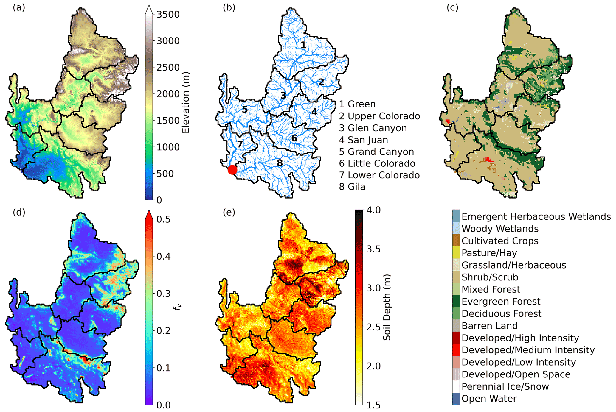
Figure 1(a) Digital elevation model of the CRB. (b) Channel network and eight subbasins analyzed in this study. The red circle marks Imperial Dam. (c) Dominant vegetation type in each pixel indicated in the legend. (d) Time-averaged vegetation fraction, fv. (e) Total soil depth. All maps are at 0.0625∘ (∼6 km) spatial resolution. Values of fv and soil depth are from the baseline simulation.
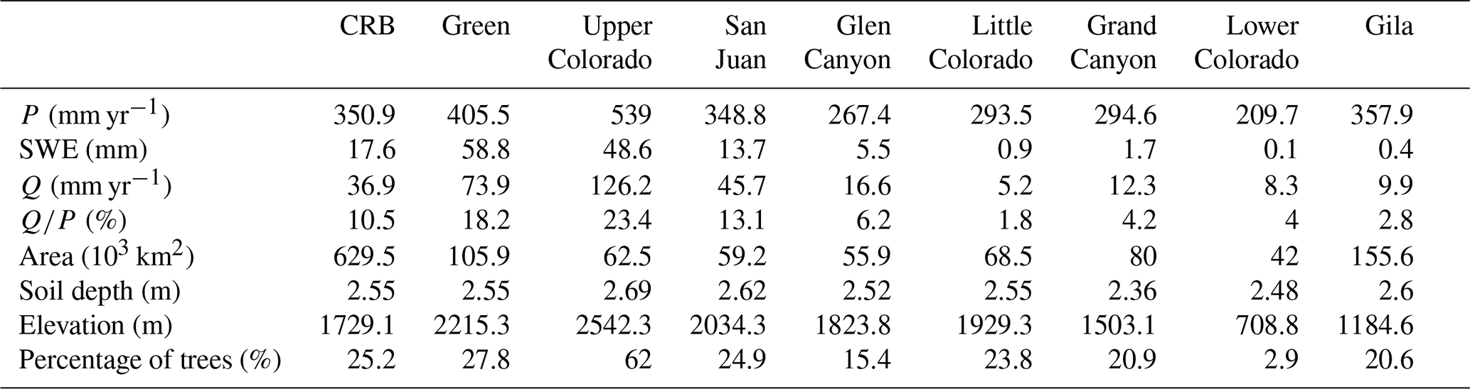
Table 1Spatially averaged mean annual precipitation (P), snow water equivalent (SWE), runoff (Q), and runoff ratio (), along with area, mean elevation, mean soil depth, and percentage of trees in the CRB and its subbasins.
2.1 Study basin
The CRB has a total area of approximately 630 000 km2, covering seven states in United States and a small portion of Mexico. Here, we considered the drainage area above Imperial Dam, plus the Gila River (Fig. 1). The Colorado River Compact of 1922 divides the CRB into the Upper and Lower basins. As revealed by the land cover map shown in Fig. 1c, most of the basin is covered by shrub or scrub ecosystems (∼60 %), followed by various forest types (∼24 %). Table 1 summarizes the mean hydroclimatic and land surface features of the subbasins. The Upper Basin consists of the Green, Upper Colorado, Glen Canyon, and San Juan River subbasins. These higher-elevation subbasins (except Glen Canyon) receive more snowfall than the rest of the CRB, resulting in the presence of a significant snowpack (mean annual snow water equivalent, or SWE, ranges from 13.7 to 58.8 mm) that eventually leads to the generation of ∼90 % of the CRB runoff. While the Lower Basin receives about 60 % of the mean annual precipitation of the subbasins in the Upper Basin per unit area, its runoff ratio (i.e., the fraction of annual precipitation becoming runoff) is 3 times smaller than that of the Upper Basin.
2.2 Remote sensing and ground-based datasets
We integrated different remotely sensed and ground-based data. Meteorological forcings were obtained from the gridded (0.0625∘ or ∼6 km) daily datasets of Livneh et al. (2013) and Su et al. (2021) for precipitation, maximum temperature, minimum temperature, and wind speed. We also used the Parameter-elevation Regressions on Independent Slopes Model (PRISM) 30-year normal (Di Luzio et al., 2008) for temperature corrections. For assessing streamflow performance, we used monthly naturalized flow records from USBR at four interior locations of the Upper Basin. Note that this is the largest available resolution for the reconstructed naturalized flow, since the river is highly regulated. To improve the simulation of spatial patterns, we used two products from the Aqua MODIS sensor, i.e., daily LST (MYD11A1) and monthly SCF (MYD10CM). The LST product is available at 1 km resolution twice a day at about 13:00 LT (local time; daytime) and 01:00 LT (nighttime; Wan et al., 2021). The percent of missing data, largely due to cloud cover, varies from 42 % to 95 %, with larger values in the winter season and July (Fig. S1 in the Supplement). Monthly SCF is provided at 0.05∘ (∼5 km) resolution as the average of SCF for days with a prescribed level of sky clearness (Hall and Riggs, 2021). Both MODIS products were aggregated to the 0.0625∘ scale used in the model. We also validated simulated and remotely sensed LST using measurements at 14 eddy covariance towers (Baldocchi et al., 2001) selected based on available data (>300 d during 2003–2018). The station locations are shown in Fig. S2, with 12 located in the Lower Basin at elevations from 987 to 2618 m. Five stations were forested, and the remaining were covered by a short canopy. We extracted records of observed longwave radiation at the stations and used them to compute LST, following Wang et al. (2021). We also used the National Land Cover Database (NLCD) Multi-Resolution Land Characteristics (MRLC) rangeland and tree canopy cover products, which contain canopy cover fraction at 30 m resolution for forests and shrublands (Homer et al., 2020).

Figure 2Schematic explaining how LST is computed in VIC (LSTV) as compared to MODIS (LSTM) in a pixel covered by short vegetation (tile A) and tall trees (tile B). fv is the vegetation fraction, Tair is the air temperature, Ts, Tf, and Tc are simulated temperatures for the surface, canopy, and canopy air, LWd,v is the downward longwave radiation from the canopy, and LWd is the downward longwave radiation from the atmosphere. The subscripts A and B refer to the variables in each tile.
3.1 The variable infiltration capacity model
We used the VIC model version 5.0 (Hamman et al., 2018) to simulate the hydrologic response of the CRB from 2003 to 2018 at an hourly time step and 0.0625∘ resolution. VIC is a macroscale, physically based model that solves the water and energy balance on a regular grid. Land surface heterogeneity in each cell is modeled through land cover tiles, each with a single vegetation class on top of a three-layer soil column. The model requires meteorological forcings as inputs and returns outputs over the grid. Fluxes and state variables simulated at grid cells are calculated as the areal-weighted average of separate computations of the water and energy balances for each land cover tile. Here, we adopted the VIC version with the clumped vegetation scheme proposed by Bohn and Vivoni (2016), where the vegetation fraction (fv) accounts for spacing between plants in each tile. This modification allows simulating the energy balance with a higher fidelity, as shown by Bohn and Vivoni (2016), through the comparison with ground estimates of evapotranspiration in the southwestern U.S. and northwestern Mexico.
Table 2List of spatially variable forcings, vegetation and soil parameters, and state variables involved in the computation of the energy balance (symbols defined in the main text and Appendix A). Forcings and state variables vary each hour. Parameters are either constant in time or vary each month (denoted with an asterisk*).

Since our adjustment strategy is based on the comparison of simulated and remotely sensed LST and SCF, we describe how these variables are simulated using the schematic in Fig. 2. The governing equations are reported in Appendix A, while the most influential parameters are in Table 2. In our simulations, 16 vegetation classes are used, which include four types of tall trees, namely deciduous forest, evergreen forest, mixed forest, and woody wetlands. For other canopy types (e.g., tile A in Fig. 2), the energy balance is solved over a control volume that combines the fractions of vegetation (fv,A) and bare soil () using a weighted aerodynamic resistance. A single surface temperature (Ts,A) is computed and assumed to be uniform over the tile and equal to the foliage temperature (). For tall trees (e.g., tile B in Fig. 2), a vegetated overstory and an understory without vegetation are introduced. If snow is absent, the overstory foliage temperature is assumed equal to air temperature (), and a single Ts,B in the understory is calculated with the scheme described above. When snow is present, Ts,B is calculated by solving the energy balance in the overstory, understory, and the atmosphere surrounding the canopy. Since the satellite sensor observes the top of the surface, the simulated LST by VIC (LSTV) that is compared against MODIS (LSTM) is the weighted average of foliage temperature in tiles with tall trees and the ground temperature in other tiles. In the case of Fig. 2, this leads to the following:
where AA and AB are the areas of tiles A and B, respectively.
To compute SCF in the grid cells, VIC allows the subdivision of each tile into elevation bands to capture changes in forcing temperature due to terrain heterogeneity. Elevation bands are the same for all tiles in a grid cell and limited typically to three bands in total. Given the mean elevation of each elevation band, the air temperature forcing is adjusted using a lapse rate of −6.5 ∘C km−1 and is then used to solve the energy balance within each tile. Depending on temperature and precipitation, snow may be simulated within a tile, and SWE is calculated. When SWE > 0, SCF is assumed to be 100 %, such that a tile within that elevation band is fully covered with snow; otherwise, SCF is 0, and the elevation band within the tile is snow-free (i.e., a binary outcome). SCF in the grid cell is the area-weighted average of the SCFs from all tiles and elevation bands.
3.2 Baseline simulation
We created a first model parameterization, labeled as baseline, based on applications by Xiao et al. (2018) and Bohn and Vivoni (2019). Hourly gridded meteorological forcings were generated from the daily grids of Livneh et al. (2013) and Su et al. (2021), using MetSim (Bennett et al., 2020; Bohn et al., 2013; Bohn and Vivoni, 2019). Model parameters were obtained from Livneh et al. (2015), with a few updates as follows. Land surface parameters were based on MODIS and NLCD products from Bohn and Vivoni (2019), which include a land cover classification and climatological monthly means of leaf area index (LAI), fv, and albedo. We replaced the elevation data used in prior VIC studies with the 30 m United States Geological Survey (USGS) National Elevation Dataset (USGS, 2017). The model was tested against monthly naturalized streamflow records, by manually adjusting seven soil parameters that affect runoff production and the parameters controlling the relation between snow albedo with snow age. As shown in Fig. S3, under the baseline simulation, VIC captured the monthly streamflow in key subbasins of the Upper Basin, where most runoff is produced, and at the basin outlet well with a Nash–Sutcliffe efficiency (NSE) > 0.9.
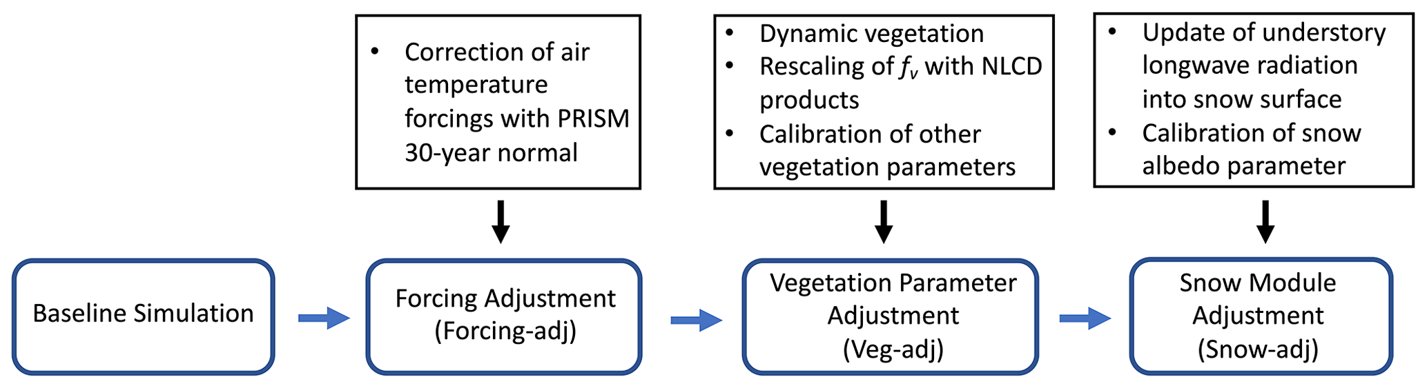
3.3 Model improvements with remote sensing products: overview of the stepwise calibration strategy
The baseline simulation was aimed at reproducing the streamflow response and did not consider the model's ability to capture spatial patterns of hydrologic variables. We designed a stepwise strategy aimed at reducing the three main sources of uncertainty in the simulation of LST and SCF. A schematic of the procedure is reported in Fig. 3; here, we provide an overview of the steps and describe the details of each step in the corresponding sections in Sect. 4. In the first step (“Forcing-adj” or forcing adjustment), we targeted input uncertainty and modified air temperature to reduce errors in nighttime LST. In the second step (“Veg-adj” or vegetation adjustment), we focused on modifying spatially variable vegetation parameters affecting daytime LST identified among those reported in Table 2. The first two steps were guided by metrics quantifying the agreement between simulated and remotely sensed LST, including the correlation coefficient (CC), root mean squared error (RMSE), and bias (mean LSTV–mean LSTM) between the (1) time series of daily LSTV and LSTM at each grid cell and (2) daily spatial maps. These metrics were obtained for both daytime and nighttime through comparisons at the MODIS overpass time. To further quantify the improvements in our calibration approach, for each step we computed the structural similarity index measure (SSIM; Wang and Bovik, 2002) and the SPAtial EFficiency (SPAEF) metric (Koch et al., 2018) between spatial maps of observed and simulated long-term climatological mean LST; these two metrics were chosen since they have been specifically designed to compare spatial patterns.
After improving LST, we reduced structural uncertainty by modifying the computation of the snow energy balance in a step labeled as “Snow-adj” (or snow adjustment). As described above, when snow exists in tiles covered by tall trees, the downward longwave radiation into the understory (or ground) snowpack is assumed to originate from the overstory (indicated as LWd,v in Fig. 2; tile B). For areas without tall trees, the downward longwave radiation reaching the understory comes from the atmosphere (indicated as LWd). To account for this in the clumped canopy scheme, we modified the downward longwave radiation as the weighted average of []. In addition, we adjusted the empirical relation controlling the change in albedo during snowmelt to reduce the bias between VIC and MODIS SCF. All modifications of the model parameters were performed via manual tuning.
4.1 Comparison of VIC and MODIS LST with ground observations
First, we provide an overview of the comparison among the time series of LST that were (1) observed at the 14 eddy covariance stations, (2) simulated by VIC, and (3) retrieved from MODIS at the co-located 6 km pixel. The error metrics for the 14 stations are summarized through box plots in Fig. 4a–c, while the time series of LST at a representative site for daytime and nighttime are shown in Fig. 4d and e. Station values and VIC simulations at the overpass times were extracted for comparison with MODIS. Dates with missing data in MODIS and station records were not considered. We find MODIS LST to be very strongly correlated with ground measurements (CC > 0.91) and characterized by RMSE from ∼1.5 to 5.3 ∘C. Bias is slightly positive (negative) during the daytime (nighttime), with a median of 0.3 ∘C (−1.6 ∘C). The error metrics for VIC reveal that performance degrades moderately with larger variability across the stations, where CC ranges from 0.70 to 0.95, the median RMSE is 6.3 ∘C (5.8 ∘C) for daytime (nighttime), and the median bias is 1.1 ∘C (−3.3 ∘C) for daytime (nighttime). The error metrics against ground data provide a reference for evaluating the model improvements, as discussed next.

Figure 4(a–c) Box plots of CC, RMSE, and bias comparing VIC and MODIS LST to observations at 14 sites. Time series of daytime (d) and nighttime LST (e) at one site (station ID “FuF”, whose location is shown in Fig. S2).
4.2 Errors in the simulation of LST in the baseline simulation and their controls
Figure 5 shows maps of CC, RMSE, and bias of the time series of LSTV and LSTM at each pixel for daytime and nighttime periods over the entire simulation from 2003 to 2018. To help the interpretation, box plots of the metrics in the grid cells within the CRB and three subbasins are presented in Fig. 6. Results for other subbasins are reported in Figs. S4–S6 and Table S1 in the Supplement.
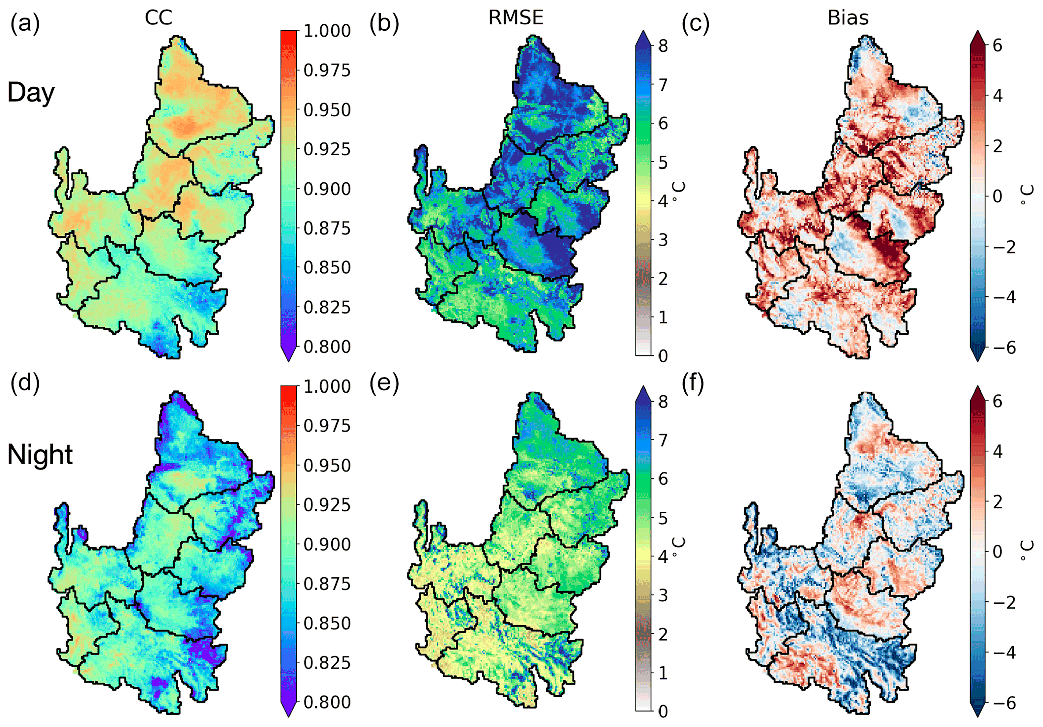
Figure 5Spatial maps of (a, d) CC, (b, e) RMSE, and (c, f) bias between time series of LSTV and LSTM over 2003–2018 at each pixel. The top (bottom) row presents daytime (nighttime) comparisons.
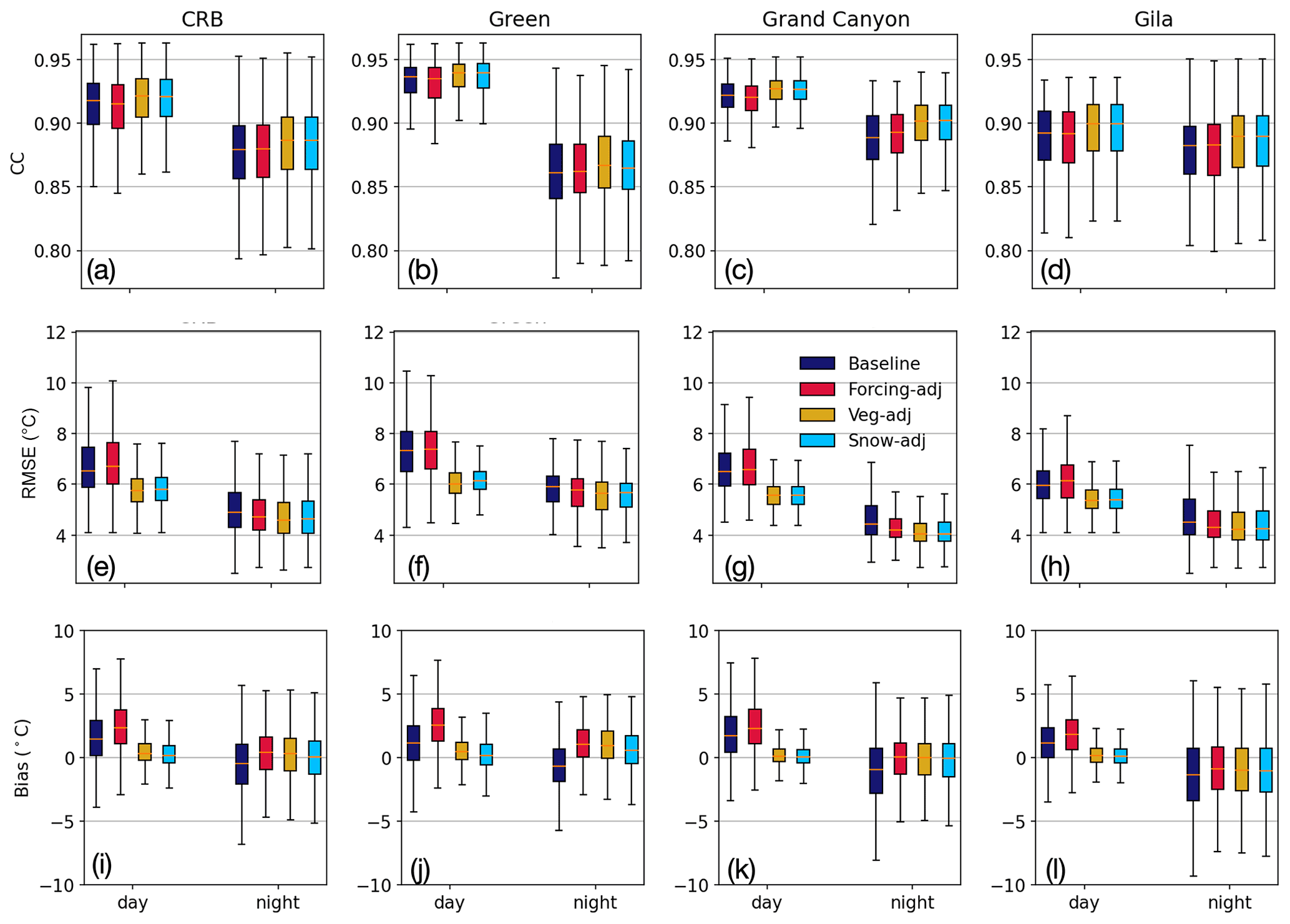
Figure 6Box plots of (a–d) CC, (e–h) RMSE, and (i–l) bias between time series of LSTV and LSTM in pixels of the entire CRB and of three representative subbasins. Box plots show the median, with 50 % and 90 % confidence intervals. Different simulations are plotted in different colors.
Overall, CC is high (>0.8) throughout the CRB, with values like those found against station data. CC is relatively higher for daytime than nighttime. On the other hand, RMSE maps show that simulated LST matches better with MODIS during the nighttime, with values largely consistent with those found for stations. For both times of the day, RMSE is slightly larger in the Upper Basin. Results for RMSE suggest that model performance for LST is relatively better at nighttime without solar radiation forcing and tends to be better in drier and hotter regions in the Lower Basin. Bias maps reveal that simulations of LST during daytime (nighttime) are warmer (cooler) than MODIS observations in most of the CRB, with a median bias of 1.2 ∘C (−0.7 ∘C). These findings are largely consistent across the subbasins and with the station observations.
Spatial patterns of the metrics are complex, suggesting that LST simulation errors are impacted by several model parameters and forcings. To gain insights into these controls, we computed the correlation coefficient between the maps of error metrics between the time series and key parameters or forcings involved in the energy balance. Model parameter maps were created by calculating the area-weighted averages within each grid cell. For monthly LAI, albedo, and fv, we computed the annual mean map. For Tair, we calculated the mean across the entire study period. Figure 7 summarizes the results in each subbasin for RMSE and bias using heatmaps (also see Fig. S7 for CC). For daytime LST, the key factors change across the subbasins, while results are more spatially uniform for nighttime LST. During daytime, we found that the Green and Upper Colorado subbasins dominated by snow and evergreen forests exhibit different controls compared to the other subbasins. Here, RMSE is highly correlated to fv and LAI, while bias is mainly controlled by Tair. In the other subbasins, albedo and, to a lesser extent, Tair are the dominant factors related to daytime RMSE. Different parameters affect the patterns of bias, including albedo in all subbasins, most vegetation parameters, root depth in the San Juan and Little Colorado, and Tair in the Little Colorado. Considering nighttime LST, Tair and, to a lower degree, soil depth are the main factors related to RMSE at all sites. Interestingly, nearly all parameters and Tair are linked to nighttime bias. This is explained by considering that Tair is correlated with elevation, and elevation is correlated with all other parameters (Fig. S8).
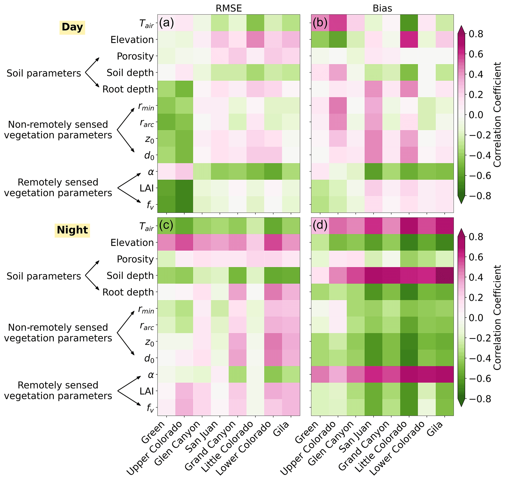
Figure 7Heatmaps showing the Pearson correlation coefficient between (1) the spatial map of Tair or key soil and vegetation parameters involved in the energy balance and (2) the spatial map of the error metrics – (a, c) RMSE and (b, d) bias – between the time series of LSTM and LSTV for the baseline simulation. The correlation coefficients are computed for each subbasin. Symbols are explained in Table 2. Top (bottom) row is for daytime (nighttime) LST.
Figure 8 presents the intra-annual variability in the error metrics between daily pairs of LSTV vs. LSTM fields, shown as monthly averages. As found previously, CC is high for both times of the day and relatively higher for daytime, while RMSE is larger during the daytime. VIC simulations during the daytime are positively biased throughout the year, while bias changes sign for nighttime LST, being positive in winter and negative from April to July. In addition, both the RMSE and bias of daytime LST are higher from April to July. This indicates that simulated daytime LST degrades when incoming solar radiation is high, especially during snowmelt events after peak SWE, typically around the end of March. To corroborate this, we repeated the analyses in snow-dominated grid cells (mean annual maximum SWE > 30 mm) and for all other cells, finding higher daytime RMSE in April for snow-dominated cells than other cells, indicating that the LST during the ablation process is also more difficult to capture.
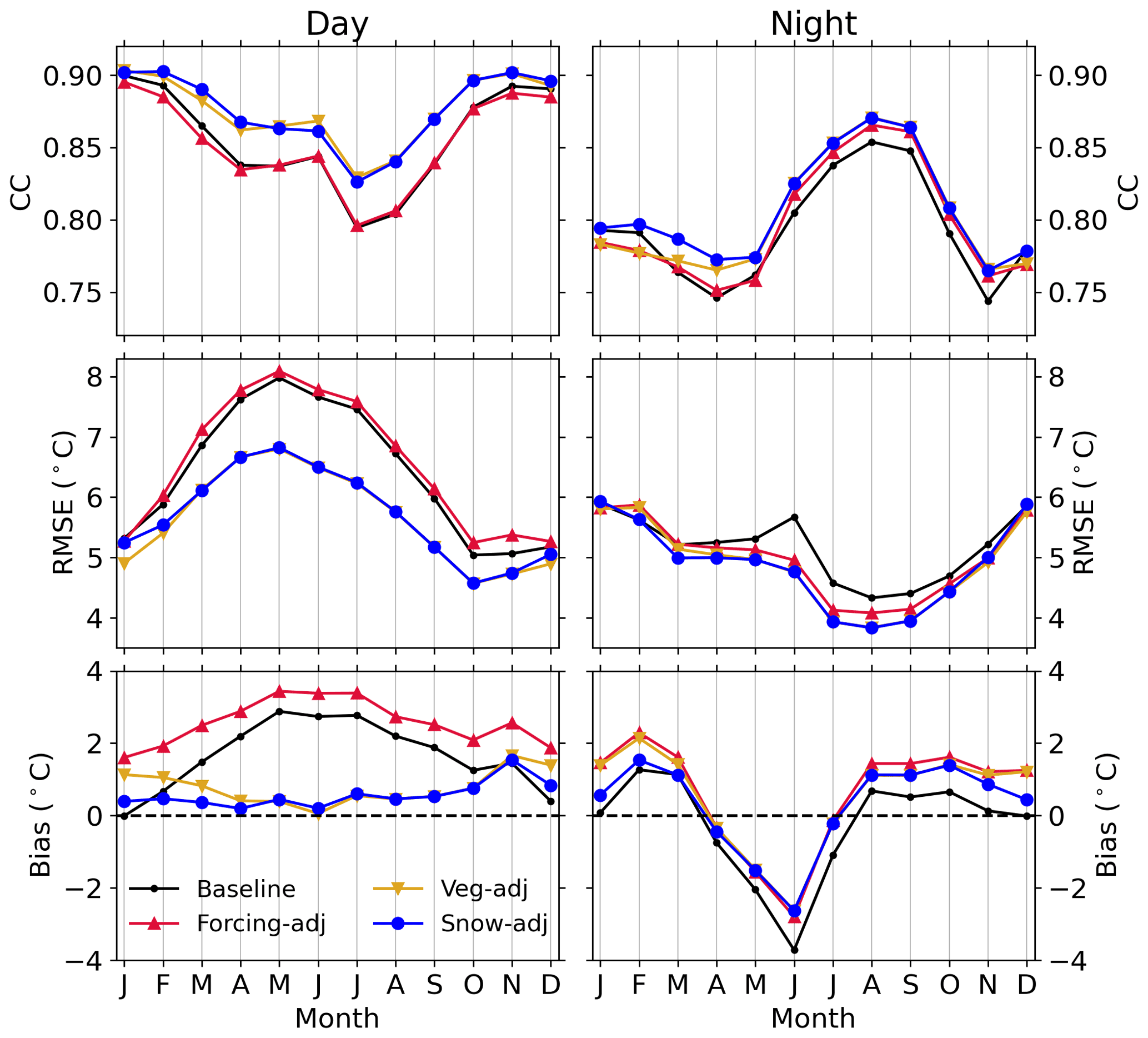
Figure 8Time series of multiyear monthly average CC, RMSE, and bias between VIC and MODIS daily LST fields for the baseline simulation and each adjustment step.
4.3 Stepwise reduction in uncertainty in the simulation of LST and SCF
4.3.1 Forcing adjustment
We first focused on the improvement in simulated LST at nighttime. Figure 7 indicates that Tair is a key input affecting the energy balance at nighttime. Alder and Hostetler (2019) compared two air temperature datasets, finding that Livneh et al. (2013) products tend to be colder than PRISM in the mountain areas of the CRB. Based on this, we adjusted the daily minimum and maximum Tair in Livneh et al. (2013) and Su et al. (2021) to match the climatological (1981–2010) monthly means from PRISM. If is the maximum or minimum daily Tair on day d and month m, then the bias-corrected value, , was obtained as follows:
where and are the climatological monthly means of maximum or minimum Tair from PRISM and Livneh et al. (2013), respectively. Once we bias-corrected Tair, we regenerated the hourly forcings using MetSim. As shown in Fig. 9, the Forcing-adj simulations improved bias, which was reduced in most subbasins. The nighttime RMSE also slightly decreased throughout the basin. These outcomes are reflected in the time series of Fig. 8 that also show that improvements (lower RMSE and bias) occur largely in the warm season. On the other hand, the Forcing-adj simulations did not improve VIC performance during the daytime, only yielding a slight increase in bias (Figs. 6 and 8) that was fixed in the next steps.
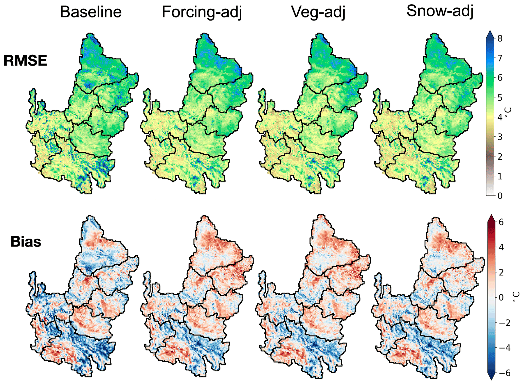
Figure 9Spatial maps of the RMSE and bias between time series of nighttime LSTV and LSTM during 2003–2018 at each pixel for all steps. Top (bottom) row presents results of RMSE (bias).
4.3.2 Vegetation parameter adjustment
Figure 7 shows that both static and time-varying vegetation parameters affect the error metrics of LST. In the Veg-adj step, we modified a set of influential parameters by incorporating new datasets. We first replaced the climatological mean monthly values of LAI, albedo, and fv with yearly varying monthly estimates from MODIS. Second, we updated fv using new products from MRLC. In the baseline simulation, fv was derived from the normalized difference vegetation index (NDVI) retrieved from MODIS (Bohn and Vivoni, 2016, 2019). MRLC released 30 m grids of mean annual fv for major vegetation types in the CRB that were used to linearly rescale values of fv in the shrub and trees classes to match the annual climatology of MRLC as follows:
where is fv in month m used in the baseline simulation, is the rescaled value, and and are long-term mean annual values of MRLC and the baseline parameters.
Figure 7 indicates that rmin, rarc, d0, and z0 affect errors in the simulation of LST, especially in the Green and Upper Colorado subbasins. Distributed estimates for these parameters are not currently available. Thus, we adjusted their values to reduce the bias between daytime LSTV and LSTM, guided by the process equations reported in Appendix A. Reducing z0 and d0 leads to lower aerodynamic resistance and higher sensible heat flux and, in turn, lower LSTV. Increases in rmin and rarc lead to lower values of latent heat flux and higher LSTV. Adjusting z0 has a greater impact than modifying the other parameters, such that the iteratively scaling of z0 in each pixel was performed at 25 %, 50 %, 150 %, or 250 %, depending on the daytime LST bias (Fig. 10). Changes were limited within physically plausible ranges. Next, we applied the same method to update d0, rmin, and rarc, but variations for these three parameters were minimal, as documented in Fig. S9.
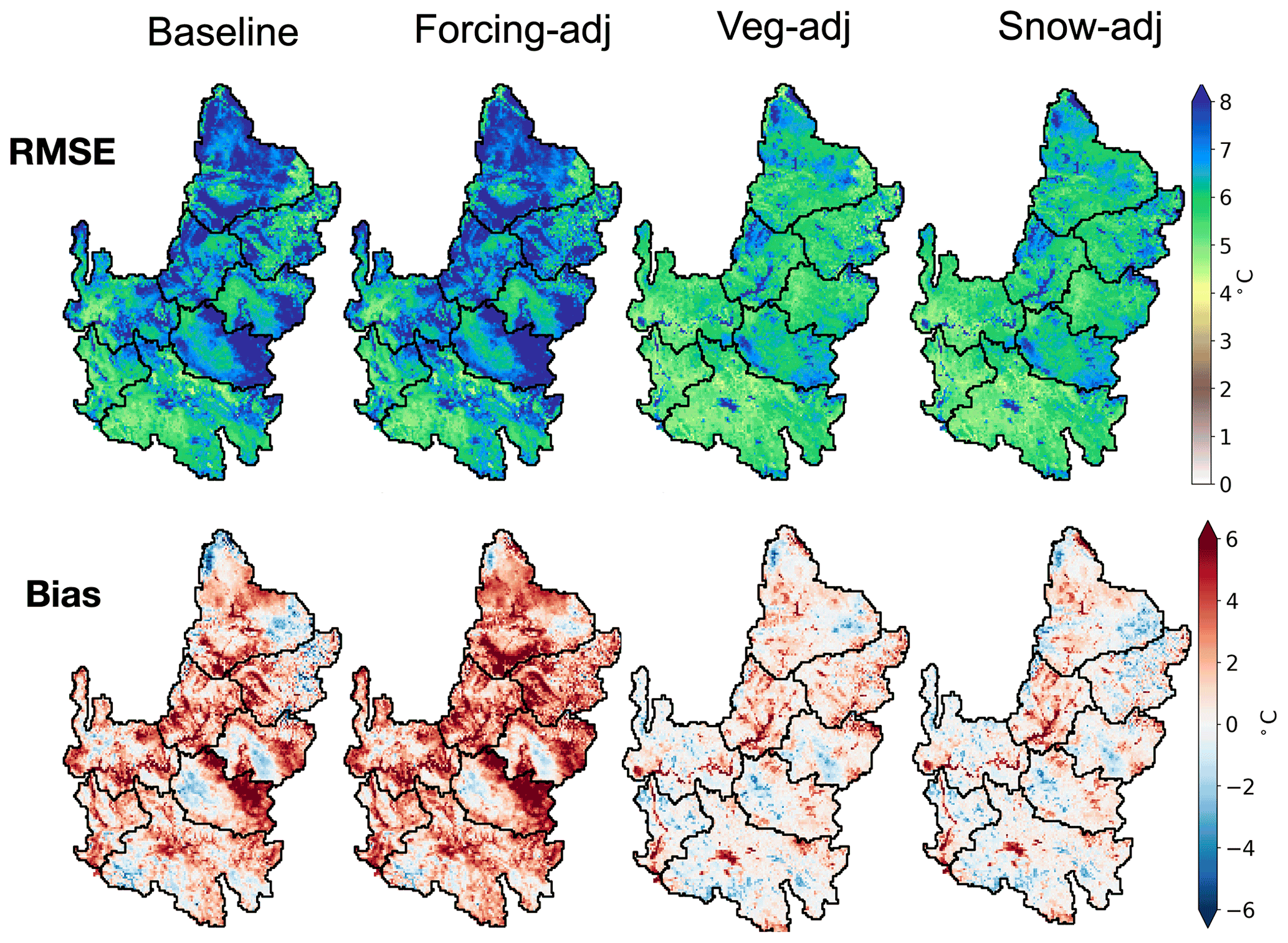
Figure 10Same as Fig. 9 but for daytime LST.
The Veg-adj simulation did not lead to significant changes in model performance at nighttime, confirming that the dominating factor affecting nighttime LST was Tair. On the other hand, improvements in the simulation of daytime LST were remarkable. Figure 6 shows that both RMSE and bias were reduced at all locations, both in terms of the median (∼0.9 ∘C) and variability in each subbasin (lower width of the confidence intervals), with values slightly higher than those found between MODIS and station observations (Fig. 4). These improvements were even more apparent in the maps of Fig. 10, which also showed that the complex spatial patterns of the errors in the baseline simulation have been replaced by more uniform and smoother patterns. The Veg-adj simulation also decreased large errors in the simulation of daytime LST from April to July, with lower RMSE, higher CC, and bias close to 0 ∘C throughout the year (Fig. 8).
4.3.3 Adjustment of snow dynamics
The Snow-adj step was aimed at improving the simulation of SCF. We first modified the computation of longwave radiation for tall trees, which improved the simulation of SCF during the snow accumulation season. Next, a parameter of the relation controlling the decay of snow albedo was modified from 0.92 to 0.80, leading to an enhanced simulation of SCF in the ablation season. Figure 11 presents bias maps between simulated and observed mean monthly SCF and seasonality of SCF in snow-dominated cells for the baseline, Veg-adj, and Snow-adj simulations. Time series of SCF in 2 pixels are also shown to visualize differences in regions with positive and negative bias. In the baseline simulation, SCF bias was positive, which occurs mainly during May through October. Forcing corrections reduced SCF, as Tair was increased in mountainous areas. Adjustments in the Snow-adj step reduced bias in most locations during the accumulation and ablation seasons. When averaged over time and in the CRB, SCF bias was relatively small. When focusing on single pixels, however, the bias magnitude was larger, with differences in seasonality depending on location. For example, bias reached +20 % (Fig. 11c) from April to December and −20 % (Fig. 11d) from November to March. As expected, Snow-adj changes mainly impacted LST simulations in mountains, while a marginal influence occurred in the rest of the CRB. Overall, the daytime LST bias map improved, while RMSE in mountain regions for both daytime and nighttime remained similar. To complete the model performance assessment, we reported, in Figs. S10 and S11, the maps of simulated and observed long-term climatology of monthly SCF in the snow season and LST, respectively, over 2003–2018. Error metrics between the maps are presented in Table S2, which shows that the overall trend of the metrics specifically designed to compare spatial patterns, SSIM and SPAEF, are in line with the changes in RMSE and bias that have been used in the rest of the paper.
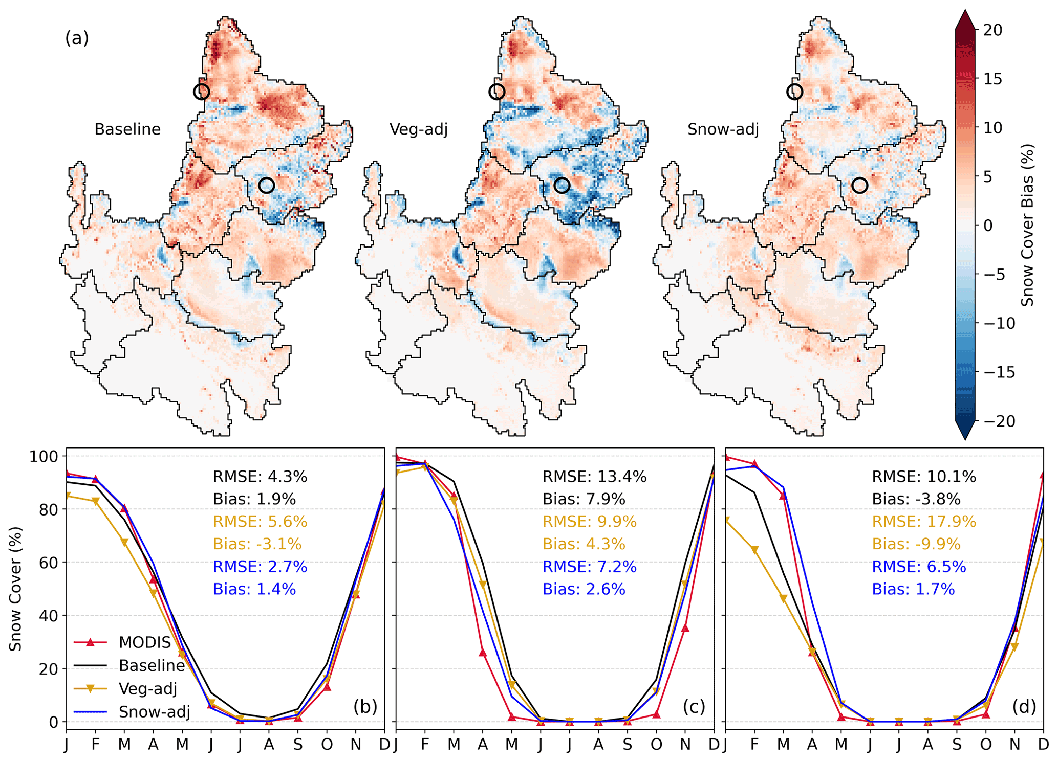
Figure 11(a) Spatial maps of bias between mean monthly SCF (VIC minus MODIS). Circles indicate the locations of two grid cells with positive and negative bias. (b) Time series of multiyear mean monthly SCF (in %) for snow-dominated cells. RMSE and bias from monthly SCF comparisons are reported. (c, d) Same as panel (b) but for sites with positive and negative bias, respectively.

Figure 12Monthly time series of naturalized streamflow (NFL) and streamflow from baseline, Forcing-adj, Veg-adj, and Snow-adj simulations at (a) Green, (b) Upper Colorado, (c) San Juan, and (d) Upper Basin for 2003–2013. NSE values are also reported.
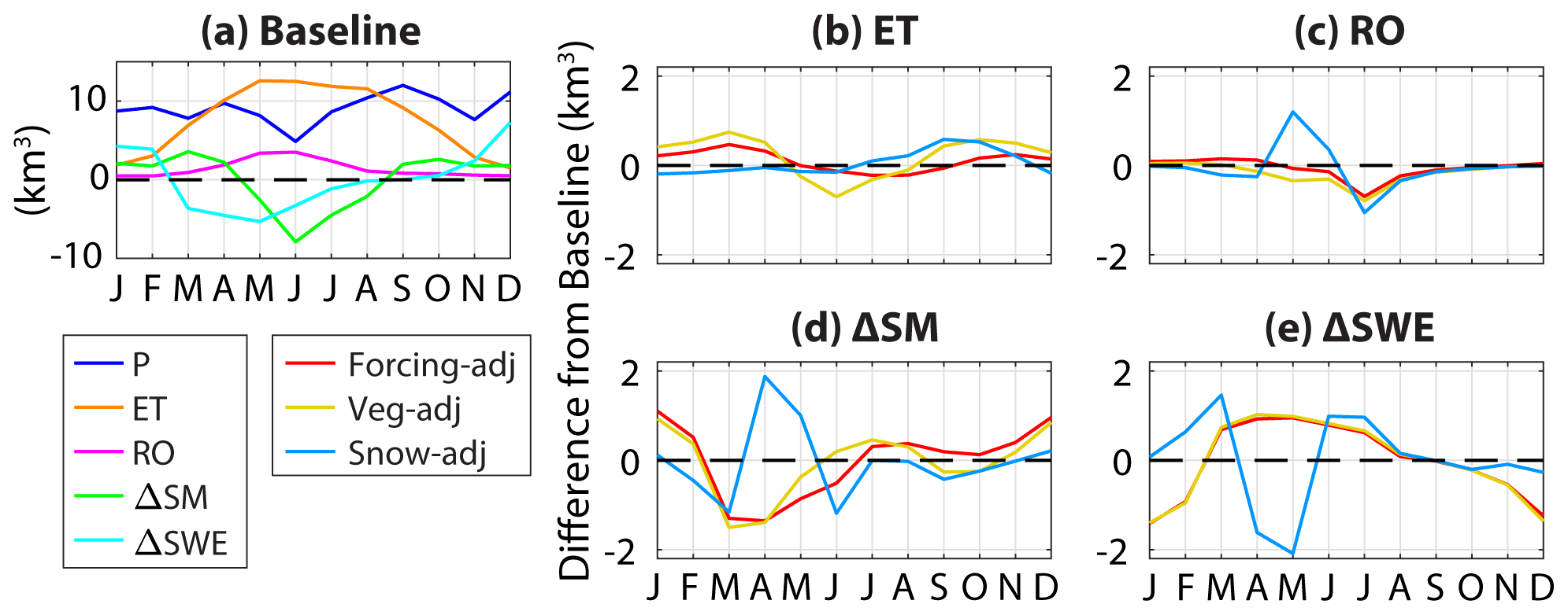
Figure 13(a) Climatological monthly mean of the water balance components for the baseline simulations in the Upper Basin. P is precipitation, ET is evapotranspiration and sublimation, RO is surface and underground runoff, and ΔSM (ΔSWE) is the differences between soil moisture (snow water equivalent) at the end and beginning of the month. (b–e) Difference between each variable for the Forcing-adj, Veg-adj, and Snow-adj simulations and the baseline simulations.
4.4 Impacts on VIC streamflow performance and water balance
As shown previously (Corbari and Mancini, 2014; Crow et al., 2003), improving the simulation of hydrologic spatial patterns could affect streamflow performance since structural limitations and different degrees of conceptualization require further tuning. We investigated this in Fig. 12, using time series of monthly runoff in the Green and San Juan subbasins and the Upper Basin. Model performance is very good for baseline simulations, since its calibration was tailored to naturalized streamflow records. Forcing and vegetation parameter adjustments slightly lowered performance (changes in NSE ≤ 0.05), whereas changes for the snow adjustment led to streamflow overestimation in May in all subbasins, especially in the Green subbasin (NSE reduced to 0.57). Overall, simulated streamflow performance here is consistent with Tang and Lettenmaier (2010), who found that incorporating MODIS snow cover degrades streamflow metrics. We attribute this degradation in performance to a number of reasons. First, remotely sensed spatiotemporal data of SCF have limitations in its usefulness for tracking SWE, which is the modeled state variable more directly impacting streamflow. Second, VIC uses a binary scheme for depicting SCF in elevation bands within each time of each grid cell, limiting its accuracy in representing topographic variations. To address these limitations, enhancements are needed in both the 1simulation of snow physics and remote sensing of the spatial variation in snow depth or SWE at high spatiotemporal resolutions.
In addition to streamflow, we explored the impacts of each calibration step on the water balance. For this aim, we computed the climatological monthly mean of the water balance components for the Upper Basin, where most runoff is generated. Results are presented in Fig. 13, which shows fluxes (P, ET, and RO; see the Fig. 13a caption for their definition) and changes in state variables (ΔSM and ΔSWE) for the baseline simulations (Fig. 13a) and the difference between a given variable simulated in each calibration step and the variable from the baseline simulation (Fig. 13b–d). The Forcing-adj and Veg-adj steps lead to small changes in ET and RO, with a decrease in both fluxes in the summer months and an increase in the other months. The modification of these fluxes is due to a change in the storage components, with (1) lower SWE (i.e., negative ΔSWE) and higher SM from November to February and (2) higher SWE and lower SM from March to July. The Snow-adj step modifies the seasonality of SWE compared to the baseline by increasing this storage component in February and March and reducing it in April and May. This, in turn, leads to an opposite behavior for SM, which is ultimately translated into a positive (negative) change in RO in May and June (July and August). In all cases, the changes in runoff occurred in a similar way for both the surface and underground components.
In this study, we made improvement to a regional hydrologic model in the Colorado River basin using MODIS observations of land surface temperature and snow cover. Based on the remotely sensed data, we corrected the meteorological forcings, updated the vegetation parameters, and revised snow-related processes to enhance the model performance. The adjustments increased the consistency between VIC and MODIS LST and SCF fields, thus enhancing credibility of the spatial simulations. Our conclusions are summarized as follows:
-
MODIS products provided spatiotemporal information that can be used to identify uncertainties in a hydrologic model calibrated with streamflow records at a few locations. Although baseline simulation performance for LST was high (mostly CC > 0.8), spatial errors within the CRB were non-negligible. The baseline simulation had lower RMSE of LST for nighttime and cold season conditions. Baseline model discrepancies were primarily associated with energy exchanges at land surface during periods of higher solar radiation.
-
Simulated nighttime LST values were dominated by the initial air temperature, such that improvements were obtained from forcing corrections. This led to a reduction in nighttime LST bias from −7 to 6 ∘C in the baseline case to −5 to 5 ∘C in the Forcing-adj simulation. Vegetation adjustments led to large improvements in daytime LST, with RMSE reductions from 7.5 to 2.5 ∘C, but were less effective at night. In addition, the range of daytime RMSE of LST was reduced from 4 to 10 ∘C in the baseline case to 2.5 to 3.5 ∘C in the Veg-adj simulation.
-
Updated snow physics reduced the negative bias in SCF during the accumulation season. We further adjusted melting snow albedo to improve performance in the ablation period. Unlike other modifications, runoff was substantially impacted by the lower snow albedo. Thus, the consistency between VIC and MODIS snow cover did not ensure an improved streamflow simulation, demonstrating the limitations of the regional application in accurately capturing the variation in SWE in mountainous areas. A possible solution to improve the spatial credibility of the hydrologic model without degrading streamflow performance is by incorporating satellite products and ground observations into a multi-objective calibration.
Our work complements and expands efforts on validating physically based hydrologic simulations through remote sensing products. The adjustment steps led to the improvements in simulated LST that are in line with studies using hydrologic models with various levels of sophistication. For instance, simulations of Xiang et al. (2017) in a semiarid basin in northern Mexico found LST RMSE of 4.3 ∘C for the daytime and 1.9 ∘C during the nighttime compared to MODIS. The hyperresolution (∼80 m) simulations of Ko et al. (2019) in the same basin resulted in bias of −1.4 ∘C and CC of 0.87, and the high-resolution simulations with VIC in central Arizona by Wang et al. (2021) yielded LST biases between −1.5 and 3.6 ∘C. To our knowledge, this study is the first to improve the simulated spatial patterns of hydrologic variables in the CRB using remote sensing products. By increasing the credibility of the spatial model outputs, this effort builds confidence in using regional hydrologic models for water resources predictions and decision-making under the ongoing megadrought in the Colorado River. Finally, we identified several future research avenues to further improve the fidelity of hydrologic models through the incorporation of remote sensing products. First, once the key parameters involved in the physical equations simulating a variable observed by satellite sensors have been identified as done here, a robust multiparameter sensitivity analysis could be conducted to investigate possible interactions among the parameters; this effort will help further refine the calibration. Second, automatic calibration strategies could be designed and applied to simultaneously target the simulation of multiple variables (here, LST and SCF).
We describe the solution of the energy balance in VIC, which leads to the computation of ground surface temperature (Ts) and canopy foliage temperature (Tf) used to compute the land surface temperature variable, LSTV, that is compared against the MODIS estimate, LSTM. We emphasize the main parameters and variables involved in the computation of these state variables. More detailed descriptions can be found in previous publications (Andreadis et al., 2009; Bohn and Vivoni, 2016; Cherkauer et al., 2003; Cherkauer and Lettenmaier, 1999; Liang and Lettenmaier, 1994). We first illustrate the original algorithm introduced in the first version of VIC (Liang and Lettenmaier, 1994), then the snow overstory scheme introduced by Cherkauer and Lettenmaier (2003), and finally the clumped-canopy scheme implemented by Bohn and Vivoni (2016).
A1 Original scheme from Liang and Lettenmaier (1994)
In Liang and Lettenmaier (1994), the minimal unit of simulation is the tile with a homogeneous land cover, i.e., the big-leaf approach. The energy balance equation for the tile can be expressed as follows:
where Rn is net radiation, SH is sensible heat flux, LH is latent heat flux, and GH is ground heat flux. The parameters and variables involved in the computation of each term are summarized in Table 2. Net radiation is determined by the following:
where RS and RL are downward shortwave and longwave radiation, α is albedo, ε is surface emissivity (0.98 for water; 0.97 for other conditions), and σ is the Stefan–Boltzmann constant.
The latent heat is computed as follows:
where ρw is the density of liquid water, λv is the latent heat of vaporization, Ec is evaporation from wet canopy, Et is plant transpiration, and Eb is evaporation from surface soil moisture. For any given time, the maximum value of Ec, denoted as Ec,max, is calculated as follows:
where W is the amount of canopy interception at a given time, Wmax is the maximum amount of water that the canopy can intercept (computed as 0.2 ⋅ LAI), rarc is the canopy architectural resistance, ra is the aerodynamic resistance, and Ep is the potential evaporation derived from the Penman–Monteith equation with a canopy resistance set to zero. This is calculated as follows:
where Δ is the slope of the saturation vapor pressure temperature relationship, ρa is the air density, cp is the specific heat of air, δe is the vapor pressure deficit, γ is the psychrometric constant, and rs is the surface resistance. The aerodynamic resistance is calculated as follows:
where u(z) is the wind speed at the measurement height z, and Cw is the transfer coefficient for water. This is defined as follows:
where k is the von Kármán constant, z0 is the roughness length, d0 is the displacement height, and F(Ri) is a function of the Richardson number, Ri, that accounts for atmospheric stability. z0 and d0 have different values for each vegetation type and for bare soil and snow. Ri is defined as follows:
where g is the gravitational acceleration, and Tair is the air temperature. When , ; otherwise, Ec is a fraction of Ec,max determined as a function of precipitation and W.
The transpiration, Et, is calculated as follows:
where the canopy resistance, rc, is related to the minimal stomatal resistance, rmin, via
Gsm is the soil moisture stress factor depending on root zone water availability (depth dependent on vegetation type). Bare soil evaporation, Eb, is equal to Ep when the shallowest soil layer is saturated; otherwise, it is computed as follows:
where As is the fraction of saturated soil. This is computed as follows (Zhao et al., 1980):
where bi is the infiltration shape parameter, i0 is the current infiltration capacity determined by water availability, and im is the maximum infiltration capacity computed as the product between maximum soil moisture (equal to soil depth times porosity) and (1+bi).
The sensible heat flux, SH, is given by the following:
where ρa and c are the mass density and specific heat of air at constant pressure, respectively.
The ground heat flux, GH, is calculated by the following:
where T1 is the soil temperature at depth D1 (0.1 m here), and κ is the soil thermal conductivity.
The equations described above are used to estimate Ts through an iterative procedure. Ts is initially set to Tair, leading to Ri=0 and F(Ri)=1; evapotranspiration is then estimated and the energy balance is solved to update Ts (Liang and Lettenmaier, 1994). Iterative solutions for Ts are repeated until the difference between initial and final values are within a tolerance. This scheme is applied to the case of tile A in Fig. 2 when .
A2 Snow overstory scheme from Cherkauer et al. (2003)
The energy balance in VIC was improved with the snow overstory scheme of Cherkauer et al. (2003). Andreadis et al. (2009) upgraded this scheme with fully balanced energy terms and the representation of snow interception. The scheme assumes a vegetated overstory (with foliage temperature Tf) and an understory without vegetation (with surface temperature Ts), as in tile B in Fig. 2 with . If snow is not present, Tf is assumed equal to Tair, and Ts is calculated with the scheme described above. When snow is present, the energy balance is solved separately in control volumes (CVs) of the overstory, understory, and the atmosphere surrounding the canopy (with temperature Tc), respectively. The algorithm involves the following steps:
-
Tc is initially assigned equal to Tair. The snow on the canopy is determined according to snowfall and maximum interception capacity, , where Lr is a step function of Tf from the last time step. If there is no snow on the trees, then . If there is snow on the trees, and snow is melting, then Tf=0 ∘C. If the snow is not melting, then the energy balance of the overstory CV with snow is solved for Tf, as follows:
where EA is energy advected by precipitation, SHsnow-canopy is calculated as in Eq. (A13) but with Ts, and Tair replaced by Tf and Tc. The net radiation for snow on the canopy is as follows:
with αsnow as the snow albedo. If Ts is not available, an initial value of 0 ∘C is used in Eq. (A16). The latent heat from snow sublimation is as follows:
where λs is the latent heat of sublimation, Pa is atmospheric pressure, and ra,snow is the aerodynamic resistance near the snow surface.
-
The energy balance is then applied to the understory CV. Due to the presence of a tall tree, the shortwave radiation reaching the ground surface is reduced (by 50 %) due to the shading effect. The incoming longwave radiation is computed only as a function of Tf, while the contribution from the atmosphere is assumed negligible. Ts is then calculated by solving the energy balance. In this case, sensible heat is calculated using Eq. (A13) by replacing Tair with Tc and computing the aerodynamic resistance as follows:
where zs is snow surface roughness and ds is the snow depth. If there is no liquid water in the ground snowpack, then the latent heat is calculated with Eq. (A17). If there is liquid water, then Eq. (A17) is used with the latent heat of vaporization, i.e., λs is replaced by λv.
-
Once Ts is derived, Tc is updated by solving the energy balance at the CV that includes the atmosphere surrounding the canopy, as follows:
where SH is the sensible heat into snow calculated in step 2, and SH is the SHsnow-canopy calculated in step 1. Tc is compared with its estimate from the previous step (Tair in the first iteration). If the values are not included within a tolerance, then steps 1–3 are repeated.
A3 Clumped-canopy scheme from Bohn and Vivoni (2016)
The schemes described above are based on the big-leaf approach, where vegetation was assumed to cover the entire surface of the tile. Bohn and Vivoni (2016) introduced the clumped-canopy scheme to improve the simulation of bare soil evaporation from inter-canopy spaces. This scheme relies on the vegetation fraction (fv). The aerodynamic resistance of each tile is updated to be the inverse of aerodynamic conductance, , with the following:
where ra,s and ra,v are aerodynamic resistances for bare soil and vegetated area, respectively, computed using Eq. (A6). For the soil, a constant roughness height of 0.0001 m is used.
Because of the introduction of fv, we improved the snow physics in the Snow-adj step. The version of VIC employed in our baseline simulation assumed that longwave radiation into the snowpack was received only from the canopy in the tiles covered by trees, even for the unvegetated fraction. In the clumped scheme, where a fraction (1−fv) is unvegetated, this assumption is not reliable. Therefore, we updated the computation of the longwave radiation as the weighted average of the canopy longwave and longwave from the atmosphere (LW was replaced by LW, as highlighted in Fig. 2b).
MODIS products used in this study were retrieved from https://doi.org/10.5067/MODIS/MYD11A1.061 (Wan et al., 2021), for LST, and https://doi.org/10.5067/MODIS/MYD10CM.061 (Hall and Riggs, 2021), for SCF. Naturalized streamflow data are provided by USBR (https://www.usbr.gov/lc/region/g4000/NaturalFlow/documentation.html; US Bureau of Reclamation, 2022). MRLC land cover was extracted from https://www.mrlc.gov/ (MRLC, 2022). VIC parameters, source codes, and USBR data used in this study are archived at Zenodo (https://doi.org/10.5281/ZENODO.7115169; Xiao, 2022).
The supplement related to this article is available online at: https://doi.org/10.5194/hess-26-5627-2022-supplement.
MX curated the data with KMW, did the formal analysis, led the investigation with GM and ZW, visualized the paper with GM, developed the methodology with GM and ERV, and wrote the original draft with GM. GM conceptualized the paper, collected the resources, supervised and validated the project, and reviewed and edited the paper with ZW, KMW, and ERV. ERV administered the project and acquired the funding.
The contact author has declared that none of the authors has any competing interests.
The authors declare no conflicts of interest with respect to financial interests or to the results of this paper.
Publisher's note: Copernicus Publications remains neutral with regard to jurisdictional claims in published maps and institutional affiliations.
We thank the editor, Rohini Kumar, an anonymous reviewer, and Julian Koch, for their insightful comments that helped to improve the quality of the paper.
This research has been supported by NASA Earth Science Division Applied Science Program (grant no. 80NSSC19K1198) of “Averting Drought Shortages in the Colorado River”.
This paper was edited by Rohini Kumar and reviewed by Julian Koch and one anonymous referee.
Ajami, N. K., Gupta, H., Wagener, T., and Sorooshian, S.: Calibration of a semi-distributed hydrologic model for streamflow estimation along a river system, J. Hydrol., 298, 112–135, https://doi.org/10.1016/j.jhydrol.2004.03.033, 2004.
Alder, J. R. and Hostetler, S. W.: The Dependence of Hydroclimate Projections in Snow-Dominated Regions of the Western United States on the Choice of Statistically Downscaled Climate Data, Water Resour. Res., 55, 2279–2300, https://doi.org/10.1029/2018WR023458, 2019.
Andreadis, K. M., Storck, P., and Lettenmaier, D. P.: Modeling snow accumulation and ablation processes in forested environments, Water Resour. Res., 45, 1–13, https://doi.org/10.1029/2008WR007042, 2009.
Baker, I. T., Sellers, P. J., Denning, A. S., Medina, I., Kraus, P., Haynes, K. D., and Biraud, S. C.: Closing the scale gap between land surface parameterizations and GCMs with a new scheme, SiB3-Bins, J. Adv. Model. Earth Syst., 9, 691–711, https://doi.org/10.1002/2016MS000764, 2017.
Baldocchi, D., Falge, E., Gu, L., Olson, R., Hollinger, D., Running, S., Anthoni, P., Bernhofer, C., Davis, K., Evans, R., Fuentes, J., Goldstein, A., Katul, G., Law, B., Lee, X., Malhi, Y., Meyers, T., Munger, W., Oechel, W., Paw, U. K. T., Pilegaard, K., Schmid, H. P., Valentini, R., Verma, S., Vesala, T., Wilson, K., and Wofsy, S.: FLUXNET: A New Tool to Study the Temporal and Spatial Variability of Ecosystem-Scale Carbon Dioxide, Water Vapor, and Energy Flux Densities, B. Am. Meteorol. Soc., 82, 2415–2434, https://doi.org/10.1175/1520-0477(2001)082<2415:FANTTS>2.3.CO;2, 2001.
Becker, R., Koppa, A., Schulz, S., Usman, M., aus der Beek, T., and Schüth, C.: Spatially distributed model calibration of a highly managed hydrological system using remote sensing-derived ET data, J. Hydrol., 577, 123944, https://doi.org/10.1016/j.jhydrol.2019.123944, 2019.
Bennett, A., Hamman, J., and Nijssen, B.: MetSim: A Python package for estimation and disaggregation of meteorological data, J. Open Source Softw., 5, 2042, https://doi.org/10.21105/joss.02042, 2020.
Bennett, K. E., Cherry, J. E., Balk, B., and Lindsey, S.: Using MODIS estimates of fractional snow cover area to improve streamflow forecasts in interior Alaska, Hydrol. Earth Syst. Sci., 23, 2439–2459, https://doi.org/10.5194/hess-23-2439-2019, 2019.
Bergeron, J., Royer, A., Turcotte, R., and Roy, A.: Snow cover estimation using blended MODIS and AMSR-E data for improved watershed-scale spring streamflow simulation in Quebec, Canada, Hydrol. Process., 28, 4626–4639, https://doi.org/10.1002/hyp.10123, 2014.
Beven, K. and Binley, A.: The future of distributed models: Model calibration and uncertainty prediction, Hydrol. Process., 6, 279–298, https://doi.org/10.1002/hyp.3360060305, 1992.
Bohn, T. J. and Vivoni, E. R.: Process-based characterization of evapotranspiration sources over the North American monsoon region, Water Resour. Res., 52, 358–384, https://doi.org/10.1002/2015WR017934, 2016.
Bohn, T. J. and Vivoni, E. R.: MOD-LSP, MODIS-based parameters for hydrologic modeling of North American land cover change, Sci. Data, 6, 1–13, https://doi.org/10.1038/s41597-019-0150-2, 2019.
Bohn, T. J., Livneh, B., Oyler, J. W., Running, S. W., Nijssen, B., and Lettenmaier, D. P.: Global evaluation of MTCLIM and related algorithms for forcing of ecological and hydrological models, Agr. Forest Meteorol., 176, 38–49, https://doi.org/10.1016/j.agrformet.2013.03.003, 2013.
Boschetti, L., Roy, D. P., Giglio, L., Huang, H., Zubkova, M., and Humber, M. L.: Global validation of the collection 6 MODIS burned area product, Remote Sens. Environ., 235, 111490, https://doi.org/10.1016/j.rse.2019.111490, 2019.
CAP: CAP water deliveries, Central Arizona Projec, https://www.cap-az.com/departments/water-operations/deliveries, last access: 4 December 2021.
Cherkauer, K. A. and Lettenmaier, D. P.: Hydrologic effects of frozen soils in the upper Mississippi River basin, J. Geophys. Res.-Atmos., 104, 19599–19610, https://doi.org/10.1029/1999JD900337, 1999.
Cherkauer, K. A. and Lettenmaier, D. P.: Simulation of spatial variability in snow and frozen soil, J. Geophys. Res.-Atmos., 108, 1–14, https://doi.org/10.1029/2003jd003575, 2003.
Cherkauer, K. A., Bowling, L. C., and Lettenmaier, D. P.: Variable infiltration capacity cold land process model updates, Global Planet. Change, 38, 151–159, https://doi.org/10.1016/S0921-8181(03)00025-0, 2003.
Christensen, N. S., Wood, A. W., Voisin, N., Lettenmaier, D. P., and Palmer, R. N.: The effects of climate change on the hydrology and water resources of the Colorado River basin, Climatic Change, 62, 337–363, https://doi.org/10.1023/B:CLIM.0000013684.13621.1f, 2004.
Clark, M. P., Fan, Y., Lawrence, D. M., Adam, J. C., Bolster, D., Gochis, D. J., Hooper, R. P., Kumar, M., Leung, L. R., Mackay, D. S., and Maxwell, R. M.: Hydrological partitioning in the critical zone: Recent advances and opportunities for developing transferable understanding of water cycle dynamics, Water Resour. Res., 51, 5929–5956, https://doi.org/10.1002/2015WR017096, 2015.
Corbari, C. and Mancini, M.: Calibration and validation of a distributed energy-water balance model using satellite data of land surface temperature and ground discharge measurements, J. Hydrometeorol., 15, 376–392, https://doi.org/10.1175/JHM-D-12-0173.1, 2014.
Crow, W. T., Wood, E. F., and Pan, M.: Multiobjective calibration of land surface model evapotranspiration predictions using streamflow observations and spaceborne surface radiometric temperature retrievals, J. Geophys. Res.-Atmos., 108, 1–12, https://doi.org/10.1029/2002jd003292, 2003.
Di Luzio, M., Johnson, G. L., Daly, C., Eischeid, J. K., and Arnold, J. G.: Constructing retrospective gridded daily precipitation and temperature datasets for the conterminous United States, J. Appl. Meteorol. Clim., 47, 475–497, https://doi.org/10.1175/2007JAMC1356.1, 2008.
Entekhabi, D., Njoku, E. G., O'Neill, P. E., Kellogg, K. H., Crow, W. T., Edelstein, W. N., Entin, J. K., Goodman, S. D., Jackson, T. J., Johnson, J., Kimball, J., Piepmeier, J. R., Koster, R. D., Martin, N., McDonald, K. C., Moghaddam, M., Moran, S., Reichle, R., Shi, J. C., Spencer, M. W., Thurman, S. W., Tsang, L., and Van Zyl, J.: The Soil Moisture Active Passive (SMAP) Mission, Proc. IEEE, 98, 704–716, https://doi.org/10.1109/JPROC.2010.2043918, 2010.
Fatichi, S., Vivoni, E. R., Ogden, F. L., Ivanov, V. Y., Mirus, B., Gochis, D., Downer, C. W., Camporese, M., Davison, J. H., Ebel, B., Jones, N., Kim, J., Mascaro, G., Niswonger, R., Restrepo, P., Rigon, R., Shen, C., Sulis, M., and Tarboton, D.: An overview of current applications, challenges, and future trends in distributed process-based models in hydrology, J. Hydrol., 537, 45–60, https://doi.org/10.1016/j.jhydrol.2016.03.026, 2016.
Fisher, J. B., Lee, B., Purdy, A. J., Halverson, G. H., Dohlen, M. B., Cawse-Nicholson, K., Wang, A., Anderson, R. G., Aragon, B., Arain, M. A., Baldocchi, D. D., Baker, J. M., Barral, H., Bernacchi, C. J., Bernhofer, C., Biraud, S. C., Bohrer, G., Brunsell, N., Cappelaere, B., Castro-Contreras, S., Chun, J., Conrad, B. J., Cremonese, E., Demarty, J., Desai, A. R., De Ligne, A., Foltýnová, L., Goulden, M. L., Griffis, T. J., Grünwald, T., Johnson, M. S., Kang, M., Kelbe, D., Kowalska, N., Lim, J., Maïnassara, I., McCabe, M. F., Missik, J. E. C., Mohanty, B. P., Moore, C. E., Morillas, L., Morrison, R., Munger, J. W., Posse, G., Richardson, A. D., Russell, E. S., Ryu, Y., Sanchez-Azofeifa, A., Schmidt, M., Schwartz, E., Sharp, I., Šigut, L., Tang, Y., Hulley, G., Anderson, M., Hain, C., French, A., Wood, E., and Hook, S.: ECOSTRESS: NASA's Next Generation Mission to Measure Evapotranspiration From the International Space Station, Water Resour. Res., 56, e2019WR026058, https://doi.org/10.1029/2019WR026058, 2020.
Gautam, J. and Mascaro, G.: Evaluation of Coupled Model Intercomparison Project Phase 5 historical simulations in the Colorado River basin, Int. J. Climatol., 38, 3861–3877, https://doi.org/10.1002/joc.5540, 2018.
Gibson, J., Franz, T. E., Wang, T., Gates, J., Grassini, P., Yang, H., and Eisenhauer, D.: A case study of field-scale maize irrigation patterns in western Nebraska: implications for water managers and recommendations for hyper-resolution land surface modeling, Hydrol. Earth Syst. Sci., 21, 1051–1062, https://doi.org/10.5194/hess-21-1051-2017, 2017.
Gou, J., Miao, C., Wu, J., Guo, X., Samaniego, L., and Xiao, M.: CNRD v1.0: A High-Quality Natural Runoff Dataset for Hydrological and Climate Studies in China, B. Am. Meteorol. Soc., 102, E929–E947, https://doi.org/10.1175/BAMS-D-20-0094.1, 2021.
Gupta, A. and Govindaraju, R. S.: Propagation of structural uncertainty in watershed hydrologic models, J. Hydrol., 575, 66–81, https://doi.org/10.1016/j.jhydrol.2019.05.026, 2019.
Gutmann, E. D. and Small, E. E.: A method for the determination of the hydraulic properties of soil from MODIS surface temperature for use in land-surface models, Water Resour. Res., 46, W06520, https://doi.org/10.1029/2009WR008203, 2010.
Hall, D. K. and Riggs, G. A.: MODIS/Aqua Snow Cover Monthly L3 Global 0.05Deg CMG, Version 61, Boulder, Colorado, USA, NASA National Snow and Ice Data Center Distributed Active Archive Center [data set], https://doi.org/10.5067/MODIS/MYD10CM.061, 2021.
Hamman, J. J., Nijssen, B., Bohn, T. J., Gergel, D. R., and Mao, Y.: The variable infiltration capacity model version 5 (VIC-5): Infrastructure improvements for new applications and reproducibility, Geosci. Model Dev., 11, 3481–3496, https://doi.org/10.5194/gmd-11-3481-2018, 2018.
Hoerling, M., Barsugli, J., Livneh, B., Eischeid, J., Quan, X., and Badger, A.: Causes for the Century-Long Decline in Colorado River Flow, J. Climate, 32, 8181–8203, https://doi.org/10.1175/jcli-d-19-0207.1, 2019.
Homer, C., Dewitz, J., Jin, S., Xian, G., Costello, C., Danielson, P., Gass, L., Funk, M., Wickham, J., Stehman, S., Auch, R., and Riitters, K.: Conterminous United States land cover change patterns 2001–2016 from the 2016 National Land Cover Database, ISPRS J. Photogram. Remote Sens., 162, 184–199, https://doi.org/10.1016/j.isprsjprs.2020.02.019, 2020.
Kerr, Y. H., Waldteufel, P., Wigneron, J.-P., Martinuzzi, J., Font, J., and Berger, M.: Soil moisture retrieval from space: The Soil Moisture and Ocean Salinity (SMOS) mission, IEEE T. Geosci. Remote, 39, 1729–1735, 2001.
Ko, A., Mascaro, G., and Vivoni, E. R.: Strategies to Improve and Evaluate Physics-Based Hyperresolution Hydrologic Simulations at Regional Basin Scales, Water Resour. Res., 88, 1–24, https://doi.org/10.1029/2018WR023521, 2019.
Koch, J., Siemann, A., Stisen, S., and Sheffield, J.: Spatial validation of large-scale land surface models against monthly land surface temperature patterns using innovative performance metrics, J. Geophys. Res.-Atmos., 121, 5430–5452, https://doi.org/10.1002/2015JD024482, 2016.
Koch, J., Demirel, M. C., and Stisen, S.: The SPAtial EFficiency metric (SPAEF): multiple-component evaluation of spatial patterns for optimization of hydrological models, Geosci. Model Dev., 11, 1873–1886, https://doi.org/10.5194/gmd-11-1873-2018, 2018.
Lahmers, T. M., Gupta, H., Castro, C. L., Gochis, D. J., Yates, D., Dugger, A., Goodrich, D., and Hazenberg, P.: Enhancing the structure of the WRF-hydro hydrologic model for semiarid environments, J. Hydrometeorol., 20, 691–714, https://doi.org/10.1175/JHM-D-18-0064.1, 2019.
Lahmers, T. M., Hazenberg, P., Gupta, H., Castro, C., Gochis, D., Dugger, A., Yates, D., Read, L., Karsten, L., and Wang, Y.-H.: Evaluation of NOAA National Water Model Parameter Calibration in Semi-Arid Environments Prone to Channel Infiltration, J. Hydrometeorol., 22, 2939–2970, https://doi.org/10.1175/jhm-d-20-0198.1, 2021.
Lawrence, D. M., Oleson, K. W., Flanner, M. G., Thornton, P. E., Swenson, S. C., Lawrence, P. J., Zeng, X., Yang, Z.-L., Levis, S., Sakaguchi, K., Bonan, G. B., and Slater, A. G.: Parameterization improvements and functional and structural advances in Version 4 of the Community Land Model, J. Adv. Model. Earth Syst., 3, 1–27, https://doi.org/10.1029/2011MS00045, 2011.
Li, D., Wrzesien, M. L., Durand, M., Adam, J., and Lettenmaier, D. P.: How much runoff originates as snow in the western United States, and how will that change in the future?, Geophys. Res. Lett., 44, 6163–6172, https://doi.org/10.1002/2017GL073551, 2017.
Li, D., Lettenmaier, D. P., Margulis, S. A., and Andreadis, K.: The Role of Rain-on-Snow in Flooding Over the Conterminous United States, Water Resour. Res., 55, 8492–8513, https://doi.org/10.1029/2019WR024950, 2019.
Liang, X. and Lettenmaier, D.: a simple hydrologically based model of land surface water and energy fluxes for general circulation models, J. Geophys. Res.-Atmos., 99, 14415–14428, https://doi.org/10.1029/94JD00483, 1994.
Livneh, B., Rosenberg, E. A., Lin, C., Nijssen, B., Mishra, V., Andreadis, K. M., Maurer, E. P., and Lettenmaier, D. P.: A long-term hydrologically based dataset of land surface fluxes and states for the conterminous States: Update and extensions, J. Climate, 26, 9384–9392, https://doi.org/10.1175/JCLI-D-12-00508.1, 2013.
Livneh, B., Bohn, T. J., Pierce, D. W., Munoz-Arriola, F., Nijssen, B., Vose, R., Cayan, D. R., and Brekke, L.: A spatially comprehensive, hydrometeorological data set for Mexico, the U.S., and Southern Canada 1950–2013, Sci. Data, 2, 1–12, https://doi.org/10.1038/sdata.2015.42, 2015.
Maidment, D. R.: Conceptual Framework for the National Flood Interoperability Experiment, J. Am. Water Resour. Assoc., 53, 245–257, https://doi.org/10.1111/1752-1688.12474, 2017.
Mitchell, J. P., Shrestha, A., Epstein, L., Dahlberg, J. A., Ghezzehei, T., Araya, S., Richter, B., Kaur, S., Henry, P., Munk, D. S., Light, S., Bottens, M., and Zaccaria, D.: No-tillage sorghum and garbanzo yields match or exceed standard tillage yields, Calif. Agric., 75, 112–120, https://doi.org/10.3733/ca.2021a0017, 2022.
MRLC: Multi-Resolution Land Characteristics (MRLC) Consortium, Multi-Resolution Land Characteristics (MRLC) Consortium, https://www.mrlc.gov/, last access: 6 November 2022.
Nijssen, B., Lettenmaier, D. P., Liang, X., Wetzel, S. W., and Wood, E. F.: Streamflow simulation for continental-scale river basins, Water Resour. Res., 33, 711–724, https://doi.org/10.1029/96WR03517, 1997.
Niu, G. Y., Yang, Z. L., Mitchell, K. E., Chen, F., Ek, M. B., Barlage, M., Kumar, A., Manning, K., Niyogi, D., Rosero, E., Tewari, M., and Xia, Y.: The community Noah land surface model with multiparameterization options (Noah-MP): 1. Model description and evaluation with local-scale measurements, J. Geophys. Res.-Atmos., 116, 1–19, https://doi.org/10.1029/2010JD015139, 2011.
Njoku, E. G., Jackson, T. J., Lakshmi, V., Chan, T. K., and Nghiem, S. V.: Soil moisture retrieval from AMSR-E. Geoscience and Remote Sensing, T. IEEE, 41, 215–229, 2003.
Norton, C. L., Dannenberg, M. P., Yan, D., Wallace, C. S. A., Rodriguez, J. R., Munson, S. M., van Leeuwen, W. J. D., and Smith, W. K.: Climate and Socioeconomic Factors Drive Irrigated Agriculture Dynamics in the Lower Colorado River Basin, Remote Sens., 13, 1659, https://doi.org/10.3390/rs13091659, 2021.
Painter, T. H., Rittger, K., McKenzie, C., Slaughter, P., Davis, R. E., and Dozier, J.: Retrieval of subpixel snow covered area, grain size, and albedo from MODIS, Remote Sens. Environ., 113, 868–879, https://doi.org/10.1016/j.rse.2009.01.001, 2009.
Rajagopalan, B., Nowak, K., Prairie, J., Hoerling, M., Harding, B., Barsugli, J., Ray, A., and Udall, B.: Water supply risk on the Colorado River: Can management mitigate?, Water Resour. Res., 45, 1–7, https://doi.org/10.1029/2008WR007652, 2009.
Rajib, A., Evenson, G. R., Golden, H. E., and Lane, C. R.: Hydrologic model predictability improves with spatially explicit calibration using remotely sensed evapotranspiration and biophysical parameters, J. Hydrol., 567, 668–683, https://doi.org/10.1016/j.jhydrol.2018.10.024, 2018.
Senatore, A., Mendicino, G., Gochis, D. J., Yu, W., Yates, D. N., and Kunstmann, H.: Fully coupled atmosphere-hydrology simulations for the central Mediterranean: Impact of enhanced hydrological parameterization for short and long time scales, J. Adv. Model. Earth Syst., 7, 1693–1715, https://doi.org/10.1002/2015MS000510, 2015.
Shi, L. and Bates, J. J.: Three decades of intersatellite-calibrated High-Resolution Infrared Radiation Sounder upper tropospheric water vapor, J. Geophys. Res., 116, D04108, https://doi.org/10.1029/2010JD014847, 2011.
Su, L., Cao, Q., Xiao, M., Mocko, D. M., Barlage, M., Li, D., Peters-Lidard, C. D., and Lettenmaier, D. P.: Drought Variability over the Conterminous United States for the Past Century, J. Hydrometeorol., 1153–1168, https://doi.org/10.1175/jhm-d-20-0158.1, 2021.
Tang, Q. and Lettenmaier, D. P.: Use of satellite snow-cover data for streamflow prediction in the Feather River Basin, California, Int. J. Remote Sens., 31, 3745–3762, https://doi.org/10.1080/01431161.2010.483493, 2010.
Tapley, B. D., Bettadpur, S., Ries, J. C., Thompson, P. F., and Watkins, M. M.: GRACE Measurements of Mass Variability in the Earth System, Science, 305, 503–505, https://doi.org/10.1126/science.1099192, 2004.
Tekeli, A. E., Akyürek, Z., Şorman, A., Şensoy, A., and Şorman, Ü. A.: Using MODIS snow cover maps in modeling snowmelt runoff process in the eastern part of Turkey, Remote Sens. Environ., 97, 216–230, https://doi.org/10.1016/j.rse.2005.03.013, 2005.
Tobin, K. J. and Bennett, M. E.: Constraining SWAT Calibration with Remotely Sensed Evapotranspiration Data, J. Am. Water Resour. Assoc., 53, 593–604, https://doi.org/10.1111/1752-1688.12516, 2017.
Udall, B. and Overpeck, J.: The twenty-first century Colorado River hot drought and implications for the future, Water Resour. Res., 53, 2404–2418, https://doi.org/10.1002/2016WR019638, 2017.
USBR – US Bureau of Reclamation: Colorado River Basin Water Supply and Demand Study, Washington, DC, https://www.usbr.gov/lc/region/programs/crbstudy/finalreport/index.html (last access: 7 November 2022), 2012.
US Bureau of Reclamation: Boulder Canyon Operations Office, Lower Colorado Region, Bureau of Reclamation, https://www.usbr.gov/lc/region/g4000/NaturalFlow/documentation.html, last access: 6 November 2022.
UDGS – US Geological Survey: 1 Arc-second Digital Elevation Models (DEMs) – USGS National Map 3DEP Downloadable Data Collection, US Geological Survey https://www.sciencebase.gov/catalog/item/4f70aa71e4b058caae3f8de1, last access: 8 November 2022), 2017.
Vano, J. A., Das, T., and Lettenmaier, D. P.: Hydrologic Sensitivities of Colorado River Runoff to Changes in Precipitation and Temperature, J. Hydrometeorol., 13, 932–949, https://doi.org/10.1175/JHM-D-11-069.1, 2012.
Vano, J. A., Udall, B., Cayan, D. R., Overpeck, J. T., Brekke, L. D., Das, T., Hartmann, H. C., Hidalgo, H. G., Hoerling, M., McCabe, G. J., Morino, K., Webb, R. S., Werner, K., and Lettenmaier, D. P.: Understanding Uncertainties in Future Colorado River Streamflow, B. Am. Meteorol. Soc., 95, 59–78, https://doi.org/10.1175/BAMS-D-12-00228.1, 2014.
Wan, Z. and Dozier, J.: A generalized split-window algorithm for retrieving land-surface temperature from space, IEEE T. Geosci. Remote, 34, 892–905, https://doi.org/10.1109/36.508406, 1996.
Wan, Z., Hook, S., and Hulley, G.: MODIS/Aqua Land Surface Temperature/Emissivity Daily L3 Global 1 km SIN Grid V061 NASA EOSDIS Land Processes DAAC, USGS [data set], https://doi.org/10.5067/MODIS/MYD11A1.061, 2021.
Wang, Z. and Bovik, A. C.: A universal image quality index, IEEE Signal Process. Lett., 9, 81–84, https://doi.org/10.1109/97.995823, 2002.
Wang, Z., Vivoni, E. R., Bohn, T. J., and Wang, Z. H.: A Multiyear Assessment of Irrigation Cooling Capacity in Agricultural and Urban Settings of Central Arizona, J. Am. Water Resour. Assoc., 57, 771–788, https://doi.org/10.1111/1752-1688.12920, 2021.
Wood, E. F., Roundy, J. K., Troy, T. J., van Beek, L. P. H., Bierkens, M. F. P., Blyth, E., de Roo, A., Döll, P., Ek, M., Famiglietti, J., Gochis, D., van de Giesen, N., Houser, P., Jaffé, P. R., Kollet, S., Lehner, B., Lettenmaier, D. P., Peters-Lidard, C., Sivapalan, M., Sheffield, J., Wade, A., and Whitehead, P.: Hyperresolution global land surface modeling: Meeting a grand challenge for monitoring Earth's terrestrial water, Water Resour. Res., 47, W05301, https://doi.org/10.1029/2010WR010090, 2011.
Xiang, T., Vivoni, E. R., and Gochis, D. J.: Seasonal evolution ecohydrological controls on land surface temperature over complex terrain, Water Resour. Res., 50, 3852–3874, https://doi.org/10.1002/2013WR014787, 2014.
Xiang, T., Vivoni, E. R., Gochis, D. J., and Mascaro, G.: On the diurnal cycle of surface energy fluxes in the North American monsoon region using the WRF-Hydro modeling system, J. Geophys. Res.-Atmos., 122, 9024–9049, https://doi.org/10.1002/2017JD026472, 2017.
Xiao, M.: VIC5 source code, parameter for the Colorado River Basin and USBR natural flow data records, Zenodo [code], https://doi.org/10.5281/zenodo.7115169, 2022.
Xiao, M., Udall, B., and Lettenmaier, D. P.: On the causes of declining Colorado River streamflows, Water Resour. Res., 2, 1–18, https://doi.org/10.1029/2018WR023153, 2018.
Yun, X., Tang, Q., Wang, J., Liu, X., Zhang, Y., Lu, H., Wang, Y., Zhang, L., and Chen, D.: Impacts of climate change and reservoir operation on streamflow and flood characteristics in the Lancang-Mekong River Basin, J. Hydrol., 590, 125472, https://doi.org/10.1016/j.jhydrol.2020.125472, 2020.
Zhang, Y., You, Q., Chen, C., and Li, X.: Flash droughts in a typical humid and subtropical basin: A case study in the Gan River Basin, China, J. Hydrol., 551, 162–176, https://doi.org/10.1016/j.jhydrol.2017.05.044, 2017.
Zhao, R. J., Zhang, Y. L., Fang, L. R., Liu, X. R., and Zhang, Q. S.: The Xinanjiang model, IAHS Publ., 129, 351–356, 1980.
Zhou, Q., Yang, S., Zhao, C., Cai, M., Lou, H., Luo, Y., and Hou, L.: Development and implementation of a spatial unit non-overlapping water stress index for water scarcity evaluation with a moderate spatial resolution, Ecol. Indic., 69, 422–433, https://doi.org/10.1016/j.ecolind.2016.05.006, 2016.
Zink, M., Mai, J., Cuntz, M., and Samaniego, L.: Conditioning a Hydrologic Model Using Patterns of Remotely Sensed Land Surface Temperature, Water Resour. Res., 54, 2976–2998, https://doi.org/10.1002/2017WR021346, 2018.