the Creative Commons Attribution 4.0 License.
the Creative Commons Attribution 4.0 License.
 | 09 Nov 2022
Characterizing groundwater heat transport in a complex lowland aquifer using paleo-temperature reconstruction, satellite data, temperature–depth profiles, and numerical models
Alberto Casillas-Trasvina
Bart Rogiers
Koen Beerten
Laurent Wouters
Kristine Walraevens
Heat is a naturally occurring, widespread groundwater tracer that can be used to identify flow patterns in groundwater systems. Temperature measurements, being relatively inexpensive and effortless to gather, represent a valuable source of information which can be exploited to reduce uncertainties on groundwater flow, and, for example, support performance assessment studies on waste disposal sites. In a lowland setting, however, hydraulic gradients are typically small, and whether temperature measurements can be used to inform us about catchment-scale groundwater flow remains an open question. For the Neogene Aquifer in Flanders, groundwater flow and solute transport models have been developed in the framework of safety and feasibility studies for the underlying Boom Clay formation as a potential host rock for geological disposal of radioactive waste. However, the simulated fluxes by these models are still subject to large uncertainties as they are typically constrained by hydraulic heads only. In the current study, we use a state-of-the-art 3D steady-state groundwater flow model, calibrated against hydraulic head measurements, to build a 3D transient heat transport model, for assessing the use of heat as an additional state variable, in a lowland setting and at the catchment scale. We therefore use temperature–depth (TD) profiles as additional state variable observations for inverse conditioning. Furthermore, a Holocene paleo-temperature time curve was constructed based on paleo-temperature reconstructions in Europe from several sources in combination with land surface temperature (LST) remotely sensed monthly data from 2001 to 2019 (retrieved from NASA's Moderate Resolution Imaging Spectroradiometer, MODIS). The aim of the research is to understand the mechanisms of heat transport and to characterize the temperature distribution and dynamics in the Neogene Aquifer. The simulation results clearly underline advection/convection and conduction as the major heat transport mechanisms, with a reduced role of advection/convection in zones where flux magnitudes are low, which suggests that temperature is also a useful indicator in a lowland setting. Furthermore, the performed scenarios highlight the important roles of (i) surface hydrological features and withdrawals driving local groundwater flow systems and (ii) the inclusion of subsurface features like faults in the conceptualization and development of hydrogeological investigations. These findings serve as a proxy of the influence of advective transport and barrier/conduit role of faults, particularly for the Rauw fault in this case, and suggest that solutes released from the Boom Clay might be affected in similar ways.
- Article
(17044 KB) - Full-text XML
- BibTeX
- EndNote


Heat is a naturally occurring, widespread groundwater tracer that can be used to identify flow patterns in groundwater systems (Anderson, 2005; Bense et al., 2017; Saar, 2011). Yet, it is often not evenly distributed in basins, as thermal heterogeneities are observed in the increase in temperature with depth (Dentzer et al., 2017). Recent work has broadened the use of heat in a quantitative way by incorporating it in formal solutions of the inverse problem to estimate hydraulic properties and groundwater flux (Hecht-Méndez et al., 2010; Jiang and Woodbury, 2006; Liu et al., 2019; Munz et al., 2017; Rau et al., 2010; Rodríguez-Escales et al., 2020). This is commonly done with numerical codes that at least enable a one-way coupling of the different processes, i.e. groundwater flow and heat transport.
Groundwater flow induces heat advection, which is a significant component of the total heat flux, especially in sedimentary basins, and thereby influences the subsurface temperature distributions for relatively deep groundwater flow (Anderson, 2005; Pollack et al., 1993; Saar, 2011). Due to this thermal signature transmitted by the movement of groundwater, an analysis of subsurface temperature distributions can yield quantitative insight into the groundwater flow systems behaviour (Saar, 2011). Additionally, when used as a tracer, groundwater temperatures are more sensitive to, for instance, the connectivity patterns and fault zones within an aquifer compared to hydraulic data alone, providing supplementary information on aquifer structure (Bense et al., 2017; Kurtz et al., 2014; Read et al., 2013). Temperature measurements, which are relatively inexpensive and effortless to gather, hence represent a valuable source of information which can be exploited to constrain groundwater flow (Anderson, 2005; Irvine et al., 2017; Kurylyk et al., 2018; Saar, 2011). However, as stated by Schilling et al. (2019), it is currently an underrepresented state variable in groundwater studies with respect to hydraulic head. Schilling et al. (2019) present a robust review on the use of what they call “unconventional” state variables, including temperature observations. They mention that the inclusion of temperature observations in combination with “conventional” observations (i.e. the hydraulic head) is beneficial for heat transport simulations, given that heat transport is not appropriately simulated on its own (Schilling et al., 2019). However, as demonstrated by Bravo et al. (2002), Kurtz et al. (2014), Irvine et al. (2015), and Delsman et al. (2016), when there are multiple unknowns on flux exchanges and material (i.e. thermal and hydraulic) properties, then the calibration using the hydraulic head and temperature observation as targets is likely to reproduce the temperature correctly in spite of a potential incorrect representation of the fluxes (Schilling et al., 2019). Nonetheless, most of these studies (i.e. where temperature observations have been implemented to evaluate aquifer hydraulic characteristics) have been performed in shallow environments, mainly for surface water/groundwater interactions/exchanges at depths of around 20 m (Bartsch et al., 2014; Bravo et al., 2002; Delsman et al., 2018; Engelhardt et al., 2013; Kurtz et al., 2014; Liu et al., 2019; Ma et al., 2012; Munz et al., 2017; Rau et al., 2010; Read et al., 2013; Shanafield and Cook, 2014; des Tombe et al., 2018), with the exception of the works of Masbruch et al. (2014) and Irvine et al. (2015), who present works for deeper environments (i.e. a few hundreds of metres). Cases where temperature observations have been taken at relatively large depths (i.e. a few hundreds of metres) and used as observations for heat transport simulations are scarce (Masbruch et al., 2014). Several studies in which temperature profiles are measured are typically used for qualitative interpretations of the effects of anthropogenic stressors (Benz et al., 2018; Dong et al., 2018) and for the evaluation of deep (i.e. hundreds to thousands of metres) geothermal activities where substantial temperature variations occur (Dentzer et al., 2017; Majorowicz and Grasby, 2020; Marty et al., 2020; Sippel et al., 2013; Smith and Elmore, 2019). Little research has, however, been devoted to exploring the use of temperature in aquifers with depths in the range of a few tens of metres up to a few hundreds of metres in which the temperature range is rather limited (up to a maximum of ±10 ∘C). Moreover, in a lowland setting, hydraulic gradients are typically smaller, and it is unclear whether the advection of heat at the catchment scale can be sufficiently large to enable the use of temperature.
For the Neogene Aquifer in Flanders, groundwater flow and transport models have been developed in the framework of safety and feasibility studies for the underlying Boom Clay formation as a potential host formation for the geological disposal of radioactive waste (Gedeon, 2008; ONDRAF/NIRAS, 2010, 2013; Rogiers et al., 2015; Vandersteen et al., 2013). However, the simulated fluxes by these models are still subject to large uncertainties as they are typically constrained by hydraulic heads only. While the evaluation of candidate host formations continues, this study investigates how heat transport is affected by groundwater flow in a sedimentary Neogene Aquifer, across the Nete catchment, in Belgium. Additionally, emphasis is put on the disturbances in heat transport by the presence of faults, highlighting the Rauw fault – a 55 km long normal fault. To this end, we use the state-of-the-art 3D groundwater flow model presented by Casillas-Trasvina et al. (2021) and gather temperature–depth (TD) profiles spread over the catchment, land surface temperature (LST) satellite image data (NASA's Moderate Resolution Imaging Spectroradiometer, MODIS), and a paleo-temperature time series to set a transient temperature boundary condition. This case study will help in assessing the usefulness of temperature data in a catchment-scale lowland setting to characterize the magnitude and patterns of groundwater flow. This approach seems especially suitable within the framework of the disposal of radioactive waste as the idea is to learn as much as possible from measurements from low-to-non-invasive techniques. This work serves as a case study attempting to integrate the information provided by temperature data as an additional unconventional state variable at the catchment scale in a quantitative way, with the objective of further constraining the numerical models that serve as summaries of our system understanding.
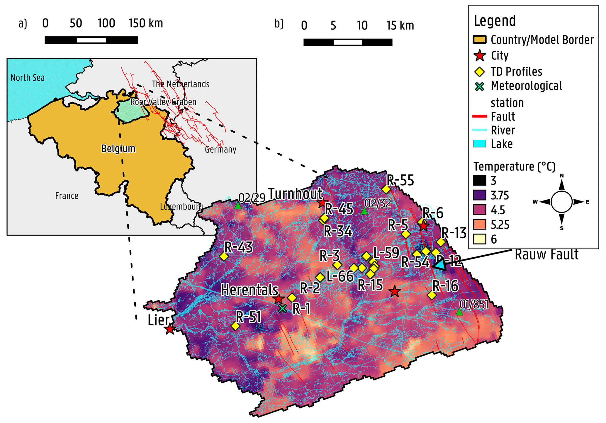
Figure 1Geographical location of (a) the Nete catchment within Belgium with an indication of the faults in the Roer Valley Rift System, as in Vanneste et al. (2013), and (b) the land surface temperature averaged for January 2001 derived from satellite data (MODIS) for of the study area within the Nete catchment.
The Neogene Aquifer is located in the Campine area, in the northeast of Flanders, and is considered to be the most important groundwater reservoir in the region (Coetsiers and Walraevens, 2006). A full description of the study area has been presented elsewhere (Casillas-Trasvina et al., 2021). For clarity, only a brief summary is given here. The area of the Neogene Aquifer within the Nete catchment is studied in this work, as shown in Fig. 1. The area is characterized by a low relief, with altitudes ranging from ∼5 to 70 m (above TAW, Tweede Algemene Waterpassing) along a west–east gradient. As a result, the hydrography is characterized by an east–west drainage system that belongs mainly to the Scheldt river basin (Van Keer et al., 1999; Rogiers et al., 2014). The aquifer is mainly composed of Neogene marine sand deposits that induce some variations in hydrochemical composition, although the groundwater is weakly mineralized (Coetsiers and Walraevens, 2008). The Oligocene (Rupelian) and Mio-Pliocene geology of the study area is presented in Sect. 2. The lithology mainly consists of fine- to medium-grained sands, while the clay content is found to vary in certain units (e.g. Kasterlee, Lillo, and Diest formations), and basal gravels are sometimes present between the units (Laga et al., 2001). The sediments dip towards the north–northeast, with a gentle slope of about 1 %–2 %, with some disturbances towards the west by different normal faults. In the eastern/northeastern part of the study area, faults occur that were formed as a consequence of the development of the Roer Valley Graben (RVG), which is the northwestern-most part of the Lower Rhine Graben (LRG; Verbeeck et al., 2017; Deckers et al., 2018). The most important of these faults outside the proper RVG, and in terms of Cenozoic offset, is the Rauw fault, which is proven to have been active during the Pleistocene (Verbeeck et al., 2017). The Rauw fault has a displacement of more than 7 m in the Quaternary, which increases with depth. It does, however, not have a clear surface expression. The Rauw fault consists of two separate branches (i.e. Rauw fault and Rauw east), around 700 m apart, for which the movement of the Rauw east fault stopped earlier, and Rauw fault has taken over the activity (Verbeeck et al., 2017). For a more detailed description, please refer to Verbeeck et al. (2017).
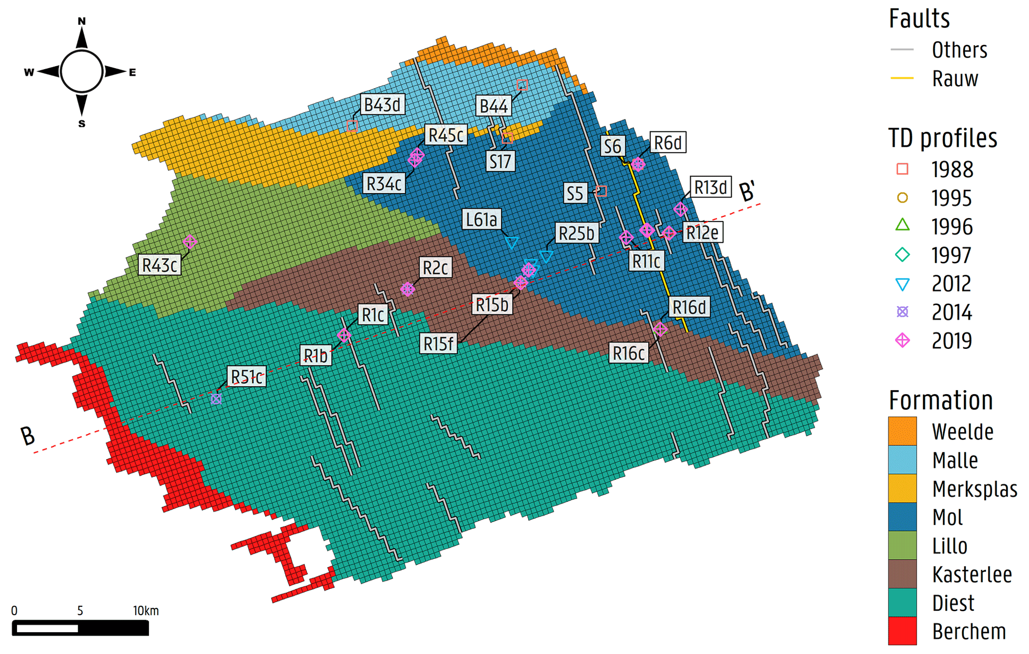
Figure 2Plan view of the study area as discretized in the second layer of the numerical model. It indicates the faults (emphasis on the highlighted Rauw fault), cross section, temperature–depth profile locations, and modelled formations derived from the hydrogeological 3D model in Deckers et al. (2019).
Quaternary deposits of varying texture overlie the Neogene units and constitute the upper few metres of the aquifer system. The hydrostratigraphic units occurring below the Quaternary are composed of Pleistocene and Pliocene sediments. These consists of the Malle, Merksplas, Mol, and Lillo sands, sitting on the Kasterlee Formation, a mixed clayey-sandy formation deposited in shallow marine to estuarine conditions. It is followed by the Diest Sands, overlaying the Lower Miocene Berchem Sands and Late Oligocene Voort Sands. The Boom Clay, an Oligocene marine sediment, forms the lower boundary of the system. For a more detailed description of the hydrostratigraphy of the area and the Boom Clay, please refer to Laga et al. (2001), Coetsiers and Walraevens (2008), Yu et al. (2013), and Vandenberghe et al. (2014). Notwithstanding their lithological differences, Patyn et al. (1989) concluded from hydrogeological observations that these sediments behave as a single aquifer. Similar to Casillas-Trasvina et al. (2021), in this work, the combined Quaternary deposits, Pleistocene, and Upper and Lower Pliocene aquifers, together with the Lower Miocene and Oligocene aquifer system, are referred to as the Neogene Aquifer.
Various subsurface and surface activities are taking place or being planned above and below the Neogene Aquifer, including, but not limited to, surface and geological disposal of low-level and short-lived and long-lived nuclear waste. The Nete catchment and the Neogene Aquifer have been subject to studies in the framework of geological disposal of nuclear waste (Beerten et al., 2010; Gedeon, 2008; Mallants, 2010; Mazurek et al., 2009; ONDRAF/NIRAS, 2010, 2013).
3.1 Data collection
3.1.1 Temperature–depth (TD) profiles
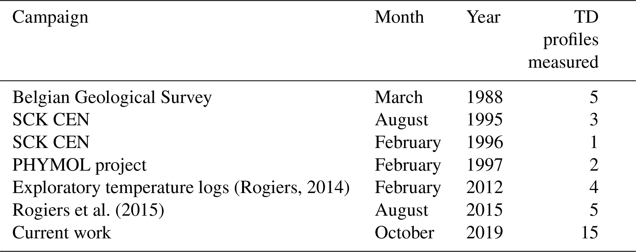
Temperature–depth (TD) profiles have been collected in the framework of various projects and campaigns. Historical data were compiled by Rogiers et al. (2015) from previous campaigns, as presented in Table 1. The quality of the TD profiles taken from 1988 to 1997 is unknown since the sensor resolution and accuracy, together with the performed logging speed (up to four logs per day), are not known, potentially inducing considerable bias in the obtained temperatures. The location of these TD profiles is presented in Fig. 2. The TD profiles collected during the site characterization for the cAt project (ONDRAF/NIRAS, 2010) were not considered during the assessment by Rogiers (2014) since they were believed to be influenced by drilling activities, and thermal equilibrium was not reached yet.
The four TD profiles reported by Rogiers (2014) were the only data for which the type and characteristics of the sensor and logging speed are known up to that date. For these wells, a correction was applied to the raw data to account for the logging error. The properties of the used sensor are presented in Table 2. Another five TD profiles were taken in a second campaign presented by Rogiers et al. (2015). A different temperature logger was used, for which the characteristics are presented in Table 2. The stop–go measurement method by Harris and Chapman (2007) was followed, similar to the previous campaign.
Table 2Summary of temperature sensors used for different campaigns.
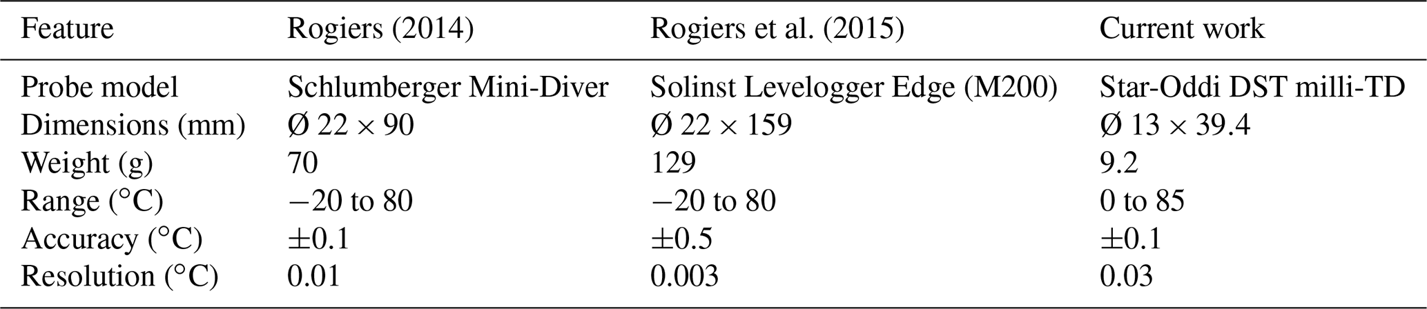
The temperature probe used in this work was the Star-Oddi DST milli-TD (https://www.star-oddi.com/products/data-loggers/depth-sensor-water-level-data-logger-recorder-milli-TD, last access: 7 November 2022). This probe is typically used in TD logging by tagging fish in migration and behaviour studies. It was selected due to its low diameter, making it ideal to overcome a sort of bottleneck observed in a previous campaign. The dimensions of this probe are presented in Table 2, which summarizes the temperature sensors used in this and in previous works. The measuring method described by Bense et al. (2017) and Kurylyk et al. (2018) was followed. In this work, 15 groundwater wells were measured to extend the number of observations spread across the Nete catchment. Finally, a total of 23 different locations were measured with a total of 35 TD profiles (some filters, i.e. R-12 e-f, R-15 b-f, R-16 c-d, R-1 b-c, and R-54 a-c-f, are in the same borehole), ranging from near the surface to roughly −450 m deep and distributed in time and space across the Nete catchment, are used as observations to constrain the heat transport model (see Appendix A1).
3.1.2 Air and soil temperature time series
Several meteorological stations exist within the region, and only three provide measured values of air (at 1.75 m above surface) and soil temperature (measured at 5 cm below surface) within or nearby the study area, i.e. Herentals, Overpelt, and Eindhoven stations. Data from the two stations in the Flemish region, belonging to the Flanders Environment Agency (VMM; https://www.vmm.be/, last access: 7 November 2022), were accessed through https://www.waterinfo.be/ (last access: 7 November 2022). Data from Eindhoven were obtained through the Royal Netherlands Meteorological Institute (KNMI; https://www.knmi.nl/home, last access: 7 November 2022). The temperature–time series for the data gathered for these stations from 1 January 2003 to 31 October 2016 is presented in Appendix A2.
3.1.3 Remote sensing data
Remote sensing data play an important role in the development of validated multi-scale Earth system models (Fick and Hijmans, 2017; Hazaymeh and Hassan, 2015; Tomlinson et al., 2011). Several satellite missions launched by NASA and the ESA (European Space Agency) collect data from the Earth's crust up to the atmosphere on temperature, gravity variations, landscape characteristics, etc. Missions such as Landsat, ASTER, MODIS, and Copernicus collect, for example, land surface temperature (LST) values, which can be freely retrieved from their online platforms. Landsat, Copernicus, Meteosat Second Generation (MSG), and MODIS missions gather global LST values. However, MODIS gathers 1 km resolution images, whereas Copernicus images have a 5 km resolution. For this reason, LST images were retrieved from NASA's MODIS Terra for the region, with 8 d and 8 night averages from 2001 to 2019. These were upscaled to monthly means for our purposes. The resulting raster stack was sampled for the 2001–2019 monthly period in two locations, corresponding to the VMM weather station soil temperatures measured at Herentals and Overpelt. These results are also included in Appendix A2. From this sampling, it is clear that the raster LST images correlate to the soil temperatures from the meteorological station, with the peak temperature values mostly during the summer months. Reinart and Reinhold (2008) discuss this effect on peak values, similarly, by comparing MODIS-retrieved temperature values and in situ measurements. They attribute these higher values to the so-called “skin effect”, since satellite radiometers are only able to retrieve skin temperatures (Reinart and Reinhold, 2008) which are influenced by several other components, i.e. prevailing wind speed, time, and conditions on the day the measurement is taken (Fick and Hijmans, 2017; Tomlinson et al., 2011; Wan et al., 2002). A simple linear regression model was fitted to estimate the LST raster stack in relation to in situ soil temperature measurements from the weather stations (LSTcorr=0.6022 LST + 3.162; R2=0.8; standard errors of slope 0.025 and intercept 0.46; see Appendix A3). Although there seems to be some seasonal hysteresis in the relation between the two, and one could potentially use, for example, the month as an additional regressor, we considered this to be sufficiently accurate for the current work. This temperature estimation was then applied to every LST raster (i.e. every month from 2001 to 2019). An example of the estimated monthly images for year 2001 is shown in Appendix A4. From the estimated monthly images, it is possible to observe the temporal but also the spatial distribution across the catchment.
3.1.4 Holocene paleo-temperature reconstruction
To advance the conceptualization of the transport model and to improve the initial boundary condition for the top of the model (i.e. temperature values), a long-term temperature–time input curve was built using data from several authors. The data were retrieved from the paleo-climatology data library of the National Centers for Environmental Information (NCEI; https://www.ncdc.noaa.gov/data-access/paleoclimatology-data, last access: 7 November 2022). Data from D'Arrigo et al. (2005, 2006), Casty et al. (2007), Buntgen et al. (2011), Tingley and Huybers (2013), Esper et al. (2014), Luterbacher et al. (2016), Langevin et al. (2017), Marsicek et al. (2018), Ljungqvist et al. (2019), and Glaser and Riemann (2009) were used for the estimation of the LST time input curve. The data from these authors present paleo-temperature reconstruction values for the Holocene in Europe in gridded format with coordinates for reference. Data from Mann et al. (2009) and Mann (2002) were used for comparison, since they represent a general and internationally accepted Northern Hemisphere temperature–time curve. The values from these authors were either taken from the gridded value or from values that contained Flanders within its/their boundaries. The obtained values from each author curve were then scaled to the relative Belgian average temperature for the period 1961–1990, as derived from Jones et al. (1999, 2012). These temperature–time curves are shown in Appendix A5. Inverse distance weighting (IDW; ) was performed on the data locations with reference to the centre of the groundwater model domain. The resulting weights were used to determine an IDW average time series, for which the yearly (IDW – 1 year) average is displayed in Fig. 3. Recursive partitioning segmentation (RPS) was done using an implementation of the Lavielle (1999, 2005) method. This method was applied to different sections of the IDW-averaged temperature–time curve, aiming to obtain a segmentation from −8500 to 2000 (CE, common era) using average step sizes of 1 kyr (−8500 to −500), 100 years (−501 to 1500), 10 years (1501 to 1950), and 1 year (1951 to 2000). Monthly values for the last 19 years from remote sensing land surface temperature data were included at the end of the segmentation (see Fig. 3). A total of 90 time steps are then included to the steady-state solution to determinate the initial temperature, thus aiming to improve its efficiency.
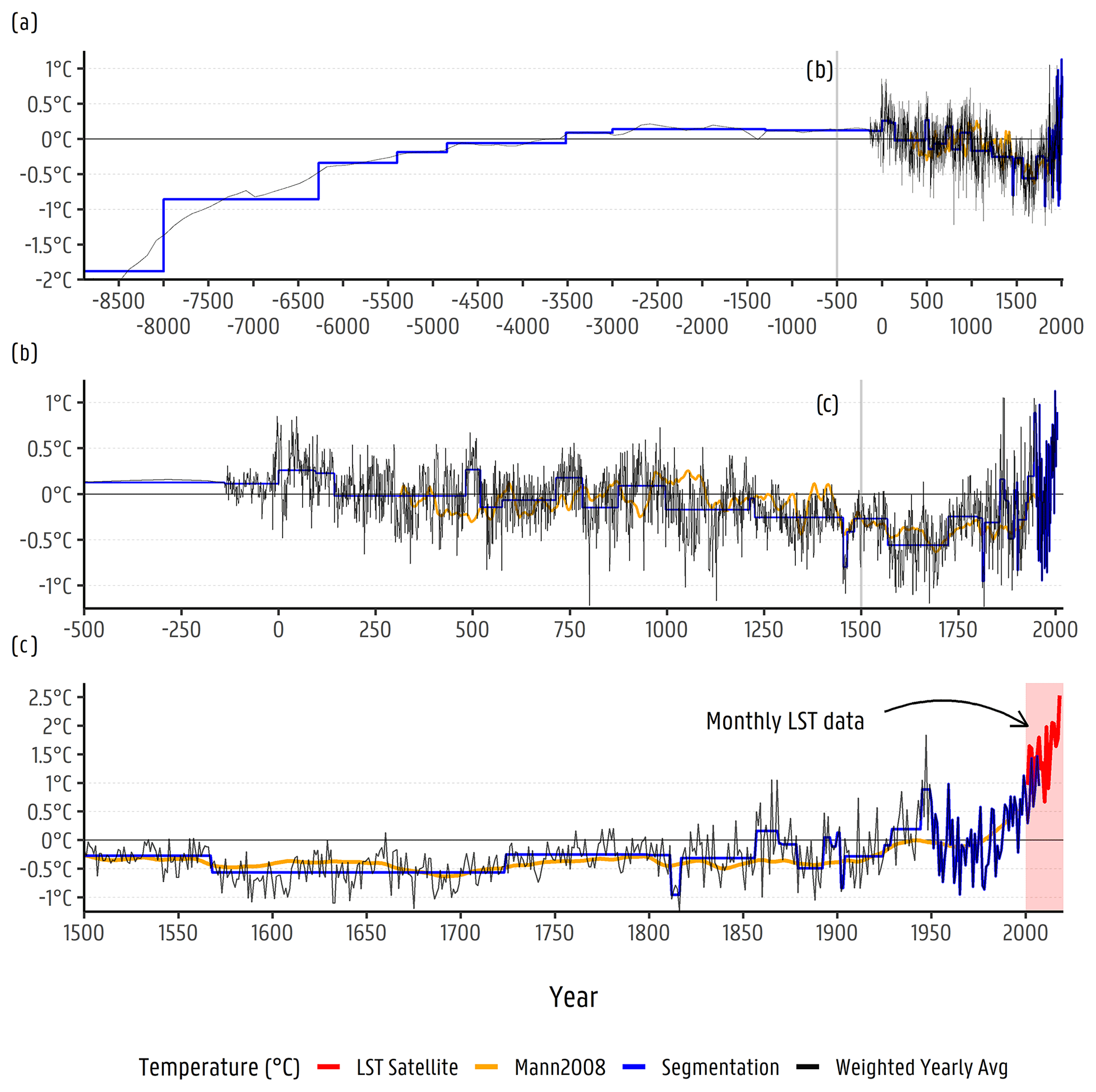
Figure 3Temperature–time curve to use as input in a transient heat transport simulation indicating the time step sizes for the last 10 519 years.
3.2 Modelling framework
For the current work, the Neogene Aquifer model (NAM), a steady-state groundwater flow model constructed by Casillas-Trasvina et al. (2021) using MODFLOW-2005 (Harbaugh, 2005), is used. A heat transport model by Rogiers et al. (2015) has been updated using MT3D-USGS (Bedekar et al., 2016) and is used for simulations. The models were developed and post-processed using the RMODFLOW (Rogiers, 2015, 2016a) and RMT3DMS (Rogiers, 2015, 2016b) packages for R (R Core Team, 2020).
3.2.1 Conceptual model
The NAM by Casillas-Trasvina et al. (2021) has a lateral boundary that coincides with the catchment boundaries of the Kleine and Grote Nete rivers. Similar to Gedeon (2008), the catchment is assumed to be laterally isolated, so no groundwater flow across the lateral boundary occurs. The top boundary is put at the ground surface elevation, while the bottom boundary coincides with the top of the Boom Clay formation (from a few metres below the surface up to roughly 450 m deep). The Neogene Aquifer becomes deeper in the northeasterly direction from the southwestern corner where the Boom Clay is present at the ground surface. The groundwater flow in the Neogene Aquifer is driven mainly by surface hydrological features (i.e. recharge and rivers) creating several local flow systems with local influences of abstraction wells. It is assumed to be in dynamic equilibrium, with no long-term trends in groundwater flow, which allows for a steady-state simulation (Gedeon, 2008). Casillas-Trasvina et al. (2021) included the conceptual model consideration that fault planes have hydraulic properties distinct from the surrounding sediments and do not penetrate up to the surface as they are buried by at least a thin Quaternary cover. Additionally, these planes are assumed to act as barriers if they behave in a significantly different way to the surrounding sediments, thereby affecting the horizontal component of the groundwater flow. Together with their buried nature, this causes upward flow at the upgradient side of the fault. On the downgradient side of the fault, the vertical flow direction may also be affected, turning into a more parallel direction in respect to the fault. Finally, groundwater may be overflowing above the fault plane if it acts as a strong flow barrier, given the fact that the fault is buried, creating a groundwater level step (head difference).
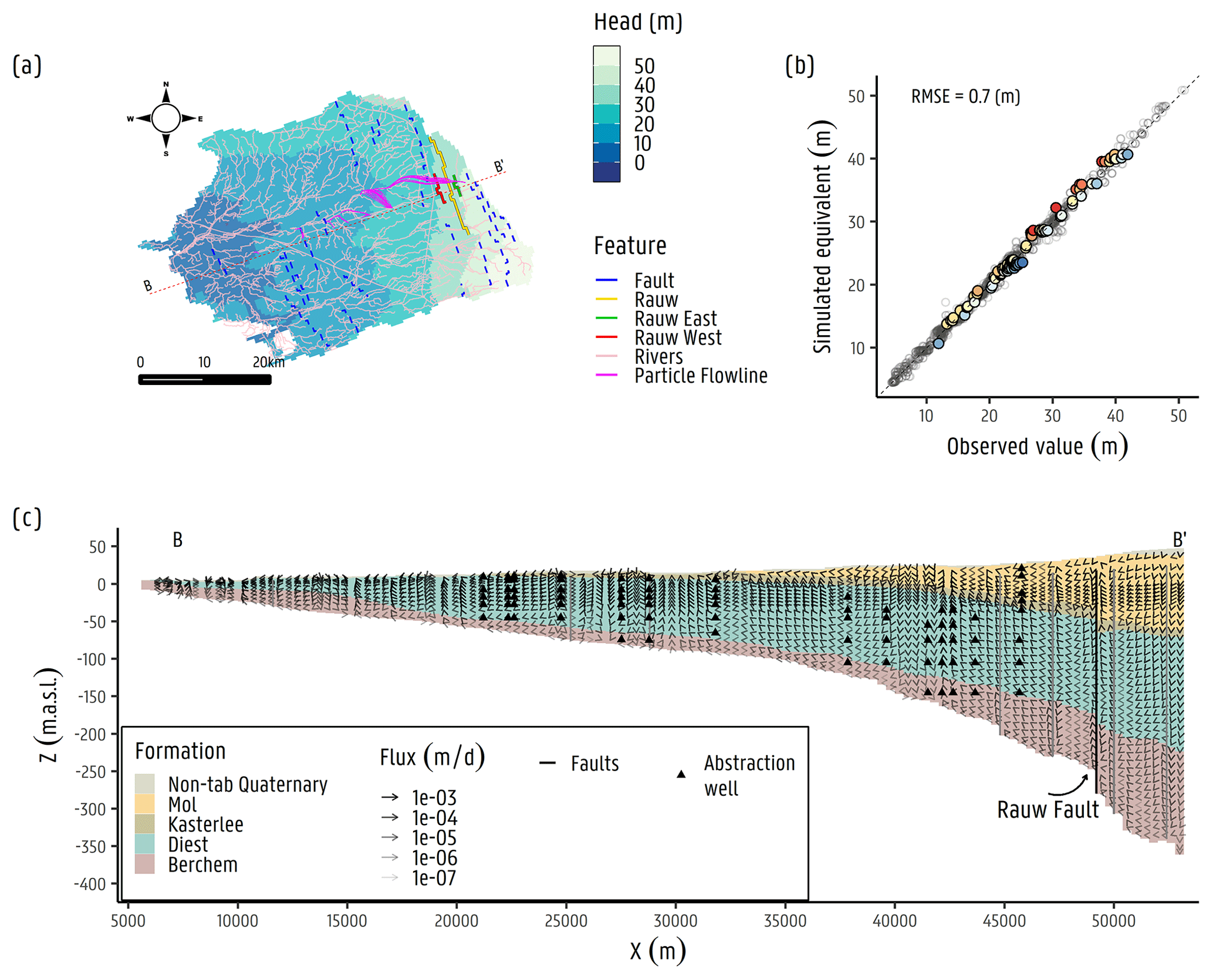
Figure 4Groundwater flow model results adapted from Casillas-Trasvina et al. (2021). (a) The hydraulic head distribution over the Nete catchment. (b) Scatterplot of simulated equivalents and observed hydraulic heads. (c) Cross section B–B' with arrows indicating the flow magnitude (m d−1) and direction.
3.2.2 Groundwater flow model
The structural updates into NAM for heat transport follow the latest hydrostratigraphic 3D model for Flanders (H3D) by Deckers et al. (2019). Similar to NAM by Casillas-Trasvina et al. (2021), it assumes nine hydrostratigraphic units, i.e. non-tabular Quaternary (Quaternary cover above the Kempen aquifer system), Weelde, Malle, Merksplas, Mol, Lillo, Kasterlee, Diest, and Berchem and Voort, of which the geometry is based on Deckers et al. (2019). The model domain is discretized into 49 vertical layers that thin out closer to the surface to ensure smaller modelling cells close to surface hydrological features where groundwater gradients are the highest. The bottom of layers 1 and 2 were assigned equal to 50 % and 30 % of the ground surface elevation. The bottom of layer 3 was set equal to 0 m a.s.l. (above sea level; TAW). From layer 4 to layer 9, layer thicknesses of 5 m are used. From layer 10 to 49, the thickness used is 10 m. The modelled area was discretized into a regular model grid of 96 rows and 146 columns, resulting in cells with dimensions of 400 m × 400 m. A total of 23 faults were simulated with the horizontal flow barrier (HFB) package (Harbaugh et al., 2005), starting from the top of the second numerical layer (from around 12 to 18 m below surface) to the bottom of the modelled domain, given that the faults do not present a clear surface expression (Verbeeck et al., 2017). Rivers, lakes, canals, and abstraction wells are defined in the groundwater flow model. The groundwater abstractions range from a few cubic metres per day (m3 d−1) to more than 300 m3 d−1. Data from several sources were used to define these parameters, including the Flemish hydrographic atlas (Vlaamse Hydrografische Atlas, VMM 2017) and the IGN/NGI dataset (IGN/NGI 2017). Spatially distributed recharge is implemented with values obtained from DiCiacca (2020), which are derived from vegetation cover, soil texture, and spatial input layers of depth to the groundwater table, based on hydraulic head observations. A scaling factor was used during the model inversion for the calibration of the recharge initial value. A total of 1393 averages from hydraulic head time series are used in the NAM. These observations were obtained from the piezometric network monitored and maintained by SCK CEN for ONDRAF/NIRAS and from the subsurface database for Flanders (Databank Ondergrond Vlaanderen, DOV). The model performance of the NAM model had a root mean square error (RMSE) of 0.70 m, accounting for a total head loss of 46.5 m. Figure 4a–c show results from the groundwater flow model, including (a) the hydraulic head distribution over the Nete catchment, (b) the scatterplot of simulated equivalent vs. observed hydraulic head observations, and (c) a cross section (B–B') with arrows indicating the flow magnitude results from the groundwater flow model per model cell. Appendix A6 shows a cross section with derived Péclet numbers (Pe), following Freeze and Cherry (1979; ), relating the rate of flow advection to the diffusion. In here, a value of m2 s−1 for the diffusion coefficient (De) is used, corresponding to the tritium diffusion coefficient in pure water (Gedeon, 2015), and a value of L=200 m, corresponding to a rough average distance from the bottom of the aquifer to the surface, is used. It is notable that Pe≫1 is in the formations above Berchem and Voort sands, thus being more advection–dispersion-dominated areas. On the other hand, in the deepest areas of the aquifer (i.e. Berchem and Voort sands), Pe≤1, and therefore diffusion becomes an important transport mechanism. The values of Pe≤1 are very few, mostly near to 1, and found near the bottom of the aquifer where groundwater flow velocities are at the lowest. In these areas, the fluxes occur near the bottom no-flow boundary of the model. Research has been previously performed, as summarized by Vandersteen et al. (2013), which pointed out the low hydraulic conductivity values for the Berchem and Voort formations (as low as 0.02 m d−1), which are thus not particularly acting as a barrier/clay but have modest advective/diffusive behaviour. A more detailed description of the NAM structure, parameters, and results is presented in Casillas-Trasvina et al. (2021).
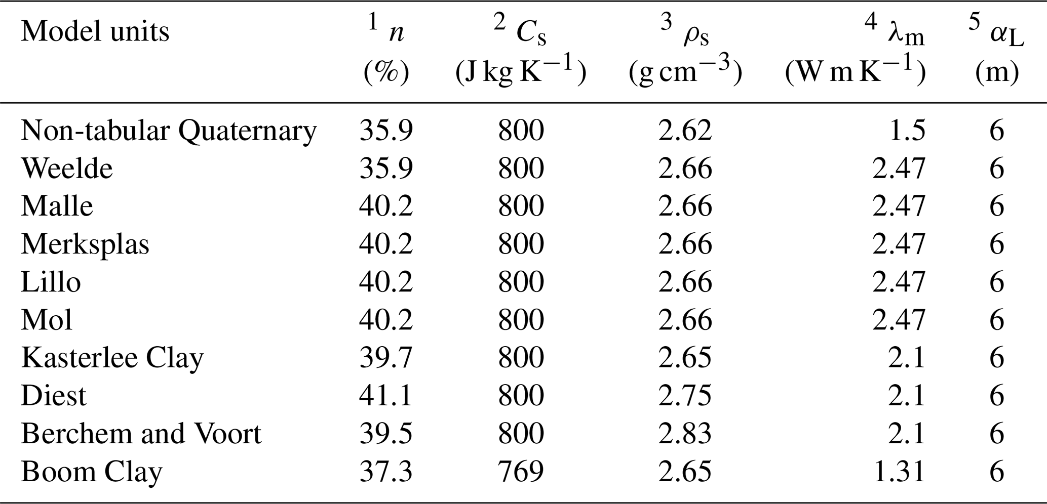
Table 3Overview of the hydrogeological unit properties used for the updated version of the NAM heat transport model in MT3D-USGS parameter names, where 1 n is the porosity, 2 Cs is the specific heat capacity, 3 ρs is the density of the solid phase, 4 λm is the thermal conductivity, and 5 αL is the dispersivity.
3.2.3 Heat transport model development
Numerical modelling
In Liu et al. (2019) and Hecht-Méndez et al. (2010), it is demonstrated that MT3DMS is able to simulate heat transport, when temperature variations are limited, through the analogy with solute transport. If large variations in temperature are to be modelled (i.e. an aquifer thermal energy storage (ATES) and a ground source heat pump (GSHP) with large ranges), then a model that accounts for variable density and viscosity terms (e.g. SEAWAT, Langevin et al., 2008; SUTRA, Voss and Provost, 2010; FEFLOW, Trefry and Muffels, 2007) should be applied. But, in the current setting, we do not consider this to be relevant. The heat and solute transport equations formulated in analogous forms show how MT3DMS can be used for heat transport simulations. For single species, the solute transport equation solved by MT3DMS (Langevin et al., 2008) as follows (Eq. 1):
where φb is the bulk density (mass of the solids divided by the total volume; M L−3), Kd is the distribution coefficient of the solute (L3 M−1), θ is the porosity (–), C is the concentration of the solute (M L−3), ∇ is the Vector differential operator, Dm is the molecular diffusion coefficient (L2 T−1), α is the dispersivity tensor (L), q is the specific discharge vector (L T−1), Cs is the source concentration of the solute (M L−3), and is the source or sink of the fluid (T−1).
The analogous equation (Eq. 2) for the heat transport is defined as follows:
where T is the temperature (∘C), ps is the density of the solid (M L−3), φCp fluid is the specific heat capacity of the fluid (L2 T−2 ∘C−1), φCp solid is the specific heat capacity of the solid (L2 T−2 ∘C−1), KT bulk is the bulk thermal conductivity of the aquifer (M L3 T−2 ∘C−1), and Ts is the source temperature (∘C).
When the more recent MT3D-USGS code (Bedekar et al., 2016) is used to simulate heat transport, then these equivalent transport parameters are defined. The heat dispersion is the same as solute dispersion, which is determined by longitudinal and transversal dispersivities. For a more detailed description, the reader is referred to Anderson (2005), Langevin et al. (2008), Zheng (2010), Bedekar et al. (2016), des Tombe et al. (2018), and Liu et al. (2019).
Modelling set-up
A heat transport model of the original NAM (Gedeon, 2008) using MT3DMS (Zheng, 2010) has been constructed by Rogiers (2015). In this model, the top boundary condition uses a yearly average value for the temperature imposed on the ground surface. The transport simulation covered a period of 10 519 years with yearly time steps, covering almost the entire Holocene period. The set temperature as a boundary condition at the surface accounted for the topographical influence and land cover classes, based on data presented by Leterme and Mallants (2012). A heat flow density of 0.06 W m−2 was set to the bottom boundary condition, with the value being in accordance with the average heat flow density reported by Pollack et al. (1993) for Cenozoic and Mesozoic sedimentary and metamorphic crust (Rogiers et al., 2015). The specific heat capacity, φCp fluid, and density, pw, of the fluid (groundwater) were set to 4193 J kg−1 K−1 and 999.7 kg m−3, respectively (Rogiers et al., 2015). Material properties defined in the model were (a) total porosity (θ), (b) specific heat capacity (φCp fluid), (c) density of the solid (ps), (d) thermal conductivity (λm), and dispersivity (α).
In this work, similar to Rogiers et al. (2015), we based the material properties on the reported literature values found in Hoes et al. (2005), Beerten et al. (2010), Chen et al. (2011), Govaerts et al. (2011), and the WTCB methodology reported in van Lysebetten et al. (2013). These values and a summary of the hydrologic properties required to parametrize the MT3D-USGS model used in the simulations are shown in Table 3. Note that the potential impact of geothermal heat flow of an increasing temperature with depth on viscosity and density of the fluid is not considered. This assumption is reasonable, as we consider a not so deep groundwater flow system (<500 m) in which these temperature effects will be of minor importance (Bense and Person, 2006; Person et al., 1996) and where emphasis is not put on surface water/groundwater interactions when the impact on viscosity derived from temperature gradients may be considerable (Engelhardt et al., 2013; Kurtz et al., 2014; Liu et al., 2019; des Tombe et al., 2018).
Building on the previous work, the latest version of the heat transport model built by Rogiers et al. (2015) has been updated from MT3DMS (Zheng, 2010) to MT3D-USGS (Bedekar et al., 2016), following the new hydrostratigraphy and grid discretization used for the updated NAM groundwater flow model by Casillas-Trasvina et al. (2021). The dispersivity was based on a scale of 200 m, which is a rough measure for the depth of the aquifer, and thus the travel distance of heat. The linear dispersivity–scale relationship was derived from the literature data, as presented by Rogiers et al. (2013). For simplicity, the dispersivity is considered to be constant, with longitudinal dispersivity αL equal to 6 m, and the ratios of transverse and vertical transverse dispersivity to αL equal to 0.1 and 0.01, respectively.
Top boundary condition
As the first modelling step, a steady-state finite difference solution was obtained using temperature from −8500 ka as the top boundary condition. This was used as the initial temperatures for transient simulations. The transient model is run for 10 519 years, from −8500 ka to 2019. Every single time step is derived, as explained above in Sect. 3.1. A yearly average value from the LST raster stack was determined to be used as the spatial distribution for the Holocene paleo-temperature distribution implemented in the model as a top boundary condition. The temperature spatial distribution was derived from satellite data and used directly in the monthly part of the transient simulation. The 1 km LST rasters were downscaled to 100×100 using the {raster} package function disaggregate in R. Then, the mean values within a modelling cell was estimated for every 1 km LST raster that were sampled in the centre of each active model cell (MODFLOW model) with a 400 m × 400 m resolution. A total of 316 rasters were produced from −8500 ka to 2000, and one for each month, from January 2001 to October 2019. Each of these rasters represent a time step for the transient transport simulation.
Paleo-temperature boundary condition test
To increase the accuracy of the simulated temperature and hence have a good simulated vs. observed temperature performance, the simulated temperature has to be able to stabilize (or reach a steady state). Thus, we require the estimation of initial conditions (initial temperature values for each stress period).
To show the importance of performing the paleo-temperature simulations to provide initial conditions for further stress periods, a test was performed. The (disturbed) simulations increasing by 1 ∘C in temperature at the initial top boundary condition at various time steps (i.e. 10 000, 9000, 8000, 7000, 6000, 5000, 4000, 3000, 2000, 1000, 900, 800, 700, 600, 500, 400, 300, 200, and 100 ka) and for the remaining of the simulation period were performed. The simulated temperature–depth (TD) profile from all these models was obtained for the same location (on well R-54f). The results of this test are shown in Fig. 5. In Fig. 5a, the simulated TD profile at the last time step (present time) from a normal (undisturbed) forward model run is shown. In Fig. 5b, the figure shows the differences between the disturbed and normal (undisturbed) simulated TD profiles, pointing out the time required for the model to reach a steady state, given a change of 1∘ in the top boundary temperature condition. This supports the use of a relatively long time series, which is actually a process that is not computationally intensive. The model has 337 stress periods in total and runs for around 40 min. For the nine time steps in the stress period between 10 000 and 2000 ka (in steps of 1000 years) it requires around 1 min (approximately 64 s) to compute a temperature stabilization of up to 30 % per temperature degree of change in the temperature top boundary condition. Having a higher-frequency temperature distribution is not within the scope of this work, as we are more interested in knowing what improvement the implementation of an additional state variable may bring to the conceptualization of the groundwater system rather than aiming for higher-frequency results for which monthly time steps seem reasonable.

Figure 5(a) Temperature–depth (TD) profile simulated at observation well (i.e. R-54f) at the end of the coupled groundwater flow and heat transport undisturbed simulation (present time). (b) Temperature difference at the same observation well between the TD profile at the end of each disturbed simulation (present time) minus the undisturbed simulation.
Similar to what has been done in previous work in this research area (Casillas-Trasvina et al., 2021; Gedeon, 2008; Rogiers et al., 2015), and as indicated in Sect. 3.2.1, the aquifer is assumed to be in dynamic equilibrium with no long-term trends in groundwater fluxes, which allows us to simulate the groundwater flow in a steady state. For the purposes of our research, we find this assumption acceptable.
Model calibration
Automatic parameter optimization was implemented as a technique for model inversion. Several algorithms were used for global model optimization such as the Standard Particle Swarm Optimization (SPSO11; Clerc et al., 2012; Zambrano-Bigiarini et al., 2013; Zambrano-Bigiarini and Rojas, 2013) and differential evolution (Mullen et al., 2011). Temperature gradients, calculated by fitting a cubic smoothing spline with a knot distance of 1 m derived from each TD profile, and hydraulic head values were used as calibration targets during the joint inversion procedure. Results from the spso11 algorithm were selected for minimizing the RMSE despite requiring a slightly longer computational time.
3.2.4 Modelling strategy
Model 1: baseline
The updated version of the groundwater flow model by Casillas-Trasvina et al. (2021) and the heat transport model, including the Holocene temperature–time curve and satellite data for the last 19 years, is defined here as the baseline model (Paleo RPS). The heat transport simulation is jointly inverted with the groundwater flow model against temperature gradients and hydraulic head observations, respectively. The results from this model are compared against model case 2 and model case 3 (see below) to estimate the effect of thermal conduction and normal faults in the temperature distribution in the Neogene Aquifer across the Nete catchment. Additionally, a model without the effect of the paleo-temperature and including only the LST temperatures of the last 19 years (named the monthly LST model) and a steady-state transport model are also evaluated in comparison to the defined baseline model.
Model 2: thermal conduction
A model case accounting for only the thermal conduction is performed to enable the quantification of the effect of groundwater flow on the subsurface temperature distribution. The baseline simulation accounts for both the advection of heat via the groundwater flow and thermal conduction. For this second simulated model without groundwater flow, the same parameter set is used, but the advection of heat is switched off. The difference between the first and second simulation temperature distributions then gives us the changes in temperature induced by the groundwater flow.
Model 3: heat transport without faults
An exploration of the temperature distribution in the aquifer without faults (i.e. no HFB included in the flow model by Casillas-Trasvina et al., 2021) is also performed. For the heat transport model, parameters are set to be the same as for the baseline model. Both this case and the baseline model account for both the advection of heat via groundwater flow and thermal conduction. The difference between both of these cases allows the quantification of the effect of faults on the temperature distribution and provides an idea of the parameter sensitivity of the hydraulic conductivity of such structures.
4.1 Paleoclimate effect on temperature distribution
Every measured TD profile is compared with its respective simulated temperature based on its spatial and temporal (i.e. month and year) location. A scatterplot of the model-simulated temperature gradient values vs. the observed measurement is shown in Fig. 6a, where a comparison is made between the monthly LST model (see Sect. 3.2.4; model 1 – baseline) and the baseline model of the current work (Paleo RPS), separating the observations with a z value below and above −5 m a.s.l. Note that temperature/geothermal gradients are more important than absolute temperature values as they provide more insights to groundwater fluxes. The gradient is calculated by fitting a cubic smoothing spline with a knot distance of 1 m. A steady-state transport solution result is also included for reference. From this scatterplot, both transient heat transport simulations have a bias towards lower gradient values, indicative of flux magnitudes being potentially overestimated. Additionally, most of the simulated values above the m a.s.l. limit show large fluctuations. This may be explained by the imposed temperature value as the top boundary condition (at the first layer of the model), the potentially heterogeneous properties of the materials near the surface, and the space–time discretization of the model (i.e. dimensions of the cells and time step sizes). The spatial variations in the imposed temperature (i.e. scaling of the thermal images/model cell size vs. the scale where TD profiles were measured), together with the local flows occurring near the surface of the model affected in very local scales (e.g. surface/groundwater exchanges), participate in these fluctuations that seem to stabilize at around −5 m a.s.l. depth. At these shallow depths, temperature variations can drive fluctuations in heat transport related to the fluid viscosity (Hecht-Méndez et al., 2010; Liu et al., 2019; des Tombe et al., 2018), which are limited to these few metres (∼20 m) below the surface. Additionally, although yearly and monthly time steps were defined in the model, seasonal/diurnal temperature changes may also affect the propagation of heat into the subsurface (Benz et al., 2018; Dong et al., 2018). Nevertheless, the simulated results present an acceptable compromise between observed and simulated values. The paleo-temperature reconstruction model results are more clustered and less disperse, despite having some values spreading at a lower simulated equivalent gradient, in comparison with the LST transient model (see Fig. 6c), thus indicating that this simulation is, overall, slightly more accurately representing the observed situation (RMSE = 0.03 ∘C m−1; 1.15 ∘C), though several inaccuracies are observed in deeper parts of the aquifer (Fig. 6c).
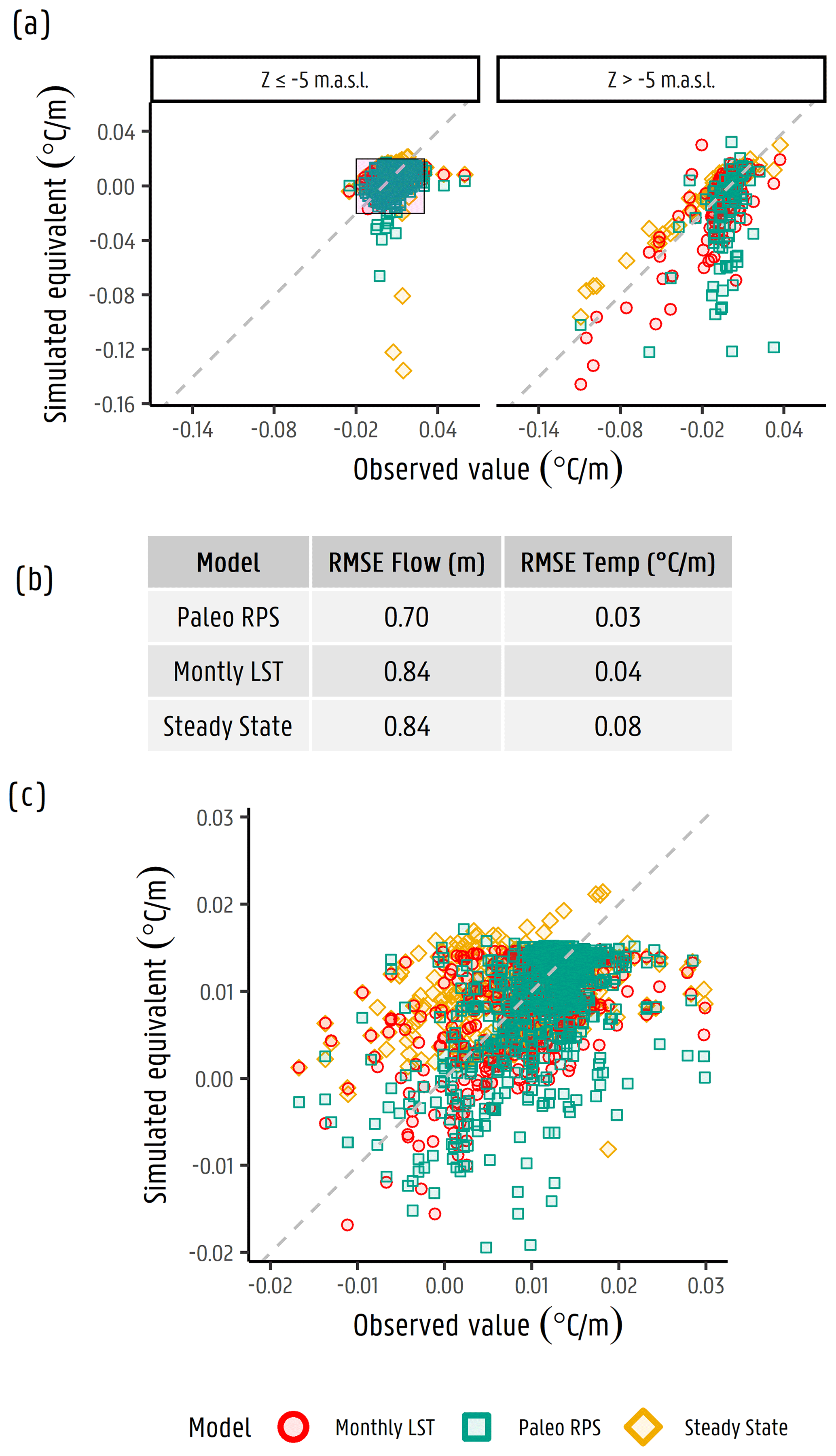
Figure 6Simulated vs. observed temperature gradients showing results from the steady-state model and the monthly LST model and reconstructed paleo-temperatures included as input into the transient model. (a) A distinction is made between observations below and above m a.s.l. (b) The RMSE performance of different models in terms of the hydraulic head (flow model, m) and temperature gradient (∘C m−1). (c) A magnification of the simulated and observed temperature gradients shown in panel (a).
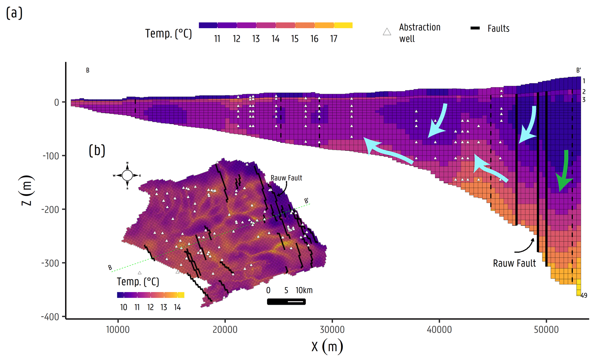
Figure 7Temperature distribution at the last transport step for the paleo-temperature transport model in the (a) cross section. Green and cyan arrows indicate flow systems and fluxes on the east and west side of the Rauw fault (b) and the plan view from model layer 10, indicating a cross section (B–B') for panel (a).
4.2 Current temperature distribution
The flow and transport parameter composite scaled sensitivities (CSSs) with respect to hydraulic head and temperature gradients, respectively, are shown in Appendix A7, with the parameter names shown in Table A1. It can be seen that the flow parameters have a much larger effect on the model results than the temperature parameters, implying their relevance to the produced results. In terms of temperature, the Diest Formation thermal conductivity presents the highest sensitivity, given that most of the temperature profiles were taken at these depths. On the contrary, the Berchem Formation (Berchem and Voort sands), which does not have a large number of observations, presents a relatively high sensitivity as well. Given that, at these depths, the magnitude of groundwater flow is very low (around – m d−1), the transport of heat is less advective and more driven by thermal conduction. Nevertheless, in general, flow model parameter sensitivities are far larger than those for the heat transport model, given that thermal properties have less variation than the hydraulic ones (Saar, 2011).
The temperature distribution at the end of the calibrated heat transport model simulation is shown in Fig. 7. In Fig. 7a, a cross section B-B' is shown, as indicated in Fig. 7b. Figure 7a shows a distribution that closely relates to groundwater flow, as seen in Fig. 4c, indicating the influence of advection. At the east of the Rauw fault, colder water infiltrates, travels downwards, and mixes with warmer groundwater from the bottom of the aquifer. Groundwater with a slightly higher temperature is transported upwards before penetrating the Rauw fault; however, most groundwater flows across the fault at around −150 m a.s.l. Then, upstream of the Rauw fault, a portion of the groundwater flowing upwards overflows above it to then continue its flow direction downwards, mixing again with colder infiltrated water at the western end of the Rauw fault. Groundwater to the west of the Rauw fault then is mixed with colder and younger infiltrated water, reducing its temperature along the approximate flow direction (i.e. to the west) until the end of the fault block, and then continues flowing laterally to the west, merging with another more local flow system. This can be seen in Fig. 7b, which displays the model layer 10, where groundwater temperature to the west of the Rauw fault zone is higher than to the east. Groundwater in this zone is largely influenced by the surface water features carrying groundwater from deeper in the aquifer that has already crossed the Rauw fault. Groundwater to the west of the Rauw fault seems to have a lower temperature, given that mixing with warmer groundwater occurs deeper, near the bottom of the aquifer.
In the shallower parts of the aquifer ( m a.s.l.; Fig. 7a), some “isolated zones” with lower temperatures can be identified in the vicinity of other faults (i.e. from east to west; represented as black dashed lines). These isolated zones correspond to the groundwater flow distribution producing local flow systems in the area formed by the relatively large density of rivers and canals. Even though the faults in the vicinity have a relatively low sensitivity (see Appendix Fig. A7), these might still have an effect on the distribution of temperature. In their review, Irvine et al. (2012) mention that, although thermal properties might have low variations, as stated by Saar (2011), these variations might have a reasonable effect on the overall temperature distribution in sedimentary environments (Chang and Yeh, 2012; Constantz et al., 2003; Hidalgo et al., 2009), such as the Neogene Aquifer. On the other hand, in the deeper parts of the aquifer (near the bottom of the aquifer; Fig. 7a), higher temperatures are present (close to the main source of heat to the aquifer). At these depths, groundwater fluxes are low ( m d−1), which would indicate that the heat transport here would be mostly conduction driven. The discharge zone of the aquifer downstream to the Rauw fault location seems to have some influence from the surface water network driving deep groundwater to the surface. Groundwater abstractions in this zone seem to have an impact, added to the effect of the surface water network, driving heat from deeper parts of the aquifer into more superficial groundwater flow systems.
At the eastern side of the Rauw fault, colder temperatures are found from infiltrating water up to m a.s.l. At approximately this elevation, infiltrating colder water mixes with warmer groundwater from the bottom of the aquifer (Fig. 7a; green arrow), delineating an area where the mixing of younger and older groundwater seems to occur that appears to be defined by the flow velocities characteristic of the hydrostratigraphic formations ( m a.s.l., at around the limit of the Diest Formation with Berchem and Voort formations). On the other hand, at the western side of the Rauw fault zone, an intercalation of the local flow systems is seen, following the east-to-west flow direction (Fig. 7a, cyan arrows, from east to west), as (i) the infiltration area with colder waters, (ii) an upwards groundwater flow driven by the surface water network and groundwater abstractions, (iii) the infiltration area with cold water, and (iv) an upwards groundwater flow. In the section where the aquifer becomes thinner at around 100 m thick (around the centre of the aquifer) towards the west, several even narrower local flow systems occur (as seen in Figs. 4c and 7a). Although these patterns are difficult to discern in the current figure, the majority of the temperature anomalies indicate upward fluxes, which can be explained by the relatively larger density of rivers and drains in the area.
Selected locations along the approximate flow direction where TD profiles were measured are shown in Fig. 8a. Their measured and calculated TD profiles for the three modelled cases (i.e. Paleo RPS, only conduction, and without faults) are shown in Fig. 8b (all measured TD profiles are shown in the Appendix). From east to west, the measured sites are R-13d (to the east of the Rauw fault), R-54c, R-11c, R-15f, R-2c, R-34c, R-1b, R-51c, and R-43c (to the west of the Rauw fault). All measurements show a C-shaped profile, which is an indication of transient conditions at the surface (Anderson, 2005; Bense et al., 2017). From Fig. 8b, the simulated and observed temperature values show that the closer the TD profiles were taken to the fault (R-54c being the closest one), the larger the absolute temperature error is for either of the three simulated cases. The simulated temperature at R-54c is lower than observed, which can be explained by its close proximity to the Rauw fault (of around 10 m apart) and thus being largely influenced by the flux across it, which might be overestimated, as indicated by the lower RMSE by the simulation case accounting only for the thermal conduction. The results from the simulation only accounting for the thermal conduction show the overestimation of the groundwater fluxes in few locations, which are mostly those located from the centre to the east of the studied area. Although the disparity in the model performance is relatively small, it shows the influence that the dense network of rivers and lakes in this zone has on the temperature distribution. Towards the west, where the density of rivers is lower and the aquifer becomes thinner, these differences become nearly negligible. The complete temperature–depth profile time series simulated by the paleo-transport model is included (grey lines), indicating the range of potential temperature values that this model with these specific boundary conditions and heat source can achieve. These paleo-temperature simulated values, starting low, seem to stabilize after several transport steps, achieving an apparent relatively steady condition in the deeper parts of the aquifer ( m a.s.l.). Similarly, as presented by Dong et al. (2018) and Benz et al. (2018), long-term temperature variations in the top boundary condition are potentially driven by external factors such as climate change or changes in land use/cover. These factors seem to have an influence on temperature observations at depths of around −50 m a.s.l. or shallower, according to Fig. 8b. In Fig. 8a, the complexity of the river and canal network is visualized, and several lakes close to the measured sites can be observed. These lakes might explain anomalies occurring relatively close to the surface, but given that groundwater is mainly driven by the surface water network, they represent a likely driver for these shallow variations, potentially driving deeper/warmer waters upwards. Given that the simulated and measured temperature gradients are in fair agreement, the surface water network might have some influence on the temperature top boundary condition for which LST temperature images and the paleo-temperature time curve might not be accounting.
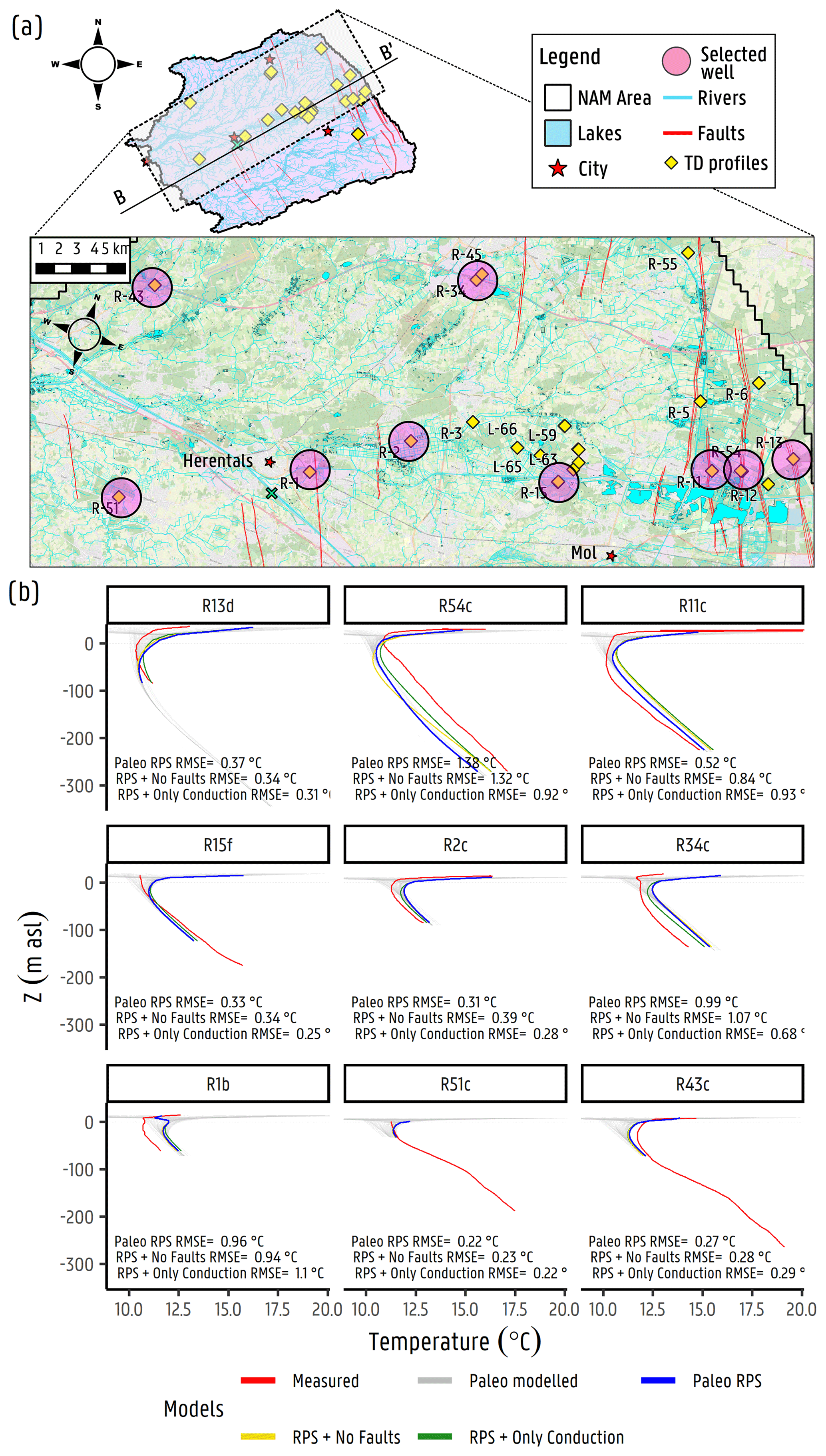
Figure 8(a) Map showing selected TD profile borehole locations (magenta circles) along the approximate flow direction for R-13d, R-54c, R-11c, R15f, R-2c, R34c, R-1b, R51c, and R-43c. The background map source: © OpenStreetMap contributors, 2020. Distributed under the Open Data Commons Open Database License (ODbL) v1.0. (b) Temperature–depth profiles of selected boreholes and their filters (in lowercase letters) showing simulated values for the paleo-temperature model (baseline) and for simulation cases 2 and 3 (only thermal conduction and without faults, respectively). Modelled TD profiles for every time step of the baseline case are also included (in grey, paleo modelled).
4.3 Temperature distribution cases
A comparison between the simulated temperature fields by the baseline (paleo-temperature reconstruction) model versus (a) thermal conduction only (no advection) and (b) without faults as HFB is shown in Fig. 9 and described here.
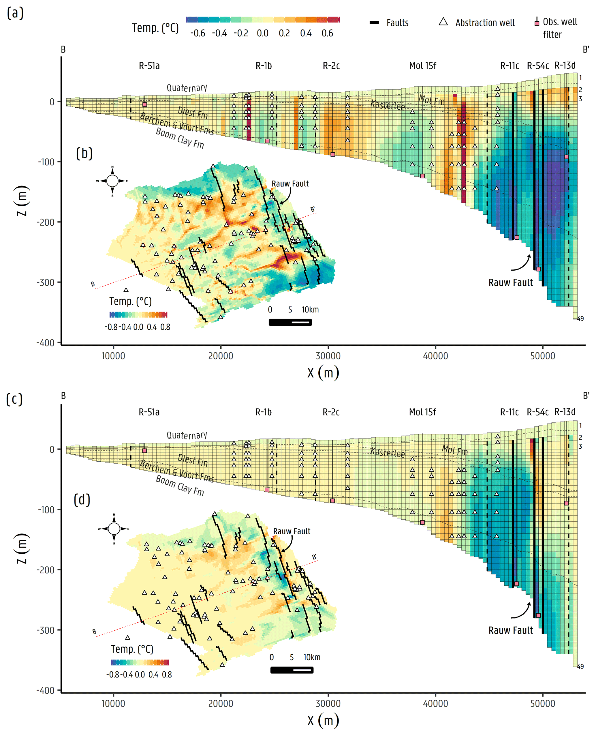
Figure 9Cross sections and plan view (model layer 10) showing the differences between the baseline model minus both cases, with panels (a, b) for the thermal conduction only case and panels (c, d) for the temperature distribution without faults.
4.3.1 Thermal conduction case
Local flow systems patterns
Removing the advection transport mechanism would allow temperature to be freely conducted without being transported by the groundwater flow. It is clear that advective groundwater flow has a large impact on the simulated temperature fields, and thus it is one of the main mechanisms for heat transport in the Neogene Aquifer (see Fig. 4). Given that advection is not being considered (no temperature convection), Fig. 9b clearly shows a temperature pattern that mimics the surface water network. This strongly supports the statement that heat transport in the aquifer may indeed be mainly driven by the advection in local flow systems, where temperatures increase near rivers and streams at the surface by deep groundwater discharge, and by large advection related to groundwater abstractions. The intention of this case is not to determine which case is more or less accurate than the other, as it is known that advective transport exists and not including it would not be realistic, but to highlight the spatial importance or dominance of the advective transport mechanism across the aquifer.
The interfluves are shown to be where most negative values are located, clearly indicative of higher temperatures in the purely conductive model. These areas are indicative of downward flows serving as recharge areas feeding the local flow systems which, in turn, are being discharged in more downstream areas by the surface water drainage effect. The effect of these local flow systems seems to depend on the depth of the aquifer. In the northeastern part of the study area, where the aquifer is thickest, the largest effects are present, with respect to the pure thermal conduction scenario, while in the southwest, where the aquifer is thin, there is in fact very little difference.
Depth of the aquifer vs. local flow system
Groundwater on the downstream side of the Rauw fault, in the upper part of the aquifer at around m a.s.l. (Fig. 9a), can be seen as warmer when advection is considered due to the Rauw fault overflowing effect and the areas below rivers. However, in the deeper parts of the aquifer, higher groundwater temperatures are shown for the thermal conduction case, suggesting that conduction may potentially be the dominant mechanism of heat transport (due to the lower hydraulic conductivity; see above). Large temperature differences can be found in several locations where abstraction wells are located. The withdrawals made by these abstraction wells drive groundwater to flow upwards at several locations (see Fig. 4c), hence transporting heat at various depths from the bottom of the aquifer to shallower levels. The effect of the local groundwater flow systems driving heat from the bottom of the aquifer at several locations along the apparent flow direction is relatively widespread across the aquifer (as seen in Fig. 9a). However, although groundwater flow magnitudes are the lowest ( m d−1) at the bottom of the aquifer, groundwater abstractions represent an important driver for the upwelling of deep warmer groundwater at these depths. By this groundwater upwelling, parcels of groundwater flow upwards in the surroundings of the abstraction well, which are then spread over the aquifer by the natural circulation of local groundwater flow systems.
4.3.2 Heat transport without faults
In Fig. 9c, the delta temperature distribution of the baseline model minus the heat transport without faults model is shown. It indicates that a considerable variation in the temperature to the western side of the Rauw fault zone would occur. Groundwater would flow freely and without needing to find a way across, either by slowing down or being forced upward east of the Rauw fault. Groundwater with a higher temperature at the bottom of the aquifer would be driven in the upwards and downstream directions, due to having a relatively broad spread of heat. Adjacent to the Rauw fault on the eastern side, at around m a.s.l., a higher temperature zone can be observed. This indicates the approximate depths at which groundwater begins to flow upwards, and heat is being transported across the fault in the top last few metres, crossing and creating the occurrence of higher temperatures adjacent to the Rauw fault at the western side. These relatively higher variations in temperature occur in the vicinity of the Rauw fault (Fig. 9c). The results suggest that, further downgradient, a much lower or even negligible impact exists (Fig. 9d).
Our study provides highly detailed spatial and temporal temperature data (i.e. the LST raster stack and a paleo-temperature time series) for the implementation of boundary conditions for reconstructing the past and current temperature distribution with the use of a transient heat transport model. Limitations that are typically associated with applying a specified temperature across the top of the model domain are tackled here by constructing a Holocene temperature–time curve to define a surface temperature boundary for the subsurface spatially distributed temperature to reduce the uncertainty in the temperatures at the water table. Long-term transient heat transport simulations were done using a steady-state groundwater flow field and calibrated on the basis of TD profile measurements in the Neogene Aquifer across the Nete catchment. The use of a relatively long time series is actually a process that is not computationally intensive, as the time steps in the starting stress periods are quite spaced. The implementation of the paleo-temperature time series in the stress period between 10 000 and 2000 ka (in steps of 1000 years) requires around 1 min to compute and offers a considerable temperature stabilization across the aquifer of up to 30 % per temperature degree of change in the temperature top boundary condition. For this reason, the use of the a paleo-temperature time series is a robust and accessible approach for determining initial conditions.
We collected several state variable observations (i.e. TD profiles) from the literature and executed different temperature logs ourselves as well, for the purpose of testing the process model and performing calibration. This study builds on previous efforts, providing an upgraded example of the combined impact of conductive and advective phenomena associated with paleo-climatic fluctuations to characterize the temperature distributions observed in the Neogene Aquifer. The use of a fully 3D numerical model for flow and transport in groundwater is widely supported for this type of problem, as is it relatively easy to implement, and their ability to solve the partial differential equations governing these phenomena for which an analytical solution would perhaps present complications for accounting for the spatiotemporal stresses (e.g. vertical/horizontal in/out fluxes across time and space).
The model provides an acceptable representation of the groundwater system since all of the simulated TD profiles are within 2 ∘C (0.03 ∘C m−1) of the simulated values (with a maximum difference of 1.7 ∘C). With an RMSE of 0.03 ∘C m−1 (1.15 ∘C), the paleo-temperature heat transport model outperforms the model performed in steady state and the model where only the LST were considered by 0.04 ∘C m−1 (1.6 ∘C) and 0.08 (3.22 ∘C), respectively. A total of 70 % of the simulated TD profiles by the paleo-temperature model are within 1 ∘C (0.015 ∘C m−1) of the observed values, and 50 % of them are within 0.5 ∘C. In some areas, the modelled behaviour deviates from the observed temperature–depth values, and this is regarded as being due to groundwater flow over-/underestimations which drive the advection of heat in addition to conduction. Although some of these deviations may be relatively considerable in a few areas, they are indicators of local processes and/or drivers that may be isolated or combined, which the current models do not account for. In general, absolute temperatures at very shallow depths () and in the deepest parts of the aquifer are more difficult to reproduce due to, for example, the imperfectness of the top boundary condition and/or local heterogeneities; however, the temperature gradients have shown a good fit for most of the aquifer central and deep areas.
Because groundwater temperatures are highly affected by the magnitude of groundwater flow, it is clear that advection and convection play a major role as mechanisms of heat transport in the Neogene Aquifer (Pe≫1). This behaviour changes with depth, where, deeper in the aquifer, groundwater fluxes are lower, and thermal conduction seemingly becomes dominant (Pe≤1). Assumptions have been made on particularly (i) homogeneous thermal properties and (ii) homogeneous heat flux source. By these assumptions we neglect the variability in the presumably heterogeneous thermal properties (mainly in clay-rich formations) and heat source flux, which may potentially introduce local variations in the temperature distribution where areas of strong heterogeneity occur. Despite this, and given that advection/convection is seemingly the main mechanism of heat transport in the system, these uncertainties might only be relevant in some parts of the system, for instance, (i) at the surface derived by the hysteresis produced by the LST vs. soil temperature measurements, (ii) where low groundwater fluxes occur, for instance, right at the bottom of the aquifer, (iii) and possibly in clay-rich formations, such as the Kasterlee Formation. It is therefore suggested that future research focus on these topics. Nonetheless, given the acceptable agreement between observed and simulated temperature values and gradients, and the distribution of temperature across the aquifer, a good approximation to the real thermal properties and heat flux source has been implemented.
With the developed baseline model, we evaluated different conceptual models to quantify the separate effects of advection and faults acting as a barrier, and we see the following:
- i.
how good groundwater flow is at spreading heat across the whole model domain, thereby accentuating the drainage effect of the surface water network, corresponding local flow systems, and groundwater withdrawals, and
- ii.
the role of subsurface features, specifically the Rauw fault in this particular case, which act as barriers/conduits disturbing temperature distribution, although this mainly occurs locally.
These aspects are both of the utmost importance, particularly in the context of geological disposal of radioactive waste, but also advance our process understanding in terms of using of temperature observations as calibration targets and their implementation in a joint calibration. For future investigations near the surface, a refined grid cell size (e.g. a few to scores of metres) would improve the simulation accuracy, especially in areas of hydrogeological or thermal complexity, such as in the surroundings of the Rauw fault. Currently, the relatively coarse grid cells generalize relevant local-scale complexities (i.e. surface water/groundwater exchanges) that can potentially affect local flow paths and temperature gradients.
All these temperature variations serve as a proxy of the influence of advective transport and the role of faults as barriers or conduits, such as the Rauw fault, and suggest that solutes released from Boom Clay might be affected in similar ways. While our study used temperature variations to characterize subsurface transport at the catchment scale and in the vicinity of the Rauw fault zone, in the future, other environmental tracers will be evaluated. These unconventional state variable observations are to be implemented for further examination of the groundwater flow and age distribution of the Neogene Aquifer and to be used in a joint inversion procedure to constrain numerical models for groundwater flow and solute transport.
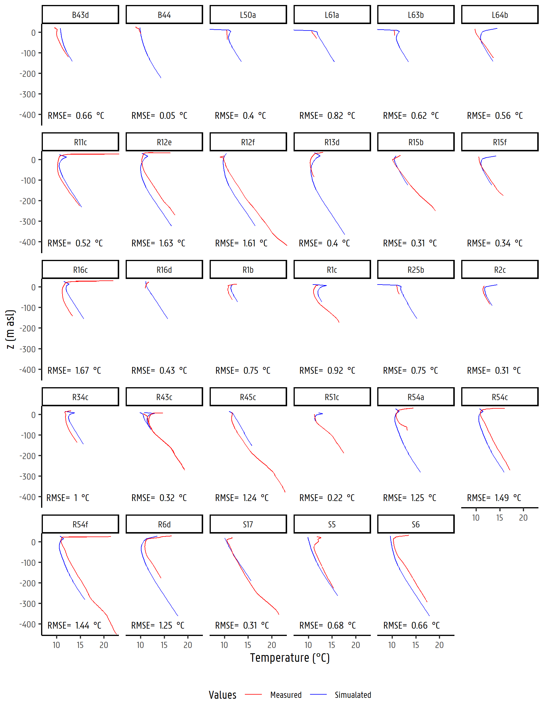
Figure A1Measured and simulated temperature–depth profiles for all locations across the Neogene Aquifer within the Nete catchment.
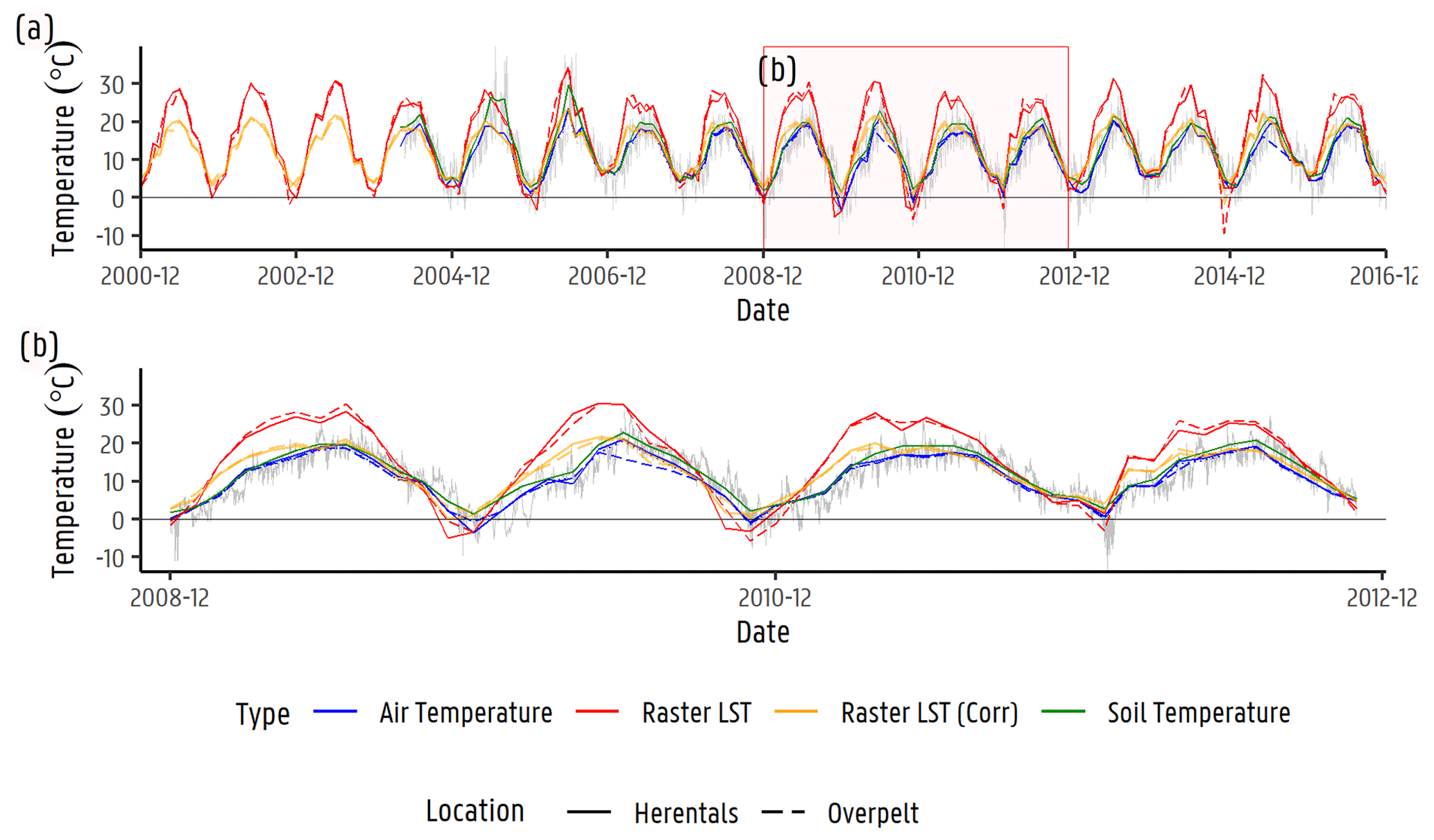
Figure A2(a) Temperature–time series of air and soil measured in different stations within and nearby the Nete catchment. Corresponding raw and corrected average land surface temperature (LST) based on remote sensing data are presented as well. (b) Inset of panel (a).
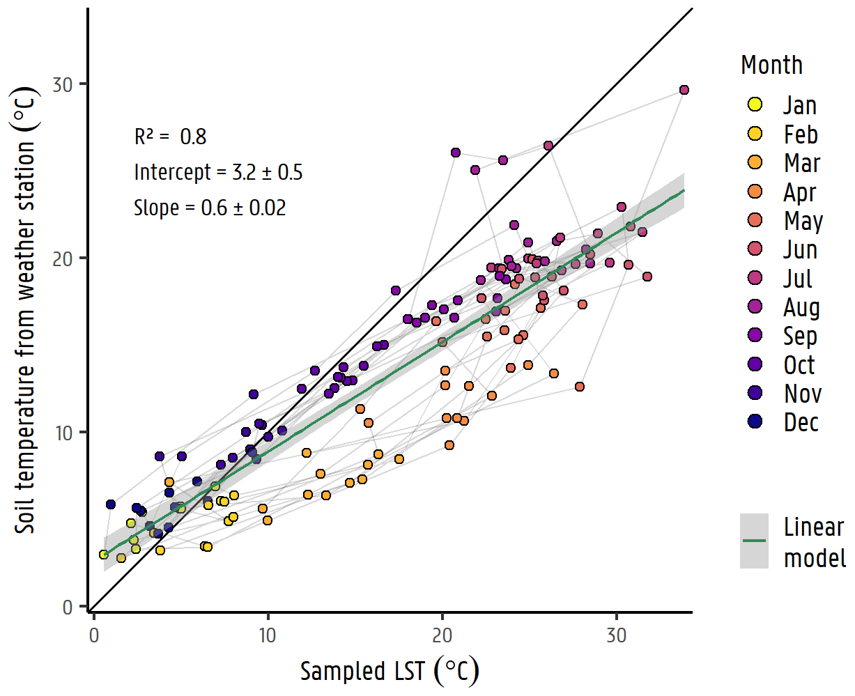
Figure A3In situ measurements at weather stations vs. sampled LST values. The linear model that was used to correct raster LST values is included.
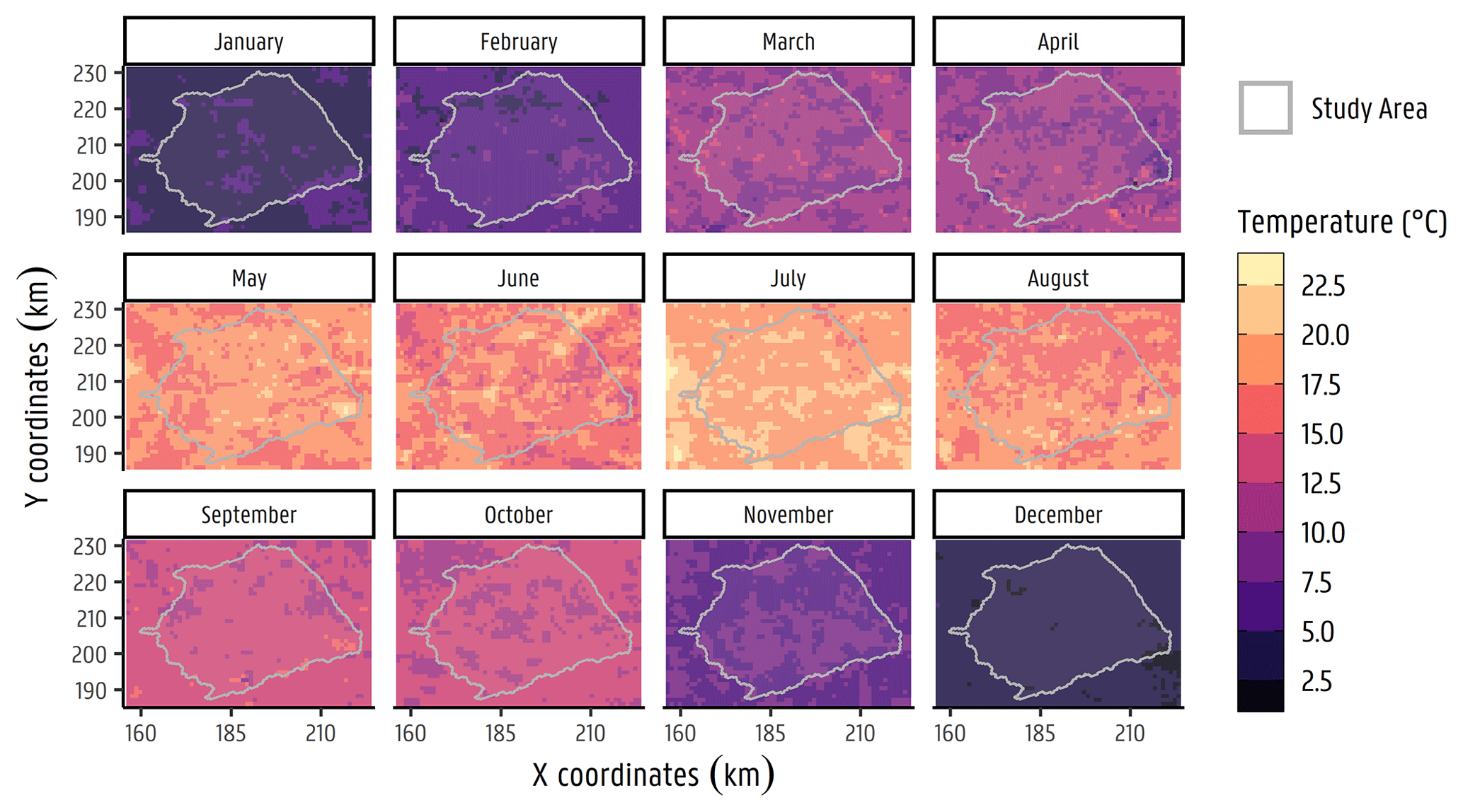
Figure A4Corrected MODIS monthly average LST with a 1 km resolution for the year 2001 within the Neogene Aquifer model (NAM) boundary.
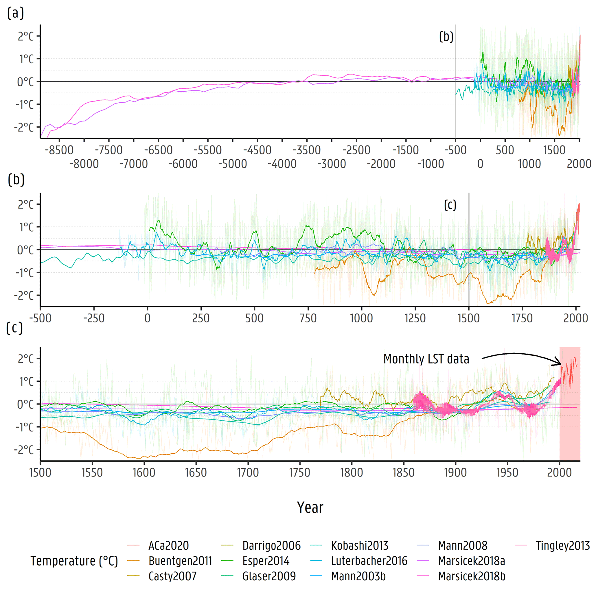
Figure A5Temperature–time curve for each author in the legend scaled to the 1961–1990 Belgian average for the past 10 519 years.

Figure A6Péclet numbers (Pe) derived from groundwater model results presented by Casillas-Trasvina et al. (2021). Note the considerably lower values (Pe≤1) in the deepest parts of the Neogene Aquifer corresponding to the Berchem and Voort sands.
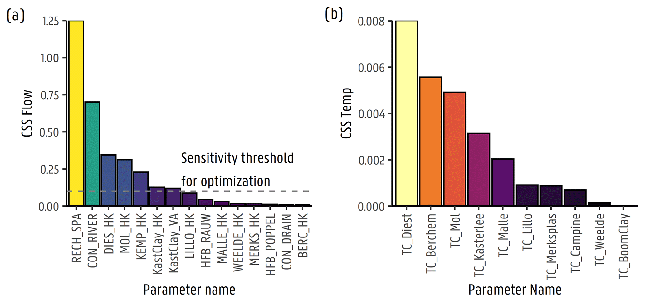
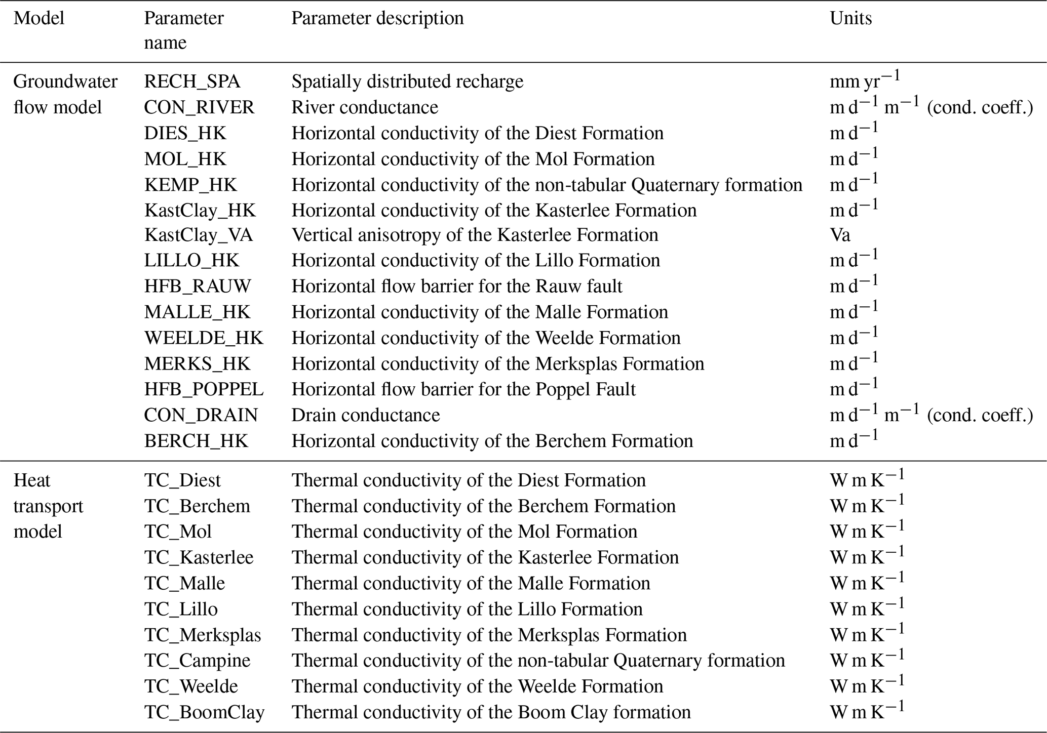
Figure A7Composite scaled sensitivities for (a) groundwater flow parameters, where HK means horizontal hydraulic conductivity for the hydrogeological formations, VA is vertical anisotropy, HFB and CON represent the hydraulic conductance for the horizontal flow barriers and drains, and (b) heat transport parameters, where TC means thermal conductivity for each hydrogeological formation.
Table A1Groundwater flow and transport models parameter names, as shown in Fig. A7.
Model codes and data are available upon request from the corresponding author.
ACT, BR, and KB designed the experiments and collected and processed data in different field campaigns. ACT carried the modelling experiments and performed simulations with contributions from BR. BR, KB, and KW provided supervision during the research period. LW (ONDRAF/NIRAS) provided part of the financial support and resources in this work. ACT prepared the paper, with contributions to writing, reviewing, and editing from all co-authors.
The contact author has declared that none of the authors has any competing interests.
Publisher's note: Copernicus Publications remains neutral with regard to jurisdictional claims in published maps and institutional affiliations.
This work has been performed in co-operation with, and with the financial support of, ONDRAF/NIRAS, the Belgian Agency for Radioactive Waste and Fissile Materials, and the SCK CEN Academy by SCK CEN, the Belgian nuclear research centre, as part of the programme on geological disposal of high-level/long-lived radioactive waste that is carried out by ONDRAF/NIRAS. The authors would like to acknowledge Victor Bense, for his advice and support during the first temperature–depth measurement campaign of 2019.
This research has been supported by NIRAS/ONDRAF and SCK CEN Academy in the framework of Alberto Casillas-Trasvina doctoral grant agreement.
This paper was edited by Monica Riva and reviewed by two anonymous referees.
Anderson, M. P.: Heat as a ground water tracer, Groundwater, 43, 951–968, https://doi.org/10.1111/j.1745-6584.2005.00052.x, 2005.
Bartsch, S., Frei, S., Ruidisch, M., Shope, C. L., Peiffer, S., Kim, B., and Fleckenstein, J. H.: River-aquifer exchange fluxes under monsoonal climate conditions, J. Hydrol., 509, 601–614, https://doi.org/10.1016/j.jhydrol.2013.12.005, 2014.
Bedekar, V., Morway, E., Langevin, C., and Tonkin, M.: MT3D-USGS version 1: A U.S. Geological Survey release of MT3DMS updated with new and expanded transport capabilities for use with MODFLOW, Tech. Meth., 84, US Geological Survey, https://doi.org/10.3133/tm6A53, 2016.
Beerten, K., Wemaere, I., Gedeon, M., Labat, S., Rogiers, B., Mallants, D., Salah, S., and Leterme, B.: Geological, hydrogeological, and hydrological data for the Dessel disposal site: Project near surface disposal of category A waste at Dessel, NIROND-TR 2009-05, https://www.researchgate.net/publication/248707737_Geological_hydrogeological_and_hydrological_data_for_the_Dessel_disposal_site (last access: 7 November 2022), January 2010.
Bense, V. F. and Person, M. A.: Faults as conduit-barrier systems to fluid flow in siliciclastic sedimentary aquifers, Water Resour. Res., 42, 1–18, https://doi.org/10.1029/2005WR004480, 2006.
Bense, V. F., Kurylyk, B. L., van Daal, J., van der Ploeg, M. J., and Carey, S. K.: Interpreting Repeated Temperature-Depth Profiles for Groundwater Flow, Water Resour. Res., 53, 8639–8647, https://doi.org/10.1002/2017WR021496, 2017.
Benz, S. A., Bayer, P., Blum, P., Hamamoto, H., Arimoto, H., and Taniguchi, M.: Comparing anthropogenic heat input and heat accumulation in the subsurface of Osaka, Japan, Sci. Total Environ., 643, 1127–1136, https://doi.org/10.1016/j.scitotenv.2018.06.253, 2018.
Bravo, H. R., Jiang, F., and Hunt, R. J.: Using groundwater temperature data to constrain parameter estimation in a groundwater flow model of a wetland system, Water Resour. Res., 38, 28-1–28-14, https://doi.org/10.1029/2000WR000172, 2002.
Buntgen, U., Tegel, W., Nicolussi, K., McCormick, M., Frank, D., Trouet, V., Kaplan, J. O., Herzig, F., Heussner, K.-U., Wanner, H., Luterbacher, J., and Esper, J.: 2500 Years of European Climate Variability and Human Susceptibility, Science, 331, 578–582, https://doi.org/10.1126/science.1197175, 2011.
Casillas-Trasvina, A. C., Rogiers, B., Beerten, K., Wouters, L., and Walraevens, K.: Exploring the hydrological effects of normal faults at the boundary of the Roer Valley Graben in Belgium using a catchment-scale groundwater flow model, Hydrogeol. J., 30, 133–149, https://doi.org/10.1007/s10040-021-02423-y, 2021.
Casty, C., Raible, C. C., Stocker, T. F., Wanner, H., and Luterbacher, J.: A European pattern climatology 1766–2000, Clim. Dynam., 29, 791–805, https://doi.org/10.1007/s00382-007-0257-6, 2007.
Chang, C.-M. and Yeh, H.-D.: Stochastic analysis of field-scale heat advection in heterogeneous aquifers, Hydrol. Earth Syst. Sci., 16, 641–648, https://doi.org/10.5194/hess-16-641-2012, 2012.
Chen, G. J., Sillen, X., Verstricht, J., and Li, X. L.: ATLAS III in situ heating test in boom clay: Field data, observation and interpretation, Comput. Geotech., 38, 683–696, https://doi.org/10.1016/j.compgeo.2011.04.001, 2011.
Clerc, M., Knight, N., Sousa, P., Barrett, J. L., and Atran, S.: Standard particle swarm optimisation, hal-00764996, HAL open science, https://hal.archives-ouvertes.fr/hal-00764996/document (last access: 7 November 2022), 2012.
Coetsiers, M. and Walraevens, K.: Chemical characterization of the Neogene Aquifer, Belgium, Hydrogeol. J., 14, 1556–1568, https://doi.org/10.1007/s10040-006-0053-0, 2006.
Coetsiers, M. and Walraevens, K.: The Neogene Aquifer, Flanders, Belgium, in: Nat. Groundw. Qual., chap. 12, Wiley, 263–286, https://doi.org/10.1002/9781444300345.ch12, 2008.
Constantz, J., Cox, M. H., and Su, G. W.: Comparison of Heat and Bromide as Ground Water Tracers Near Streams, Ground Water, 41, 647–656, https://doi.org/10.1111/j.1745-6584.2003.tb02403.x, 2003.
D'Arrigo, R., Mashig, E., Frank, D., Wilson, R., and Jacoby, G.: Temperature variability over the past millennium inferred from Northwestern Alaska tree rings, Clim. Dynam., 24, 227–236, https://doi.org/10.1007/s00382-004-0502-1, 2005.
D'Arrigo, R., Wilson, R., and Jacoby, G.: On the long-term context for late twentieth century warming, J. Geophys. Res., 111, D03103, https://doi.org/10.1029/2005JD006352, 2006.
Deckers, J., Van Noten, K., Schiltz, M., Lecocq, T., and Vanneste, K.: Integrated study on the topographic and shallow subsurface expression of the Grote Brogel Fault at the boundary of the Roer Valley Graben, Belgium, Tectonophysics, 722, 486–506, https://doi.org/10.1016/j.tecto.2017.11.019, 2018.
Deckers, J., De Koninck, R., Bos, S., Broothaers, M., Dirix, K., Hambsch, L., Lagrou, D., Lanckacker, T., Matthijs, J., Rombaut, B., Van Baelen, K., and Van Haren, T.: Geologisch (G3Dv3) en hydrogeologisch (H3D) 3D-lagenmodel van Vlaanderen, Studie uitgevoerd in opdracht van: Vlaams Planbureau voor Omgeving (Departement Omgeving) en Vlaamse Milieumaatschappij, Departement Omgeving, https://omgeving.vlaanderen.be/nl/geologisch-g3dv3-en-hydrogeologisch-h3d-3d-lagenmodel (last access: 7 November 2022), 2019.
Delsman, J. R., Winters, P., Vandenbohede, A., Oude Essink, G. H. P., and Lebbe, L.: Global sampling to assess the value of diverse observations in conditioning a real-world groundwater flow and transport model, Water Resour. Res., 52, 1652–1672, https://doi.org/10.1002/2014WR016476, 2016.
Delsman, J. R., Van Baaren, E. S., Siemon, B., Dabekaussen, W., Karaoulis, M. C., Pauw, P. S., Vermaas, T., Bootsma, H., De Louw, P. G. B., Gunnink, J. L., Wim Dubelaar, C., Menkovic, A., Steuer, A., Meyer, U., Revil, A., and Oude Essink, G. H. P.: Large-scale, probabilistic salinity mapping using airborne electromagnetics for groundwater management in Zeeland, the Netherlands, Environ. Res. Lett., 13, 1–12, https://doi.org/10.1088/1748-9326/aad19e, 2018.
Dentzer, J., Violette, S., Lopez, S., and Bruel, D.: Thermal anomalies and paleoclimatic diffusive and advective phenomena: example of the Anglo-Paris Basin, northern France, Hydrogeol. J., 25, 1951–1965, https://doi.org/10.1007/s10040-017-1592-2, 2017.
des Tombe, B. F., Bakker, M., Schaars, F., and van der Made, K. J.: Estimating Travel Time in Bank Filtration Systems from a Numerical Model Based on DTS Measurements, Groundwater, 56, 288–299, https://doi.org/10.1111/gwat.12581, 2018.
DiCiacca, A.: PhD Thesis: Spatially distributed recharge and groundwater – surface water interactions in groundwater models: from the field to the catchment scale, KU Leuven, https://kuleuven.limo.libis.be/discovery/fulldisplay?docid=lirias3271039&context=SearchWebhook&vid=32KUL_KUL:Lirias&search_scope=lirias_profile&tab=LIRIAS&adaptor=SearchWebhook&lang=en (last access: 7 November 2022), 2020.
Dong, L., Fu, C., Liu, J., and Wang, Y.: Disturbances of Temperature-Depth Profiles by Surface Warming and Groundwater Flow Convection in Kumamoto Plain, Japan, Geofluids, 2018, 15–18, https://doi.org/10.1155/2018/8451276, 2018.
Engelhardt, I., Prommer, H., Moore, C., Schulz, M., Schüth, C., and Ternes, T. A.: Suitability of temperature, hydraulic heads, and acesulfame to quantify wastewater-related fluxes in the hyporheic and riparian zone, Water Resour. Res., 49, 426–440, https://doi.org/10.1029/2012WR012604, 2013.
Esper, J., Düthorn, E., Krusic, P. J., Timonen, M., and Büntgen, U. L. F.: Northern European summer temperature variations over the Common Era from integrated tree-ring density records, J. Quatern. Sci., 29, 487–494, https://doi.org/10.1002/jqs.2726, 2014.
Fick, S. E. and Hijmans, R. J.: WorldClim 2: new 1-km spatial resolution climate surfaces for global land areas, Int. J. Climatol., 37, 4302–4315, https://doi.org/10.1002/joc.5086, 2017.
Freeze, R. A. and Cherry, J. A.: Groundwater, in: Vol. 7632, Prentice-Hall Inc., Englewood Cliffs, https://www.un-igrac.org/sites/default/files/resources/files/Groundwater book - English.pdf (last access: 7 November 2022), 1979.
Gedeon, M.: Neogene Aquifer Model, SCK-CEN external report ER-48, Report prepared by SCK⋅CEN in the framework of ONDRAF/NIRAS programme on geological disposal, 100 pp., https://www.researchgate.net/publication/27413017_Neogene_Aquifer_Model (last access: 7 November 2022), 2008.
Gedeon, M: Transport modelling in the Neogene Aquifer, Mol, Belgium, SCK-CEN external report ER-243, Report prepared by SCK⋅CEN in the framework of ONDRAF/NIRAS programme on geological disposal, https://publications.sckcen.be/portal/files/195734/ER-243.pdf (last access: 7 November 2022), 2015.
Glaser, R. and Riemann, D.: A thousand-year record of temperature variations for Germany and Central Europe based on documentary data, J. Quatern. Sci., 24, 437–449, https://doi.org/10.1002/jqs.1302, 2009.
Govaerts, J., Weetjens, E., and Beerten, K.: Numerical simulation of Permafrost Depth at the Mol site, https://www.researchgate.net/profile/Joan-Govaerts/publication/289377530_Numerical_simulation_of_permafrost_depth_at_the_Mol_site/links/568c121c08aeb488ea2fab1a/Numerical-simulation-of-permafrost-depth-at-the-Mol-site.pdf (last access: 7 November 2022), 2011.
Harbaugh, A. W.: MODFLOW-2005, The U.S. Geological Survey Ground-water Model, Ground-water Flow Process, USGS Tech. Methods 6-A16, USGS, 1–253, https://doi.org/10.3133/tm6A16, 2005.
Harbaugh, A. W., Banta, E., Hill, M. C., and Mcdonald, M. G.: MODFLOW-2005, The U.S. Geological Survey Modular Ground-Water Model – the Ground-Water Flow Process, US Geological Survey Techniques and Methods 6-A16, US Geological Survey, https://pubs.usgs.gov/tm/2005/tm6A16/PDF/TM6A16.pdf (last access: 7 November 2022), 2005.
Harris, R. N. and Chapman, D. S.: Stop-go temperature logging for precision applications, Geophysics, 72, E119–E123, https://doi.org/10.1190/1.2734382, 2007.
Hazaymeh, K. and Hassan, Q. K.: Fusion of MODIS and Landsat-8 surface temperature images: A new approach, PLoS One, 10, 1–13, https://doi.org/10.1371/journal.pone.0117755, 2015.
Hecht-Méndez, J., Molina-Giraldo, N., Blum, P., and Bayer, P.: Evaluating MT3DMS for heat transport simulation of closed geothermal systems, Ground Water, 48, 741–756, https://doi.org/10.1111/j.1745-6584.2010.00678.x, 2010.
Hidalgo, J. J., Carrera, J., and Dentz, M.: Steady state heat transport in 3D heterogeneous porous media, Adv. Water Resour., 32, 1206–1212, https://doi.org/10.1016/j.advwatres.2009.04.003, 2009.
Hoes, H., Reuss, M., Staudacher, L., and Mol, B.: The TESSAS Project in Mol: High Temperature Thermal Energy Storage in Saturated Sand Layers with Vertical Heat Exchangers and Thermal, in: Proceedings World Geothermal Congress 2005, 24–29 April 2005, Antalya, Turkey, https://www.geothermal-energy.org/pdf/IGAstandard/WGC/2005/1513.pdf (last access: 7 November 2022), 2005.
Irvine, D. J., Brunner, P., Franssen, H. H., and Simmons, C. T.: Heterogeneous or homogeneous? Implications of simplifying heterogeneous streambeds in models of losing streams, J. Hydrol., 424–425, 16–23, https://doi.org/10.1016/j.jhydrol.2011.11.051, 2012.
Irvine, D. J., Simmons, C. T., Werner, A. D., and Graf, T.: Heat and Solute Tracers: How Do They Compare in Heterogeneous Aquifers?, Groundwater, 53, 10–20, https://doi.org/10.1111/gwat.12146, 2015.
Irvine, D. J., Kurylyk, B. L., Cartwright, I., Bonham, M., Post, V. E. A., Banks, E. W., and Simmons, C. T.: Groundwater flow estimation using temperature-depth profiles in a complex environment and a changing climate, Sci. Total Environ., 574, 272–281, https://doi.org/10.1016/j.scitotenv.2016.08.212, 2017.
Jiang, Y. and Woodbury, A. D.: A full-Bayesian approach to the inverse problem for steady-state groundwater flow and heat transport, Geophys. J. Int., 167, 1501–1512, https://doi.org/10.1111/j.1365-246X.2006.03145.x, 2006.
Jones, P. D., New, M., Parker, D. E., Martin, S., and Rigor, I. G.: Surface air temperature and its changes over the past 150 years, Rev. Geophys., 37, 173–199, https://doi.org/10.1029/1999rg900002, 1999.
Jones, P. D., Lister, D. H., Osborn, T. J., Harpham, C., Salmon, M., and Morice, C. P.: Hemispheric and large-scale land-surface air temperature variations: An extensive revision and an update to 2010, J. Geophys. Res.-Atmos., 117, D05127, https://doi.org/10.1029/2011jd017139, 2012.
Kurtz, W., Hendricks Franssen, H.-J., Kaiser, H.-P., and Vereecken, H.: Joint assimilation of piezometric heads and groundwater temperatures for improved modeling of river-aquifer interactions, Water Resour. Res., 50, 1665–1688, https://doi.org/10.1002/2013WR014823, 2014.
Kurylyk, B. L., Irvine, D. J., and Bense, V. F.: Theory, tools, and multidisciplinary applications for tracing groundwater fluxes from temperature profiles, Wiley Interdisciplin. Rev. Water, 6, e1329, https://doi.org/10.1002/wat2.1329, 2018.
Laga, P., Louwye, S., and Geets, S.: Paleogene and Neogene lithostratigraphic units (Belgium), Geol. Belgica, 4, 135–152, 2001.
Langevin, C. D., Thorne, D. T., Dausman, A. M., Sukop, M. C., and Guo, W.: SEAWAT Version 4: A Computer Program for Simulation of Multi-Species Solute and Heat Transport, USGS Tech. B.6, Series number 6-A22, USGS, 39 pp. https://doi.org/10.3133/tm6A22, 2008.
Langevin, C. D., Hughes, J. D., Banta, E. R., Niswonger, R. G., Panday, S., and Provost, A. M.: Documentation for the MODFLOW 6 Groundwater Flow Model, Techniques and Methods 6-A55, USGS, https://doi.org/10.3133/tm6A55, 2017.
Lavielle, M.: Detection of multiple changes in a sequence of dependent variables, Stoch. Process. Appl., 83, 79–102, https://doi.org/10.1016/S0304-4149(99)00023-X, 1999.
Lavielle, M.: Using penalized contrasts for the change-point problem, Signal Process., 85, 1501–1510, https://doi.org/10.1016/j.sigpro.2005.01.012, 2005.
Leterme, B. and Mallants, D.: Simulation of evapotranspiration and groundwater recharge in the Nete catchment accouting for different land cover types and for present and future climate conditions, https://www.researchgate.net/publication/258342433_Simulation_of_evapotranspiration_and_groundwater_recharge_in_the_Nete_catchment_accounting_for_different_land_cover_types_and_for_present_and_future_climate_conditions (last access: 7 November 2022), 2012.
Liu, S., Zhou, Y., Kamps, P., Smits, F., and Olsthoorn, T.: Effect of temperature variations on the travel time of infiltrating water in the Amsterdam Water Supply Dunes (the Netherlands), Hydrogeol. J., 27, 2199–2209, https://doi.org/10.1007/s10040-019-01976-3, 2019.
Ljungqvist, F. C., Seim, A., Krusic, P. J., González-Rouco, J. F., Werner, J. P., Cook, E. R., Zorita, E., Luterbacher, J., Xoplaki, E., Destouni, G., García-Bustamante, E., Aguilar, C. A. M., Seftigen, K., Wang, J., Gagen, M. H., Esper, J., Solomina, O., Fleitmann, D., and Büntgen, U.: European warm-season temperature and hydroclimate since 850 CE, Environ. Res. Lett., 14, 84015, https://doi.org/10.1088/1748-9326/ab2c7e, 2019.
Luterbacher, J., Werner, J. P., Smerdon, J. E., Fernández-Donado, L., González-Rouco, F. J., Barriopedro, D., Ljungqvist, F. C., Büntgen, U., Zorita, E., Wagner, S., Esper, J., McCarroll, D., Toreti, A., Frank, D., Jungclaus, J. H., Barriendos, M., Bertolin, C., Bothe, O., Brázdil, R., Camuffo, D., Dobrovolný, P., Gagen, M., García-Bustamante, E., Ge, Q., Gómez-Navarro, J. J., Guiot, J., Hao, Z., Hegerl, G. C., Holmgren, K., Klimenko, V. V, Martín-Chivelet, J., Pfister, C., Roberts, N., Schindler, A., Schurer, A., Solomina, O., von Gunten, L., Wahl, E., Wanner, H., Wetter, O., Xoplaki, E., Yuan, N., Zanchettin, D., Zhang, H., and Zerefos, C.: European summer temperatures since Roman times, Environ. Res. Lett., 11, 24001, https://doi.org/10.1088/1748-9326/11/2/024001, 2016.
Ma, R., Zheng, C., Zachara, J. M., and Tonkin, M.: Utility of bromide and heat tracers for aquifer characterization affected by highly transient flow conditions, Water Resour. Res., 48, 1–18, https://doi.org/10.1029/2011WR011281, 2012.
Majorowicz, J. A. and Grasby, S. E.: Geothermics Heat transition for major communities supported by geothermal energy development of the Alberta Basin, Canada, Geothermics, 88, 101883, https://doi.org/10.1016/j.geothermics.2020.101883, 2020.
Mallants, D.: A long-term solution for Belgian category A waste: SCKCEN provides scientific input for thesurface disposal facility in Dessel (INIS-BE–0014), SCK-CEN Tech. Rep. 43, 50–51, https://inis.iaea.org/collection/NCLCollectionStore/_Public/43/095/43095133.pdf?r=1 (last access: 7 November 2022), 2010.
Mann, M. E.: Encyclopedia of Global Environmental Change, in: Vol 1: The Earth system: physical and chemical dimensions of global environmental change – Little Ice Age, edited by: Michael, T. M., MacCracken, C., and Perry, J., John Wiley & Sons, ISBN 978-0-470-85360-3, 2002.
Mann, M. E., Zhang, Z., Rutherford, S., Bradley, R. S., Hughes, M. K., Shindell, D., Ammann, C., Faluvegi, G., and Ni, F.: Global Signatures and Dynamical Origins of the Little Ice Age and Medieval Climate Anomaly, Science, 326, 1256–1260, https://doi.org/10.1126/science.1177303, 2009.
Marsicek, J., Shuman, B. N., Bartlein, P. J., Shafer, S. L., and Brewer, S.: Reconciling divergent trends and millennial variations in Holocene temperatures, Nature, 554, 92–96, https://doi.org/10.1038/nature25464, 2018.
Marty, N. C. M., Hamm, V., Castillo, C., Thiéry, D., and Kervévan, C.: Geothermics Modelling water-rock interactions due to long-term cooled-brine reinjection in the Dogger carbonate aquifer (Paris basin) based on in-situ geothermal well data, Geothermics, 88, 101899, https://doi.org/10.1016/j.geothermics.2020.101899, 2020.
Masbruch, M. D., Gardner, P. M., and Brooks, L. E.: Hydrology and Numerical Simulation of Groundwater Movement and Heat Transport in Snake Valley and Surrounding Areas, Juab, Millard, and Beaver Counties, Utah, and White Pine and Lincoln Counties, Nevada, Scientific Investigations Report 2014-5103, USGS, https://doi.org/10.3133/sir20145103, 2014.
Mazurek, M., Alt-Epping, P., Bath, A., Gimmi, T., and Waber, H. N.: Natural Tracer Profiles Across Argillaceous Formations: The CLAYTRAC Project, Organ. Econ. Co-operation Dev., 6253, 251–265, 2009.
Mullen, K., Ardia, D., Gil, D., Windover, D., and Cline, J.: DEoptim: An R Package for Global Optimization by Differential Evolution, J. Stat. Softw., 40, 1–26, https://doi.org/10.18637/jss.v040.i06, 2011.
Munz, M., Oswald, S. E., and Schmidt, C.: Coupled Long-Term Simulation of Reach-Scale Water and Heat Fluxes Across the River-Groundwater Interface for Retrieving Hyporheic Residence Times and Temperature Dynamics, Water Resour. Res., 53, 8900–8924, https://doi.org/10.1002/2017WR020667, 2017.
ONDRAF/NIRAS: The cAt project in Dessel: A long-term solution for Belgian category A waste, Report NIROND 2010-02 E, 144 pp., https://www.stora.org/sites/stora.org/files/cAt_masterplanENG_low.pdf (last access: 7 November 2022), 2010.
ONDRAF/NIRAS: ONDRAF/NIRAS Research, Development and Demonstration (RD&D) Plan for the geological disposal of high-level and/or long-lived radioactive waste, Belgian Agency Radioact, Waste Enriched Fissile Mater, Report, NIROND-TR 2013-12 E 413, https://www.ondraf.be/sites/default/files/2020-05/ONDRAFNIRAS (last access: 8 November 2022), 2013.
Patyn, J., Ledoux, E., and Bonne, A.: Geohydrological research in relation to radioactive waste disposal in an argillaceous formation, J. Hydrol., 109, 267–285, https://doi.org/10.1016/0022-1694(89)90019-X, 1989.
Person, M., Raffensperger, J. P., Ge, S., and Garven, G.: Basin-scale hydrogeologic modeling, Rev. Geophys., 34, 61–87, https://doi.org/10.1029/95RG03286, 1996.
Pollack, H. N., Hurter, S. J., and Johnson, J. R.: Heat flow from the Earth's interior: Analysis of the global data set, Rev. Geophys., 31, 267–280, https://doi.org/10.1029/93RG01249, 1993.
Rau, G. C., Andersen, M. S., McCallum, A. M., and Acworth, R. I.: Analytical methods that use natural heat as a tracer to quantify surface water-groundwater exchange, evaluated using field temperature records, Hydrogeol. J., 18, 1093–1110, https://doi.org/10.1007/s10040-010-0586-0, 2010.
R Core Team: R: A Language and Environment for Statistical Computing, https://www.r-project.org/ (last access: 7 November 2022), 2020.
Read, T., Bour, O., Bense, V., Le Borgne, T., Goderniaux, P., Klepikova, M. V., Hochreutener, R., Lavenant, N., and Boschero, V.: Characterizing groundwater flow and heat transport in fractured rock using fiber-optic distributed temperature sensing, Geophys. Res. Lett., 40, 2055–2059, https://doi.org/10.1002/grl.50397, 2013.
Reinart, A. and Reinhold, M.: Mapping surface temperature in large lakes with MODIS data, Remote Sens. Environ., 112, 603–611, https://doi.org/10.1016/j.rse.2007.05.015, 2008.
Rodríguez-Escales, P., Barba, C., Sanchez-Vila, X., Jacques, D., and Folch, A.: Coupling Flow, Heat, and Reactive Transport Modeling to Reproduce in Situ Redox Potential Evolution: Application to an Infiltration Pond, Environ. Sci. Technol., 54, 12092–12101, https://doi.org/10.1021/acs.est.0c03056, 2020.
Rogiers, B.: Exploratory temperature logging in the upper part of the Neogene aquifer at Mol-Dessel-Retie, SCK⋅CEN external report ER-258, https://publications.sckcen.be/portal/files/250487/ER-258.pdf (last access: 7 November 2022), 2014.
Rogiers, B.: Groundwater flow and solute transport modelling from within R: Development of the RMODFLOW and RMT3DMS packages, in: Geophysical Research Abstracts 17: EGU General Assembly 2015-11879, 12–17 April 2015, Vienna, Austria, https://meetingorganizer.copernicus.org/EGU2015/EGU2015-11879.pdf (last access: 7 November 2022), 2015.
Rogiers, B.: RMODFLOW: Pre- and post-processing of MODFLOW files in R, GitHub [code], https://github.com/rogiersbart/RMODFLOW (last access: 7 November 2022), 2016a.
Rogiers, B.: RMT3DMS: Pre- and post-processing of MT3DMS files, GitHub [code], https://github.com/rogiersbart/RMT3DMS (last access: 7 November 2022), 2016b.
Rogiers, B., Beerten, K., Smeekens, T., Mallants, D., Gedeon, M., Huysmans, M., Batelaan, O., and Dassargues, A.: Derivation of flow and transport parameters from outcropping sediments of the neogene aquifer, Belgium, Geol. Belgica, 16, 129–147, 2013.
Rogiers, B., Vienken, T., Gedeon, M., Batelaan, O., Mallants, D., Huysmans, M., and Dassargues, A.: Multi-scale aquifer characterization and groundwater flow model parameterization using direct push technologies, Environ. Earth Sci., 72, 1303–1324, https://doi.org/10.1007/s12665-014-3416-1, 2014.
Rogiers, B., Labat, S., and Gedeon, M.: An assessment of dilution tests and ambient temperature logging for quantifying groundwater flow in the Neogene aquifer, https://publications.sckcen.be/portal/files/4577567/An_assessment_of_dilution_tests_and_ambient_temperature_logging_for_quantifying_groundwater_flow_in_the_Neogene_aquifer.pdf (last access: 7 November 2022), 2015.
Saar, M. O.: Review: Geothermal heat as a tracer of large-scale groundwater flow and as a means to determine permeability fields, Hydrogeol. J., 19, 31–52, https://doi.org/10.1007/s10040-010-0657-2, 2011.
Schilling, O. S., Cook, P. G., and Brunner, P.: Beyond Classical Observations in Hydrogeology: The Advantages of Including Exchange Flux, Temperature, Tracer Concentration, Residence Time, and Soil Moisture Observations in Groundwater Model Calibration, Rev. Geophys., 57, 146–182, https://doi.org/10.1029/2018RG000619, 2019.
Shanafield, M. and Cook, P. G.: Transmission losses, infiltration and groundwater recharge through ephemeral and intermittent streambeds: A review of applied methods, J. Hydrol., 511, 518–529, https://doi.org/10.1016/j.jhydrol.2014.01.068, 2014.
Sippel, J., Fuchs, S., Cacace, M., Braatz, A., Kastner, O., Huenges, E., and Scheck-Wenderoth, M.: Deep 3D thermal modelling for the city of Berlin (Germany), Environ. Earth Sci., 70, 3545–3566, https://doi.org/10.1007/s12665-013-2679-2, 2013.
Smith, D. C. and Elmore, A. C.: Geothermics Characterizing lithological effects on large scale borehole heat exchangers during cyclic heating of the subsurface, Geothermics, 77, 166–174, https://doi.org/10.1016/j.geothermics.2018.09.008, 2019.
Tingley, M. P. and Huybers, P.: Recent temperature extremes at high northern latitudes unprecedented in the past 600 years, Nature, 496, 201–205, https://doi.org/10.1038/nature11969, 2013.
Tomlinson, C. J., Chapman, L., Thornes, J. E., and Baker, C.: Remote sensing land surface temperature for meteorology and climatology: A review, Meteorol. Appl., 18, 296–306, https://doi.org/10.1002/met.287, 2011.
Trefry, M. G. and Muffels, C.: FEFLOW: A finite-element ground water flow and transport modeling tool, Ground Water, 45, 525–528, https://doi.org/10.1111/j.1745-6584.2007.00358.x, 2007.
Vandenberghe, N., De Craen, M., and Wouters, L.: The Boom Clay Geology from sedimentation to present-day occurrence – a review, Mem. Geol. Surv. Belgium, 60, 76 pp., http://biblio.naturalsciences.be/rbins-publications/memoirs-of-the-geological-survey-of-belgium/pdfs/msgb-2014-60.pdf (last access: 7 November 2022), 2014.
Vandersteen, K., Gedeon, M., and De Craen, M.: Solute Transport in Boom Clay, External report SCK⋅CEN-ER-237, https://publications.sckcen.be/portal/files/320701/ER-237.pdf (last access: 7 November 2022), 2013.
Van Keer, I., Marivoet, J., Wemaere, I., Hardy, L., and Labat, S.: A PalaeoHYdrogeological study of the MOL site: PHYMOL. An EC 4th Framework Project Nuclear Safety (1997–1999), CEA/DCC/DE FI4W-CT96-0026, 113 pp., 1999.
van Lysebetten, G., Huybrechts, N., and Francois, L.: Geschiktheidskaarten Geothermie. Thermische Geleidbaarheid Ondergrond Vlaanderen, Databank Onderground Vlaanderen [data set], https://www.dov.vlaanderen.be/geonetwork/srv/api/records/285875a7-7d18-4b93-95f1-df8c4a7bddcc (last access: 7 November 2022), 2013.
Vanneste, K., Camelbeeck, T., and Verbeeck, K.: Model of composite seismic sources for the Lower Rhine Graben, northwest Europe, Bull. Seismol. Soc. Am., 103, 984–1007, https://doi.org/10.1785/0120120037, 2013.
Verbeeck, K., Wouters, L., Vanneste, K., Camelbeeck, T., Vandenberghe, D., Beerten, K., Rogiers, B., Schiltz, M., Burow, C., Mees, F., De Grave, J., and Vandenberghe, N.: Episodic activity of a dormant fault in tectonically stable Europe: The Rauw fault (NE Belgium), Tectonophysics, 699, 146–163, https://doi.org/10.1016/j.tecto.2017.01.023, 2017.
Voss, C. I. and Provost, A.: Version of September 22, 2010 (SUTRA Version 2.2), USGS Water Resour. Investig. Rep. 02-4231, USGS, https://water.usgs.gov/water-resources/software/sutra/ReleaseNotes_SUTRA_2_2.pdf (last access: 7 November 2022), 2010.
Wan, Z., Zhang, Y., Zhang, Q., and Li, Z. liang: Validation of the land-surface temperature products retrieved from terra moderate resolution imaging spectroradiometer data, Remote Sens. Environ., 83, 163–180, https://doi.org/10.1016/S0034-4257(02)00093-7, 2002.
Yu, L., Rogiers, B., Gedeon, M., Marivoet, J., De Craen, M., and Mallants, D.: A critical review of laboratory and in-situ hydraulic conductivity measurements for the Boom Clay in Belgium, Appl. Clay Sci., 75–76, 1–12, https://doi.org/10.1016/j.clay.2013.02.018, 2013.
Zambrano-Bigiarini, M. and Rojas, R.: A model-independent Particle Swarm Optimisation software for model calibration, Environ. Model. Softw., 43, 25, https://doi.org/10.1016/j.envsoft.2013.01.004, 2013.
Zambrano-Bigiarini, M., Clerc, M., and Rojas, R.: Standard Particle Swarm Optimisation 2011 at CEC-2013: A baseline for future PSO improvements, in: 2013 IEEE Congress on Evolutionary Computation, 20–23 June 2013, Cancun, Mexico, https://doi.org/10.1109/CEC.2013.6557848, 2013.
Zheng, C.: MT3DMS v5.3 Supplemental User's Guide Technical Report, Deparment of Geological Sciences, The University of Alabama, Tyscakiisa, Alabama, 56 pp., https://hydro.geo.ua.edu/mt3d/mt3dms_v5_supplemental.pdf (last access: 7 November 2022), 2010.