Using machine learning to predict optimal electromagnetic induction instrument configurations for characterizing the shallow subsurface

Electromagnetic induction (EMI) is used widely for hydrological and other environmental studies. The apparent electrical conductivity (EC_a), which can be mapped efficiently with EMI, correlates with a variety of important soil attributes. EMI instruments exist with several configurations of coil spacing, orientation, and height. There are general, rule-of-thumb guides to choose an optimal instrument configuration for a specific survey. The goal of this study was to provide a robust and efficient way to design this optimization task. In this investigation, we used machine learning (ML) as an efficient tool for interpolating among the results of many forward model runs. Specifically, we generated an ensemble of 100 000 EMI forward models representing the responses of many EMI configurations to a range of three-layer subsurface models. We split the results into training and testing subsets and trained a decision tree (DT) with gradient boosting (GB) to predict the subsurface properties (layer thicknesses and EC values). We further examined the value of prior knowledge that could limit the ranges of some of the soil model parameters. We made use of the intrinsic feature importance measures of machine learning algorithms to identify optimal EMI designs for specific subsurface parameters. The optimal designs identified using this approach agreed with those that are generally recognized as optimal by informed experts for standard survey goals, giving confidence in the ML-based approach. The approach also offered insight that would be difficult, if not impossible, to offer based on rule-of-thumb optimization. We contend that such ML-informed design approaches could be applied broadly to other survey design challenges.

1 Introduction

Water movement through the vadose zone is often controlled by the near-surface layering of soil. In the simplest sense, this is often represented as a small number of horizontal layers, such as is often related to soil formation processes leading to distinct soil layers. The hydrogeologic structure places critical controls on processes ranging from infiltration to percolation to root water uptake to recharge, thereby playing a critical role in most hydrologic systems (Winter et al., 1998; Nimmo, 2009). The need to describe this shallow hydrogeologic structure has been a major driver in the development and adoption of hydrogeophysical methods (Binley et al., 2015).

Electromagnetic induction (EMI) is a noncontact method to measure the apparent electrical conductivity (EC_a) of the shallow subsurface. The EC_a is an integration of the electrical conductivity of all layers in the subsurface. EMI works when a transmitter coil produces an electromagnetic field that induces secondary currents in the subsurface soils. The combined current is measured with a receiver coil (Nabighian and Macnae, 1991). The strength of the measured field is used to estimate the EC_a within the sample volume of the measurement (Doolittle and Brevik, 2014). EMI instruments differ in the orientations of their coils: some use transmitter and receiver coils that have their long axis horizontal with respect to the ground surface (HCP), others orient both coils vertically (VCP), and some use one horizontal and one vertical coil in a perpendicular arrangement (PRP). In addition, instruments differ in the separation of the coils, with larger separations used to measure to greater depth. Finally, an operator can choose different instrument heights above ground, which also impact the spatial sensitivity of the measurement in the subsurface. We refer to the collective choices of coil orientation, separation, and height above ground as the instrument configuration.

For several decades, EMI instruments have been used to gather measurements of EC_a of the soil. The EC_a of soil is positively correlated with salinity, water content, and clay content (Doolittle and Brevik, 2014). As a result, EC_a is a meaningful (but complex) aggregate measure of soil properties (Palacky, 2011). Because the EMI method is noncontact, it is reasonably fast and inexpensive compared with direct soil sampling, resulting in a frequent use in agriculture (McCutcheon et al., 2006; Daccache et al., 2015; Adhikari and Hartemink, 2017), soil mapping (James et al., 2003; Cockx et al., 2009; Heil and Schmidhalter, 2012; Reyes et al., 2018), and archeological investigations (Saey et al., 2013, 2015; De Smedt et al., 2014; Christiansen et al., 2016). In addition to the challenges introduced by EC_a being sensitive to multiple soil properties, quantitative interpretation of EMI measurements is complicated by the complex averaging of the local soil EC within the instrument's sample volume. (Note that we use the term EC to refer to the actual bulk electrical conductivity of a soil, which may vary within the measurement volume of the instrument, and we use EC_a to refer to the average EC that is measured from EMI instrument responses.) More challenging still, the spatial sensitivity (or spatial weighting) of the EC depends on the instrument configuration (McNeill, 1980). Finally, in some cases, the spatial sensitivity may have a higher dependency on the absolute value and spatial distribution of the EC (Callegary et al., 2012).

In this investigation, we avoid the common assumption that the spatial sensitivity only depends on the instrument configuration, but we consider a complete forward model of EMI response. The spatial averaging of EMI is not an issue if the medium is electrically homogeneous. However, most soils have some structure – at a minimum, agricultural soils display horizontal layering with a distinct uppermost layer (the Ap horizon). Therefore, the optimal design of an EMI configuration should select the orientation, separation, and height of the coils to locate the instrument sensitivity in the subsurface to best determine the subsurface properties. The depth of investigation (DOI) of EMI instruments is, both in the scientific literature (Saey et al., 2009a, b, 2012; De Smedt et al., 2014; Doolittle and Brevik, 2014; Adamchuk et al., 2015) and by the manufacturers (Dualem Inc., Canada), often estimated to be at the depth that has 70 % of the cumulative response. There is a relationship between the depth sensitivity of the instrument response and the coil spacing and position. Therefore, in practice, the 70 % cumulative response rule is frequently converted to a rule of thumb that states that larger coil spacings and HCP should be used for deeper investigations, whereas short spacing and VCP or PRP should be used for shallow investigation (Acworth, 1999; Beamish, 2011; Cockx et al., 2009; Heil and Schmidhalter, 2015, 2019). While this rule of thumb is not wrong, the terms shallow and deep are subjective and will have different meaning depending on whether it is a hydrogeologist, archeologist, agronomist, or a geophysicist who applies the terms. It also fails to make any distinction between using the VCP or PRP coil orientation. These basic guides become more difficult if the objective is to determine subsurface properties in a nonhomogeneous medium, even a simple layered case. For these conditions, the advice is to use multiple coils with some combination of orientation, separation, and height. Nevertheless, little specific guidance is offered. Furthermore, the rule of thumb offers no way to consider the possible impact of prior knowledge (e.g., bounds on the expected depth of the topmost layer) in the survey design. Commercially available EMI instruments for relatively shallow applications offer a wide range of designs based on differences in the three instrument characteristics. This makes it difficult to make an informed choice regarding the preferred instrument and configuration.

Aside from the generally applied rule of thumb and sensitivity analysis there are several published efforts to optimize the design of geophysical surveys (e.g., Furman et al., 2007; Khodja et al., 2010; Song et al., 2016). These methods seek to estimate the reduction in prediction uncertainty based on changes in experiment design through inverse modeling. Applying these design optimization approaches to EMI would require that the responses of many configurations be computed for multiple soil models. Each survey design includes multiple measurements at each location, each with a different configuration, that jointly provide the most useful information for inferring specific, user-identified subsurface properties; that is, a user is faced with the question of which combination of configurations is optimal given their measurement priorities and, ideally, incorporating any applicable constraints that they may have regarding the subsurface conditions. Any method that requires formal inversion of each proposed combination of configurations is computationally expensive.

Machine learning (ML) describes a wide range of regression algorithms used for pattern recognition. ML has grown in popularity and is now used regularly within and beyond science. The simplest ML tools are based on decision trees (DT), which are supervised ML techniques that perform classification or regression based on observations. DTs are computationally inexpensive, but they can have limited predictive skill (Hastie et al., 2001). To improve their performance, DTs are often augmented by ensemble learning methods such as bagging (Breiman, 1996) and boosting (Friedman, 2001). The ML approach is different from traditional inverse modeling because ML is trained to balance generalization with goodness of fit. A sensitivity or inverse model approach would have to be repeated multiple times for each subset to estimate the value of every instrument configuration. The feature importance of tree-based ML gives a data value analysis at each step of the ML training procedure without extra effort. This makes the ML approach very efficient for calculating the information content of instrument configurations for an ensemble of soils compared with the inverse analysis of the data value.

One of the challenges of both scientific and environmental investigations is to determine the optimal data to acquire; these data are often used to either provide structural information or constrain model parameterization. Measurement optimization is an attempt to balance data quality and the work expended in the field and laboratory. The ultimate goal is to develop an efficient and robust approach to measurement optimization, with the hope that a similar approach could be extended into other measurement network design problems. The specific objective of this investigation was to present the approach in combination with a simple geophysical model to select sets of EMI configurations that are optimal given the specific survey goals and any independent knowledge of the subsurface electrical properties.

2 Theory

Depth sensitivity of EMI instruments

If the subsurface is electrically homogeneous within the sample volume of the instrument, the EMI instrument response (EC_a) can be related directly to the EC of the subsurface. In almost all subsurface media, the EC varies with depth due to soil layering. For these conditions, multiple measurements, made using different coil spacing and separations, can be interpreted simultaneously to infer the EC profile. This requires a model of the depth sensitivity of the EMI measurement.

We apply the Maxwell-based full solutions (Eqs. 1, 2, and 3) from Wait (1982) to calculate the relationship Q between the secondary field (H_s) and the primary field (H_p). The solution works for a one-dimensional subsurface, and it is valid for low frequencies because it assumes that the electromagnetic fields spread due to conduction currents:

$$\begin{array}{}\text{(1)}& {\displaystyle }& {\displaystyle }{Q}_{\text{VCP}}=\text{Im}{\left({\displaystyle \frac{H_{\mathrm{S}}}{H_{\mathrm{P}}}}\right)}_{\text{VCP}}=\text{Im}\left(-s^{\mathrm{2}}\underset{\mathrm{0}}{\overset{\mathrm{\infty }}{\int }}{R}_{\mathrm{0}}{J}_{\mathrm{1}}\left(s\mathit{\lambda }\right)\mathit{\lambda }\mathrm{d}\mathit{\lambda }\right),\text{(2)}& {\displaystyle }& {\displaystyle }{Q}_{\text{HCP}}=\text{Im}{\left({\displaystyle \frac{H_{\mathrm{S}}}{H_{\mathrm{P}}}}\right)}_{\text{HCP}}=\text{Im}\left(-s^{\mathrm{3}}\underset{\mathrm{0}}{\overset{\mathrm{\infty }}{\int }}{R}_{\mathrm{0}}{J}_{\mathrm{0}}\left(s\mathit{\lambda }\right){\mathit{\lambda }}^{\mathrm{2}}\mathrm{d}\mathit{\lambda }\right),\text{(3)}& {\displaystyle }& {\displaystyle }{Q}_{\text{PRP}}=\text{Im}{\left({\displaystyle \frac{H_{\mathrm{S}}}{H_{\mathrm{P}}}}\right)}_{\text{PRP}}=\text{Im}\left(-s^{\mathrm{3}}\underset{\mathrm{0}}{\overset{\mathrm{\infty }}{\int }}{R}_{\mathrm{0}}{J}_{\mathrm{1}}\left(s\mathit{\lambda }\right){\mathit{\lambda }}^{\mathrm{2}}\mathrm{d}\mathit{\lambda }\right),\end{array}$$

where Im means that only the imaginary component is considered; R₀ is an interlayer reflection factor; J₀ and J₁ are Bessel functions of the zeroth and first orders, respectively; and λ is the radial wave number. The integrals of Eqs. (1), (2), and (3) represent Hankel transforms, and these are calculated with linear filtering (Anderson, 1979; Guptasarma and Singh, 1997) in the EMagPy software (McLachlan et al., 2020). The low induction number (LIN) approximation proposed by McNeil (1980) assumes that depth of investigation does not depend on the EC of the subsurface. Therefore, a method similar to that of von Hebel et al. (2019) is used through EMagPy (McLachlan et al., 2020) to estimate EC_a from Q. The EC_a is estimated by minimizing the differences between a predicted or measured Q_pred and a Q value calculated for an equal homogenous half-space, Q_homo. The minimized difference approach is valid for a broader range of EC_a compared with the LIN approximation (von Hebel et al., 2019; McLachlan et al., 2020). We refer to von Hebel et al. (2019) for a more detailed description of this method.

Many efforts have been made to create geophysical modeling tools (Monteiro Santos, 2004; Auken et al., 2015; Saey et al., 2016). However, EMagPy (McLachlan et al., 2020) offers the user the opportunity to use several models and makes them readily available to a wide audience, as it is an open-source software. This study uses a complete forward model when estimating EC_a, but there is no hindrance to use a simpler geophysical model or a model describing a different process.

3 Materials and methods

In this study, we describe a specific EMI instrument configuration based on the three coil orientations, horizontal (HCP), vertical (VCP), and perpendicular (PRP); coil separation (in m); and instrument height (in m). For example, a configuration that uses coils that are horizontal to the surface with a separation of 1 m and an instrument height of 0.3 m would be named: “HCP_1.0_0.3”. The EC of any layer is an actual electrical property of that specific medium, and it is referred to as “EC” followed by the layer name. For example, the EC of the A layer is referred to as “ECA”. Likewise, the thickness of any layer is denoted by “Thick” followed by the layer name; thus, the thickness of the A layer is denoted as “ThickA”. All symbols and abbreviations can be found in Appendix A.

3.1 Generating the model ensemble

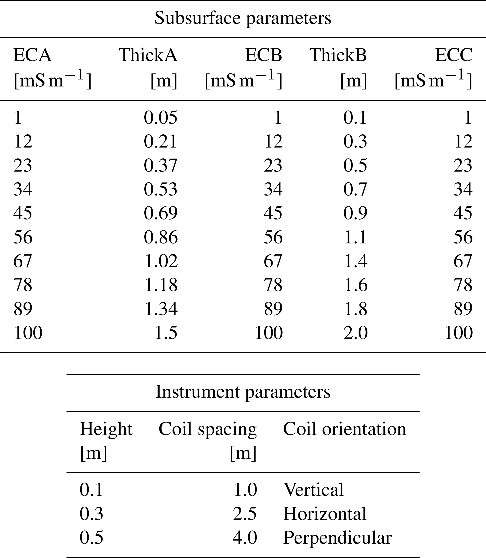
We consider a three-layer soil profile, which is common for agricultural soils with distinctly developed A, B, and C layers characterizing changes in the physical, chemical, and biological characteristics with depth (Fig. 1). Electrical properties are assumed to be constant horizontally within the sample volume of the instrument. The subsurface properties (three EC values and two thicknesses) were varied independently (Table 1), forming a large set of subsurface conditions. The EC_a was then calculated for many EMI instrument configurations through EMagPy (McLachlan et al., 2020) version 1.1.0. EMagPy deployed the Q response functions from Eqs. (1)–(3) (Wait, 1982) in combination with the minimizing differences approach to estimate EC_a.

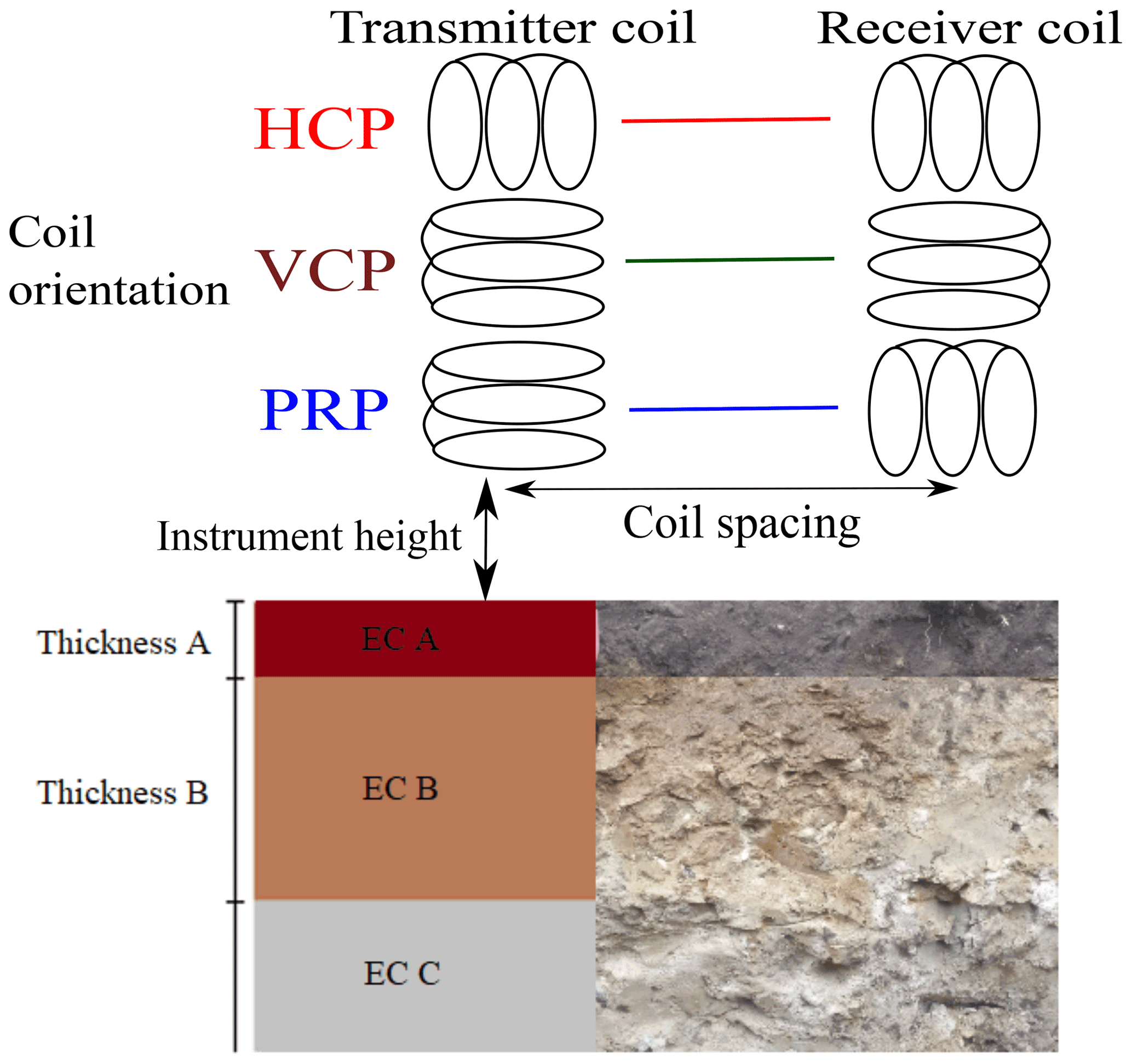
Figure 1 Three-layered soil (A, B, and C layer) with variable electrical conductivities (EC). A schematic of an EMI instrument situated on the surface is also shown. The HCP and VCP have the receiver coil in the same horizontal plane as the transmitter coil. The PRP has the receiver coil in the plane perpendicular to the transmitter coil.

Each of the five soil parameters had 10 possible values, which created 100 000 different EC soil profiles. The ranges of EC used in the forward model were chosen to represent a wide spectrum of soil types and water contents. This is to capture different scenarios of EMI use (e.g., a survey of a large heterogenous area). The lowest EC represents a dry sandy soil, and the highest EC represent an agricultural soil with a combination of high clay or water content (Triantafilis and Lesch, 2005; Robinson et al., 2008; Harvey and Morgan, 2009). The ranges of soil layer thicknesses span from 0.05 to 2.0 m. The full ranges of the subsurface properties are supposed to cover the range of multiple field sites; therefore, we consider a wide range of geology and variation in EC (Palacky, 2011). Each of the three coil orientations was modeled for three different coil separations and three different instrument heights, and the 27 instrument configurations cover both the more typical configurations for field applications of EMI and some more uncommon configurations. In total, the EMagPy code was run 2.7 million times to form the ensemble of results covering the soil and instrument configurations.

Table 1 Adjustable parameters used in the forward model to generate the ensemble and values used for each of the combinations that constitute the soil profiles.

3.2 Analyzing the EMI model results and feature importance with a gradient-boosted decision tree

3.2.1 Decision tree models

Decision tree is a machine learning method that performs regression or classification practicing on subset of the full dataset called training data. A training dataset consists of n samples (x₁,y₁), $(x_{\mathrm{2}},y_{\mathrm{2}}),\mathrm{\dots },(x_n,y_n)$, where x_1−n are the inputs (features), and y_1−n are the corresponding outputs (targets). The aim is to estimate a function F(x) that connects the features with the targets in a way that minimizes the loss function (Friedman, 2001):

$$\begin{array}{}\text{(4)}& L(y,F(x\left)\right)=\sum _{i=\mathrm{1}}^n{\displaystyle \frac{\mathrm{1}}{\mathrm{2}}}[y_i-F(x_i){]}^{\mathrm{2}}.\end{array}$$

The features in our dataset consist of values of modeled EC_a from various instrument configurations, and the targets are the five adjustable subsurface parameters. The tree is built by splitting the values of the features in the training data into two groups. The optimal split minimizes the sum of squared residuals between the value of the targets and the average value of all targets within each group. The two new groups are split into two additional groups each (Hastie et al., 2001). This process continues, creating a structure like an upside-down real-world tree with a root node at the top, from which nonterminal nodes (branches) will occur at every split, and terminal nodes (leaves) at every end point. To avoid overfitting, the growth of the tree is limited by introducing a maximum depth of the tree and a minimum number of data samples required to create a leaf by splitting a nonterminal node.

3.2.2 Gradient boosting algorithm

The gradient boosting (GB) algorithm (Friedman et al., 2001; Mason et al., 1999) takes the training dataset and the chosen loss function to make an initial estimate F₀(x) as a starting point. When the loss function is defined by Eq. (4), the initial estimate F₀(x) becomes the average of the inputs $x_{\mathrm{1}},x_{\mathrm{2}},\mathrm{\dots },x_n$. The residual r_im terms between the initial estimate calculated by F₀(x) and the true value of the targets are calculated for $i=\mathrm{1},\mathrm{2},\mathrm{\dots },n$ as follows:

$$\begin{array}{}\text{(5)}& r_{\text{im}}-{\left[{\displaystyle \frac{\partial L(y_i,F(x_i\left)\right)}{\partial F\left(x_i\right)}}\right]}_{F\left(x\right)=F_{m-\mathrm{1}}\left(x\right)}.\end{array}$$

The right-hand side of the minus sign in Eq. (5) shows the gradient from which the algorithm is named, and the residual r_im terms are named pseudo-residuals. A decision tree model is then made from the features to predict the pseudo-residuals from Eq. (5). The decision tree model output is scaled by a learning rate ν to reduce the variance of the prediction. The scaled output is added to F₀(x) to create a new function F_m(x) for decision tree m for $i=\mathrm{1},\mathrm{2},\mathrm{\dots },n$:

$$\begin{array}{}\text{(6)}& F_m\left(x\right)=F_{m-\mathrm{1}}\left(x\right)+\mathit{\nu }\sum _{j=\mathrm{1}}^{J_m}{\mathit{\gamma }}_{jm}I(x\in R_{jm}),\end{array}$$

where J_m is the total number of leaves in the terminal region R_jm in decision tree model m. The new function F_m(x) is used to calculate a new set of pseudo-residuals. The process of making a new decision tree model F_m(x) and adding the scaled output to the existing function F_m−1(x) is repeated until the reduction in pseudo-residuals with each added tree becomes insignificant or a specified number of trees M has been created.

Feature importance is an indicator of how valuable each of the included features is in the context of the final decision with GB. The relative importance ${\widehat{I}}_j^{\mathrm{2}}$ of any feature is proportional to the number of times it is used to make splits weighted by the square of its improvement to the goodness of fit for the model at each split (Friedman and Meulman, 2003):

$$\begin{array}{}\text{(7)}& {\widehat{I}}_j^{\mathrm{2}}\left(T\right)=\sum _{t=\mathrm{1}}^{J-\mathrm{1}}{\widehat{i}}_t^{\mathrm{2}}\mathrm{1}(v_t=j),\end{array}$$

which sums over the nonterminal nodes J−1 in the tree T and the squared residual ${\widehat{i}}_t^{\mathrm{2}}$ attributed to the split of each node t with v_t as the target variable being split at each node (Friedman, 2001). As boosting generates multiple trees, the relative importance is averaged over all trees. The importance is normalized over all features so that the sum of the feature importance values equals 1, and a higher value indicates a greater effect on the targets.

We found that gradient boosting (Elith et al., 2008; Friedman, 2001) offered improved performance without adding unreasonable additional computational effort, and it was used for all analyses. For our application, each modeled EC_a value in the ensemble of the different EMI configurations represents a feature in ML parlance. We then tested the ability of DT with GB to infer the correct value of each subsurface property given the EC_a that would be measured with all of the EMI configurations. A separate boosted tree was trained to predict each of the five subsurface parameters. The EMI model ensemble was split into training and testing sets using the random sample function in Python: 70 % was used for training, and the remaining 30 % was used for testing. Training and testing were repeated five times with different training and testing splits. Differences among the repeats were small, so all results were combined for analyses. The learning rate, maximum tree depth, and minimum samples per leaf were tuned by manual trial and error, and the optimal values for these parameters were found to be 0.1, 10, and 2, respectively. However, the performance of the DT with GB did not vary significantly with the hyperparameter values. All other hyperparameters used the default values in the scikit-learn toolbox (Pedregosa et al., 2011).

We used the feature importance capabilities of DT with GB to identify which observed EC_a values were most informative for the inference, and we eliminated all insensitive configurations. This allowed us to find the optimal instrument configurations for each subsurface parameter without having to do inverse modeling. To examine the impact of independent knowledge of any of the subsurface properties, we then repeated this analysis for a subset of the soil models that met a given restriction, such as only those that had a thin upper layer or a high-EC middle layer.

3.3 Assessing the value of additional information

For our initial analyses, we considered the full range of all of the subsurface electrical properties. However, in many cases, prior information is available to define one or more of these soil EC parameters or, at least, to reduce the range of plausible values for at least one of them. This prior knowledge could be in form of hard data or soft expert knowledge for a survey area. This study uses layer EC and thickness as prior knowledge, but any information can be considered to constrain the range of cases. Here, we examine how reducing the uncertainty of one soil EC parameter improves the EMI-based inference of other parameter values and whether this additional information changes the composition of the optimal EMI configurations to include in a survey. In addition to the sensitivity of the configurations, this analysis provides the parameter values that result in significantly lowered identifiability of any one of the five subsurface parameters.

To examine the value of additional a priori parameter information, we perform three restriction analyses. In each case, we sequentially limit the range of one of the five subsurface EC parameters and determine the impact on the accuracy of inference of the other parameters. Recognizing that some parameters, especially EC values, can have a different impact on EMI spatial sensitivity if they are too high or low, we consider four patterns of restriction:

• centered – the four minimum and four maximum values defining the parameter ranges are eliminated;

• skewed low – the eight highest values are eliminated from the parameter range;

• skewed high – the eight lowest values are eliminated from the parameter range;

• full range – all 10 possible values of the five parameters are used in the analysis.

For each restriction analysis, we present the impact of the restriction compared with the case with no independent information, and we describe any changes in the composition of the optimal EMI configuration set for each target subsurface parameter.

4 Results and discussion

In this section, we present the outcome from the forward modeling with the full solutions for VCP (Eq. 1), HCP (Eq. 2), and PRP (Eq. 3) as well as the summation from Eq. (4) (Sect. 4.1). We also assess the results from applying a DT with GB to output of the forward modeling. First, we look at parameter identifiability and examine the cases that lead to inaccurate predictions (Sect. 4.2); we then examine the feature importance output (Sect. 4.3). We show the impact of restricting the range of ThickA on inferring ECA (Sect. 4.4.1). Analysis described in Sects. 4.1 to 4.4.1 focuses on the full range of parameters and ECA, the EC of the A layer (the shallowest layer). Finally, we present the impact of the piecewise application of all restriction patterns to all five subsurface parameters on the value of independent information (Sect. 4.4.2) and the feature importance of EMI configurations (Sect. 4.5). The results will be influenced by the choice of forward model, but the ML approach to design optimization is not model dependent and a change in forward model is a trivial extension.

4.1 Modeled EC_a ensemble

The five soil parameters with 10 different values provide us with an ensemble of 100 000 soil profiles. The three coil orientations, three coil spacings, and three instrument heights sum to 27 instrument designs that are applied to each profile. Frequency distributions of the modeled EC_a for each of the 27 instrument designs in all of the profiles are shown in Fig. 2. The distributions are quite similar, but they do differ in detail. The distributions of modeled EC_a values depend strongly on the height or coil orientation for designs with a 1 m coil separation (left column, Fig. 2). The variations are less pronounced for larger coil separations. There are also differences in the smoothness of the distributions: the PRP (bottom row, Fig. 2) has more distinct peaks for small separations, whereas the HCP (top row, Fig. 2) has more peaks for larger separations.

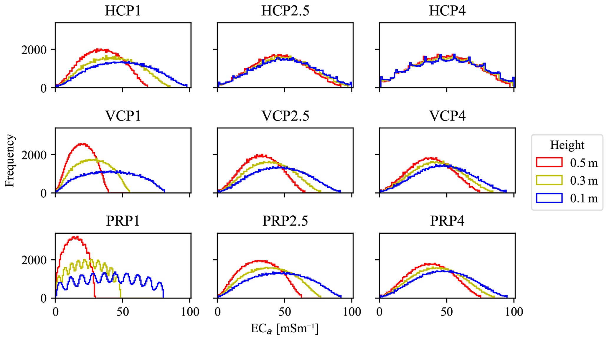
Figure 2 Frequency distributions of the responses from the cumulative sensitivity model for the three coil orientations: horizontal (HCP), vertical (VCP), and perpendicular (PRP). Each panel shows the modeled EC_a output from one coil orientation and coil separation for three different heights. The coil orientation and coil separation change are shown using the respective rows and columns of the nine panels.

4.2 Predicting parameter values with a trained DT with GB using all observations

The first step in our analysis was to examine the ability of the trained DT with GB to predict each parameter value; that is, we used 70 000 EC profile realizations for training the DT with GB. We then provided the 27 observations for each of the remaining 30 000 EC profile realizations to the trained DT with GB and predicted ECA (the EC of the shallowest layer). To account for the brittle nature of DT methods, this procedure was repeated five times with different training and testing splits. The results of the repeated analysis were not significantly different, so they were pooled, providing 150 000 predictions upon which the goodness of fit was determined.

The root-mean-squared error (RMSE) between the predicted and true values of the EC of the A layer (ECA) is shown in Fig. 3. The true values are the known ECA values used in the forward models. The results, shown as a cross-plot of points, are somewhat misleading because it is difficult to see that many points are overlapping close to the 1:1 line. Therefore, shaded areas are included to show ±1 and 2 standard deviations about the mean predicted ECA for each true ECA value. There are clear outliers – cases for which the trained DT with GB did not give an accurate estimate of ECA even considering all 27 EMI observations. However, the overall RMSE was 7.34 mS m⁻¹ over the entire set of 150 000 test cases. The residuals shown in Fig. 3 are not evenly distributed at the low and high values because of the lower and upper boundaries of the input values.

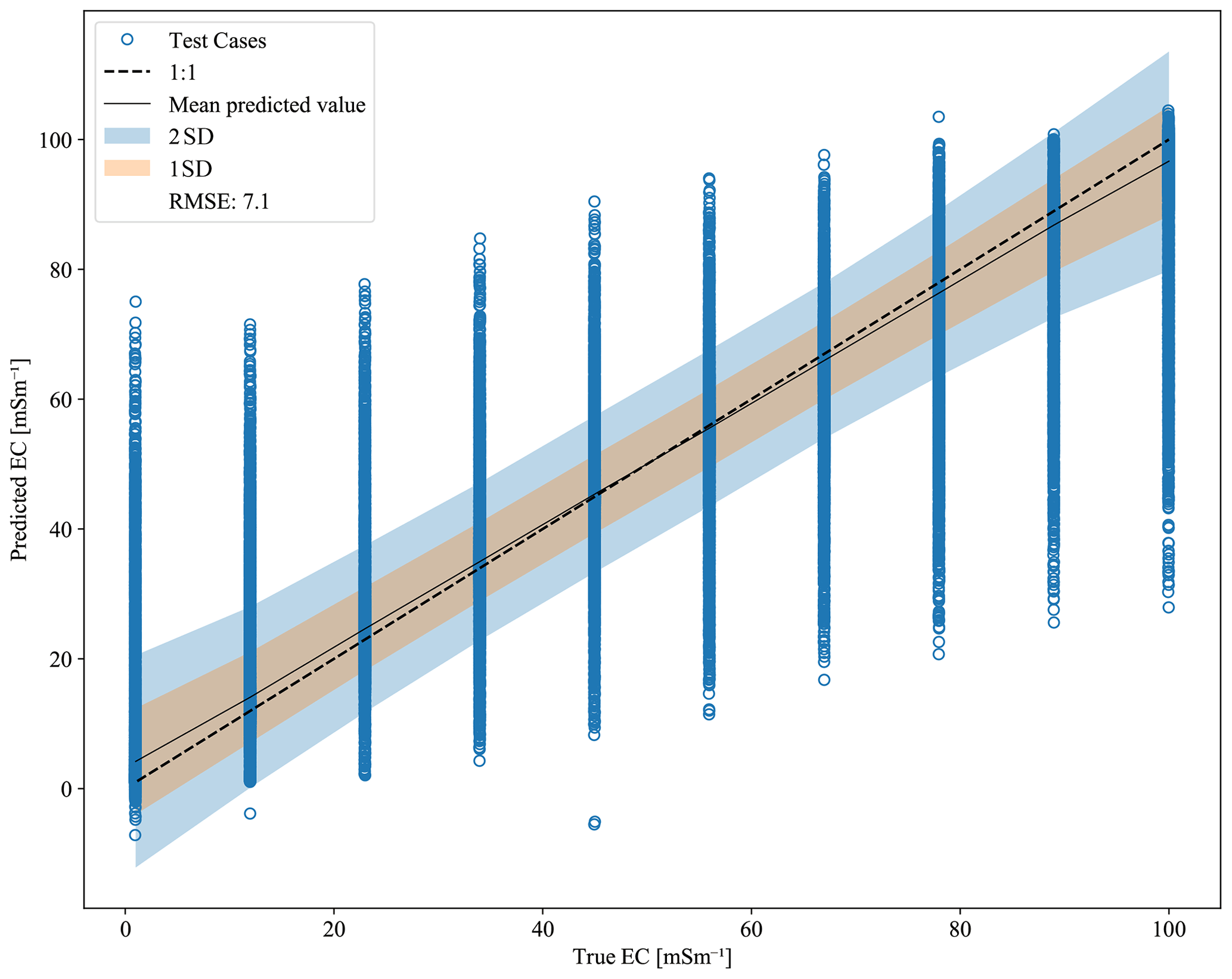
Figure 3 The result of running the DT with GB on the entire 100 000 soil types and all 27 instrument configurations five times. The EC of the A layer (ECA) is the parameter that is being predicted. The x axis is the true value of the ECA, and the y axis is the predicted value of the ECA.

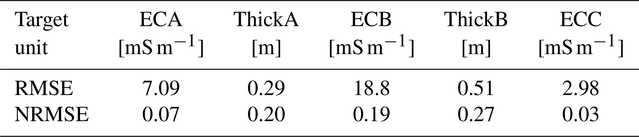
The process shown in Fig. 3 was repeated for each of the five EC profile parameters. The RMSE for each parameter is reported in Table 2, and Table B1 shows how Gaussian noise affects the RMSE. Because the range of values of the parameters differs, the normalized root-mean-square error (NRMSE) is calculated by dividing the RMSE by the full range of the true values of the parameter. The NRMSE of the parameter is a measure of how well the ML can infer the individual parameters and, thus, how estimable the parameters are. As the ML is trained on EMI output, the NRMSE also suggests how well the EMI instrument can detect the soil properties. The results show that EMI is least able to infer the layer thicknesses, with a slightly better ability to infer the thickness of the A layer compared with the B layer. Furthermore, EMI produces better estimates of the shallow and deep EC values compared with the EC of the B layer. These results fit with expectations, given that EMI designs with very short coil separations might be sensitive to only ECA, and those with very large separations might be mostly sensitive to the EC of the deepest layer (ECC) (Callegary et al., 2012; Heil and Schmidhalter, 2015). In contrast, the layer thicknesses, ThickA and ThickB, and the EC of the middle layer (ECB) must always be inferred based on multiple measurements.

Table 2 The root-mean-square error (RMSE) between the prediction from the gradient-boosted (GB) model and the testing data. The machine learning procedure was repeated with each of the five subsurface parameters as targets, thereby creating five models. The RMSE is normalized by the mean value of the target to get the normalized root-mean-square error (NRMSE).

4.2.1 Examining the conditions that led to poor estimations of ECA

From the 150 000 test cases displayed in Fig. 3, 8816 cases are more than 1 standard deviation away from the true value when predicting ECA. These cases are displayed using the blue markers that are located outside the shaded areas (Fig. 3). The compositions of these 8894 cases are presented as frequency distributions of their parameter values in Fig. 4. The values for ECB, ECC, and ThickB are uniformly distributed, which indicates that no specific values of ECB, ECC, or ThickB lead to poor inference of ECA. In contrast, 94 % of the problematic conditions have a thickness of the A layer (ThickA) among the three lowest values. This, again, agrees with expectations that the EC of a thin layer would be more difficult to infer accurately than that of a thicker layer using an EMI instrument. The opposite is found for ECA; while not as pronounced, the results indicate that the poorly inferred cases tended to have higher ECA values, with 54 % of the conditions having the three highest ECA values. This suggests that identifying the layer with an EMI instrument would be more likely to be successful if the range of ThickA did not include the lowest values examined here; that is, we would expect improved inference of ECA for restrictions of ThickA that are centered or skewed high. A more successful survey, based on the ability to infer ECA, would occur if the ECA values tend to be lower; that is, a restriction that is centered or skewed low should show better performance.

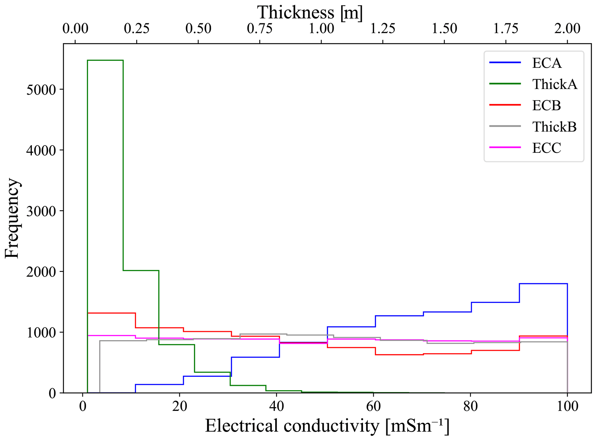
Figure 4 The ECA was inferred for 150 000 test cases. In 8816 of the 150 000 cases, the inference was more than 1 standard deviation away from the true value. The figure shows the distribution of five subsurface parameter values within the 8894 conditions. The top x axis is the layer thickness, the bottom x axis is the layer EC, and the y axis is the frequency.

4.3 Feature importance when predicting parameter values with a trained DT with GB

The preceding analysis used measurements from all 27 instrument configurations for each EC profile parameter estimation. The major focus of this investigation was to use ML tools to identify the optimal set of observations to collect, which balances performance with reduced field effort. To illustrate how the built-in feature importance of tree-based methods can be used to achieve this, consider the results shown in Fig. 5. The feature importance is shown for each of the 27 configurations; because they sum to 1, it is convenient to represent this as a pie chart. The colors and patterns that comprise the circles identify the eight most important EMI configurations for each combination of the parameters. The fraction of the circle covered by each color and pattern shows the relative importance of that observation. The colors indicate the coil orientation, while the shade and pattern indicate the coil distance and instrument height. The 19 least important EMI configurations are combined in “others” (white slices). From these results, it is apparent that approximately 90 % of the information used to predict ECC (rightmost circle) is provided by configuration HCP_4.0_0.1. The optimal orientation and large coil separation could have been predicted from McNeil's classic work (McNeill, 1980). However, the aforementioned study did not consider the PRP orientations. The reason for the preference for a small instrument height is apparent: it may simply be due to further penetration of the signal to greater depth. To our knowledge, no other method, short of exhaustive comparisons of many synthetic inverse analyses, would have been able to show that a single configuration, among the full suite of instruments, was so clearly dominant for inferring ECC. Similarly, almost 60 % of the information used to infer ECA (leftmost circle) was provided by the PRP_1.0_0.1 configuration. The small coil separation and low instrument height fit with general expectations, and the highly sensitive PRP orientation fits with the findings of Tabbagh (1986).

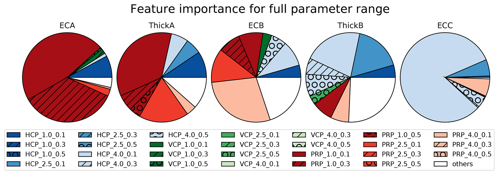
Figure 5 Feature importance for inferring each of the five parameters from a decision tree analysis of the full parameter range. The feature importance of all 27 configurations sums to 1. The eight most important configurations for inferring each of the five parameters are shown using a unique color and pattern combination. The remaining 19 configurations are aggregated into the “others” category and displayed in white.

Taken together, the results suggest that each of the EC profile parameters relies on a relatively small number of observations. To illustrate this, 90 % of the importance, including only the most important observations, is provided by 4, 9, 13, 17, and 3 observations for ECA, ThickA, ECB, ThickB, and ECC, respectively (Fig. 5). Of these highly important observations, 53 % had the instrument placed at the lowest instrument height considered. The VCP is the most widely used coil orientation in agriculture (Heil and Schmidhalter, 2017), but it is only 17 % of the most informative configurations use the VCP orientation (Fig. 5). This may be explained by the spatial sensitivity of the orientations (Callegary et al., 2007; Christiansen et al., 2016) which indicates that the HCP and PRP pairing is more complementary relative to the HCP and VCP pairing. The influence of simulated noise on the results in Fig. 5 is shown in Appendix B.

4.4 Parameter restriction analyses

4.4.1 Applying a restriction to the thickness of layer A that is skewed low

One piece of information that may be available (e.g., from direct field examination) is the expected thickness of the shallow topsoil layer (ThickA). Therefore, we begin our restriction analyses by examining the effect of improved knowledge of ThickA on the inference of the ECA parameter. Specifically, we repeated the analysis only including models with the two middle values of ThickA (0.69 and 0.86 m). This reduces the ThickA parameter range to 11 % of its full range and, therefore, removes the cases that contain low values for ThickA. The results (Fig. 6) show stark improvement in the ability of the DT with GB to infer ECA. A similar analysis could be repeated for any restricted range of values for any parameter or for multiple parameters. This could be done for practical reasons – to design a site-specific survey – or for scientific reasons – to explore which conditions are identifiable with EMI and to understand these parameter interactions.

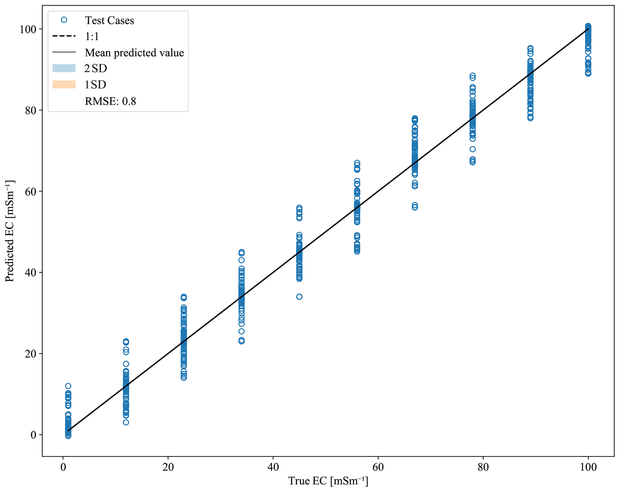
Figure 6 The result of running the machine learning algorithm on a subset of the ensemble where the thickness of the A layer has been restricted. Only 20 000 soil types and all 27 instrument configurations remain in this restricted subset. The EC of the A layer (ECA) is the parameter that is being predicted.

The analysis leading to Fig. 6 is one example of the ability of the DT with GB method to consider the benefits of independent soil property information. In this section, we expand the investigation to include all of the soil electrical parameters and three different restriction patterns.

4.4.2 Changes in the parameter inference of restricted subsets

Figure 7 summarizes the impacts of providing the maximum amount of additional information (considering only 2 of the 10 possible values of one parameter) on the inference of all other parameters. The y axis of Fig. 7 is the RMSE (such as that reported in Fig. 6 for inferring ECA with ThickA restricted) normalized by the full range (maximum–minimum) of the inferred parameter. With reference to Fig. 6, this would be reported as the RMSE divided by the range of ECA, giving a unitless value of 0.028. Each inferred parameter is associated with a short horizontal line, which indicates the normalized RMSE without restriction of any other parameter's range. Each symbol in Fig. 7 represents the results of an analysis like that shown in Fig. 6. There are three symbols (triangle, dot, and square) associated with each target and restricted parameter pair for each of the three restriction patterns. Consider, for example, inferring ECA. The set of three blue symbols represents the impact of restricting the range of ECA itself: the leftmost triangle represents a restriction that is skewed low (retaining the two lowest ECA values), the middle dot is a centered restriction (ECA values 45 and 56 mS m⁻¹), and the right square represents a restriction that is skewed high (retaining the two highest ECA values). As expected, restricting the range of ECA, regardless of the restriction pattern, leads to a similar reduction in the normalized RMSE of ECA. Every pair of restricted and inferred parameters is represented using three symbols with the same left-nudged triangle, center dot, and right-nudged square for restrictions that are skewed low, restrictions that are centered, and restrictions that are skewed high, respectively.

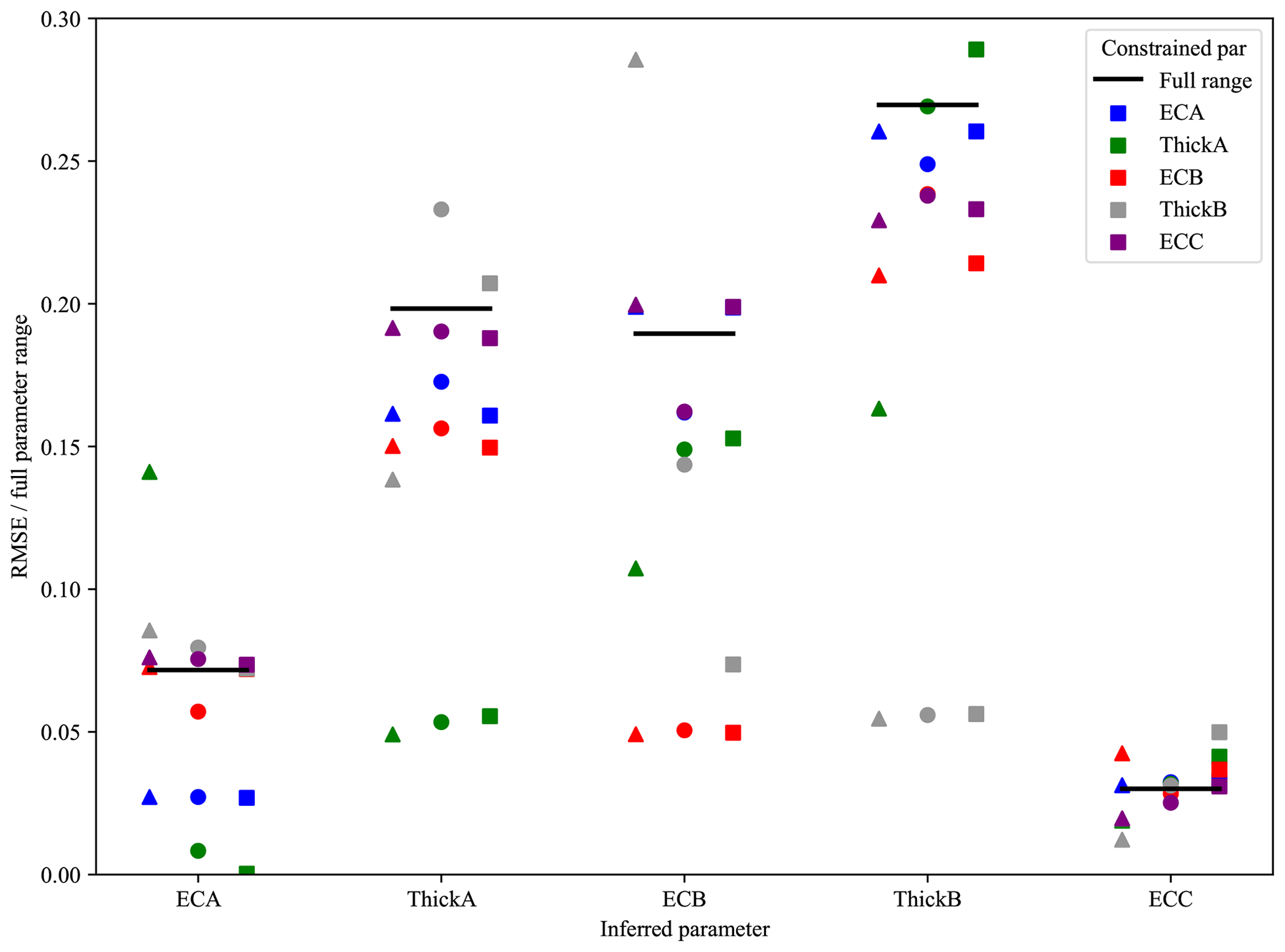
Figure 7 The changes in the inference of the five subsurface parameters (x axis) are based on a comparison between the RMSE from the restricted case divided by the range of the parameter (y axis). The lines show how well the parameters are predicted when all parameters are full range. The color shows the parameter that is being represented, and the location and symbol represent the three restriction patterns: skewed low (left-nudged triangle), centered (centered dot), and skewed high (right-nudged square).

Consider another example to illustrate how Fig. 7 can be interpreted and related to Fig. 6. The three symbols' dots above ECA represent the impact of restricting ThickA. The center dot corresponds exactly to Fig. 6, the centered restriction of ThickA. The left green triangle shows that there is an increase in the NRMSE for the restriction that is skewed left compared with the unrestricted case (horizontal line above ECA), which shows that restricting the thickness of layer A to the lowest range of values leads to lower-quality inference of ECA. In other words, the shallowest layer may be too thin to be detected properly because the instrument response is an integration over a large depth compared with the now relatively thin layer thickness. This fits with previous findings (Fig. 4), which revealed that a thin ThickA makes it difficult to infer ECA. Furthermore, it agrees with our expectations that if the uppermost layer is sufficiently thick, we can choose a coil separation and orientation that is almost exclusively sensitive to the uppermost layer, essentially allowing direct measurement of ECA. Consistent with this explanation, the right green square above ECA has the lowest NRMSE. In this case, this confirms the expectation that it is easier to infer ECA accurately if the shallowest soil layer is relatively thick. Similar interpretations about the value of restricting one parameter on the ability to infer other parameters accurately can be drawn for each pair of restricted and inferred parameters, allowing researchers to gain valuable insight into the interaction of measurements and other independent information. In all cases, there is a reduction in the NRMSE of the inferred parameter when the parameter itself is restricted. For these cases, there are no significant differences among the three restriction patterns. In most cases, restricting the range of the inferred parameter itself showed a greater improvement than restricting any other parameter. The only clear exception was inferring ECA, which showed a greater improvement by restricting ThickA with a central or right skew.

Consider the inferred parameter ThickB in Fig. 7. The three green symbols represent the cases where ThickA is restricted. The left triangle is the restriction that is skewed low and results in a reduced NRMSE compared with the full parameter range (black line). The middle dot, which is the centered restriction, shows the same NRMSE as the full parameter range. The right square, which is the restriction that is skewed high, has a higher NRMSE than the full parameter range. The changes in NRMSE between the three restrictions of ThickA show that knowledge of the ThickA confers little advantage to estimating ThickB unless it can be shown that the shallowest layer is very thin.

More generally, there are relatively few cases where the restriction of one parameter significantly improves the inference of another parameter. Beneficial restrictions include restricting ECA and ECB to infer ThickA and restricting ThickA and ECA to infer ECB. To a lesser degree, restricting any other parameter when inferring ThickB offers a slight advantage. The value of ECC is already well constrained for the full parameter range, as shown by the line, and there is little advantage to restricting another parameter to infer ECC. In 37 % of cases, restricting the range of one parameter led to worse inference of another. These cases display the field conditions that lead to more challenging use of EMI, such as a very thin middle layer making it very difficult to infer ECB. An experienced EMI user would be able to reach these conclusions, which helps us to confirm that the ML approach is robust and reaches reasonable results. The value of this type of analysis with a geophysical EMI model is to provide guidance for site-specific conditions, but the analysis can also be executed with more complete geophysical models or different model types. Furthermore, this guidance is quantifiable rather than based on intuition derived from the rule of thumb.

4.5 Feature importance in restricted subsets

The composition of the optimal EMI measurement configuration is different depending on the soil layer thicknesses and conductivities. Figure 8 summarizes the feature importance for the cases presented in Fig. 7, for which only 2 out of 10 values remain for the restricted parameter. The color and symbol patterns are the same as those used for Fig. 5. The columns in Fig. 8 represent the five inferred parameters, and the rows represent the restricted parameter. Consequently, each circle is a pairing between one restricted and one inferred parameter. The circles are subdivided into four rings that represent the different restriction patterns. From inside out, the rings represent the full parameter range (no parameter restriction), a centered restriction, a restriction that is skewed low, and a restriction that is skewed high. The feature importance of the full parameter range (centermost ring) is the same in every row for each inferred parameter. For reference, the center ring results are identical to those presented in Fig. 5. All 75 combinations of the five inferred and restricted parameters and the unrestricted case are shown for the three restriction patterns in Fig. 8, allowing a user to draw general insights into the value of different configurations under a wide range of conditions. Figure 8 is designed to showcase all of the different combinations' restrictions made to the ensemble in this study; however, for pure practical application, not all combinations would need to be displayed.

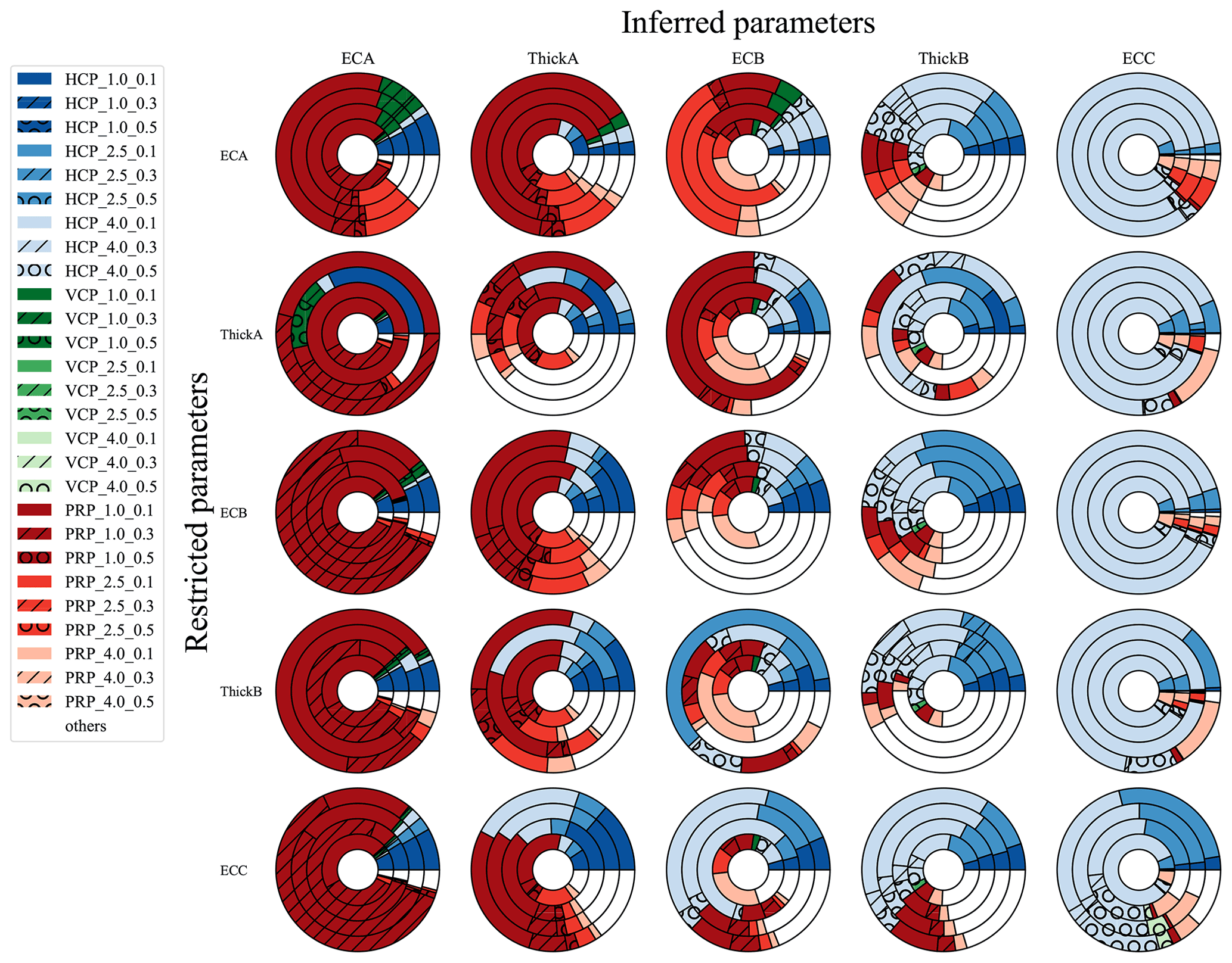
Figure 8 Feature importance for the eight most important EMI configurations for every combination of the five inferred and restricted parameters and the three patterns. Each circle is subdivided into four rings that show, from inside out, the feature importance for the full range, a centered restriction, a restriction that is skewed low, and a restriction that is skewed high. Each column (row) represents each of the five inferred (restricted) parameters. The coil orientations are colored so that horizontal (HCP) is blue, vertical (VCP) is green, and perpendicular (PRP) is red. Dark and light hues represent a short and long coil distance, respectively.

Figure 8 is somewhat information dense, so it may be useful to discuss a few cases in more detail. One of the simplest subplots to understand is the inference of ECC when restricting ECA (top right circle). The results show clearly that there is no meaningful change in the composition of the optimal set of configurations due to adding additional ECA information, regardless of the range of ECC values considered: all four concentric rings look nearly identical. Furthermore, all four rings indicate that a single configuration, HCP_4_0.1, provides the vast majority of the information needed to characterize ECC. Again, this is in general agreement with the rules of thumb derived from the 70 % rule, but it confirms these findings for all values of EC and thickness of the other layers, and it extends the findings to consider the PRP configuration. Moving down the ECC column, note the difference when ThickB is restricted. If ThickB is skewed high (ThickB ranges between 1.8 and 2.0 m), there is some advantage to adding the PRP_4_0.1 configuration. Our approach does not explain this choice. We suggest that it is informative to collect this additional observation to constrain the values of ECB and ThickB if the middle layer is relatively thick and that the identified configuration has a usefully different sensitivity distribution than the large HCP array placed close to the ground surface. This result could not be anticipated based on the rule of thumb. Furthermore, the resulting optimal configuration is almost identical if either ThickA or ThickB is restricted, when inferring ECC. Moving to the bottom of that column, the analyses show that if the value of ECC itself is limited, the composition of the optimal set changes significantly. Interestingly, regardless of the pattern of restriction (the results are almost the same for the outer three rings), the optimal set now includes four configurations with approximately equal importance: HCP_4_0.1, HCP_4_0.5, HCP_2.5_0.1, and PRP_4_0.1. It is further confirmation of the validity of the approach that no VCP arrays were chosen, as would be expected based on McNeil (1980). Similarly, as expected, the larger array separations are preferred. It is surprising, however, that one of the four observations place the instrument higher above ground. This is a result of the spatial sensitivity and an example of a conclusion that is very difficult to reach through intuition and the rule of thumb. This could point researchers to ask follow-on questions about why a specific configuration or observation type are identified as optimal.

The results for inferring ECA (leftmost column) are similar but show interesting differences. The optimal set for ECA is relatively insensitive to the pattern of restriction of ECA; however, more than one observation is required for all cases. While the optimal cases were similar for restricting ThickA and ThickB for inferring ECC, this similarity holds for restricting ECB and ThickB when inferring ECA. The pattern of restriction of ThickA has dramatic impacts on the optimal set of configurations for inferring ECA. Inferring the three other parameters (ThickA, ThickB, and ECB) shows significant changes in the optimal configuration set depending upon the pattern of restriction (ring to ring) and upon the independent information provided (row to row). There is no case for which a single configuration dominates the importance in all rows. In fact, there are many cases that would recommend more than nine configurations. For example, this likely indicates that ThickB is unlikely to be well resolved by a practical field survey. Further considerations of inferring ThickB give interesting general insights compared with rule-of-thumb suggestions. Namely, very few VCP configurations are selected. If PRP arrays are to be used, profiling should be achieved using multiple coil separation pairs with the coil placed close to the ground. For HCP configurations, profiling should be achieved by increasing the coil separation.

To summarize, taken together, Figs. 7 and 8 provide guidance to an EMI user when designing a survey with a specific target. Figure 7 indicates whether that target can be characterized reliably given the full range of configurations considered and which additional information will improve the characterization. A low NRMSE will suggest a more reliable characterization of the subsurface property by the instrument and vice versa. Figure 8 identifies the optimal set (and number) of arrays needed for optimal characterization. Some of the conclusions would be expected based on the simplified descriptions from the classic work of McNeil (1980) and would be anticipated by an experienced EMI user. Other results would be difficult, if not impossible, to predict without a “value of data” analysis like that shown here. These results, in particular, could point the way to further scientific investigations to better understand the complementary information content of multiple EMI configurations. The restriction analyses offer insight into the mutual identifiability of soil EC. Given the availability and flexibility of EMagPy (McLachlan et al., 2020) and the efficiency of the DT with GB algorithm, the analyses performed here could be extended to include the identification of optimal configuration sets for multiple targets (e.g., thickness and EC of the B layer). For example, placing equal weight on all five targets, an optimal without restriction of any of their values suggests the use of one HCP array (HCP_4.0_0.1) and four PRP arrays (PRP_1.0_0.1, PRP_4.0_0.1, PRP_1.0_0.3, and PRP_2.5_0.1). If this specific set of configurations was deemed impractical, a user could limit the available configurations for consideration, find the optimal survey, and compare the projected RMSE to that estimated for the overall optimal set. This information could guide a user on whether it is worthwhile changing their instruments (or designs) or whether gathering additional information about the range of plausible parameter values is likely to be more important for their survey goals.

In this study, 27 instrument configurations in combination with 100 000 subsurface models are considered the full ensemble. Using the presented ML approach to assess the data value for our full ensemble is more efficient than an inverse (Furman et al., 2007; Khodja et al., 2010; Song et al., 2016) or sensitivity (Hanssens et al., 2019) approach. In some cases, evaluating all instrument configurations will not be necessary, which means that the inverse or sensitivity approaches become more efficient. The ML approach requires a certain size of model ensemble to yield stable results; therefore, the model run time will reduce efficiency. However, this affects the inverse analysis more because it generally requires more model runs. Ultimately the efficiency of the ML, inverse, and sensitivity approaches depends, in the EMI case, on the model run time, the number of layers, the parameter boundaries, and the number of considered configuration, and the combination of these in the applied case will determine which method is more efficient. Designing a combination of optimal configurations based on a conceptual understanding of the spatial sensitivities (rule of thumb) is not a reasonable task. Furthermore, measurement optimization requires a quantitative measure of the information content. The ML approach provides a quantitative measure of the shared information among model parameters (Table 2 and Fig. 7) to compare the likely success of each configuration.

Finally, the general approach shown here could be extended easily to consider multiple measurement types (e.g., combining EMI with other geophysical methods) and even the dynamic optimization of measurement networks for monitoring applications.

5 Conclusions

Most environmental and agricultural field investigations are conducted on relatively limited budgets. As a result, there is usually some advantage to optimizing data collection to achieve the best results with the limited time and money available. These restrictions are one of the main reasons that electromagnetic induction (EMI) has become a popular tool for these studies. While it is often the case that the measurements are more ambiguous than direct measurements of soil properties, the noncontact nature of the instruments allows for much greater spatial coverage. The recent availability of EMagPy (McLachlan et al., 2020) allowed us to perform the large number of EMI forward models necessary to support a machine learning (ML) examination of EMI surveys, leading to a simple but comprehensive investigation of parameter identifiability and optimal EMI configurations. The result is an approach that can allow an EMI user with limited expertise to choose a better set of instrument configurations given their main survey goal and knowledge of the site conditions. The same tool can point more advanced users to areas of investigation that may improve our understanding of the prior knowledge content of different EMI configurations. The decision tree with gradient method based on a large ensemble of instrument response forward models (proposed here) makes novel use of the efficiency and built-in feature importance capabilities. However, the analyses are not restricted to this relatively simple ML algorithm. More advanced ML tools could be combined with independent feature importance analyses, if required, for specific monitoring applications. Similarly, while EMI forward modeling is relatively simple and fast, given that it is based on analytical models, with sufficient computational resources any measurement method and underlying physical process could be examined in the same way. As just one illustrative example, an optimal combination of EMI, electrical resistivity, gravity, and monitoring well observations could be proposed to constrain the interpretation of a pumping test performed in an unconfined, anisotropic medium by conducting forward models of many configurations (survey locations and times, electrical resistivity tomography array types, and screen depths) for a large ensemble of plausible aquifer conditions and allowing an ML algorithm to consider all of the data and identify the most informative observations. This opens the possibilities for exploring truly novel combinations of multimodal observations.

Appendix A: Symbols and abbreviations

CS	Cumulative sensitivity
DT	Decision trees
EC	Electrical conductivity
ECa	Apparent electrical conductivity
ECA, B, and C	Electrical conductivity of layers A, B,
	and C, respectively
EMI	Electromagnetic induction method
GB	Gradient boosting
HCP	Horizontal coplanar
LIN	Low induction number
ML	Machine learning
NRMSE	Normalized root-mean-square error
PRP	Perpendicular planar
RMSE	Root-mean-square error
ThickA and B	Thickness of layers A and B, respectively
VCP	Vertical coplanar

Appendix B: The effect of noise on inferring subsurface parameters and feature importance

To assess the impact of noise, 100 realizations of heteroscedastic Gaussian noise with a standard deviation of 0.05 were carried out. The ensemble from the full solution was multiplied by the random noise prior to ML application to the full ensemble (no restrictions). This was repeated for each realization of noise, and the average fit and their standard deviation are shown in Table B1.

The average feature importance over the 100 realizations (Fig. B1) affects ThickA, ECB, and ThickB the most. Here, the feature importance is distributed more evenly among the configurations compared with without noise.

Table B1 The root-mean-square error (RMSE) between the prediction from the gradient-boosted (GB) model and the testing data. The machine learning procedure was repeated with each of the five subsurface parameters as targets, creating five models.

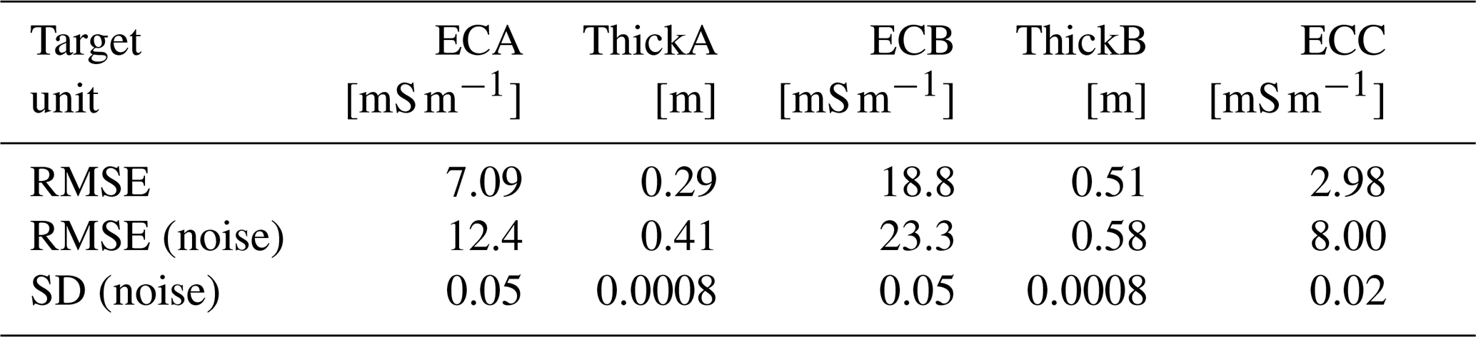
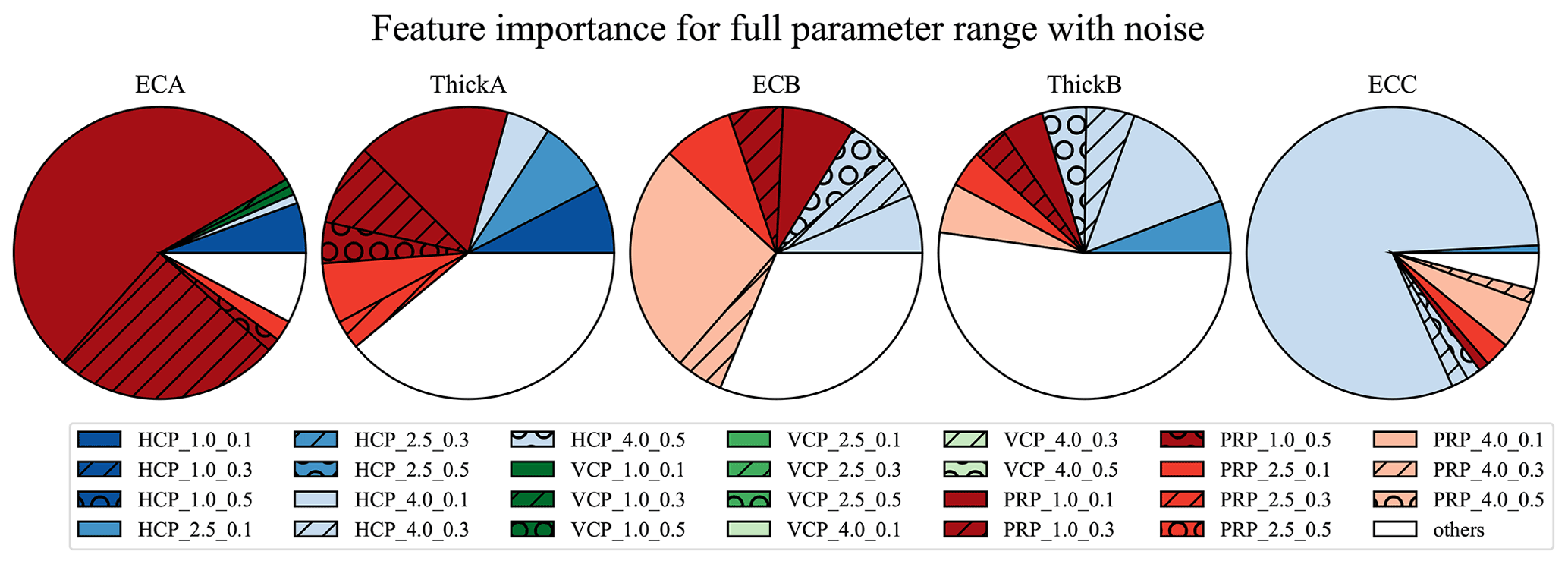
Figure B1 Feature importance for inferring each of the five parameters from a decision tree analysis of the full parameter range. The feature importance of all 27 configurations sums to 1. The eight most important configurations for inferring each of the five parameters are shown using a unique color and pattern combination. The remaining 19 configurations are aggregated into the “others” category and displayed in white.