the Creative Commons Attribution 4.0 License.
the Creative Commons Attribution 4.0 License.
 | 27 Oct 2022
Pitfalls and a feasible solution for using KGE as an informal likelihood function in MCMC methods: DREAM(ZS) as an example
Yan Liu
Jaime Fernández-Ortega
Matías Mudarra
Andreas Hartmann
The Kling–Gupta efficiency (KGE) is a widely used performance measure because of its advantages in orthogonally considering bias, correlation and variability. However, in most Markov chain Monte Carlo (MCMC) algorithms, error-based formal likelihood functions are commonly applied. Due to its statistically informal characteristics, using the original KGE in MCMC methods leads to problems in posterior density ratios due to negative KGE values and high proposal acceptance rates resulting in less identifiable parameters. In this study we propose adapting the original KGE using a gamma distribution to solve these problems and to apply KGE as an informal likelihood function in the DiffeRential Evolution Adaptive Metropolis DREAM(ZS), which is an advanced MCMC algorithm. We compare our results with the formal likelihood function to show whether our approach is robust and plausible to explore posterior distributions of model parameters and to reproduce the system behaviors. For that we use three case studies that contain different uncertainties and different types of observational data. Our results show that model parameters cannot be identified and the uncertainty of discharge simulations is large when directly using the original KGE. The adapted KGE finds similar posterior distributions of model parameters derived from the formal likelihood function. Even though the acceptance rate of the adapted KGE is lower than the formal likelihood function for some systems, the convergence rate (efficiency) is similar between the formal and the adapted KGE approaches for the calibration of real hydrological systems showing generally acceptable performances. We also show that both the adapted KGE and the formal likelihood function provide low performances for low flows, while the adapted KGE has a balanced performance for both low and high flows. Furthermore, the adapted KGE shows a generally better performance for calibrations of solute concentrations. Thus, our study provides a feasible way to use KGE as an informal likelihood in the MCMC algorithm and provides possibilities to combine multiple data for better and more realistic model calibrations.
- Article
(8246 KB) - Full-text XML
-
Supplement
(813 KB) - BibTeX
- EndNote


Markov chain Monte Carlo (MCMC) techniques are extremely useful in uncertainty assessments and parameter estimations of hydrological models (Smith and Marshall, 2008). Among those MCMC methods, Vrugt et al. (2008, 2009) developed a DiffeRential Evolution Adaptive Metropolis (DREAM) algorithm, which has found numerous applications in various fields (Vrugt, 2016). It is an adaptation of the SCEM-UA algorithm (Vrugt et al., 2003a) that can efficiently estimate the posterior probability distribution of model parameters in the presence of high-dimensional and complex response surfaces with multiple local optima.
The formal likelihood function, e.g., mean square error (MSE) or root mean square error (RMSE), obtained from first-order statistical principles based on error series derived from simulations and observations, is commonly used in the DREAM algorithm. The formal likelihood function strongly relies on error assumptions, which can highly influence the shape of parameter posterior distributions (Beven et al., 2008). The informal likelihood functions, such as Nash-Sutcliffe efficiency (NSE) and the alternative Kling–Gupta efficiency (KGE) are often used in hydrological studies to indicate the general performance of model simulations (Gupta et al., 2009). These metrics represent an important measure of model performance, so-called goodness of fit (Pool et al., 2018). These likelihood functions are not directly derived from stochastic error series, but can be easily used to combine different types of data.
There are studies that discussed how to adjust the calculation of NSE in order to overcome the problems using NSE in MCMC methods. For example, McMillan and Clark (2009) introduced a constant K into the adapted NSE calculation. By adjusting this constant, they can mimic the weight such that small improvements in NSE can also be distinctly identified leading to the chain evolution. They even found that the informal likelihoods can provide a more complete exploration of the behavioral regions of the response space and hence more accurate estimation of total uncertainty (McMillan and Clark, 2009). Freer et al. (1996) introduced a parameter as an exponent symbolled with N. They argued that higher N values have the effect of accentuating the weight given to the better simulations.
However, how to properly use KGE in the MCMC methods has not been studied. Directly using KGE in MCMC methods, e.g., the DREAM algorithm, may raise difficulties such as incorrect posterior ratios due to negative KGE values, and nonlinearity between model performance and KGE values. These difficulties essentially affect chain evolutions such as the acceptance rate, indicating how easy a proposal is accepted, and the convergence rate, denoting how fast a chain converges to a stationary distribution. As a consequence, considering the computational cost with a limited number of realizations in practice, the informal character of KGE and its use in MCMC methods influences the exploration of posterior parameter distribution and model uncertainty, such as the density of identifiable parameters. Studies showed that using informal likelihood functions in generalized likelihood uncertainty estimations (GLUE) may lead to unsatisfactory posterior distributions of model parameters (Mantovan and Todini, 2006; Stedinger et al., 2008). Using NSE as the likelihood function, the number of measurements cannot be considered. Therefore, with increasing numbers of measurements the information added to the performance measure is little, thus preventing the improvement of chain evolution (Mantovan and Todini, 2006). Therefore, to feasibly use KGE in MCMC methods requires solving problems in drawing better proposals to avoid a very flat posterior distribution, to account for the influence of observational size (the amount of information included in calibration) on parameter estimations and to achieve reasonable acceptance and convergence rates.
In this study we propose adapting the gamma distribution and KGE to find a feasible solution for properly using KGE as an informal likelihood function in DREAM(ZS). We test the robustness of this approach with three case studies representing known and unknown systems with varying numbers of observations and also different types of data using two hydrological models (a lumped and a semi-distributed). The aim of our study is to attempt to form the probability calculation based on KGE in a pseudo formal way. The derivation of probability based on KGE in a statistically sound manner is beyond the scope of this study and will need future work. We compare the performance between the original KGE, GLUE (generalized likelihood uncertainty estimation), the formal likelihood function, the log-transformation and the adapted KGE. We aim to show whether the adapted KGE is robust and plausible to explore posterior distributions of model parameters and to reproduce the hydrological behaviors. Thus, we will compare performance (1) regarding acceptance, convergence, and uncertainty between the adapted KGE, the original KGE, a formal likelihood function and a log-transformation, (2) regarding discharge simulations in terms of general performance, variability, bias and correlation for total, low and high flows and (3) model performance combining discharge and solutes. These comparisons allow us to provide recommendations for more reliable applications of KGE in MCMC methods in different research areas.
2.1 Kling–Gupta efficiency
Kling–Gupta efficiency (KGE) takes account of variability (α), non-scaled bias (β) and correlation (r) by computing the Euclidian distance (ED) of the three components from the ideal point, which avoids the underestimation of variability and enables the comparison of the bias term between catchments (Gupta et al., 2009).
with and , where (μs, σs) and (μo, σo) are the mean and standard deviation of simulations and observations, respectively. KGE ranges from −∞ to 1 with the optimal value at unity. A value larger than −0.41 indicates that a model improves on using the mean (Knoben et al., 2019).
2.2 Adapting KGE in DREAM(ZS)
2.2.1 Basics of DREAM(ZS)
DREAM(ZS) is one type of DREAM algorithm, which uses sampling from an archive of past states to generate candidate points in each individual chain. It automatically tunes the scale and orientation of the proposal distribution towards the target distribution and maintains a detailed balance and ergodicity (Vrugt et al., 2008, 2009). We take DREAM(ZS) as an example and investigate the appropriate way to use KGE within DREAM(ZS). As our goal is to adapt KGE as an informal likelihood function, we focus on the Metropolis probability, , which calculates the probability to accept a proposal.
where and p(Xi) denote the probability density of the proposal and the present location of the ith chain, respectively. If is larger than a random value drawn from the uniform distribution U(0, 1), the proposal will be accepted, otherwise the chain remains in the present location. After chain evolutions, the Gelman-Rubin convergence diagnostic is computed for each parameter j={1, …, d}. If , the convergence can be declared.
where N and T signify the number of chains and the number of samples in each chain, respectively, Wj is the within-chain variance, and is an estimate of the variance of the jth parameter of the target distribution.
We choose the easily applied formal likelihood function (lik = 11 in Table B1, Vrugt, 2016) to calculate the log-likelihood (LogL), which assumes the error residuals to be normally distributed. It is described as
where et(X) denotes the tth error residuals and n is the total number of observations.
2.2.2 Deriving pseudo probability density based on KGE
Based on abovementioned basics of DREAM(ZS), using KGE as a likelihood function becomes the question of obtaining the proper calculation of pseudo probability density . From the straightforward and easily applied way, one would directly use KGE as by setting the negative KGE values to zero. However, it results in two problems (Fig. 1):
-
Problem 1: the probability density needs to be positive in order to get a positive ratio to determine the right orientation to accept a proposal. However, KGE ranges from −∞ to 1. Setting negative KGE values to zero can work, but then we lose the orientation of proposals with negative KGE values. Thus, it reduces the efficiency of chain evolution.
-
Problem 2: the model performance does not linearly increase with the linear increase of KGE. Therefore, directly using positive KGE as the pseudo probability density will lead to a high possibility to accept poor proposals. For instance, the probability is 0.75 () to accept a proposal with KGE = 0.6 under the present sample with KGE = 0.8. However, the performance of a simulation with KGE = 0.8 is much better compared to that with KGE = 0.6.
We propose solving these two problems by adapting the gamma distribution and KGE to derive a proper probability density (Fig. 1). The gamma distribution has two parameters, the shape parameter (k) and the scale parameter (θ), and is evaluated for variables with positive values. When the shape parameter k=1, the probability distribution is one-sided with non-linear decreasing probability for increasing variable values. Therefore, we can use 1 − KGE (ranges from 0 to ∞) as the variable for gamma distribution and get higher probabilities for larger KGE values. When choosing the scale parameter θ=0.5, the increasing rate of probability becomes faster when KGE > 0.5 and especially when KGE > 0.7 the probability increases much faster. This helps chain evolution to find proposals which lead to high model performance. The non-linear increase of probability with increasing KGE is shown as the red line in the top right box of Fig. 1. The log-likelihood is used in DREAM(ZS), thus we derive the pseudo log-likelihood (LogL) using gamma distribution and KGE. To include the influence of observation size on the parameter estimations, analogous to the formal likelihood function, we take account of the number of observations (the term in the formal log-likelihood) in deriving the pseudo log-likelihood. Finally, we have the pseudo log-likelihood using KGE and gamma distribution as
where, f( ) is the γ probability density function, k and θ are the shape and scale parameters, respectively, n is the number of observations and X represents the parameter vector of the calibrated model. The purpose of this approach is to provide a feasible way to incorporate KGE as the informal likelihood function for MCMC methods, in our case DREAM(ZS). Another goal is to achieve similar performance as when using the formal likelihood function such as RMSE so that we can compare the model simulations and predictions between formal and informal (our approach, KGE) likelihood functions.

Figure 1Concept of adapting KGE in DREAM(ZS). It shows the problems of using the original KGE as the likelihood function in DREAM(ZS) and how to adapt gamma distribution and KGE to get a proper informal likelihood.
2.3 Case studies
To test the robustness of our new approach, we define three case studies: (1) true and pseudo-analytical posterior distributions of model parameters are known by a virtual experiment, and uncertainties in model structures and input data are absent, (2) calibrations and evaluations with a long observation time series using a rainfall-runoff model, which allows comparing the performance between three approaches by varying the amount of data in calibration. The parameterization of the system is unknown and there are uncertainties in model structure, input data and observations and (3) a model calibration combining hydrodynamics and simple solute transport for a more complex karst system with a large subsurface heterogeneity and processes for fast recharge and groundwater discharge from conduit networks. The observation period is short and uncertainties exist in model structure, input and observation data, and model parameter estimations.
2.3.1 Case study 1: virtual experiment
We generate a virtual experiment using a rainfall-runoff model (the HBV model). We obtain the forcing data, daily mean temperature and daily precipitation (2001–2008), from the German site in Liu et al. (2021). The HBV model represents typical catchment rainfall-runoff processes considering one soil water storage and two groundwater storages (Lindström et al., 1997). In this virtual experiment, we use the model version without snow processes, which contains nine parameters. As our goal is not the model itself but the calibration of model parameters, we only provide descriptions of model parameters (Table 1). For the model structure and equations, refer to Liu et al. (2021).
Table 1Names, description, ranges and virtual true values of the HBV model parameters for the virtual experiment.
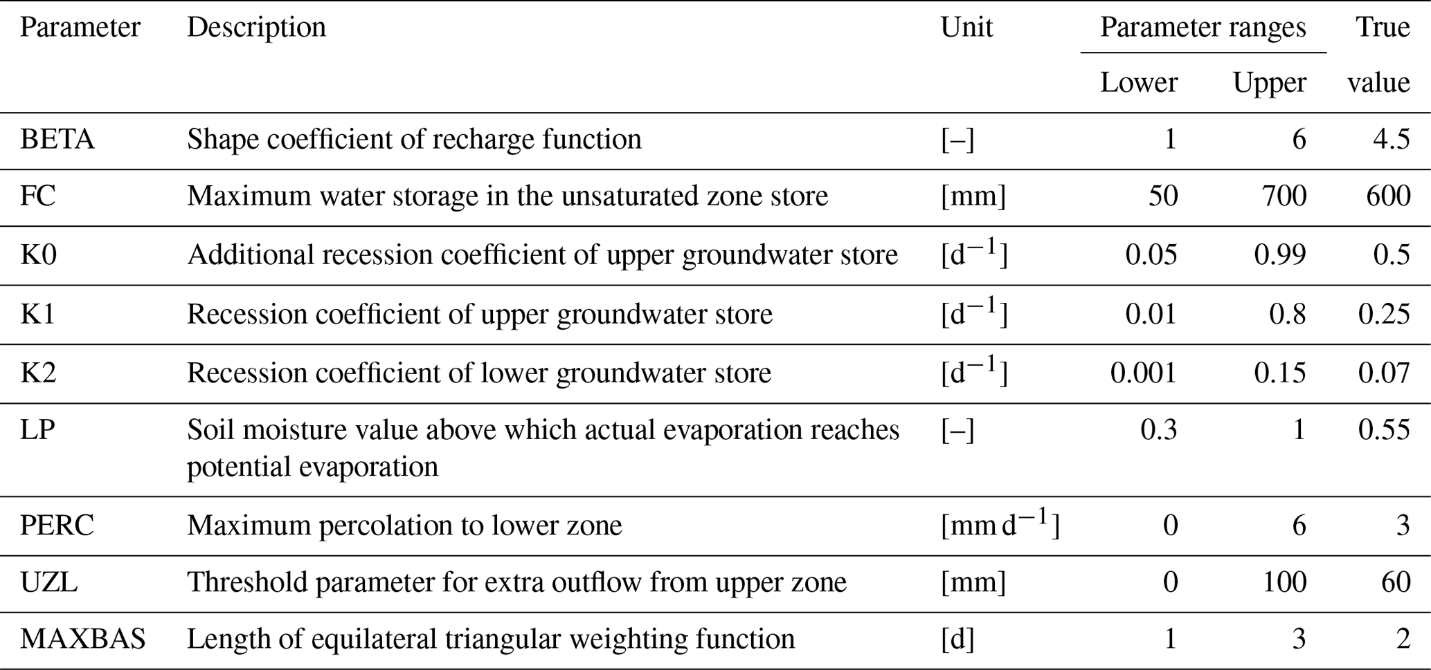
Note: K0, UZL and MAXBAS are insensitive parameters in this case study and thus are fixed to the true values.
As the analytical posterior distributions of model parameters of a hydrological model are hardly achievable, we use the following procedure to generate the pseudo-analytical posterior distribution. Firstly, we set the catchment area of 100 km2 and run the model with “true” parameters for 2004–2008 to obtain the simulated discharge. Secondly, assuming a normal distribution for error residuals (a common assumption for hydrological modeling), we generate random values from a normal distribution (mean = 0, standard deviation = 5 % of the mean simulated discharge) and add these random values as measurement errors to the simulated discharge to form the observations. Finally, due to no uncertainty in input data and model structure, using this setting for measurement errors we can use the formal likelihood function (Eq. 5) to derive the pseudo-analytical posterior distribution of model parameters. We performed a local parameter sensitivity analysis before model calibrations to find insensitive parameters (K0, UZL and MAXBAS in Table 1, changing these parameters only affects model performance KGE by 0.001). Therefore, we fixed the three parameters in calibration, resulting in six parameters to be calibrated.
2.3.2 Case study 2: long observations for rainfall-runoff modeling
In order to test the capability of our approach for a real system with uncertainties in forcing, observations, model structure and model parameters, we select a catchment from the CAMELS-US dataset (Newman et al., 2014, 2015) and simulate the rainfall-runoff processes with the HBV model as case study 1. We also compare the performance of our transformed KGE with the GLUE method. We have the following criteria to select this catchment: (1) catchment area is between 100 and 500 km2 to avoid the influence of channel routing, (2) the snow fraction is zero to avoid the snow processes to reduce the HBV model parameters and the number of parameters remains nine (Table 1) and (3) the carbonate rock fraction is zero as we will test a karst catchment as a separate case study. We then choose the first catchment (smallest number in catchment ID) that fulfills our criteria, the catchment 02246000 (gauging station at North Fork Black Creek near Middleburg, FL, USA), shown in Fig. 2. It has a catchment area of 451 km2 with the mean annual precipitation of 1352 mm. The main land cover is savanna, accounting for 77 % of the total area. Details of the catchment properties can be found in CAMELS-US dataset (Newman et al., 2014, 2015).
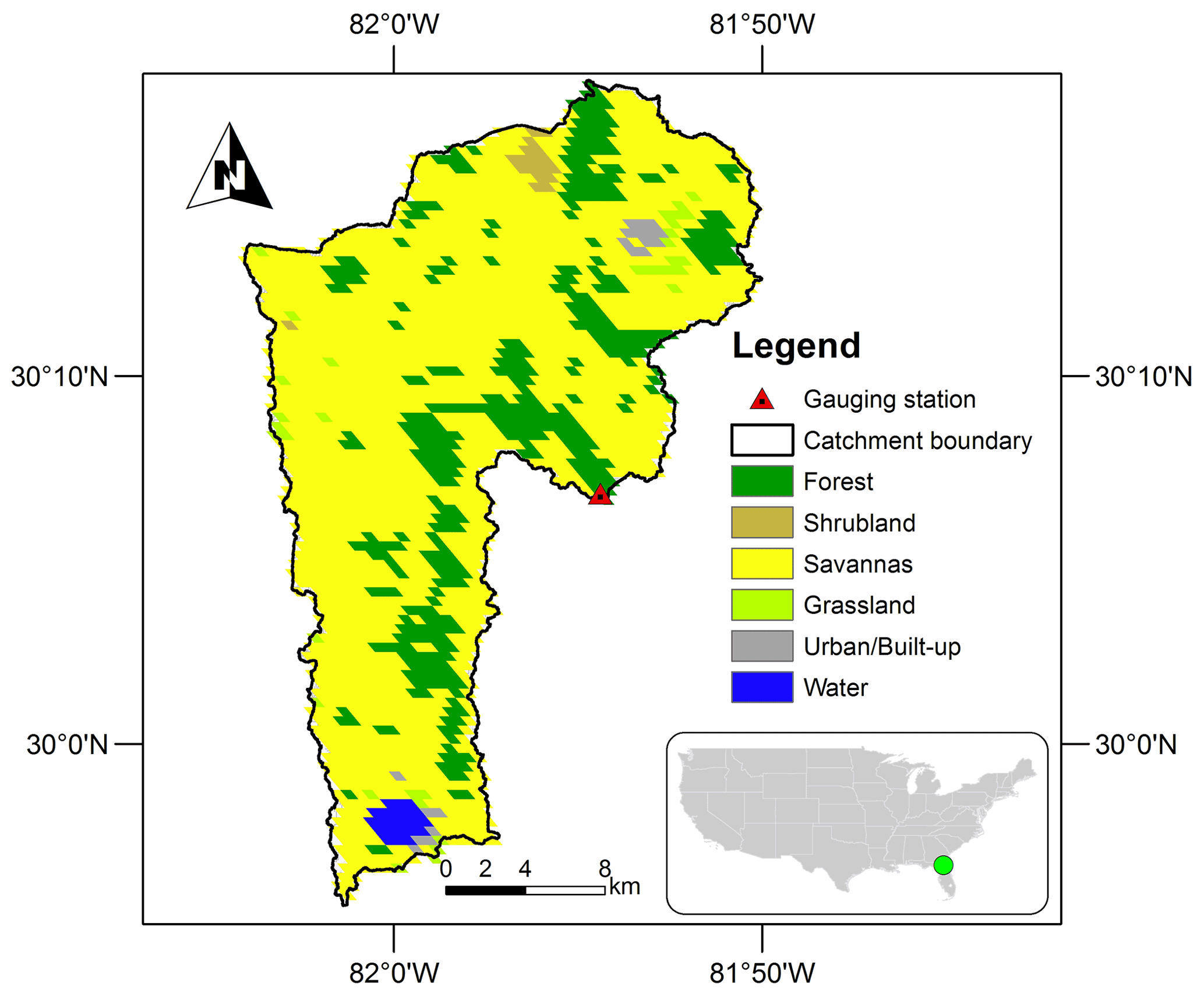
Figure 2Study area of the catchment with the gauging station at North Fork Black Creek near Middleburg, FL, USA for the case study 2.
2.3.3 Case study 3: short observations for a heterogeneous karst system
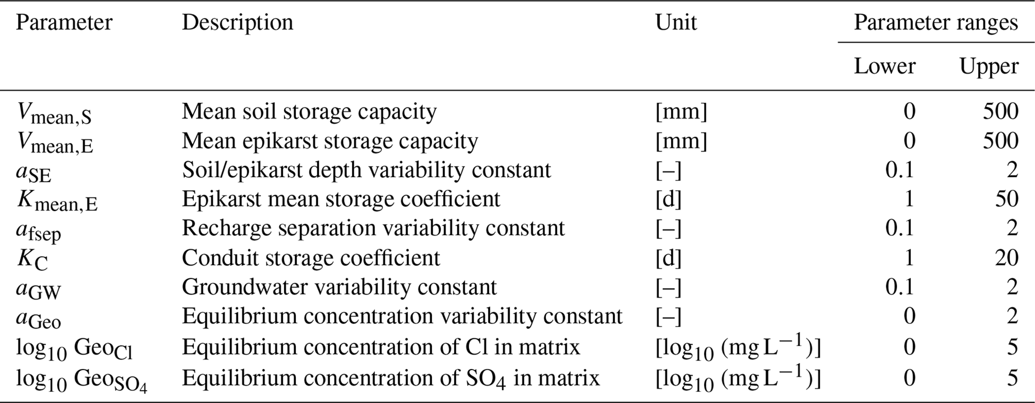
In order to test the capability of our new approach for a complex system, we set case study 3 in a karst system that has conduit systems resulting in fast recharge and discharge. It has uncertainties from the forcing data, the model structure and observation errors. Daily discharge time series and weekly solute (Cl−, and ) concentrations of the hydrological years 1 October 2006–30 September 2009 are combined for model calibrations. The study site (Fig. 3) is located in southern Spain with a recharge area of 13.85 km2 (the study site in Hartmann et al., 2014). In this case, we use the same model, the VarKarst model with the solute transport routine, for spring discharge and solute simulations as it was successfully applied to this site before (Hartmann et al., 2014). The VarKarst model is a semi-distributed hydrological model, which considers subsurface heterogeneity, soil and epikarst storage dynamics and groundwater hydrodynamics. It uses a mixing routine to simply reproduce the solute transport. These processes are represented by 10 parameters (Table 2). Details of the VarKarst model processes and assumptions can be found in Hartmann et al. (2014). Discussion of the transport processes is beyond the scope of this study, we therefore choose the same processes as published in Hartmann et al. (2014). Our study then focuses on comparing the performance of different calibration approaches.
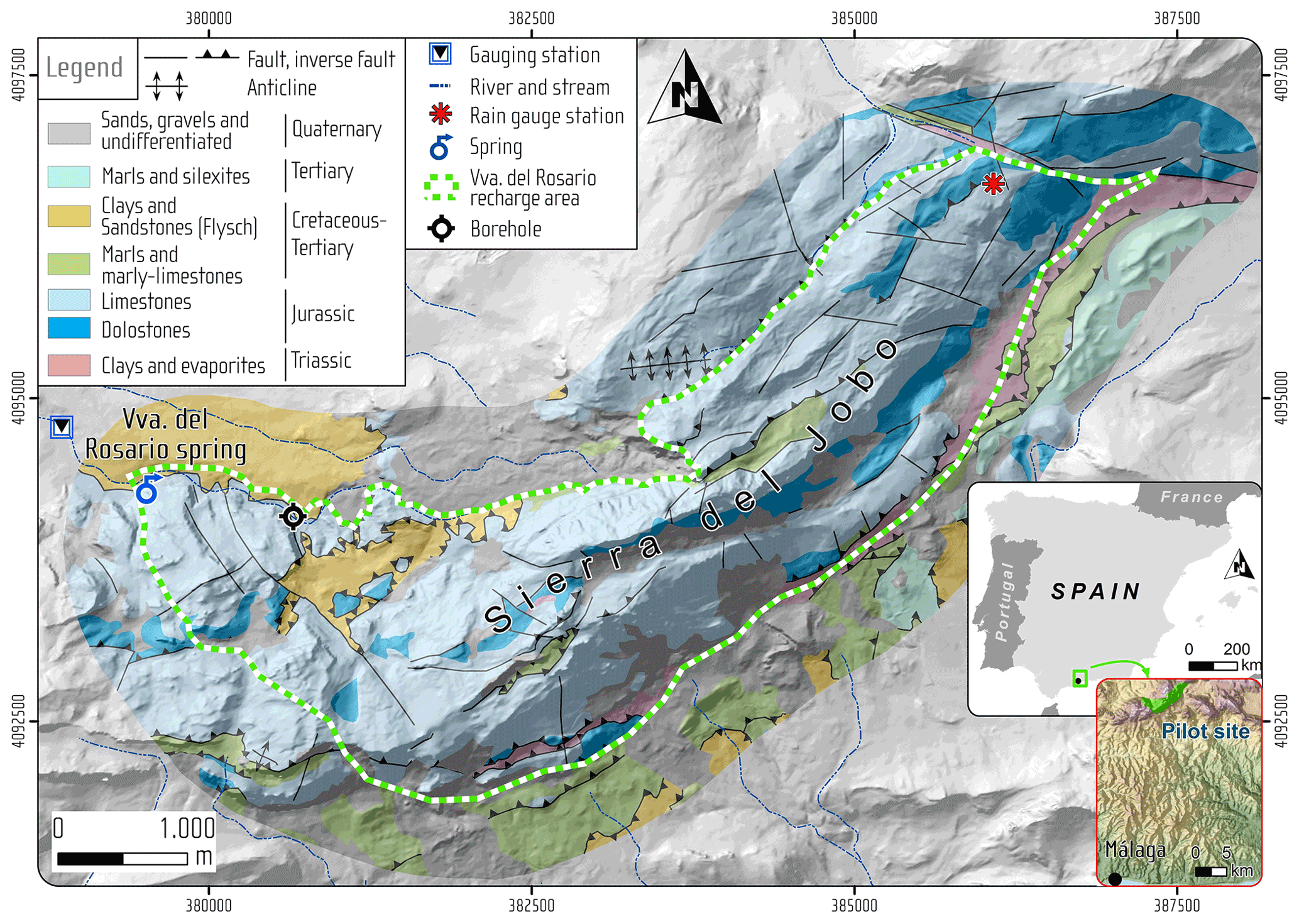
Figure 3Study area of the Rosario Spring for case study 3. This map is an updated version of the map in Hartmann et al. (2014).
Table 2Names, descriptions and ranges of the VarKarst model parameters.
2.3.4 Calibration and evaluation
For calibration of the three case studies, we have used the GLUE approach and DREAM(ZS) with different likelihood functions: (1) using the original KGE as the likelihood function (“KGEori” thereafter), here negative KGE is set to zero to avoid negative posterior density ratios, (2) using the traditional formal likelihood assuming error is normally distributed (“formal” thereafter), (3) using the log-transformation (“formallog” thereafter), which is suggested as being good for low flows (McInerney et al., 2017) and (4) using our new approach adapting gamma distribution and KGE to derive the pseudo log-likelihood (“KGEgamma” thereafter). We use three parallel Markov chains (default setting in DREAM(ZS)), and set 20 000 realizations for case studies 1 and 2, but 30 000 realizations for case study 3 (due to more processes and parameters). The last 25 % of the realizations are used to approximate the posterior distributions and the corresponding parameter sets are used for the discharge simulations in the evaluation period. They are also used to derive the parameter uncertainty and the total simulation uncertainty (parameter uncertainty + randomly sampled error from a normal distribution with mean = 0 and standard deviation = RMSE of the simulation with the maximum a posteriori parameter) in DREAM(ZS).
For case study 1, following a standard calibration procedure we use 2001–2003 as the warm-up period and 2004–2008 as the calibration period. The posterior distribution of model parameters derived from DREAM(ZS) using the formal likelihood function is deemed as the pseudo-analytical posterior distribution. By comparing to it, we can investigate whether calibrations using KGEori and KGEgamma can explore the right posterior distribution and true model parameters.
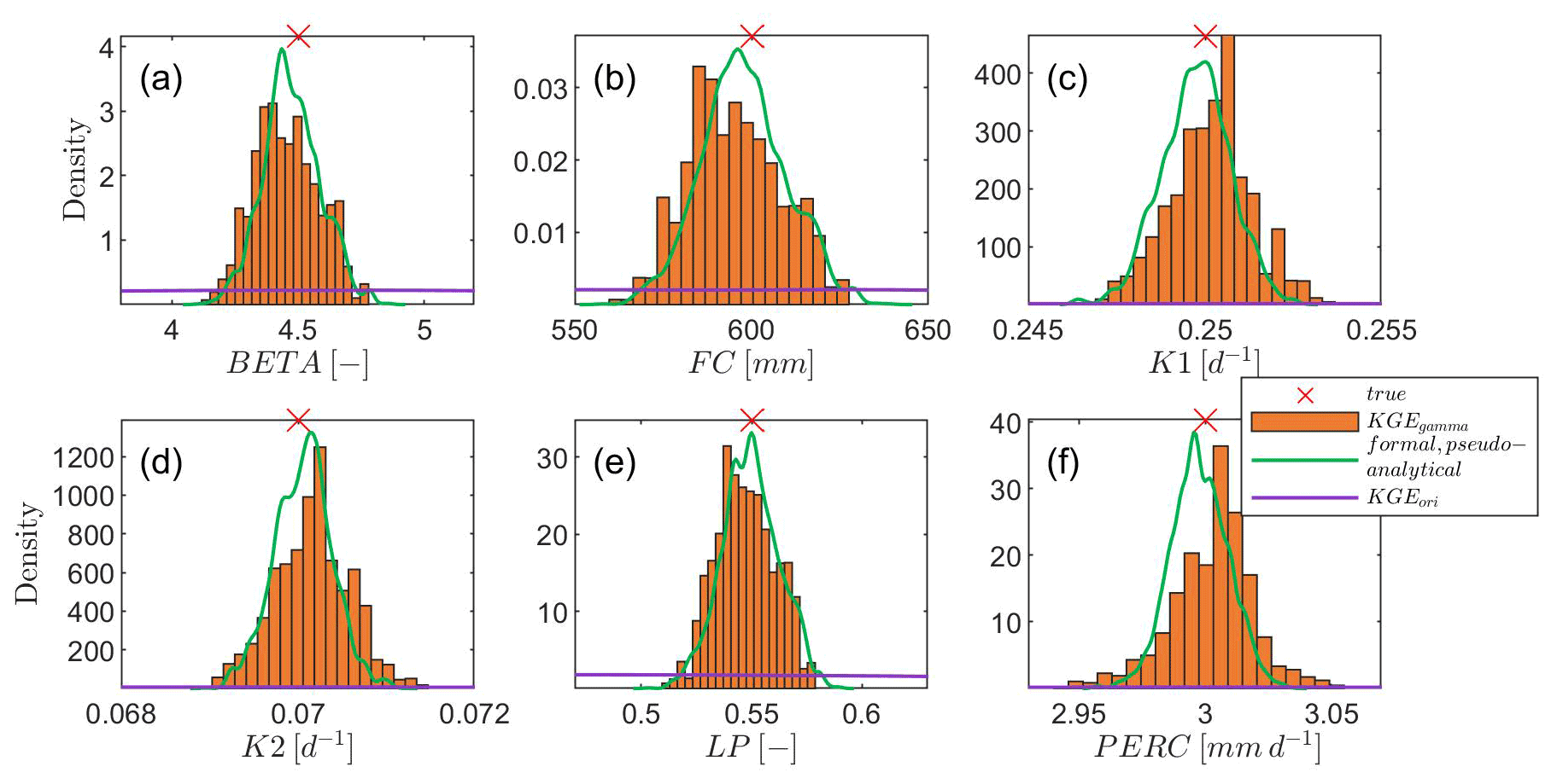
Figure 4Posterior distributions of sensitive model parameters for the virtual experiment. The red cross symbol denotes the true model parameter value. KGEori indicates using the original KGE (set negative KGE to zero) as the likelihood function, while KGEgamma represents our new approach using gamma distribution and KGE to derive the probability density, and the case formal, pseudo-analytical means pseudo-analytical posterior distribution derived from the formal likelihood function. Note that the density of using KGEori is very low and close to the x axis.
For case study 2, the true model parameters are unknown. We use 25 hydrological years (1 October 1980–30 September 2005) to perform the calibration and evaluation. We choose the Daymet forcing data to drive our hydrological model as these meteorological data have potential evapotranspiration (PET) estimates and were used to calculate the catchment climatic properties (Addor et al., 2017). We use the first 5 years as the warm-up period, then the following 10 years for calibration and the last 10 years for evaluation. We test the performance of 4 approaches (GLUE, formal, formallog and KGEgamma) using 1, 3, 5, 8 and 10 years of observations for calibrations to check the capability of the 4 approaches for calibration of a real system with varying amounts of available observations. For the GLUE method, we use the Nash-Schetcliff efficiency (NSE) as the objective function. We set 20 000 realizations and choose the top 25 % in performance (kept the same as DREAM(ZS)) as the behavioral parameter sets to explore the posterior distribution.
For case study 3, the true model parameters are unknown too. We calibrate the hydrodynamics and solute transport simultaneously. For calibrations using the formal likelihood function, we normalize each observation variable by its mean to exclude the influence of units and magnitudes of discharge and solute concentrations. We compare the performance of three approaches: (i) we use the formal likelihood function and use the normalized daily discharge and normalized weekly concentrations of three solutes as the combined observations (“formalnorm” thereafter). Here we do not consider the difference in the total number of observations between discharge and three solutes (the total number of discharge observations is 10 times the number of each solute), (ii) we also use the formal likelihood function but we replicate each normalized solute observations 10 times to have the same weight for discharge and each solute (“formalnorm,w”). Issues regarding different weights for discharge and solutes and different ways to obtain weights are out of the scope of our study and (iii) we use the KGEgamma approach. Firstly, we calculate KGE for discharge and each solute using their observations and simulations (a total of four KGE values for discharge, Cl−, and ). Then we calculate the mean of the four KGE values (equal weight for the four variables, same as ii) and use it in the KGEgamma approach. We use 3 hydrological years (1 October 2003–30 September 2006) for warm-up of the simulations and the 3 following hydrological years (1 October 2006–30 September 2009) for calibration. This is the same as the calibration setting in Hartmann et al. (2014) considering the short observations of each solute.
The model performance for calibration and evaluation is examined using KGE and its three components representing variability (α), bias (β) and correlation (r). The calculations of KGE, α, β and r refer to Eqs. (1) and (2). We evaluate the model performance using the four metrics for total flow, low flow (smaller than the 10th percentile of observed discharge) and high flow (larger than the 90th percentile of observed discharge) and also for three solutes.
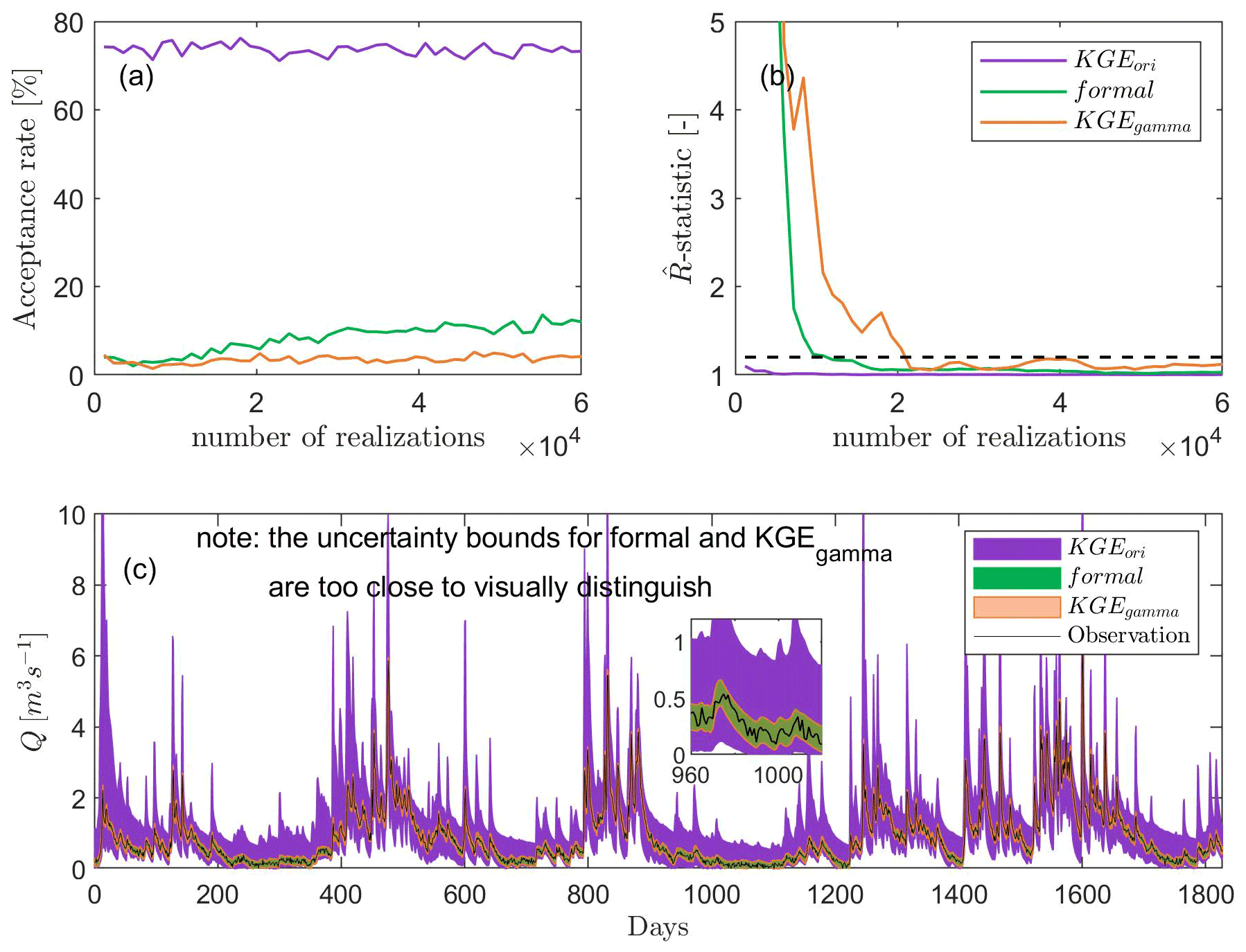
Figure 5Acceptance rate (a), convergence rate shown with -statistic (b), and uncertainty of discharge simulations (total uncertainty) for the virtual experiment (c). KGEori indicates using the original KGE as the likelihood function, while KGEgamma represents our new approach using gamma distribution and KGE to derive the probability density, and the case formal means using the traditional formal likelihood function. Note the uncertainty bounds for formal and KGEgamma are too small to be visually seen.
3.1 Case study 1: posterior parameter exploration
When using the original KGE (set negative KGE values to zero) as the likelihood function, the posterior parameter range is only slightly reduced for all sensitive parameters compared to the prior uniform distribution. In addition, the density around the true values of model parameters is still very flat, indicating that true model parameters are barely identified (Fig. 4). When applying the adapted KGE (adapting the gamma distribution and KGE to derive probability density), the posterior parameter range is much more reduced and the reduced range is more or less centered at the true values as shown in Fig. 4. Compared to the pseudo-analytical posterior distributions of all model parameters derived from the formal likelihood function using the special virtual setting, the adapted KGE approach (KGEgamma) shows similar magnitude and shape regarding the posterior distributions. It suggests that our adapted KGE approach performs similarly to using the traditional formal likelihood function and can explore the right parameter posterior distributions.
As expected, using the original KGE we have a very high acceptance rate (ca. 60 %–80 %, Fig. 5a), leading to a very fast convergence (Fig. 5b). This results in a large uncertainty bound in the discharge simulations (Fig. 5c), and the uncertainty of peak discharges is particularly large. With the adapted KGE, we see that the acceptance rate becomes smaller and the convergence gets slower. This can be explained by introducing the nonlinearity of the adapted KGE: probability densities for large and small KGE values are more distinct compared to the original KGE. Figure 5a also shows that the acceptance rate of our approach is 5 %–10 %, which is lower than ca. 20 % of the formal likelihood function. Similarly, the convergence rate of our approach is slower than the formal likelihood function (Fig. 5b). This suggests that using the formal likelihood function has a higher efficiency than the approach adapting KGE for calibrations of a system that only contains little uncertainty (only small observation errors in our case). However, when more uncertainties appear, e.g., uncertainties in forcing data and model structures, the convergence rates (efficiency) become similar between the adapted KGE and the formal likelihood function (refer to the following subsections, Fig. 6b). Compared to the width of the discharge uncertainty bound using the original KGE (Fig. 5c), calibration using the formal likelihood function and the adapted KGE both reduce the average width of total discharge uncertainty bound by ca 85 %. As this virtual experiment does not assume uncertainty in the input data and the model structure, the adapted KGE shows a similar performance in the uncertainty estimation to using the formal likelihood function and both can closely reproduce observations.
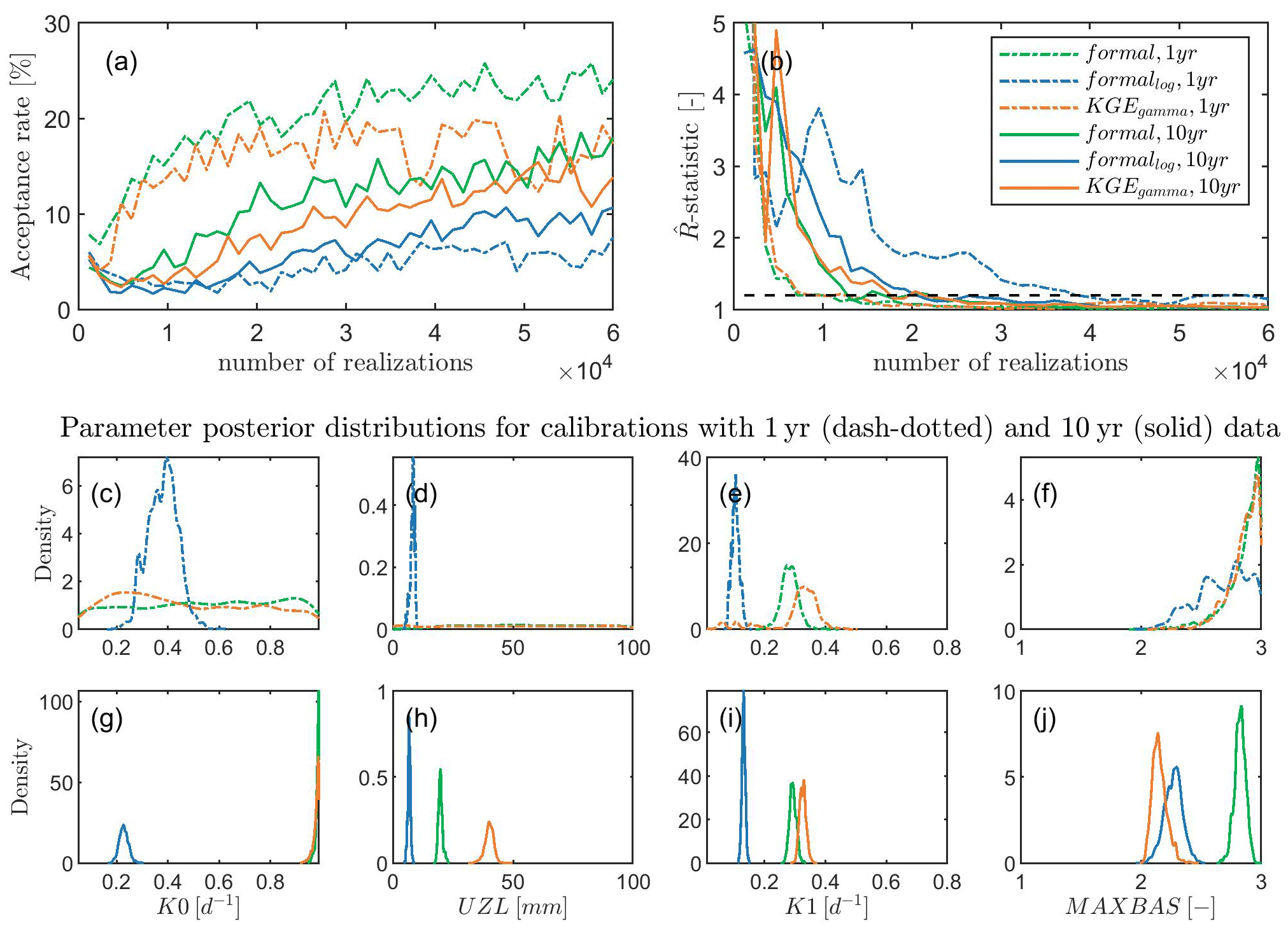
Figure 6Acceptance rate (a), convergence rate shown with -statistic (b), and posterior distributions of selected parameters for calibrations with 1-year (c–f) and 10-year (g–j) observations, respectively. KGEgamma represents our new approach using gamma distribution and KGE to derive the probability density, the case formal means using the traditional formal likelihood function, and formallog means using the log transformation. The subscripts 1 yr and 10 yr denote calibrations with 1-year and 10-year observations, respectively. The four parameters (nine parameters in total) are selected to represent different cases from unidentified (less observations for calibrations) to identified (more observations for calibrations) parameters and show how the identified parameters change when using different amounts of observations for calibrations.
3.2 Case study 2: model parameter calibrations with long observations
For calibrating a real system (with uncertainties in forcing, observations, and model structure and parameters), the acceptance rate of the adapted KGE is lower than that of the formal likelihood function, but higher than that of the log-transformation (Fig. 6a) for calibrations using both short and long observations. The convergence rate is almost identical between the formal likelihood function and the adapted KGE (higher than the log-transformation, Fig. 6b). This indicates that our approach has a same efficiency as the formal likelihood function and a higher efficiency than the log-transformation for calibrations of a system with more uncertainties. With more observations in calibrations, the unidentified parameters K0 and UZL (Fig. 6c and d) using the adapted KGE and the formal likelihood function become identified (Fig. 6g and h). The identified parameter values for K0 (Fig. 6g) show a similar distribution that is different from the log-transformation, while the identified parameter values for UZL (Fig. 6h) differ between the three approaches. The identified parameter K1 with 1-year observations in calibration (Fig. 6e) shows a similar distribution to using 10-year observations (Fig. 6i) between the adapted KGE and the formal likelihood function, which is different from the log-transformation. The density is higher at the peak when using more observations (Fig. 6i). For the identified parameter MAXBAS between the three approaches is similar when using 1-year observations for calibration (Fig. 6f), but it changes after adding more observations into calibration (Fig. 6g), where the adapted KGE approach shows a similar distribution as the log-transformation. This suggests that using different likelihood functions may lead to different identified model parameters for a system with various uncertainties due to parameter interactions. More information may be needed to confine the model parameters.
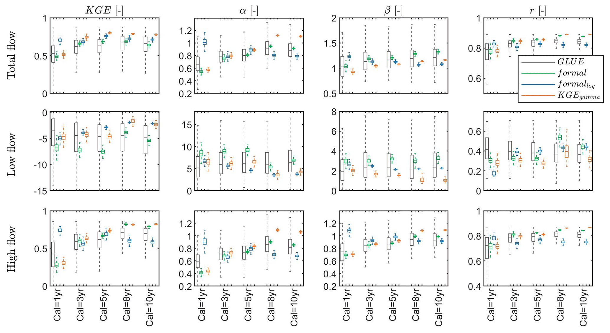
Figure 7General performance (KGE), variability (α), non-scaled bias (β) and correlation (r) for total flow, low flow (smaller than 10th percentile of observed discharge) and high flow (larger than 90th percentile of observed discharge) during the evaluation period using the GLUE approach (GLUE), the formal likelihood function (formal), the log-transformation (formallog) and our approach using KGE and gamma distribution to derive probability density (KGEgamma) with varying amounts of observations (1-year to 10-year) in calibration, for instance, calibration with 1-year observations is shown as Cal = 1 yr. The boxplot shows the performance of the last 25 % of all simulations (top 25 % in performance for GLUE), which is used to approximate the “true” system behavior in DREAM(ZS). The performance is only shown for the evaluation period to avoid too much information in the boxplot and to represent the prediction ability of different approaches. The performance of the calibration period is provided in Fig. S1 in the Supplement. The optimal value for KGE, α, β and r is 1, and the closer to 1 the better the performance.
In this section, we focus on analyzing the performance in the evaluation period to show the prediction ability of the four approaches. Generally, the uncertainty of the model performance (represented by the interquartile of KGE, α, β and r) of the GLUE approach is much larger than the other three approaches (Fig. 7) regardless of total flow, low flow or high flow. With the increasing amount of observations added to calibrations, the performance of GLUE does not change significantly for all four metrics and for all flow conditions, while using the adapted KGE or the formal likelihood function we can see an increasing trend of the model performance. The log-transformation only has an improved performance regarding low flow with increasing observation data. In the following, we focus on comparing the performance between the adapted KGE, the formal likelihood function and the log-transformation. The log-transformation has a better performance for low flow as expected, but a lower performance for high flow. The formal likelihood function without transformation has a better performance for high flow but a lower performance for low flow. The adapted KGE combines these advantages, leading to a good and balanced performance for low and high flows. For the total flow, the general performance KGE of our approach is higher than using the other two formal likelihood functions. The three approaches perform similarly for the variability (α) for calibrations with 3–5 years of data, while the adapted KGE tends to overestimate and the other two formal likelihood functions underestimate variability when more data are added to calibrations. The adapted KGE has a smaller overestimation of bias (β) than the formal likelihood functions. They have similar performance in terms of the correlation (r) for the total flow. For the low flow, the performances (all metrics) of all three approaches are poor. The adapted KGE and the log-transformation have a similar general performance in KGE, which is better than the formal likelihood function without log-transformation. The adapted KGE has a lower overestimation of variability and a better simulation of bias, while the two formal likelihood functions have a better performance in correlation. For the high flow, the adapted KGE and the formal likelihood function perform similarly in terms of KGE, bias (β) and correlation (r), which are both better than the log-transformation but the adapted KGE has a better representation of variability (α) than the two formal likelihood functions.

Figure 8General performance (KGE), variability (α), non-scaled bias (β) and correlation (r) for discharge and solutes (Cl−, and ) for a heterogeneous karst system using the formal likelihood function with normalized observations (formalnorm), the formal likelihood function with equal weights of normalized discharge and each solute (formalnorm,w) and our approach using KGE and gamma distribution to derive probability density (KGEgamma). The boxplot shows the performance of the last 25 % of all simulations, which is used to approximate the “true” system behavior in DREAM(ZS). The optimal value for KGE, α, β and r is 1, and the closer to 1 the better the performance.
3.3 Case study 3: model parameter calibrations for a heterogeneous karst system
For calibration combining discharge and solute concentrations at this heterogeneous karst system with short observation records, the adapted KGE is superior than the formal likelihood function regardless of the weight given to discharge and solutes (Fig. 8). For the general performance measured by KGE, the adapted KGE approach performs best, followed by the formal likelihood function with same weights in discharge and each solute, and then the calibration with different weights (the number of discharge data is 10 times for each solute). The performance regarding discharge is similar between the three approaches (the mean KGE is around 0.9) with a slightly higher performance for the adapted KGE approach. However, the adapted KGE approach improves the mean performance regarding Cl−, and by 7 %, 10 % and 44 %, respectively, compared to the formal likelihood function using discharge and solutes. The adapted KGE approach has a very good representation of variability (α) compared to the other two approaches, especially for discharge, Cl− and where the variability metric α is centered around 1. The performance in terms of bias (β) is in the range of 0.9 and 1.1 for all 3 approaches. The correlations of simulated and observed discharges are all larger than 0.9 for the three approaches but the adapted KGE and the formal likelihood function using the same weight in discharge and solutes have a higher performance (improvement is up to 17 %) regarding correlation for the three solutes compared with the formal likelihood function using different amounts of observation data.
As the formal likelihood function with the same weight for discharge and solutes (formalnorm,w) has a better performance than the formal likelihood function with different amounts of observation data for discharge and solutes (formalnorm), we only show the comparison regarding the total uncertainty between formalnorm,w and KGEgamma in Fig. 9. The two approaches have a similar uncertainty estimate (both total uncertainty in Fig. 9 and parameter uncertainty in Fig. S2) for discharge and . However, the formalnorm,w approach has a large underestimation for Cl− and compared to the adapted KGE approach even though the uncertainty width is similar. From Fig. 9, we can see that the adapted KGE approach can cover most very high and very low concentration values in the total uncertainty band. For the parameter uncertainty (Fig. S2), the adapted KGE approach performs better for Cl− and as well. This indicates that the adapted KGE approach can better represent the uncertainty when using multiple types of data for calibration such as discharge and three solutes in this case study.
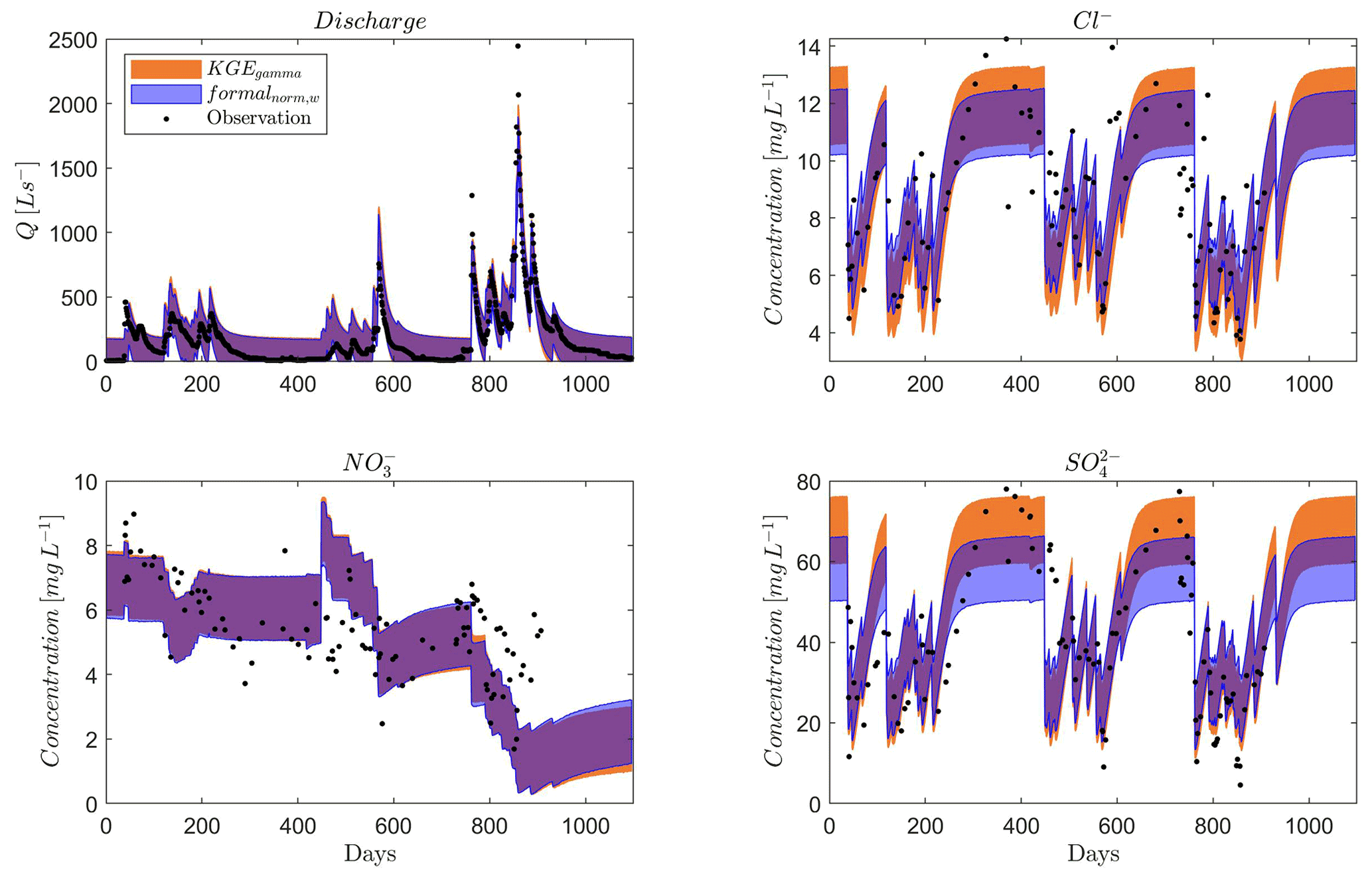
Figure 9Total uncertainty for discharge and solutes (Cl−, and ) for a heterogeneous karst system using the formal likelihood function with equal weights of normalized discharge and each solute (formalnorm,w) and our approach using KGE and gamma distribution to derive probability density (KGEgamma). The total uncertainty is estimated based on the last 25 % of all simulations. The parameter uncertainty is shown in Fig. S2.
Using the original KGE as the likelihood function, model parameters are not easily identifiable, which results in a very large uncertainty in the simulation. This is because directly using the original KGE as the likelihood estimate assumes a linear increase of probability density with the linear increase of KGE. It leads to the identification of parameter proposals with good KGE performance to be more difficult and inefficient. The difference between large and small KGE values is not distinctly large enough that the probability to accept poor proposals is high. This is why we find a very large acceptance rate and a very fast convergence rate. Mantovan and Todini (2006) and Stedinger et al. (2008) also mentioned that using the informal likelihood function, such as Nash-Sutcliffe efficiency (NSE), in the generalized likelihood uncertainty estimation (GLUE) as objectives cannot find proper posterior distributions of model parameters. Therefore, directly using the original KGE should be avoided and some adaptations to solve the incapability of exploring the posterior distributions such as our approach are needed in MCMC methods.
The adapted KGE can make a good estimate of the pseudo-analytical posterior distributions of model parameters derived from the formal likelihood function in case study 1. This suggests that it is capable of exploring the parameter posterior distributions. The adapted KGE has a lower acceptance rate and convergence rate compared to the formal likelihood function for the virtual experiment (case study 1). The possible reason is that one KGE value can cover multiple error combinations with the same RMSE around the true optimum, which makes the RMSE slightly more efficient at drawing proposals for parameters very close to the true optimum (known parameters in case study 1) for a system that only contains little uncertainty. However, calibrations of real systems usually contain more uncertainties e.g., uncertainties in forcing (including the spatial averaging), observation data (measurement errors), and uncertainty in model structures. The adapted KGE has a similar convergence rate (efficiency) as the formal likelihood for the real-world calibrations (case study 2). In particular, the acceptance rate of the adapted KGE is around 20 % for a system where we have good input and observations (case study 2). This is similar to the formal likelihood function and is also close to the theoretically optimal acceptance rate (0.234) in Metropolis algorithms with random walk (Yang et al., 2020).
The uncertainty bound of discharge simulations in case study 1 is almost identical between the adapted KGE and the formal likelihood function. This indicates that our approach can behave similarly concerning discharge uncertainty estimation as the formal likelihood function. For the calibration to the real system, the adapted KGE even has a higher general performance in terms of the mean KGE of the evaluation for the total, low and high flows than the formal likelihood function and the log-transformation. McMillan and Clark (2009) had a similar finding that using another informal likelihood function, NSE, in MCMC methods outperforms the formal likelihood for calibrations with high variability and multiple optima. The formal likelihood functions go along with the strong assumption that errors are distributed normally (Vrugt et al., 2008, 2009), the informal likelihood function KGE takes into account more variability without strict assumptions on error sources (Gupta et al., 2009). The adapted KGE performs similar to the formal likelihood function regarding the correlation between simulations and observations shown in case study 2. However, they all have lower performance for the low flow simulations compared to the total and high flow simulations. While the log-transformation works well for low flow (case study 2), the adapted KGE has a good and balanced performance for both high and low flows. It also shows a lower overestimation of bias in low flows shown as the metric β in case study 2. Jeannin et al. (2021) found that using formal likelihood functions such as RMSE as objectives has a large bias in base flow simulations. For RMSE as the objective, each individual error has the same weight. To have a high overall performance, the optimization tends to firstly fit the high flows as its error is relatively larger and the contribution to RMSE is thus larger. The log-transformation can improve the calibration for low values but is not good for high values. The adapted KGE and the formal likelihood function both have a better representation of variability (α) with more observations included in calibrations. This makes sense because when more data are involved in calibration more information on variability will be captured in calibrations.
While our approach has a similar performance as the formal likelihood function for discharge simulations, we find similar posterior distributions for certain parameters but also inconsistent posterior distributions for some parameters between the formal and informal approaches. This is because some model processes interplay with other processes such that there is compensation of one parameter for another, i.e., parameter interactions. Adding additional information, e.g., solutes in case study 3, can help to further constrain model parameters (Hartmann et al., 2017) and represents the complexity of real hydrological systems. Our study shows that the adapted KGE approach is superior for simultaneously calibrating model parameters with different types of data than the formal likelihood function. This can improve the model calibration using the traditional separate steps such as firstly calibrating discharge and then solute processes in Liu et al. (2020). Many studies have shown that multi-objective calibrations allow important characteristics of a system to be adequately and properly estimated (Vrugt et al., 2003b; Yapo et al., 1998). Using KGE can provide a feasible way to combine various types of observations as a measure of multi-objective performance and avoid issues regarding data units, scales and frequency.
Even though our approach adapts the gamma distribution to compute the probability density for KGE, the way we formulate the likelihood function based on KGE is still informal. It means the derivation of the likelihood is not from a strict theoretical probability framework, which is a limitation of our approach. Nevertheless, our approach provides a feasible and pragmatic way and a close solution to the formal likelihood function to avoid the pitfalls of directly using the original KGE in MCMC methods. Future work is needed to find a solution to link probability density and KGE in order to incorporate KGE in a statistical manner as much as possible.
Our study demonstrates that using the original KGE in DREAM(ZS) results in a very high acceptance rate and a large uncertainty bound of discharge simulations. This is due to the confusing evolution orientation for negative KGE values and the nonlinear performance of KGE. To solve these two problems, we propose adapting KGE with the gamma distribution to formulate the pseudo log-likelihood function to avoid negative posterior density ratios and to include a proper nonlinearity of performance. With three case studies we demonstrate that the adapted KGE performs as well as the formal likelihood function for the exploration of the posterior distributions of model parameters. Through the calibrations varying the amount of observations included in the calibration, we show that the adapted KGE is robust and has a good and balanced performance for both low and high flows compared to the formal likelihood function and the log-transformation. Our approach even has a higher general performance, the mean KGE of the evaluation, and a smaller bias overestimation of low flows than the formal likelihood function. Our study shows that the adapted KGE approach outperforms the formal likelihood function for calibrations using discharge and solutes. The limitation of our approach is the lack of theoretical probability derivation. Besides that formal limitation, our approach keeps the advantages of KGE, e.g., consideration of variability and possibilities to combine multiple types of data, and performs like a pseudo formal likelihood. Thus, it provides a feasible way to use KGE as an informal likelihood function in MCMC methods.
All data used in this study have been published in Liu et al. (2021) and Hartmann, et al. (2014) and the dataset is publicly available described by Newman et al. (2015) and Addor et al. (2017) and can be accessed via Newman et al. (2014) (https://doi.org/10.5065/D6MW2F4D). The Matlab code for using our approach to calculate the likelihood is provided in the Supplement.
The supplement related to this article is available online at: https://doi.org/10.5194/hess-26-5341-2022-supplement.
YL conceptualized the study, developed and applied the adapted KGE approach, and visualized the results. YL and JFO wrote the paper, and analyzed the results. MM and AH provided supervision and advice throughout developing the adapted KGE approach and supported the development of this manuscript. All authors contributed to the revision of the manuscript.
The contact author has declared that none of the authors has any competing interests.
Publisher's note: Copernicus Publications remains neutral with regard to jurisdictional claims in published maps and institutional affiliations.
We thank Jasper A. Vrugt for his constructive comments and suggestions. We thank the editor, Jiangjiang Zhang and another anonymous reviewer for their valuable comments during the peer-review phase. Yan Liu and Andreas Hartmann were supported by the Emmy-Noether-Programme of the German Research Foundation (DFG, grant number: HA 8113/1-1, project “Global Assessment of Water Stress in Karst Regions in a Changing World”). Jaime Fernández-Ortega and Matías Mudarra were supported by the European Project “Karst Aquifer Resources availability and quality in the Mediterranean Area (KARMA)” PRIMA, ANR-18-PRIM-0005 (PCI2019-103675), and by the project PID2019-111759RB-I00 funded by the Spanish Research Agency. Additionally, it is a contribution to the Research Group RNM-308 of Junta de Andalucía. Jaime Fernández-Ortega was also supported by the Erasmus+ Programme of the European Commission.
This research has been supported by the Deutsche Forschungsgemeinschaft (grant no. HA 8113/1-1), the Agencia Estatal de Investigación (grant no. PID2019-111759RB-I00), the Horizon 2020 ((4PRIMA) grant no. 724060).
This open-access publication was funded by the University of Freiburg.
This paper was edited by Lelys Bravo de Guenni and reviewed by Jiangjiang Zhang and one anonymous referee.
Addor, N., Newman, A. J., Mizukami, N., and Clark, M. P.: The CAMELS data set: catchment attributes and meteorology for large-sample studies, Hydrol. Earth Syst. Sci., 21, 5293–5313, https://doi.org/10.5194/hess-21-5293-2017, 2017.
Beven, K. J., Smith, P. J., and Freer, J. E.: So just why would a modeller choose to be incoherent?, J. Hydrol., 354, 15–32, https://doi.org/10.1016/j.jhydrol.2008.02.007, 2008.
Freer, J., Beven, K., and Ambroise, B.: Bayesian Estimation of Uncertainty in Runoff Prediction and the Value of Data: An Application of the GLUE Approach, Water Resour. Res., 32, 2161–2173, https://doi.org/10.1029/95WR03723, 1996.
Gupta, H. V., Kling, H., Yilmaz, K. K., and Martinez, G. F.: Decomposition of the mean squared error and NSE performance criteria: Implications for improving hydrological modelling, J. Hydrol., 377, 80–91, https://doi.org/10.1016/j.jhydrol.2009.08.003, 2009.
Hartmann, A., Mudarra, M., Andreo, B., Marín, A., Wagener, T., and Lange, J.: Modeling spatiotemporal impacts of hydroclimatic extremes on groundwater recharge at a Mediterranean karst aquifer, Water Resour. Res., 50, 6507–6521, https://doi.org/10.1002/2014WR015685, 2014.
Hartmann, A., Antonio Barberá, J., and Andreo, B.: On the value of water quality data and informative flow states in karst modelling, Hydrol. Earth Syst. Sci., 21, 5971–5985, https://doi.org/10.5194/hess-21-5971-2017, 2017.
Jeannin, P.-Y., Artigue, G., Butscher, C., Chang, Y., Charlier, J.-B., Duran, L., Gill, L., Hartmann, A., Johannet, A., Jourde, H., Kavousi, A., Liesch, T., Liu, Y., Lüthi, M., Malard, A., Mazzilli, N., Pardo-Igúzquiza, E., Thiéry, D., Reimann, T., Schuler, P., Wöhling, T., and Wunsch, A.: Karst modelling challenge 1: Results of hydrological modelling, J. Hydrol., 600, 126508, https://doi.org/10.1016/j.jhydrol.2021.126508, 2021.
Knoben, W. J. M., Freer, J. E., and Woods, R. A.: Technical note: Inherent benchmark or not? Comparing Nash–Sutcliffe and Kling–Gupta efficiency scores, Hydrol. Earth Syst. Sci., 23, 4323–4331, https://doi.org/10.5194/hess-23-4323-2019, 2019.
Lindström, G., Johansson, B., Persson, M., Gardelin, M., and Bergström, S.: Development and test of the distributed HBV-96 hydrological model, J. Hydrol., 201, 272–288, https://doi.org/10.1016/S0022-1694(97)00041-3, 1997.
Liu, Y., Zarfl, C., Basu, N. B., and Cirpka, O. A.: Modeling the Fate of Pharmaceuticals in a Fourth-Order River Under Competing Assumptions of Transient Storage, Water Resour. Res., 56, e2019WR026100, https://doi.org/10.1029/2019WR026100, 2020.
Liu, Y., Wagener, T., and Hartmann, A.: Assessing Streamflow Sensitivity to Precipitation Variability in Karst-Influenced Catchments With Unclosed Water Balances, Water Resour. Res., 57, e2020WR028598, https://doi.org/10.1029/2020WR028598, 2021.
Mantovan, P. and Todini, E.: Hydrological forecasting uncertainty assessment: Incoherence of the GLUE methodology, J. Hydrol., 330, 368–381, https://doi.org/10.1016/j.jhydrol.2006.04.046, 2006.
McInerney, D., Thyer, M., Kavetski, D., Lerat, J., and Kuczera, G.: Improving probabilistic prediction of daily streamflow by identifying Pareto optimal approaches for modeling heteroscedastic residual errors, Water Resour. Res., 53, 2199–2239, https://doi.org/10.1002/2016WR019168, 2017.
McMillan, H. and Clark, M.: Rainfall-runoff model calibration using informal likelihood measures within a Markov chain Monte Carlo sampling scheme, Water Resour. Res., 45, 1–12, https://doi.org/10.1029/2008WR007288, 2009.
Newman, A., Sampson, K., Clark, M. P., Bock, A., Viger, R. J., and Blodgett, D.: A large-sample watershed-scale hydrometeorological dataset for the contiguous USA, UCAR/NCAR [data set], https://doi.org/10.5065/D6MW2F4D, 2014.
Newman, A. J., Clark, M. P., Sampson, K., Wood, A., Hay, L. E., Bock, A., Viger, R. J., Blodgett, D., Brekke, L., Arnold, J. R., Hopson, T., and Duan, Q.: Development of a large-sample watershed-scale hydrometeorological data set for the contiguous USA: Data set characteristics and assessment of regional variability in hydrologic model performance, Hydrol. Earth Syst. Sci., 19, 209–223, https://doi.org/10.5194/hess-19-209-2015, 2015.
Pool, S., Vis, M., and Seibert, J.: Evaluating model performance: towards a non-parametric variant of the Kling–Gupta efficiency, Hydrolog. Sci. J., 63, 1941–1953, https://doi.org/10.1080/02626667.2018.1552002, 2018.
Smith, T. J. and Marshall, L. A.: Bayesian methods in hydrologic modeling: A study of recent advancements in Markov chain Monte Carlo techniques, Water Resour. Res., 44, 1–9, https://doi.org/10.1029/2007wr006705, 2008.
Stedinger, J. R., Vogel, R. M., Lee, S. U., and Batchelder, R.: Appraisal of the generalized likelihood uncertainty estimation (GLUE) method, Water Resour. Res., 44, 1–17, https://doi.org/10.1029/2008wr006822, 2008.
Vrugt, J. A.: Markov chain Monte Carlo simulation using the DREAM software package: Theory, concepts, and MATLAB implementation, Environ. Model. Softw., 75, 273–316, https://doi.org/10.1016/j.envsoft.2015.08.013, 2016.
Vrugt, J. A., Gupta, H. V., Bouten, W., and Sorooshian, S.: A Shuffled Complex Evolution Metropolis algorithm for optimization and uncertainty assessment of hydrologic model parameters, Water Resour. Res., 39, 1201, https://doi.org/10.1029/2002WR001642, 2003a.
Vrugt, J. A., Gupta, H. V., Bastidas, L. A., Bouten, W., and Sorooshian, S.: Effective and efficient algorithm for multiobjective optimization of hydrologic models, Water Resour. Res., 39, 1–19, https://doi.org/10.1029/2002WR001746, 2003b.
Vrugt, J. A., Ter Braak, C. J. F., Clark, M. P., Hyman, J. M., and Robinson, B. A.: Treatment of input uncertainty in hydrologic modeling: Doing hydrology backward with Markov chain Monte Carlo simulation, Water Resour. Res., 44, W00B09, https://doi.org/10.1029/2007WR006720, 2008.
Vrugt, J. A., Ter Braak, C. J. F., Diks, C. G. H., Robinson, B. A., Hyman, J. M., and Higdon, D.: Accelerating Markov chain Monte Carlo simulation by differential evolution with self-adaptive randomized subspace sampling, Int. J. Nonlin. Sci. Numer. Simul., 10, 273–290, 2009.
Yang, J., Roberts, G. O., and Rosenthal, J. S.: Optimal scaling of random-walk metropolis algorithms on general target distributions, Stoch. Process. Appl., 130, 6094–6132, https://doi.org/10.1016/j.spa.2020.05.004, 2020.
Yapo, P. O., Gupta, H. V., and Sorooshian, S.: Multi-objective global optimization for hydrologic models, J. Hydrol., 204, 83–97, https://doi.org/10.1016/S0022-1694(97)00107-8, 1998.