the Creative Commons Attribution 4.0 License.
the Creative Commons Attribution 4.0 License.
 | 19 Oct 2022
A robust upwind mixed hybrid finite element method for transport in variably saturated porous media
Hussein Hoteit
Rainer Helmig
Marwan Fahs
The mixed finite element (MFE) method is well adapted for the simulation of fluid flow in heterogeneous porous media. However, when employed for the transport equation, it can generate solutions with strong unphysical oscillations because of the hyperbolic nature of advection. In this work, a robust upwind MFE scheme is proposed to avoid such unphysical oscillations. The new scheme is a combination of the upwind edge/face centered finite volume method with the hybrid formulation of the MFE method. The scheme ensures continuity of both advective and dispersive fluxes between adjacent elements and allows to maintain the time derivative continuous, which permits employment of high-order time integration methods via the method of lines (MOL).
Numerical simulations are performed in both saturated and unsaturated porous media to investigate the robustness of the new upwind MFE scheme. Results show that, contrarily to the standard scheme, the upwind MFE method generates stable solutions without under and overshoots. The simulation of contaminant transport into a variably saturated porous medium highlights the robustness of the proposed upwind scheme when combined with the MOL for solving nonlinear problems.
- Article
(2744 KB) - Full-text XML
- BibTeX
- EndNote


The mixed finite element (MFE) method (Raviart and Thomas, 1977; Brezzi et al., 1985; Chavent and Jaffré, 1986; Brezzi and Fortin, 1991; Younes et al., 2010) is known to be a robust numerical scheme for solving elliptic diffusion problems such as the fluid flow in heterogeneous porous media. The method combines advantages of the finite volumes, by ensuring local mass conservation and continuity of fluxes between adjacent cells, and advantages of finite elements by easily handling heterogeneous domains with discontinuous parameter distributions and unstructured meshes. As a consequence, the MFE method has been largely used for flow in porous media (see, for instance, the review of Younes et al. (2010) and references therein). The hybridization technique has been largely used with the MFE method to improve its efficiency (Chavent and Roberts, 1991; Traverso et al., 2013). This technique allows to reduce the total number of unknowns and produces a final system with a symmetric positive definite matrix. The unknowns with the hybrid MFE method are the Lagrange multipliers which correspond to the traces of the scalar variable at edges/faces (Chavent and Jaffré, 1986).
When applied to transient diffusion equations with small time steps, the hybrid MFE method can produce solutions with small unphysical over- and undershoots (Hoteit et al., 2002a, b; Mazzia, 2008). A lumped formulation of the hybrid MFE method was developed by Younes et al. (2006) to improve its monotonicity and reduce nonphysical oscillations. The lumped formulation ensures that the maximum principle is respected for parabolic diffusion equations on acute triangulations (Younes et al., 2006). For more general 2D and 3D element shapes, the lumping procedure allows to significantly improve the monotonous character of the hybrid MFE solution (Younes et al., 2006; Koohbor et al., 2020). As an illustration, the lumped formulation was shown to be more efficient and more robust than the standard hybrid formulation for the simulation of the challenging nonlinear problem of water infiltration into an initially dry soil (Belfort et al., 2009). The lumped formulation has recently been used for flow discretization in the case of density-driven flow in saturated–unsaturated porous media (Younes et al., 2022a).
However, the MFE method remains little used for the discretization of the full transport equation. When employed to the advection–dispersion equation, the MFE method can generate solutions with strong numerical instabilities in the case of advection-dominated transport because of the hyperbolic nature of the advection operator. To avoid these instabilities, one of the most popular and easiest ways is to use an upwind scheme. Indeed, although upwind schemes introduce some numerical diffusion leading to an artificial smearing of the numerical solution, they avoid unphysical oscillations and remain useful, especially for large domains and regional field simulations. In the literature, some upwind mixed finite element schemes have been employed to improve the robustness of the MFE method for advection-dominated problems (Dawson, 1998; Dawson and Aizinger, 1999; Radu et al., 2011; Vohralík, 2007; Brunner et al., 2014).
The main idea of an upwind scheme for an element E is to calculate the mass flux exchanged with its adjacent element E′ using the concentration from E in the case of an outflow and the concentration from E′ in the case of an inflow. However, this idea cannot be applied as such with the hybrid MFE method since the hybridization procedure requires to express the flux at the element interface as only a function of variables at the element E (and not E′). To overcome this difficulty, Radu et al. (2011) and Brunner et al. (2014) proposed an upwind MFE method where, in the case of an inflow, the concentration at the adjacent element E′ is replaced by an approximation using the concentration at E and the trace of concentration at the interface by assuming that the edge concentration is the mean of the concentrations in E and E′. However, this assumption cannot be verified for a general configuration. Furthermore, with such an assumption, each of the advective and dispersive fluxes is discontinuous at the element interfaces, and continuity is only fulfilled for the total flux.
In this work, a new upwind MFE method is proposed for solving the full transport equation without requiring any approximation of the upwind concentration. The new scheme is a combination of the upwind edge/face centered finite volume (FV) scheme with the lumped formulation of the MFE method. It guarantees continuity of both advective and dispersive fluxes at element interfaces. Further, the new upwind MFE scheme maintains the time derivative continuous, and thus allows to employ high-order time integration methods via the method of lines (MOL), which was shown to be very efficient for solving nonlinear problems (see, for instance, Fahs et al., 2009 and Younes et al., 2009).
This article is structured as follows. In Sect. 2, we recall the hybrid MFE method for the discretization of the transport equation. In Sect. 3, we introduce the new upwind MFE method based on the combination of the upwind edge/face FV scheme with the lumped formulation of the MFE method. In Sect. 4, numerical experiments are performed for transport in saturated and unsaturated porous media to investigate the robustness of the new developed upwind MFE scheme. Some conclusions are given in the last section of the article.
The mass conservation of the contaminant in variably saturated porous media is
where C is the normalized concentration [–], θ is water content [L3 L−3], t is time [T], is the advective flux with q the Darcy velocity [L T−1], and the dispersive flux given by
with D, the dispersion tensor, expressed by
in which αL and αT are the longitudinal and transverse dispersivities [L], Dm is the pore water diffusion coefficient [L2 T−1], and I is the unit tensor.
The water content θ and the Darcy velocity q are linked by the fluid mass conservation equation in variably saturated porous media:
Substituting Eq. (4) into Eq. (1) yields the following advection–dispersion equation:
In this work, we consider that the velocity q is obtained by solving Richards' equation using the hybrid MFE method. For a two-dimensional domain with a triangular mesh, q is approximated inside each triangle E using the lowest-order Raviart–Thomas (RT0) vectorial basis functions :
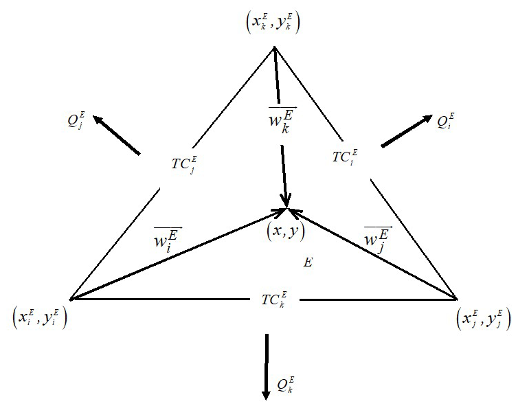
where is the water flux across the edge Ej of E (see Fig. 1) and is the typical RT0 basis functions (Younes et al., 1999) with the coordinates of the node j opposite to the edge Ej of E, and the area of E.
To apply the hybrid MFE method to the transport Eq. (5), we approximate the dispersive flux with RT0 vectorial basis functions as
where is the dispersive flux across the edge Ej of the element E and is the outward unit normal vector to the edge Ej.
The variational formulation of Eq. (2) using the test function yields
Substituting Eq. (7) into Eq. (8) and using properties of the basis functions give
in which DE is the local dispersion tensor at the element E, CE is the mean concentration at E, and TC is the edge (trace) concentration (Lagrange multiplier) at the edge Ei.
Denoting the local matrix , the inversion of the system of Eq. (9) gives the expression for the dispersive flux :
Besides, the integration of the mass conservation Eq. (6) over the element E writes
which becomes, using Green's formula,
where θE is the water content of the element E.
Substituting Eq. (2) into Eq. (12) yields
in which is the total flux at the edge Ei with the advective flux given by and the dispersive flux given by Eq. (10).
The hybridization of the MFE method is performed in the following two steps.
The flux Eq. (10) is substituted into the mass conservation Eq. (13), which is then discretized in time using the first-order implicit Euler scheme,
in which and .
Hence, the mean concentration at the new time level can be expressed as a function of , the concentration at the edges of E, as follows:
in which and .
The mean concentration given by Eq. (15) is then substituted into the flux Eq. (10), which allows expressing the dispersive flux (the subscript n+1 will be omitted to alleviate the notations) as only a function of the traces of concentration at edges :
The system to be solved is obtained by imposing the continuity of the total flux as well as the continuity of the trace of concentration at the edge i between the two elements E and E′ (Fig. 2).
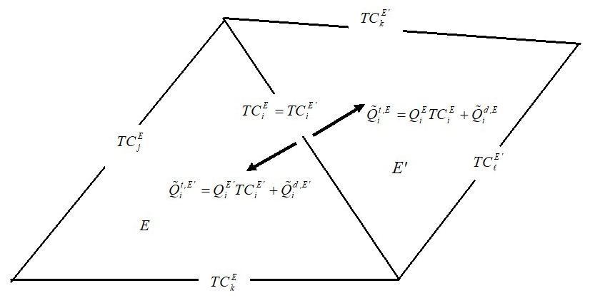
Figure 2Continuity of concentration and total flux between adjacent elements with the hybrid MFE method.
Note that the advective flux is continuous between E and E′ because of the continuity of the water flux and the continuity of the trace of concentration at the interface. Thus, for the continuity of the total flux , it is required that the dispersive flux is continuous:
Using Eq. (16), we obtain
The continuity Eq. (18) is written for all mesh edges, and the resulting equations form the final system to be solved for the traces of concentration at edges as unknowns.
Note that the hybrid MFE Eq. (18), obtained by approximating the dispersive flux with RT0 basis functions, is equivalent to the new MFE method proposed in Radu et al. (2011).
In this section, we recall the main principles of two existing approaches, developed to improve the stability of the MFE solution of the transport equation. The first approach is the upwind hybrid MFE scheme of Radu et al. (2011), developed for advection dominated transport. The second approach is the lumped hybrid MFE method of Younes et al. (2006), developed for dispersive transport.
3.1 The upwind hybrid MFE of Radu et al. (2011)
In the case of advection-dominated transport, solving the hybrid MFE Eq. (18) can yield solutions with strong instabilities. A common way to avoid such instabilities is to use an upwind scheme for the advective flux. Thus, for an element E, the advective flux at the edge i (common with the element E′) has to be calculated using either the concentration from E (if ) or the concentration from E′ (if ). Radu et al. (2011) suggested replacing the advective flux at the interface by
The advective term is now calculated using the upwind mean concentration, which can be that of the element E or of its adjacent element E′.
The advective flux of Eq. (19) is rewritten in the following condensed form:
with for an outflow and for an inflow .
However, this expression is incompatible with the hybridization procedure. Indeed, if we replace, in the Eq. (14), the advective term by Eq. (20), the latter will contain both CE and . Thus, the first step of the hybridization procedure cannot allow expressing as only a function of as in the Eq. (15).
To avoid this difficulty, Radu et al. (2011) suggested replacing by the following expression:
This approximation is based on the assumption that .
Plugging Eq. (21) into Eq. (20), the advective flux depends only on the variables of the element E (mean concentration CE and edge concentration ):
Equation (22) can then be used to replace the advective term in Eq. (14), and thus the hybridization procedure allows to express as a function of as in the Eq. (15). Then, the expression of is substituted into the dispersive flux Eq. (10), and the final system is obtained by prescribing continuity of the total flux at the interface between E and E′. This scheme was shown to be more efficient (by using a sparser system matrix with fewer unknowns) than the non-hybrid upwind mixed method of Dawson (1998). The two methods yielded optimal first-order convergence in time and space (Brunner et al., 2014).
The assumption given by Eq. (21) can be a rough approximation, especially in the case of a heterogeneous domain where dispersion can vary with several orders of magnitudes from element to element. For such a situation, the edge concentration can be significantly different from the average of the mean concentrations of adjacent elements. Furthermore, the advective flux is not uniquely defined at the interface and can be different for the two adjacent elements E and E′. For instance, in the case of , the advective flux leaving the element E is , whereas the flux entering the element E′ is which could be different as is not necessarily the mean of CE and . In this situation, because of the discontinuity of the advective flux, the dispersive flux will not be continuous at the interface since the continuity is prescribed only for the total flux.
3.2 The lumped hybrid MFE scheme for dispersion transport
In this section, we recall the main principles of the lumped hybrid MFE method of Younes et al. (2006), developed to improve the stability of the MFE solution in the case of dispersive transport.
Considering only dispersion, Eq. (5) simplifies to
As detailed above, the hybrid MFE method for Eq. (23) is based on two stages:
Stage 1. Discretization of the transient mass conservation equation over the element E: the integration of the mass conservation Eq. (23) over the element E gives (see Eq. 13) the following:
Stage 2. Imposing the continuity of the flux across the edge i sharing the two elements E and E′:
Note that the continuity Eq. (25) can be interpreted as a steady-state mass conservation equation at the edge level. Hence, the hybrid MFE discretization uses the transient mass conservation equation at the element level, given by Eq. (24), and the steady-state mass conservation at the edge level, given by Eq. (25). With the lumped hybrid MFE method of Younes et al. (2006), the transient term is taken into account at the edge level. Hence, the lumped formulation uses a steady-state mass conservation equation at the element level and a transient mass conservation equation at the edge level. The two stages of the lumped hybrid MFE are as follows:
Stage 1. Discretization of the steady-state mass conservation equation over E: the steady-state transport over the element E writes
where is the steady-state dispersive flux across the edge Ei.
Therefore, the mean concentration of Eq. (15) becomes
and using Eq. (16), the steady-state dispersive flux writes
Stage 2. Discretization of the transient mass conservation equation over the lumping region Ri: the edge centered finite volume discretization of the transient transport Eq. (23) over the lumping region Ri (hatched area in Fig. 3), associated with the edge i, writes
where the lumping regions Ri is formed by the two simplex regions and , for an inner edge i sharing the two elements E and E′, and by the sole simplex region for a boundary edge. The simplex region is defined by joining the center of E with the nodes j and k forming the edge i.
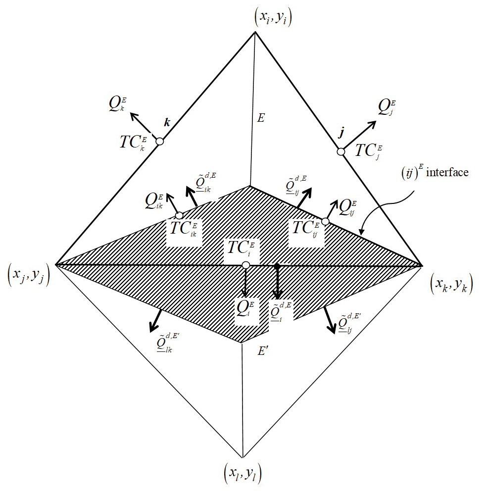
Figure 3The lumping region Ri associated with the edge i, sharing the elements E and E′, and formed by the two simplex regions and .
Associating the edge concentration to Ri (see Fig. 3 for notations), Eq. 29) gives
in which and are respectively the dispersive flux and the concentration at the interior interface (ij)E between the simplex regions and . The shortcut { }′ designates the same contribution as { }, but of the adjacent element E′, in the case of Eq. (30), it corresponds to .
Besides, applying the steady-state dispersive transport Eq. (26) on the simplex region yields
Finally, substituting Eqs. (28 ) and (31) into the transport Eq. (30) gives the final system to solve with the lumped hybrid MFE scheme:
Note that the lumped hybrid formulation Eq. (32) and the standard hybrid formulation (Eqs. 24 and 25) are exactly the same in the case of steady-state diffusion transport.
In the lumped formulation Eq. (32), the term of mass (with time derivative) has a contribution only on the diagonal term of the final system matrix. This improves the monotonous character of the solution (see Younes et al., 2006). For instance, in the case of an acute triangulation, the maximum principle is respected by the lumped formulation Eq. (32) whatever the heterogeneity of the porous medium (Younes et al., 2006).
Contrarily to the standard hybrid MFE scheme, where the discretization of the temporal derivative performed in Eq. (14) was necessary to obtain the final system given by Eq. (18), the lumped scheme given by Eq. (32) keeps the time derivative continuous which allows the use of efficient high-order temporal discretization methods via the MOL.
In the case of 2D triangular elements, the lumped formulation Eq. (32) is algebraically equivalent to the nonconforming Crouzeix–Raviart (Crouzeix and Raviart, 1973) finite element method (see Younes et al., 2008). The nonconforming Crouzeix–Raviart method uses the chapeau functions as basis functions to approximate the concentration, like the standard finite element method, but seed nodes are the midpoints of the edges.
To avoid the rough approximation (Eq. 21), we develop hereafter a new upwind MFE scheme where the advection term is calculated using upwind edge concentration instead of upwind mean concentration of the element E. The idea of the scheme is to extend the lumped hybrid MFE procedure to transport by both advection and dispersion and to use an upwind edge centered FV scheme to avoid unphysical oscillations caused by the hyperbolic nature of advection.
The integration of the whole mass conservation Eq. (5) over the lumping region Ri writes
Using notations of Fig. 3, we obtain
in which is the water flux at the interior interface (ij)E, evaluated using the RT0 approximation of the velocity given by Eq. (6), which yields
Using Eqs. (28) and (31) and denoting , Eq. (34) becomes
The interior concentration at the interface between the simplex regions and is calculated using an upwind scheme (see Fig. 3) defined by
with if , else .
Thus, the final system to solve becomes
In the case of a first-order Euler implicit time discretization, Eq. (37) becomes
where .
It is easy to see that, due to upwinding, the system matrix corresponding to Eq. (28) is always an M-matrix (a non-singular matrix with mii>0, mij≤0) in the case of transport by advection. The M-matrix property insures the stability of the scheme since it guaranties the respect of the discrete maximum principle i.e., local maxima or minima will not appear in the C solution in a domain without local sources or sinks.
Further, Eq. (37) expresses the total exchange between E and E′ and therefore reflects the continuity of the total advection–dispersion flux between them. Both advective and dispersive fluxes are continuous between the adjacent elements E and E′. The advective flux, calculated using the upwind edge concentration, is uniquely defined at the interface of the lumping region and is therefore continuous. As a consequence, the dispersive flux is also continuous between E and E′ since the total flux is continuous at the interface between them.
In this section, a first test case dealing with transport in saturated porous media is simulated with the standard hybrid MFE and the new upwind MFE schemes. The results are compared against an analytical solution in order to validate the new developed scheme and to show its robustness for solving advection-dominated transport problems compared to the standard one. The second test case deals with transport in the unsaturated zone and aims to investigate the robustness of the new scheme when combined with the MOL for solving highly nonlinear problems.
5.1 Transport in saturated porous media: comparison against a 2D analytical solution
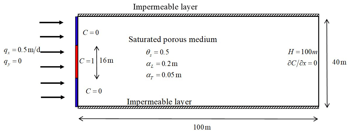
The hybrid and upwind MFE formulations are compared against the analytical solution developed by Leij and Dane (1990) for a simplified 2D transport problem (Fig. 4). The test case has been employed by Putti et al. (1990) and Siegel et al. (1997) for the verification of transport codes. It deals with the contamination from the left boundary of a 2D rectangular domain of dimension (0, 100) × (0, 40).
The boundary conditions for the transport are of Dirichlet type at the inflow (left vertical boundary), with
A zero diffusive flux is imposed at the right vertical outflow boundary. The top and bottom are impermeable boundaries. A uniform horizontal flow occurs from left to right with a constant flux qx=0.5 m d−1 prescribed at the left vertical boundary and a fixed head H=100 m at the right vertical boundary. The longitudinal and transverse dispersivities are αL=0.2 m and αT=0.05 m, respectively. The domain is discretized with a fine unstructured triangular mesh formed by 33 216 elements, and the simulation is performed for a final simulation time T=30 d using the Euler implicit time discretization with a fixed time step of 0.1 d. The linear systems are solved in each time step with a direct solver using an unsymmetric-pattern multi-frontal method and a direct sparse LU factorization (UMFPACK).
The analytical solution of this test case for an infinite domain is given by Leij and Dane (1990),
with .
The final distributions of the concentration with both hybrid MFE and upwind MFE schemes are depicted in Fig. 5. Although we have used an unstructured mesh, the two schemes yield almost symmetrical results. The hybrid MFE scheme (Fig. 5a) yields a solution with unphysical oscillations. Indeed, around 1.2 % of the contaminated region (i.e., the region with ) exhibits unphysical oscillations with 0.4 % of the contaminated region with and 0.8 % of the contaminated region with C≥1.001. These unphysical oscillations, although they seem moderate, can be dramatic, for instance, when dealing with reactive transport where some reactions occur only if the concentration exceeds a certain threshold. The solution obtained with the new upwind formulation (Fig. 5b) is monotone (all concentrations are between 0 and 1) which is in agreement with the physics. However, these results come at the expense of some numerical diffusion added to the solution. To appreciate the quality of both solutions and validate the upwind MFE method, we compare the concentration profile of the two methods to the analytical solution of Leij and Dane (1990) for a horizontal section located at y=20 m and a vertical section located at x=20 m.

Figure 5Concentration distribution with the hybrid MFE and the upwind MFE methods for the 2D saturated transport problem (only the region x≤70 m is depicted).
The results of Fig. 6 show that the solution of both hybrid MFE and upwind MFE methods are in very good agreement with the analytical solution, which validates the new upwind MFE numerical model. Note, however, that a small numerical diffusion is observed with the upwind MFE solution, which is especially visible in Fig. 6b. Indeed, for the simulated problem, the transverse dispersivity is much smaller than the longitudinal one, and, as a consequence, the concentration front is sharper in the vertical section than in the horizontal one. This explains why the numerical diffusion generated by the upwind MFE method is more pronounced in Fig. 6b than in Fig. 6a.
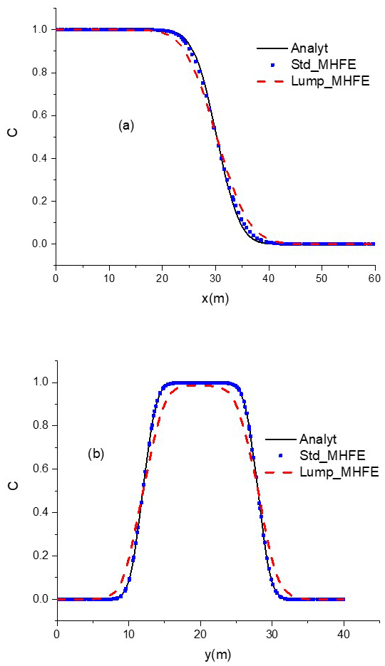
Figure 6Concentration profiles at y=20 m (a) and x=20 m (b) with the analytical, hybrid MFE, and upwind MFE solutions.
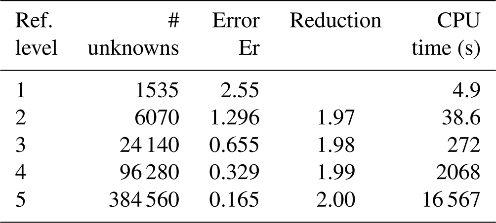
The test problem is then simulated using different mesh refinements to investigate the order of convergence of the new method. We start with a uniform mesh formed by 1000 triangles and a time step Δt=0.1 s. In each level of refinement, each triangle is subdivided into four similar triangles, by joining the three mid-edges and the time step Δt is halved. The following error is computed (Brunner et al., 2014):
where is the total advection–dispersion flux and N the total number of time steps.
The runs are performed on a single computer with an Intel Xeon E-2246G processor and 32 GB memory. The results of the computations, summarized in Table 1, clearly show optimal first-order convergence in space and time for the developed upwind hybrid MFE method.
Table 1Numerical results for the new upwind hybrid MFE method.
5.2 Transport in a variably-saturated porous medium
In this test case, the developed upwind MFE method is combined with the MOL for solving contaminant transport in a variably-saturated porous medium. The advection–dispersion equation is transformed to an ordinary differential equation (ODE) using the new upwind MFE formulation for the spatial discretization, whereas the time derivative is maintained continuously. Therefore, high-order time integration methods included in efficient ODE solvers can be employed. With these solvers, both the time step size and the order of the time integration can vary during the simulation to deliver accurate results in an acceptable computational time.
To investigate the robustness and efficiency of the combination of the developed upwind MFE method with the MOL, we simulate in this section the problem of contaminant infiltration into a variably-saturated porous medium.
The domain (Fig. 7) is a rectangular box of 3 m × 2 m, filled with sand, with an initial water table at 0.65 m and hydrostatic pressure distribution. An infiltration of a tracer contaminant is applied over the left-most 0.1 m of the surface with a constant flux of 10−6 m s−1. The right vertical side has a fixed head H=0.65 m below the water table and an impermeable boundary above it. The left vertical side and the upper (except the infiltration zone) and bottom boundaries are impermeable boundaries.
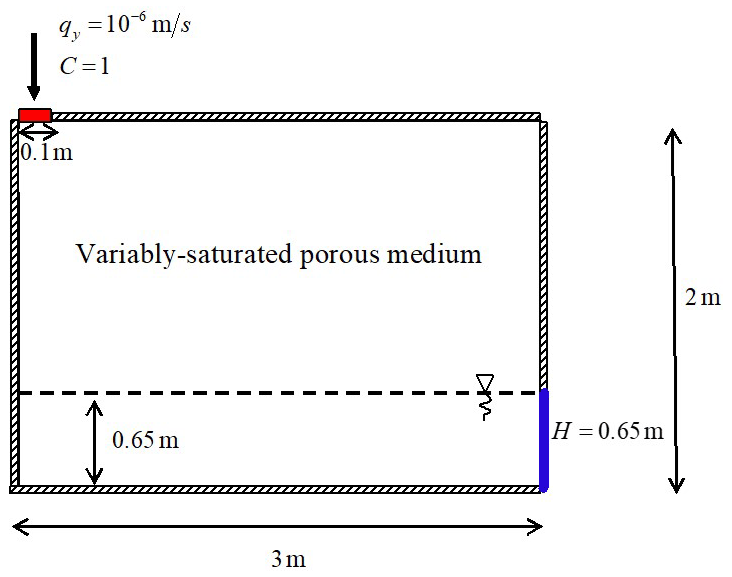
Figure 7Description of the problem of contaminant infiltration into a 2D variably-saturated porous medium.
In this problem, the flow and transport are coupled by the velocity, which is obtained by solving the following pressure-head form of the nonlinear Richards' equation:
with SS the specific mass storativity related to head changes [L−1], the equivalent head [L], the pressure head, P the pressure [Pa], ρ the fluid density [M L−3], g the gravity acceleration [L T−2], y the upward vertical coordinate [L], c(h) the specific moisture capacity [L−1], θS the saturated water content [L3 L−3], q the Darcy velocity [L T−1], the hydraulic conductivity [L T−1], k the permeability [L2], μ the fluid dynamic viscosity [M L−1 T−1], and kr the relative conductivity [–].
We use the standard van Genuchten (1980) model for the relationship between water content and pressure head,
where α [L−1] and n [–] are the van Genuchten parameters, , Se [–] is the effective saturation, and θr [–] is the residual water content. The conductivity–saturation relationship is derived from the Mualem (1976) model,
The material properties of the test problem are given in Table 2.
Table 2Parameters for the problem of infiltration into a 2D variably-saturated porous medium.
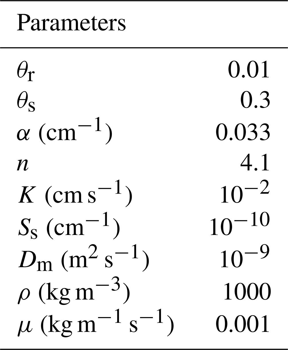
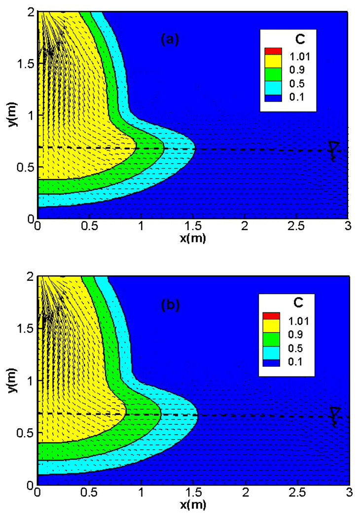
Figure 8Concentration distribution, with the hybrid MFE (a) and the upwind MFE (b) schemes for the transport problem with high dispersion in a variably-saturated porous medium.
The simulation is performed for 80 h using a triangular mesh formed by 4273 triangular elements. Two test cases are investigated. In the first test case, the longitudinal and transverse dispersivities are αL=0.03 m and αT=0.003 m, respectively. The second test case is less diffusive with αL=0.01 m and αT=0.001 m.
The coupled nonlinear flow–transport system is solved using the MOL, which allows the use of efficient high-order time integration methods, for both the hybrid MFE and the upwind MFE schemes. To this aim, a hybrid MFE formulation with continuous time derivative was developed by extending the lumping procedure, developed in Younes et al. (2006) for the flow equation, to the advection–dispersion transport Eq. (5).
The time integration is performed with the DASPK time solver which uses an efficient automatic time-stepping scheme based on the fixed leading coefficient backward difference formulas (FLCBDF). The linear systems arising at each time step are solved with the preconditioned Krylov iterative method. The nonlinear problem is linearized using the Newton method with a numerical approximation of the Jacobian matrix.
The results of the hybrid MFE and the upwind MFE methods are depicted in Fig. 8 for the first test case involving high dispersion. Good agreement can be observed between the results of the hybrid MFE (Fig. 8a) and upwind MFE (Fig. 8b) schemes when combined with the MOL. In these figures, the contaminant progresses essentially vertically through the unsaturated zone of the soil. When the saturated zone is reached, the contaminant progresses horizontally and remains close to the water table. Note that the results of both schemes are stable and free from unphysical oscillations (Fig. 8a and b).
For the second test case with lower dispersion (αL=0.01 m, αT=0.001 m), the hybrid MFE method yields unstable results containing unphysical oscillations (red color in Fig. 9a). These oscillations hamper the convergence of the numerical model, and severe convergence issues can be encountered if we further decrease the dispersivity values. The results of the upwind MFE scheme are monotone and do not contain any unphysical oscillation (Fig. 9b). These results point out the robustness of the new upwind MFE method for transport in saturated and unsaturated porous media. The developed transport scheme has recently been successfully combined with the MFE method for fluid flow to simulate nonlinear flow and transport in unsaturated fractured porous media using the 1D–2D discrete fracture matrix (DFM) approach (Younes et al., 2022b).
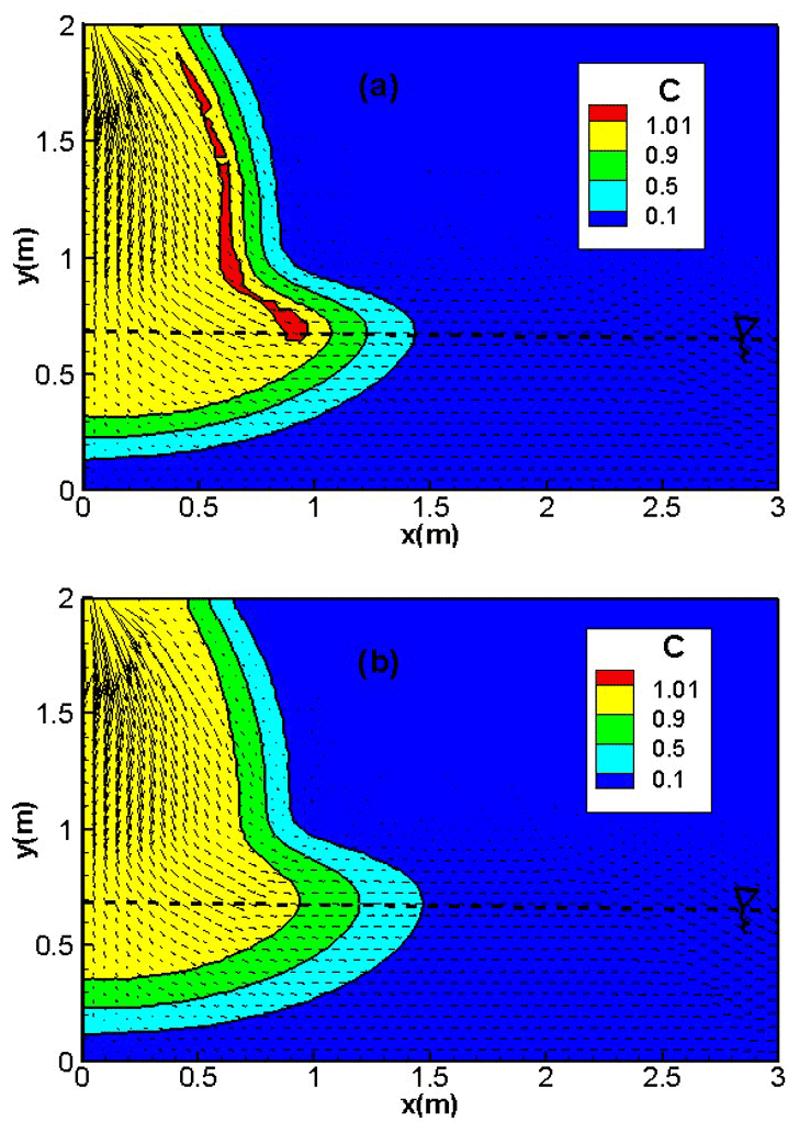
Figure 9Concentration distribution with the hybrid MFE (a) and upwind MFE (b) methods for the transport problem with low dispersion in variably-saturated porous medium.
MFE is a robust numerical method well adapted for diffusion problems on heterogeneous domains and unstructured meshes. When applied to transport equations, the MFE solution can exhibit strong unphysical oscillations due to the hyperbolic nature of advection. Upwind schemes can be used to avoid such oscillations, although they introduce some numerical diffusion. In this work, we developed an upwind scheme that does not require any approximation for the upwind concentration. The method can be seen as a combination of an upwind edge/face centered FV method with the lumped formulation of the hybrid MFE method. It ensures continuity of both advective and dispersive fluxes between adjacent elements and allows to maintain the time derivative continuous, which facilitates employment of high-order time integration methods via the method of lines (MOL) for nonlinear problems.
Numerical simulations for the transport in a saturated porous medium show that the standard hybrid MFE method can generate unphysical oscillations due to the hyperbolic nature of advection. These unphysical oscillations are completely avoided with the new upwind MFE scheme. The simulation of the problem of contaminant transport in a variably-saturated porous medium shows that only the upwind MFE scheme provides a stable solution. The results point out the robustness of the developed upwind MFE scheme when combined with the MOL for solving nonlinear transport problems.
All data presented in this paper as well as the hybrid MFE and the upwind MFE Fortran transport codes are available under request from the first author.
AY defined the aim and the conception of study, developed the numerical model, performed first numerical simulations and drafted the manuscript. HH verified the numerical model. RH revised the manuscript. MF worked on the validation of the numerical model and literature review.
The contact author has declared that none of the authors has any competing interests.
Publisher' note: Copernicus Publications remains neutral with regard to jurisdictional claims in published maps and institutional affiliations.
This paper was edited by Mauro Giudici and reviewed by Thomas Graf and two anonymous referees.
Belfort, B., Ramasomanana, F., Younes, A., and Lehmann, F.: An Efficient Lumped Mixed Hybrid Finite Element Formulation for Variably Saturated Groundwater Flow, Vadose Zone J., 8, 352–362, https://doi.org/10.2136/vzj2008.0108, 2009.
Brezzi, F. and Fortin, M. (Eds.): Mixed and Hybrid Finite Element Methods, Springer, New York, NY, https://doi.org/10.1007/978-1-4612-3172-1, 1991.
Brezzi, F., Douglas, J., and Marini, L. D.: Two families of mixed finite elements for second order elliptic problems, Numer. Math., 47, 217–235, https://doi.org/10.1007/BF01389710, 1985.
Brunner, F., Radu, F. A., and Knabner, P.: Analysis of an Upwind-Mixed Hybrid Finite Element Method for Transport Problems, SIAM J. Numer. Anal., 52, 83–102, https://doi.org/10.1137/130908191, 2014.
Chavent, G. and Jaffré, J.: Mathematical models and finite elements for reservoir simulation: single phase, multiphase, and multicomponent flows through porous media, North-Holland, Sole distributors for the U.S.A. and Canada, Elsevier Science Pub. Co, Amsterdam, New York, NY, USA, 376 pp., ISBN 9780080875385, 1986.
Chavent, G. and Roberts, J. E.: A unified physical presentation of mixed, mixed-hybrid finite elements and standard finite difference approximations for the determination of velocities in waterflow problems, Adv. Water Resour., 14, 329–348, https://doi.org/10.1016/0309-1708(91)90020-O, 1991.
Crouzeix, M. and Raviart, P. A.: Conforming and nonconforming finite element methods for solving the stationary Stokes equations, R.A.I.R.O. R3, Revue française d'automatique informatique recherche opérationnelle, Mathématique, 7, 33–76, 1973.
Dawson, C.: Analysis of an Upwind-Mixed Finite Element Method for Nonlinear contaminant Transport Equations, SIAM J. Numer. Anal., 35, 1709–1724, https://doi.org/10.1137/S0036142993259421, 1998.
Dawson, C. N. and Aizinger, V.: Upwind mixed methods for transport equations, Computat. Geosci., 3, 93–110, 1999.
Fahs, M., Younes, A., and Lehmann, F.: An easy and efficient combination of the Mixed Finite Element Method and the Method of Lines for the resolution of Richards' Equation, Environ. Model. Softw., 24, 1122–1126, https://doi.org/10.1016/j.envsoft.2009.02.010, 2009.
Hoteit, H., Mosé, R., Philippe, B., Ackerer, P., and Erhel, J.: The maximum principle violations of the mixed-hybrid finite-element method applied to diffusion equations: Mixed-hybrid finite element method, Int. J. Numer. Meth. Eng., 55, 1373–1390, https://doi.org/10.1002/nme.531, 2002a.
Hoteit, H., Erhel, J., Mosé, R., Philippe, B., and Ackerer, P.: Numerical Reliability for Mixed Methods Applied to Flow Problems in Porous Media, Comput. Geosci., 6, 161–194, 2002b.
Koohbor, B., Fahs, M., Hoteit, H., Doummar, J., Younes, A., and Belfort, B.: An advanced discrete fracture model for variably saturated flow in fractured porous media, Adv. Water Resour., 140, 103602, https://doi.org/10.1016/j.advwatres.2020.103602, 2020.
Leij, F. J. and Dane, J. H.: Analytical solutions of the one-dimensional advection equation and two- or three-dimensional dispersion equation, Water Resour. Res., 26, 1475–1482, https://doi.org/10.1029/WR026i007p01475, 1990.
Mazzia, A.: An analysis of monotonicity conditions in the mixed hybrid finite element method on unstructured triangulations, Int. J. Numer. Meth. Eng., 76, 351–375, https://doi.org/10.1002/nme.2330, 2008.
Mualem, Y.: A new model for predicting the hydraulic conductivity of unsaturated porous media, Water Resour. Res., 12, 513–522, https://doi.org/10.1029/WR012i003p00513, 1976.
Putti, M., Yeh, W. W.-G., and Mulder, W. A.: A triangular finite volume approach with high-resolution upwind terms for the solution of groundwater transport equations, Water Resour. Res., 26, 2865–2880, https://doi.org/10.1029/WR026i012p02865, 1990.
Radu, F. A., Suciu, N., Hoffmann, J., Vogel, A., Kolditz, O., Park, C.-H., and Attinger, S.: Accuracy of numerical simulations of contaminant transport in heterogeneous aquifers: A comparative study, Adv. Water Resour., 34, 47–61, https://doi.org/10.1016/j.advwatres.2010.09.012, 2011.
Raviart, P. A. and Thomas, J. M.: A mixed finite element method for 2-nd order elliptic problems, in: Mathematical Aspects of Finite Element Methods, Springer, Berlin, Heidelberg, 292–315, ISBN 978-3-540-08432-7, 1977.
Siegel, P., Mosé, R., Ackerer, P., and Jaffré, J.: Solution of the Advection Diffusion Equation using a combination of Discontinuous and Mixed Finite Elements, Int. J. Numer. Meth. Fluids, 24, 595–613, https://doi.org/10.1002/(SICI)1097-0363(19970330)24:6<595::AID-FLD512>3.0.CO;2-I, 1997.
Traverso, L., Phillips, T. N., and Yang, Y.: Mixed finite element methods for groundwater flow in heterogeneous aquifers, Comput. Fluids, 88, 60–80, https://doi.org/10.1016/j.compfluid.2013.08.018, 2013a.
van Genuchten, M. T.: A Closed-form Equation for Predicting the Hydraulic Conductivity of Unsaturated Soils, Soil Sci. Soc. Am. J., 44, 892–898, https://doi.org/10.2136/sssaj1980.03615995004400050002x, 1980.
Vohralík, M.: A Posteriori Error Estimates for Lowest-Order Mixed Finite Element Discretizations of Convection-Diffusion-Reaction Equations, SIAM J. Appl. Math., 45, 1570–1599, https://doi.org/10.1137/060653184, 2007.
Younes, A., Mose, R., Ackerer, P., and Chavent, G.: A New Formulation of the Mixed Finite Element Method for Solving Elliptic and Parabolic PDE with Triangular Elements, J. Comput. Phys., 149, 148–167, https://doi.org/10.1006/jcph.1998.6150, 1999.
Younes, A., Ackerer, P., and Lehmann, F.: A new mass lumping scheme for the mixed hybrid finite element method, Int. J. Numer. Meth. Eng., 67, 89–107, https://doi.org/10.1002/nme.1628, 2006.
Younes, A., Fahs, M., and Ahmed, S.: Solving density driven flow problems with efficient spatial discretizations and higher-order time integration methods, Adv. Water Resour., 32, 340–352, https://doi.org/10.1016/j.advwatres.2008.11.003, 2009.
Younes, A., Ackerer, P., and Delay, F.: Mixed finite elements for solving 2-D diffusion-type equations, Rev. Geophys., 48, RG1004, https://doi.org/10.1029/2008RG000277, 2010.
Younes, A., Koohbor, B., Belfort, B., Ackerer, P., Doummar, J., and Fahs, M.: Modeling variable-density flow in saturated-unsaturated porous media: An advanced numerical model, Adv. Water Resour., 159, 10407, https://doi.org/10.1016/j.advwatres.2021.104077, 2022a.
Younes, A., Hoteit H., Helmig, R., and Fahs, M.: A robust fully mixed finite element model for flow and transport in unsaturated fractured porous media, Adv. Water Resour., 166, 104259, https://doi.org/10.1016/j.advwatres.2022.104259, 2022b.
- Abstract
- Introduction
- The hybrid MFE method for the advection–dispersion equation
- The upwind and lumped MFE approaches
- The new upwind hybrid MFE scheme for advection–dispersion transport
- Numerical experiments
- Conclusion
- Code and data availability
- Author contributions
- Competing interests
- Disclaimer
- Review statement
- References