Regionalization of hydrological model parameters using gradient boosting machine

The regionalization of hydrological model parameters is key to hydrological predictions in ungauged basins. The commonly used multiple linear regression (MLR) method may not be applicable in complex and nonlinear relationships between model parameters and watershed properties. Moreover, most regionalization methods assume lumped parameters for each catchment without considering within-catchment heterogeneity. Here we incorporated the Penman–Monteith–Leuning (PML) equation into the Distributed Time Variant Gain Model (DTVGM) to improve the mechanistic representation of the evapotranspiration (ET) process. We calibrated six key model parameters, grid by grid across China, using a multivariable calibration strategy which incorporates spatiotemporal runoff and ET datasets (0.25^∘; monthly) as reference. In addition, we used the gradient boosting machine (GBM), a machine learning technique, to portray the dependence of model parameters on soil and terrain attributes in four distinct climatic zones across China. We show that the modified DTVGM could reasonably estimate the runoff and ET over China using the calibrated parameters but performed better in humid rather than arid regions for the validation period. The regionalized parameters by the GBM method exhibited better spatial coherence relative to the calibrated grid-by-grid parameters. In addition, GBM outperformed the stepwise MLR method in both parameter regionalization and gridded runoff simulations at a national scale, though the improvement pertaining to watershed streamflow validation is not significant due to most of the watersheds being located in humid regions. We also revealed that the slope, saturated soil moisture content, and elevation are the most important explanatory variables to inform model parameters based on the GBM approach. The machine-learning-based regionalization approach provides an effective alternative to deriving hydrological model parameters from watershed properties, particularly in ungauged regions.

1 Introduction

Hydrological modeling can provide a quantitative extrapolation or prediction of runoff and water balance (Beven, 2001; He et al., 2011), which serves as the basis for water management for human livelihood, agriculture, industry, and the environment (Hobeichi et al., 2019; Montanari et al., 2013; Parajka et al., 2013b; Zhang et al., 2020). Hydrological models often require streamflow and/or other observations to calibrate parameters (Beck et al., 2020). However, it is difficult to parameterize a hydrological model at large scales (e.g., from national to global) or remote regions due to the sparse, or the lack of, observing stations. Under such circumstances, attempts have been made to use reanalysis datasets, not the observations, for model calibration and validation (Bai et al., 2018b; Dembélé et al., 2020; Huang et al., 2020; Immerzeel and Droogers, 2008; Zhang et al., 2020). For example, Dembélé et al. (2020) developed a novel multivariate calibration framework on spatial patterns by combining streamflow with satellite datasets, including evapotranspiration (ET), soil moisture, and terrestrial water storage, to parameterize a distributed hydrological model. Zhang et al. (2020) and Huang et al. (2020) demonstrated encouraging potential in the calibration of hydrological models solely against remotely sensed ET data (or bias-corrected remotely sensed data) without the need for observed streamflow data (i.e., the runoff-free calibration approach) to predict runoff in ungauged basins. The current study attempted to use spatiotemporal ET and runoff data for a grid-by-grid calibration of a distributed hydrological model.

Hydrological models generally rely on regionalization methods to tackle the predictions in ungauged basins (PUBs) by transferring information from gauged to ungauged catchments (He et al., 2011; Parajka et al., 2013b; Razavi and Coulibaly, 2013). The regionalization of hydrological parameters generally includes three categories, namely similarity based, regression based, and hydrological signatures based (Guo et al., 2021). The similarity-based regionalization presumes that the catchments with similar characteristics have the same hydrological response, such as the spatial proximity (Oudin et al., 2008; Parajka et al., 2005; Samuel et al., 2011; Vandewiele and Elias, 1995) and the physical similarity (Beck et al., 2016; Oudin et al., 2010; Yang et al., 2018; Zhang and Chiew, 2009). The regression-based method aims to establish the regression relationship between hydrological parameters and catchment characteristics (e.g., soil, topography, and climate variables), which helps to estimate model parameters in ungauged regions (Hundecha and Bárdossy, 2004; Livneh and Lettenmaier, 2013; Xu, 1999; Young, 2006). In addition, some researchers have managed to transplant hydrological signatures (runoff depth, runoff ratio, flow percentile, flood frequency, baseflow index, flow change rate, etc.) from gauged catchments to ungauged basins (Castiglioni et al., 2010; Oubeidillah et al., 2014; Yang et al., 2019).

Among the most utilized regionalization techniques are probably the regressions between the model parameters and physiographic catchment attributes, as they are simple, fast, and intuitive (Bao et al., 2012; Heuvelmans et al., 2006; Oudin et al., 2008; Pagliero et al., 2019; Parajka et al., 2005; Razavi and Coulibaly, 2013; Young, 2006). Typically, the multiple linear regression (MLR) is widely used to estimate model parameters (Pagliero et al., 2019; Parajka et al., 2005; Sefton and Howarth, 1998). However, there are several limitations to the regression approach, including fewer representative results of linear regression due to multicollinearity in catchment attributes, a high correlation between explanatory variables, and complex and nonlinear relationships with high nonstationarity between physical catchment descriptors and model parameters (Blöschl, 2005; Guo et al., 2021; Kuczera and Mroczkowski, 1998; Pagliero et al., 2019; Yang et al., 2020; Y. Zhang et al., 2018).

Machine learning techniques provide an alternative to overcome these issues for the linear regression approaches. For example, Sun et al. (2014) found that the Gaussian process regression is superior to traditional linear regression and artificial neural network models in most cases for probabilistic streamflow forecasting in 438 catchments across the United States. Y. Zhang et al. (2018) assessed the regression tree ensemble approach compared with MLR, log-transformed MLR, and hydrological modeling in 605 catchments across Australia, which outperforms the two linear regressions in predicting signatures of flow dynamics. Prieto et al. (2019) implemented a machine learning technique, i.e., random forests, combined with a Bayesian inference formulated for the regionalized principal components of a set of flow indices in 92 catchments in northern Spain. Heuvelmans et al. (2006) demonstrated that artificial neural networks could provide a useful alternative in some cases, compared with linear regression, especially when we could physically explain the nonlinear relationship between parameters and catchment descriptors.

Here we attempted to estimate parameters as a function of watershed features in ungauged areas using a machine learning method, i.e., the gradient boosting machine (GBM; Friedman, 2001). GBMs are a family of powerful machine learning techniques that have achieved considerable success across many domains, such as image classification (Lawrence, 2004), text classification (Natekin and Knoll, 2013), pattern recognition (Schütz et al., 2019), motion detection (Bouwman et al., 2020), and ecological and environmental issues (Fan et al., 2021; Liao et al., 2020; Wei et al., 2019; Xia et al., 2020). The principal idea behind the GBM is to consecutively construct the new base learners, which optimally improves prediction in combination with the already existing ensemble, leading to a more accurate estimate of the response variable (Natekin and Knoll, 2013; Schütz et al., 2019). We used the MLR to evaluate and compare the effectiveness of GBM for parameter regionalization.

We incorporated the Penman–Monteith–Leuning (PML) equation (Leuning et al., 2008) into the Distributed Time Variant Gain Model (DTVGM; Wang et al., 2009; Xia et al., 2005) forced with state-of-the-art meteorological data to predict runoff and ET over China. Our specific objectives were to (i) explore the capability of GBM for parameter regionalization relative to the traditional MLR method, (ii) develop hydrological parameters that are linked to soil and terrain properties, and (iii) identify the critical factors for these hydrological parameters in distinct climatic zones.

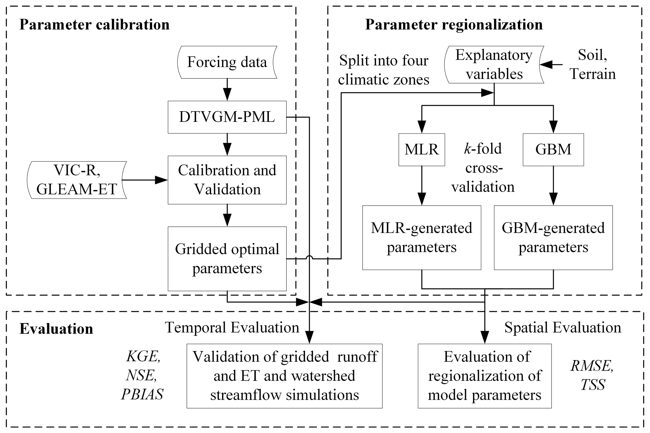
Figure 1 Flowchart of parameter calibration, validation, and regionalization. DTVGM-PML – the Distributed Time Variant Gain Model with the Penman–Monteith–Leuning equation; VIC-R – runoff simulated by the variable infiltration capacity (VIC) model; GLEAM-ET – evapotranspiration dataset from the Global Land Evaporation Amsterdam Model (GLEAM) V3.3a; MLR – stepwise multiple linear regression; GBM – gradient boost machine; KGE – Kling–Gupta efficiency; NSE – Nash–Sutcliffe efficiency; PBIAS – percent bias; RMSE – root mean square error; TSS – Taylor skill score.

2 Materials and methods

We ran a hydrological model, i.e., Distributed Time Variant Gain Model with the Penman–Monteith–Leuning equation (DTVGM-PML) developed in this study, for the country of China in a spatially distributed manner to account for within-catchment heterogeneity, the discrepancy in scale, and, thus, rainfall–runoff behavior between catchments and grid cells (Beck et al., 2020). Figure 1 presents an overview of this study. We first conducted a multivariable calibration to derive an ensemble of grid-by-grid parameter maps for regionalization. The multivariable datasets for model calibration and validation included a runoff product (Zhang et al., 2014) and an evapotranspiration (ET) dataset (Martens et al., 2017). The runoff product ($\mathrm{0.25}{}^{\circ }\times \mathrm{0.25}{}^{\circ }$) was derived from the variable infiltration capacity (VIC) model, where the simulated monthly streamflow matches well with the measurements at the major river basins in China (Zhang et al., 2014). We obtained the total runoff depths from the dataset for model calibration and validation. The ET product used in this study was the 0.25^∘ resolution Global Land Evaporation Amsterdam Model (GLEAM) V3.3a dataset (Martens et al., 2017), which has been demonstrated to estimate actual ET with reasonable accuracy in China (Yang et al., 2017).

We regionalized the model parameters using the MLR and GBM methods in terms of the explanatory variables, including topographic and edaphic characteristics. Finally, we compared the model performance with parameters from grid-by-grid calibration and regionalization.

2.1 Application of the hydrological model across China

We developed the DTVGM-PML model (Fig. 2) in this study to implement hydrological modeling across China. The original DTVGM model has been successfully applied to many river basins in China (Cai et al., 2014; Ning et al., 2016; Wang et al., 2009; Xia et al., 2005; Zeng et al., 2020; Zhan et al., 2013; Zou et al., 2017). We selected the model for its parsimonious model structure with limited free parameters due to the lack of ground-based measurements (e.g., observed streamflow) for model calibration in many regions of China. A great deal of previous studies have highlighted the importance of incorporating the vegetation change information into hydrological models to achieve better performance in hydrological simulations (Donohue et al., 2007, 2010; Gerten, 2013; Ivanov et al., 2008; Lei et al., 2014; Thompson et al., 2011). Additionally, it has been demonstrated that coupling the PML equation into hydrological models can improve the hydrological simulations under vegetation greening conditions (Bai et al., 2018a; Li et al., 2009; Zhang et al., 2009; Zhou et al., 2013). Thus, we replaced the empirical evaporation module in the DTVGM with the PML equation to improve the mechanistic representation of the ET process. We also coupled a snow routine from the HBV (Hydrologiska Byråns Vattenavdelning) model (Seibert and Vis, 2012) and the Gash rainfall interception model (van Dijk and Bruijnzeel, 2001) to improve relevant processes in DTVGM. The DTVGM-PML model ran on a grid scale, with a spatial resolution of $\mathrm{0.25}{}^{\circ }\times \mathrm{0.25}{}^{\circ }$. The gridded runoff simulated by the DTVGM-PML was routed by the Lohmann routing model for specific watersheds (Lohmann et al., 1996).

Figure 2 The model structure of the DTVGM-PML.

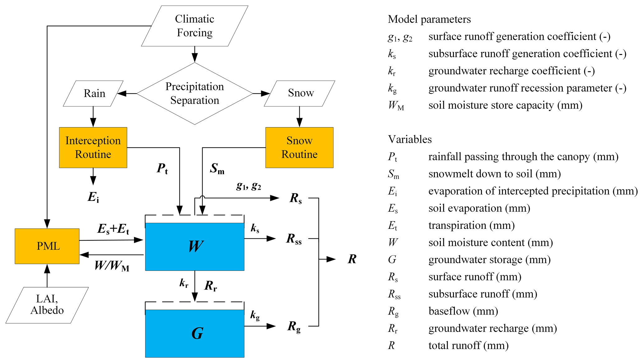
In the PML equation, we estimated the ratio of soil evaporation to the equilibrium rate (f) using the relative soil water storage, $W/W_{\mathrm{M}}$, simulated in the DTVGM. Another key parameter, the maximum stomatal conductance (g_sx), was assigned for each land cover type recommended by Zhang et al. (2017). Other insensitive parameters were held constant since ET simulations have no significant accuracy loss (Bai et al., 2018a; Leuning et al., 2008; Zhang et al., 2008).

In this study, we calibrated the following six parameters in the runoff generation process of the DTVGM-PML: two parameters (g₁, g₂) that control the nonlinear surface runoff generation, the subsurface runoff generation coefficient (k_s), the groundwater recharge coefficient (k_r) and recession coefficient (k_g), and the soil moisture storage capacity (W_M; Fig. 2). We provided detailed descriptions of the DTVGM-PML in the Supplement.

2.2 Parameter calibration strategy

In this study, we performed the 0.25^∘ grid-by-grid calibration by fitting gridded monthly runoff and ET data at a national scale (a total of 15 640 grid cells) owing to the limited long-term observed streamflow data. The modeling period spanned from 1982–2012 and consisted of 15 years (1998–2012) of the calibration period and 16 years (1982–1997) of the validation period. We used the shuffled complex evolution (SCE-UA) algorithm (Duan et al., 1992, 1994) for model calibration by minimizing a multi-variable function (see Eq. 1). The objective function is expressed as the Euclidean distance (denoted by F) that combines the Kling–Gupta efficiency (KGE; see Eq. 2; Gupta et al., 2009; Kling et al., 2012) of monthly runoff (KGE_R) and ET (KGE_ET). The KGE is a comprehensive criterion to measure the agreement between the observed and simulated values ranging from −∞ to 1, with an optimal value of 1.

$$\begin{array}{}\text{(1)}& F=\sqrt{w_{\mathrm{1}}{\left(\mathrm{1}-{\mathrm{KGE}}_{\mathrm{R}}\right)}^{\mathrm{2}}+w_{\mathrm{2}}{\left(\mathrm{1}-{\mathrm{KGE}}_{\mathrm{ET}}\right)}^{\mathrm{2}}},\end{array}$$

$$\begin{array}{}\text{(2)}& \mathrm{KGE}=\mathrm{1}-\sqrt{(r-\mathrm{1}{)}^{\mathrm{2}}+(\mathit{\beta }-\mathrm{1}{)}^{\mathrm{2}}+(\mathit{\gamma }-\mathrm{1}{)}^{\mathrm{2}}},\end{array}$$

where w₁ and w₂ are the weights assigned to runoff and ET evaluation, respectively. In this study, w₁ and w₂ were both equal to 1. r is the Pearson correlation coefficient, β denotes the bias term (i.e., a ratio of means), and γ is the variability term (i.e., a ratio of coefficients of variation).

2.3 Parameter regionalization strategy

Regionalization techniques generally include two types, such as distance-based (spatial proximity and physical similarity) and regression-based methods (He et al., 2011). In this study, we obtained the 0.25^∘ gridded parameters of the DTVGM-PML, based on a multi-variable calibration, which were then divided into four climatic zones over China (see Fig. 3; i.e., humid, semi-humid, semi-arid, and arid regions). For each grid cell, we estimated the relationship between the calibrated parameters (response variable) and physical properties (explanatory variables, e.g., topographic attributes and edaphic characteristics; see Table 1) by a machine learning technique called the gradient boosting machine (GBM; Friedman, 2001). For a comparison of the performance of GBM, we also examined a traditional regression method, i.e., the multiple linear regression method (MLR; Heuvelmans et al., 2006; Waseem et al., 2016), for parameter regionalization as the benchmark.

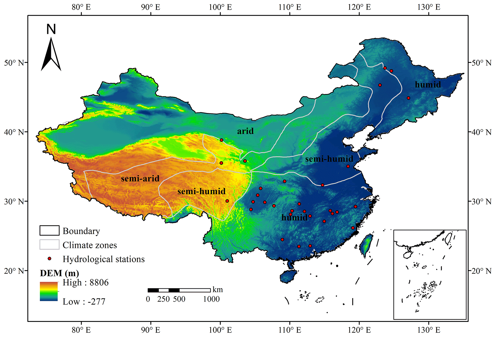
Figure 3 Location of climatic zones (humid, semi-humid, semi-arid, and arid) and hydrological stations in China.

Table 1 Model input for model simulation, training, and evaluation.

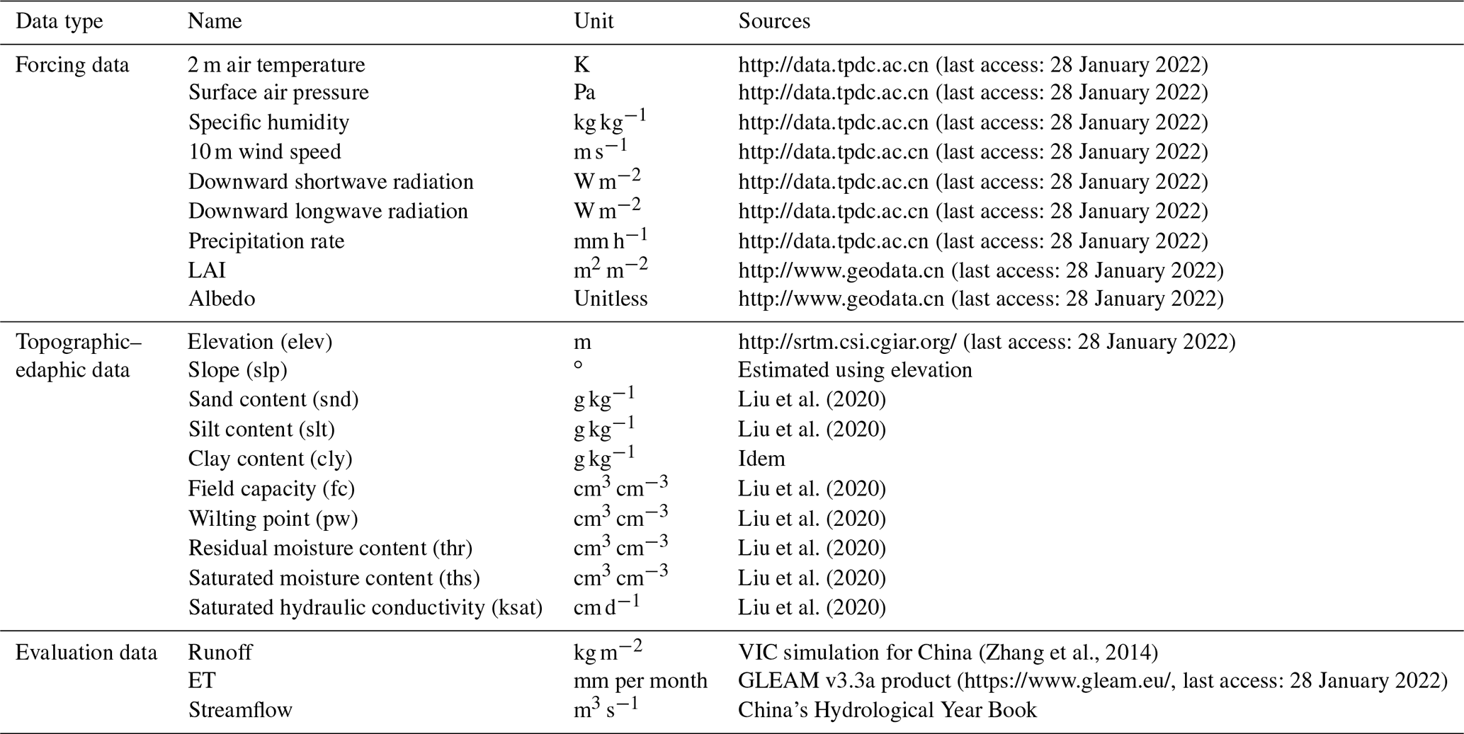
Note: the topographic–edaphic variable abbreviation is shown in the parenthesis after the variable name. LAI is the leaf area index.

The GBM is a powerful machine learning technique to train decision trees in a gradual, additive, and sequential manner (Friedman et al., 2000; Friedman, 2001; Natekin and Knoll, 2013). The main idea of the GBM is to add new models with respect to the error of the whole ensemble learned so far to the ensemble sequentially in order to boost its performance iteratively. The final GBM model is a stage-wise additive model of previous individual trees. The GBM has been proven successful across many domains, including classification problems (Lawrence, 2004; Xia et al., 2020) and regression problems (Liao et al., 2020; Xenochristou et al., 2020; Yan et al., 2019), which is the case for this study.

The MLR approach is a standard multiple linear regression to relate the response variables to the explanatory variables in a simple, fast, and straightforward manner (Lima et al., 2015; Y. Zhang et al., 2018). And the stepwise selection of predictors is applied to minimize the possible errors, resulting in the best performing model, and then identify the most influenced physiographical variable (Lima et al., 2015; Shu and Ouarda, 2012; Waseem et al., 2016). Unlike the GBM method, the MLR can explicitly quantify the relationship between explanatory variables and response variables through a regression equation.

The GBM and MLR modeling were conducted using the gbm and lmStepAIC methods, respectively, with the k-fold cross-validation in the R package of caret (Kuhn et al., 2020). The performance of the k-fold cross-validation (k=10 in this study) can help to reduce the chances of overfitting, leading to less prediction variability and, therefore, improved accuracy (Natekin and Knoll, 2013). First, we considered the following two categories of the representative explanatory variables for regression modeling in each grid cell: (i) topographic variables, e.g., elevation (meters) and slope (degrees), and (ii) edaphic variables, e.g., sand content (grams per kilogram; hereafter g kg⁻¹), silt content (g kg⁻¹), clay content (g kg⁻¹), field capacity, wilting point, residual moisture content, saturated moisture content, and saturated hydraulic conductivity (centimeters per day; hereafter cm d⁻¹). Second, we eliminated the grid cells with either KGE_R or KGE_ET less than zero, which perform poorly in simulating runoff or ET, and then split the remaining grid cells into four subsets according to the climatic zones. Finally, we trained and evaluated the GBM and MLR modeling using the model parameters in each subset and the relevant explanatory variables.

2.4 Evaluation criteria

We used the root mean square error (RMSE) to evaluate the performance of the parameter prediction based on the GBM and MLR modeling. A lower RMSE indicates a better performance than a higher one. We also calculated the Taylor skill score (TSS; Taylor, 2001) to express a synthetic measure of the prediction skill of the MLR and GBM modeling for model parameters. The TSS is a numerical summary of the Taylor diagram, varying from zero (least skillful) to one (most skillful). The TSS, as a comprehensive metric of the correlation coefficient, standard deviation, and root mean square error, has been widely used in model evaluation (Mohan and Bhaskaran, 2019; Taylor, 2001). As defined in Eq. (4), the TSS increases monotonically with increasing correlation (r→r₀) for any given variance, and increases as the modeled variance approaches the observed variance (standard deviation ratio or SDR → 1) for any given correlation. The Kling–Gupta efficiency (KGE; Gupta et al., 2009; Kling et al., 2012), percent bias (PBIAS; Gupta et al., 1999), and Nash–Sutcliffe efficiency (NSE; Nash and Sutcliffe, 1970) were used for the evaluation of model simulations based on three parameter sets. The PBIAS, varying from −∞ to +∞, measures the extent to which the simulated values are overestimated (a positive value) or underestimated (a negative value) relative to the observed values. The NSE is a widely used evaluation index to assess the predictive skill of hydrological models, which ranges from −∞ to its perfect score, that is, 1. In addition to the KGE shown in Eq. (2), other evaluation criteria are formulated as follows:

$$\begin{array}{}\text{(3)}& {\displaystyle }& {\displaystyle }\mathrm{RMSE}=\sqrt{{\displaystyle \frac{\mathrm{1}}{n}}\sum _{i=\mathrm{1}}^n{\left(X_i-Y_i\right)}^{\mathrm{2}}},\text{(4)}& {\displaystyle }& {\displaystyle }\mathrm{TSS}={\displaystyle \frac{\mathrm{4}(\mathrm{1}+r{)}^{\mathrm{4}}}{{\left(\mathrm{SDR}+\frac{\mathrm{1}}{\mathrm{SDR}}\right)}^{\mathrm{2}}{\left(\mathrm{1}+r_{\mathrm{0}}\right)}^{\mathrm{4}}}},\text{(5)}& {\displaystyle }& {\displaystyle }r={\displaystyle \frac{\frac{\mathrm{1}}{n}\sum _{i=\mathrm{1}}^n\left(X_i-\stackrel{\mathrm{‾}}{X}\right)\left(Y_i-\stackrel{\mathrm{‾}}{Y}\right)}{{\mathit{\sigma }}_X{\mathit{\sigma }}_Y}},\text{(6)}& {\displaystyle }& {\displaystyle }\mathrm{SDR}={\displaystyle \frac{{\mathit{\sigma }}_X}{{\mathit{\sigma }}_Y}},\text{(7)}& {\displaystyle }& {\displaystyle }{\mathit{\sigma }}_X=\sqrt{{\displaystyle \frac{\sum _{i=\mathrm{1}}^n{\left(X_i-\stackrel{\mathrm{‾}}{X}\right)}^{\mathrm{2}}}{n}}},{\mathit{\sigma }}_Y=\sqrt{{\displaystyle \frac{\sum _{i=\mathrm{1}}^n{\left(Y_i-\stackrel{\mathrm{‾}}{Y}\right)}^{\mathrm{2}}}{n}}},\end{array}$$

where X and Y are the calibrated parameter and regionalized parameter in DTVGM-PML (e.g., the runoff generation parameters g₁ and g₂), respectively. The subscript i denotes the ith sample of the gridded parameter. $\stackrel{\mathrm{‾}}{X}$ and $\stackrel{\mathrm{‾}}{Y}$ are the mean values of X and Y, respectively. σ_X and σ_Y are the spatial standard deviation of calibrated parameter and regionalized parameter, respectively. r represents the spatial correlation coefficient between X and Y. r₀ is the maximum correlation attainable and usually set to 0.999. SDR is the ratio of σ_X to σ_Y, and n is the total number of values for X (and Y).

$$\begin{array}{}\text{(8)}& {\displaystyle }& {\displaystyle }\mathrm{PBIAS}={\displaystyle \frac{\sum _{i=\mathrm{1}}^n\left(Y_i-X_i\right)}{\sum _{i=\mathrm{1}}^n{X}_i}}\times \mathrm{100}\mathit{\%},\text{(9)}& {\displaystyle }& {\displaystyle }\mathrm{NSE}=\mathrm{1}-{\displaystyle \frac{\sum _{i=\mathrm{1}}^n{\left(X_i-Y_i\right)}^{\mathrm{2}}}{\sum _{i=\mathrm{1}}^n{\left(X_i-\stackrel{\mathrm{‾}}{X}\right)}^{\mathrm{2}}}},\end{array}$$

where X and Y are the observed and simulated values (e.g., observed streamflow and DTVGM-PML-simulated streamflow), respectively. The subscript i denotes the ith time step (day or month) of the hydrological variables (i.e., runoff, ET, and streamflow). $\stackrel{\mathrm{‾}}{X}$ is the mean value of X, and n is the total number of values for X (and Y).

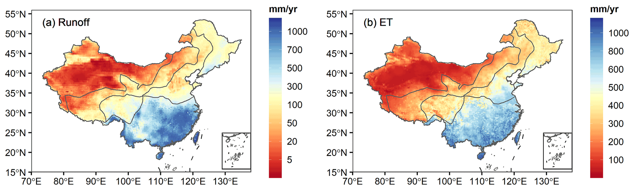
Figure 4 Spatial patterns of mean annual runoff (a) and evapotranspiration (ET) (b) simulations by the DTVGM-PML during 1982–2012.

3 Data sources and processing

Data used in this study consisted of three categories, such as forcing data, topographic–edaphic data, and evaluation data (see Table 1).

1. Model forcing data, including the climate forcing data and land surface data, were used for DTVGM-PML simulation. We used the China Meteorological Forcing Dataset (CMFD) provided by National Tibetan Plateau Data Center (He et al., 2020; Yang et al., 2010; Yang and He, 2019), which contains seven daily variables (see Table 1) with a spatial resolution of 0.1^∘. The land surface variables used here included leaf area index (LAI) and albedo obtained from the 8 d composite $\mathrm{0.05}{}^{\circ }\times \mathrm{0.05}{}^{\circ }$ GLASS product in National Earth System Science Data Center. The 8 d composite data were interpolated into the daily data, using a piecewise cubic Hermite polynomial, and then smoothed by the Savitzky–Golay filtering method (Fang et al., 2008; Li et al., 2009; Ruffin et al., 2008).

2. In total, 10 topographic–edaphic variables were considered, including topographic attributes and edaphic characteristics. The elevation and slope were derived from 90 m digital elevation model. The soil data provided by Liu et al. (2020) included eight variables summarized in Table 1 at multiple depths (0–5, 5–15, 15–30, 30–60, 60–100, and 100–200 cm). We transformed multiple-layer soil data into single-layer soil data using a weighted-average method.

3. In addition to the total runoff data from the VIC simulation for China and ET data from the GLEAM v3.3a product used for parameter calibration (Sect. 2.2), the evaluation data also included observed daily streamflow from 31 representative watersheds (see Fig. 3) for streamflow validation over China. Table S1 in the Supplement lists the basic information of the 31 hydrological stations.

Since the DTVGM-PML ran at a daily time step for 1982–2012, with a spatial resolution of 0.25^∘, all spatial data used in this study were resampled to 0.25^∘ consistently.

4 Results

4.1 Simulation of DTVGM-PML

The model calibration set out using reference data (gridded monthly runoff and ET) from the former 16 years (1982–1997) or the latter 15 years (1998–2012), with the remaining period as the validation period. The model shows slightly better results when using data from the latter period than the first period for calibration (Fig. S1 in the Supplement), which was probably due to the better data quality in the latter period than in the former period. Several previous studies have adopted this strategy, i.e., using data from the latter period for model calibration (Mizukami et al., 2017; Newman et al., 2017; Yang et al., 2018). Thus, the present study used the calibrated model parameters from the latter period for regionalization.

We also performed the comparison of model performance in hydrological simulation between the original DTVGM (without PML) and DTVGM-PML. As shown in Fig. S2, the KGE and PBIAS values of runoff simulation (Fig. S2a adn b) by DTVGM were lower than those from DTVGM-PML. The median KGE and PBIAS values of the ET simulation (Fig. S2c and d) were comparable between the two models. In summary, DTVGM-PML can help to improve hydrological simulations relative to DTVGM. Additionally, the consideration of vegetation dynamics by the PML equation in DTVGM-PML would improve the mechanistic understanding of the hydrological response under vegetation greening, which is lacking in DTVGM.

Figure 4 presents the spatial patterns of mean annual runoff and ET simulations derived from the DTVGM-PML during 1982–2012. Both the mean annual runoff and ET simulations show a decreasing trend from southeastern to northwestern China, with the highest values in humid tropical and subtropical regions, intermediate values in temperate regions, and lowest values in cold and arid regions. Figure 5 shows the model performance of runoff and ET simulations in the calibration and validation periods. The median KGE and PBIAS values for runoff simulation were 0.78 and 0.8 %, respectively, in the calibration period, and 0.69 and −14.2 %, respectively, in the validation period. The corresponding statistical values for ET simulation were 0.70 (−8.2 %) and 0.68 (−13.1 %), respectively. Overall, the DTVGM-PML could simulate the monthly runoff and ET over China well.

Figure 5 Model performance of runoff (KGE in panel a and PBIAS in panel b) and evapotranspiration (ET; KGE in panel c and PBIAS in panel d) simulations in the calibration and validation periods. The box plot was generated using data from a total of 15 640 grid cells over China. KGE denotes the Kling–Gupta efficiency. PBIAS denotes the percent bias.

4.2 Regionalization of model parameters

We evaluated the regionalization model performance in terms of RMSE for six parameters in four climatic zones. As shown in Fig. 6, GBM appears better at predicting model parameters than MLR because of the lower RMSE for all parameters in humid regions. We found consistently better accuracy of GBM in semi-humid, semi-arid, and arid areas (Figs. S3 to S5). Additionally, the difference in the model performance between GBM and MLR was significant (p value < 0.05), as per the Kruskal–Wallis test (Hollander et al., 2013). Overall, these results suggest that the performance of GBM is significantly better than that of MLR for six parameters in four climatic zones. We also calculated the Taylor skill scores (TSS) with the grid-scale calibrated parameters as the reference parameters to evaluate the regionalized model performance for estimating each parameter at each grid. As shown in Fig. S6, GBM obviously outperformed MLR with a higher TSS, suggesting that the GBM regionalized parameters presented a higher spatial agreement with reference parameter values than the MLR-generated parameters.

Figure 6 Performance evaluation of multiple linear regression (MLR) and gradient boosting machine (GBM) for six parameters, i.e., (a) g₁, (b) g₂, (c) k_s, (d) k_r, (e) k_g, and (f) W_M, in a humid region. MLR and GBM denote the multiple linear regression with stepwise selection and a gradient boosting machine model. The box plot is generated from the 10 samples in k-fold cross-validation. We use the non-parametric Kruskal–Wallis (KW) test to determine the significance of difference in the performance between MLR and GBM at a significance level of 0.05.

Figure 7 shows the spatial patterns of the three parameter sets derived from calibration and regionalization (MLR and GBM). Generally, both MLR- and GBM-derived parameters exhibited good agreement spatially with the calibrated parameters. As the model parameters were related to topography and soil properties, the parameters generated by MLR and GBM show exquisite spatial patterns and a much better spatial coherence than the calibrated parameters. Compared with the MLR-generated parameters, the GBM-generated parameters presented more consistency with the calibrated parameters in space. For example (Fig. 7e1–e3), the MLR underestimated the parameter k_g in part of Western China (nearly 0.25–0.5) relative to the calibrated parameters (about 0.5–0.8), while the GBM-derived parameters (0.5–0.75) were more consistent with calibrated values. In summary, the regionalized parameters generated by the regionalization methods (MLR and GBM) exhibited better spatial coherence relative to the calibrated parameters with spatial discontinuities. The GBM derived more accordant parameters with the calibration than the MLR.

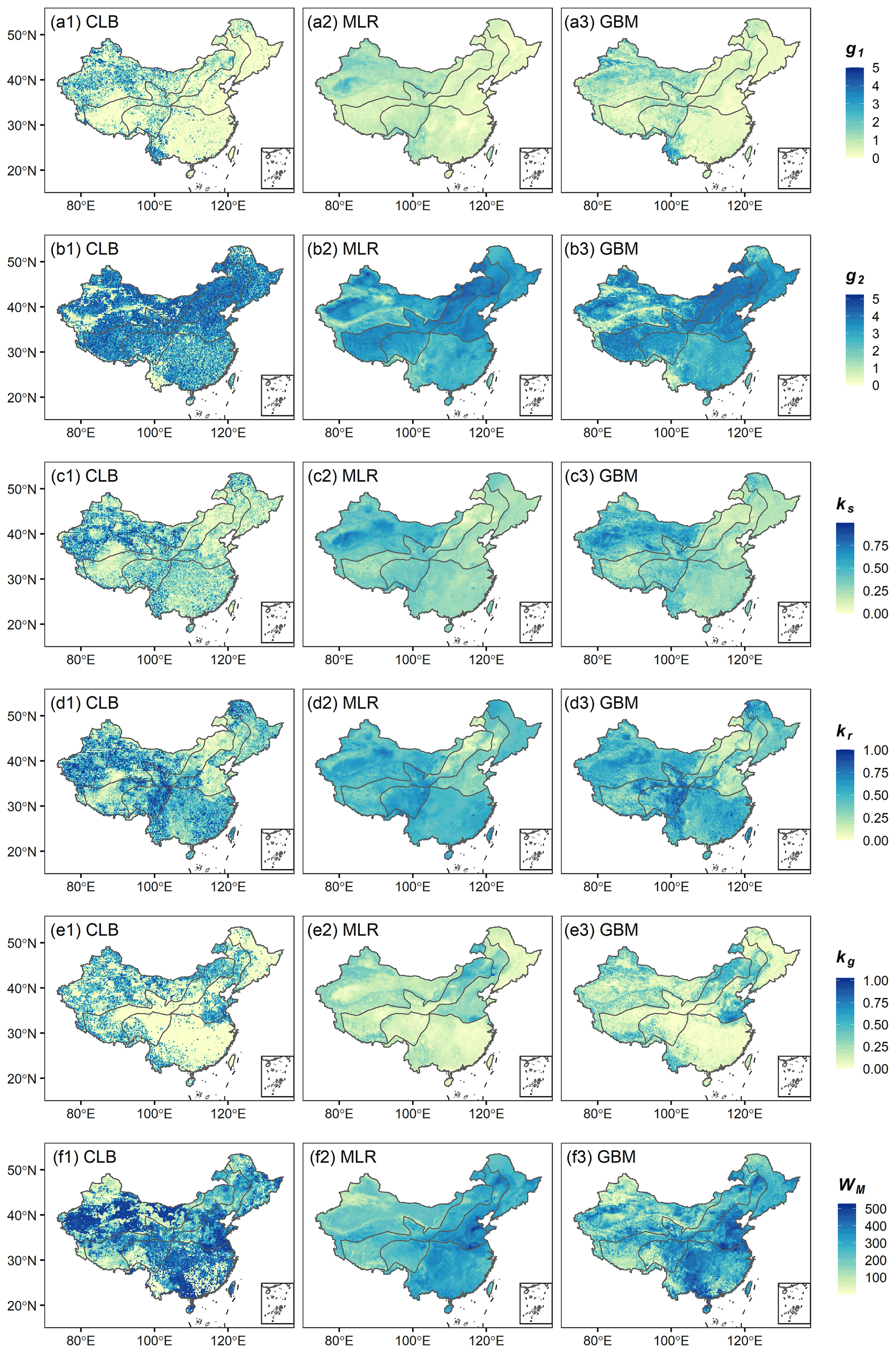
Figure 7 Spatial patterns of the model parameters, i.e., (a) g₁, (b) g₂, (c) k_s, (d) k_r, (e) k_g, and (f) W_M, derived from (1) calibration (CLB), (2) multiple linear regression (MLR), and the (3) gradient boosting machine (GBM).

4.3 Validation of gridded runoff and ET simulations based on parameter regionalization

To assess the effectiveness of parameter regionalization, we compared the model performance of the runoff and ET simulations with the regionalized parameter sets (MLR and GBM) to that with the calibrated parameters. Figure 8 presents cumulative density function (CDF) plots of KGE values for runoff simulations in both the calibration (solid lines) and validation (dashed lines) periods over four climatic zones. The KGE values were computed based on the DTVGM-PML simulations using the following three parameter sets: (1) grid-by-grid calibration (black lines), (2) MLR generation (blue lines), and (3) GBM generation (red lines).

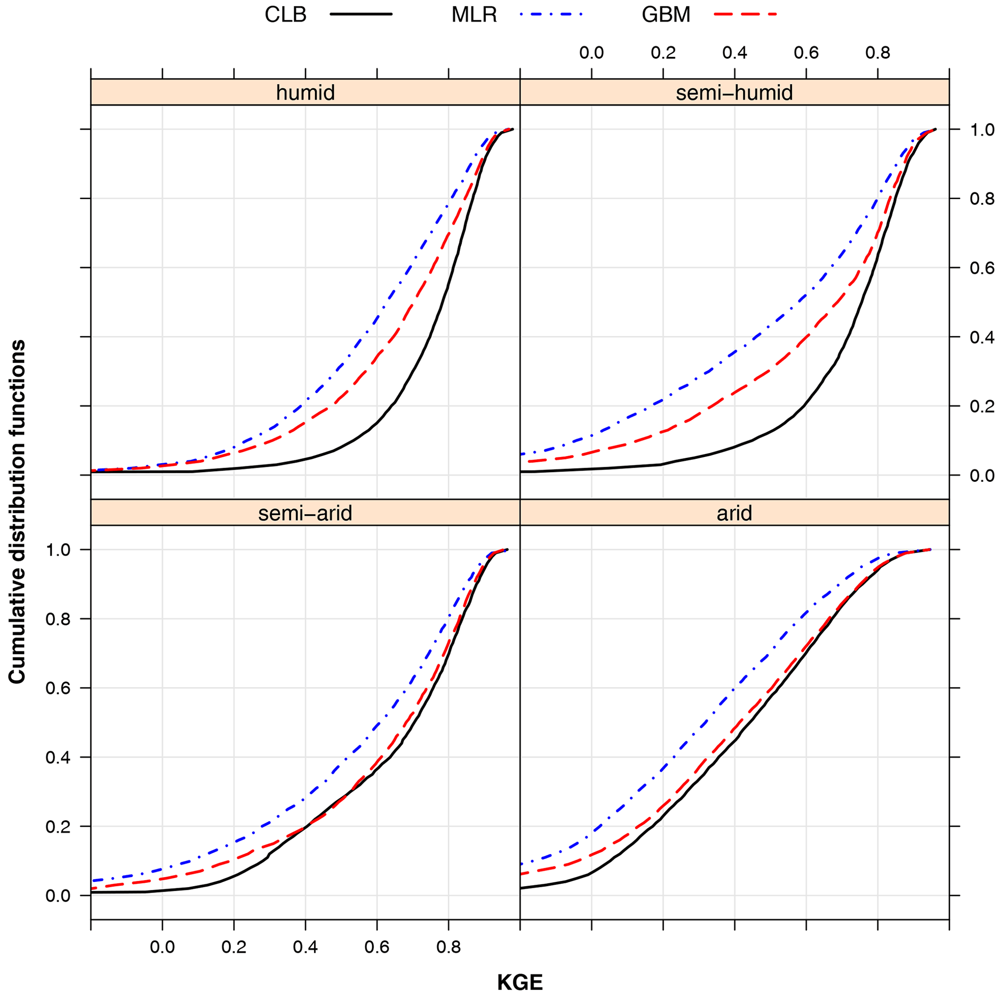
Figure 8 Cumulative density functions (CDFs) of KGE for runoff simulation based on three parameter sets – black lines are for calibration (CLB), blue lines are for multiple linear regression (MLR), and red lines are for the gradient boosting machine (GBM) – in the validation period over four climatic zones. KGE denotes the Kling–Gupta efficiency.

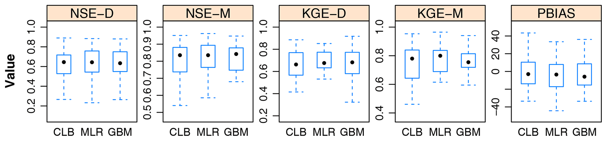
Figure 9 The model performance statistics of streamflow simulations on 31 hydrological stations based on three parameter sets. “D” and “M” denote the daily and monthly evaluations, respectively.

Regarding the runoff simulation (Fig. 8), median KGE values produced by calibrated parameters were 0.783 in humid regions, 0.755 in semi-humid regions, 0.704 in semi-arid regions, and 0.442 in arid regions for the validation period. The median KGE score based on the MLR method was worse by 0.139 averaged in four climatic zones than that from simulation using calibrated parameters for the validation period. While, as shown in Fig. 8, all the KGE values in the four regions from GBM parameters were superior to the MLR parameters. The corresponding difference of KGE was 0.023 relative to the calibration for the validation period.

In contrast to runoff simulation, however, the distributions of KGE for the ET simulation from the regionalized parameters were significantly close to those based on the calibrated parameters in each region, as shown in Fig. S7. The median KGE values from three parameter sets were around 0.68 in humid regions, 0.74 in semi-humid regions, 0.72 in semi-arid regions, and 0.53 in arid regions for the validation period. Overall, the performance of the ET simulation from regionalization was satisfactorily comparable to that from calibration.

4.4 Validation of watershed streamflow simulations based on parameter regionalization

To give insight into the performance of streamflow simulations based on parameter regionalization, we calculated NSE, KGE, and PBIAS at 31 representative watersheds with both daily and monthly streamflow validation (Fig. 9). According to the Kruskal–Wallis test, there were insignificant differences (p values > 0.05) in five criteria based on the three parameter sets. Both MLR and GBM performed as well as the calibration, with high median scores of NSE and KGE at both daily (NSE was nearly 0.64 and KGE was nearly 0.67) and monthly (NSE was nearly 0.84 and KGE was nearly 0.78) scales and median PBIAS close to zero (around −4.1 %). Since the stations were almost located in humid and semi-humid regions (28 of 31 in Fig. 3), we could expect that the parameters derived from the regionalization can reasonably generate monthly streamflow with good agreement to the observations (in line with results from Fig. 8). We also obtained encouraging results from the daily streamflow simulation with satisfying accuracy. In terms of the three stations in the arid and semi-arid regions, the performance of MLR was slightly poorer than that of calibration and GBM, as the daily and monthly NSE values, for instance, at Tangnaihai station, were 0.494 and 0.586 compared with the corresponding values of 0.675 and 0.751 for calibration and 0.631 and 0.719 for GBM, respectively.

4.5 Identification of important factors for model parameters

We further estimated the relative importance of each explanatory variable based on the GBM model, which was determined by averaging the improvement (decrease) in the squared error at each split over all the trees made by each variable, with a range from 0 (least important) and 100 (most important; Natekin and Knoll, 2013; Xia et al., 2020). Figure 10 presents the relative importance of the explanatory variables from the GBM model for all six parameters in four climatic zones and the margin plots containing the mean relative importance for each parameter or each climatic zone.

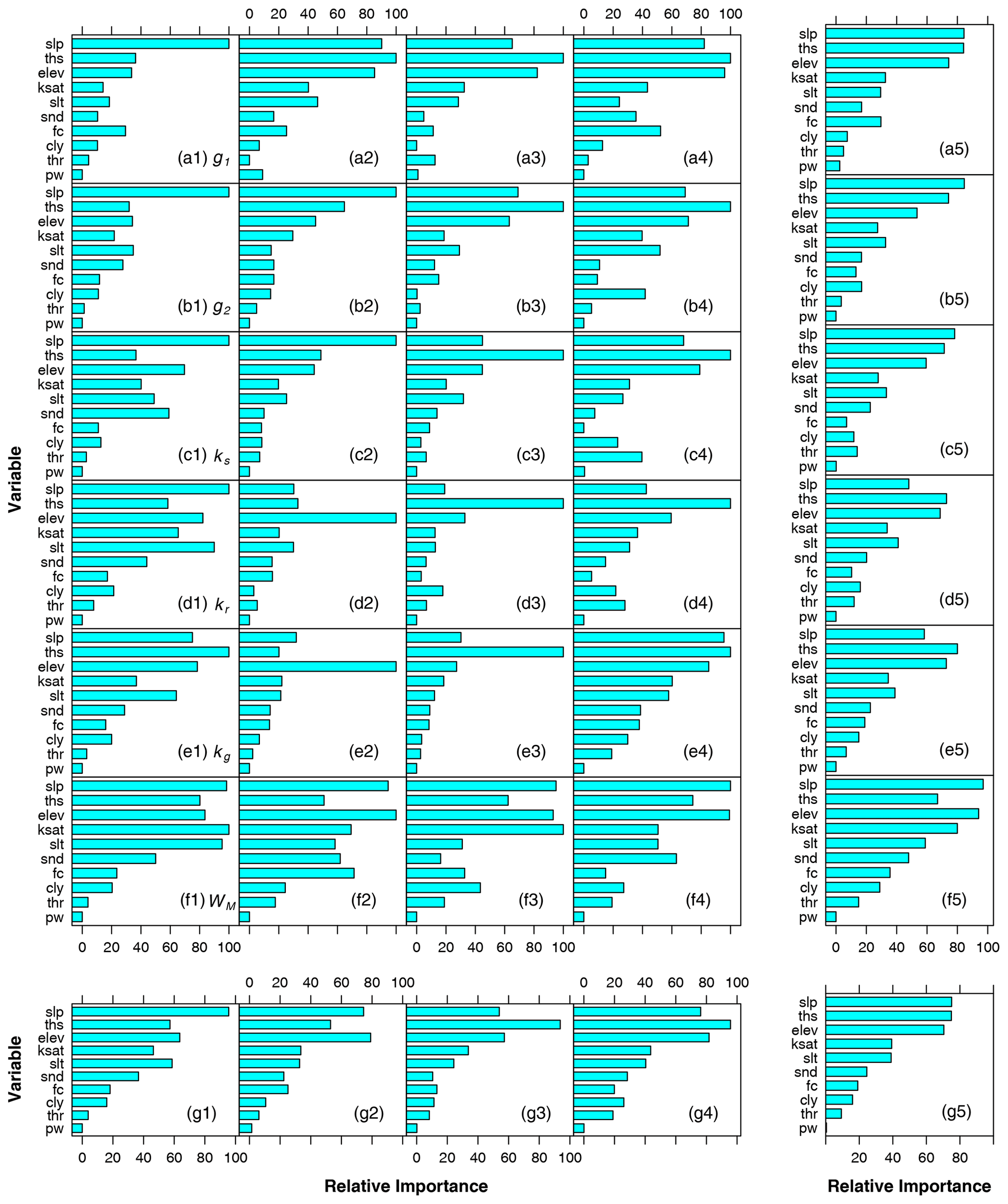
Figure 10 Relative importance of explanatory variables from the gradient boosting machine (GBM) model for (a) g₁, (b) g₂, (c) k_s, (d) k_r, (e) k_g, and (f) W_M in four climatic zones (1 – humid; 2 – semi-humid; 3 – semi-arid; 4 – arid). The mean relative importance over the four regions for each parameter is shown in the right column (a5–g5). The mean relative importance over six parameters for each climatic zone is shown in the bottom row (g1–g5). Explanatory variables include elev (elevation), slp (slope), snd (sand content), slt (silt content), cly (clay content), fc (field capacity), pw (wilting point), thr (residual moisture content), ths (saturated moisture content), and ksat (saturated hydraulic conductivity).

Generally, we found that the slope (slp), saturated moisture content (ths), and elevation (elev) were the most critical explanatory variables to inform the model parameters (Fig. 10g5), whereas there were several differences among parameters or regions. In humid and semi-humid regions, the terrain properties, including slope and elevation, were likely to determine most model parameters (Fig. 10g1 and g2). As for semi-arid and arid regions, most parameters primarily depended on the saturated moisture content that becomes a constraining factor for runoff generation in dry areas. For the three parameters (g₁, g₂, and k_s) that control surface and subsurface runoff generation, the dominant factors were slope and saturated moisture content (Fig. 10a5, b5, and c5). However, the parameters for groundwater recharge (k_r) and recession (k_g) were mainly controlled by the saturated moisture content, followed by elevation (Fig. 10d5 and e5). In terms of the parameter W_M, which represents the soil moisture storage capacity, i.e., the slope, elevation followed by the saturated hydraulic conductivity were more essential predictors than the saturated moisture content (Fig. 10f5).

5 Discussion

5.1 Performance of calibration and regionalization for DTVGM-PML

Previous studies have established the effectiveness of the multivariate calibration framework for hydrological models (Bai et al., 2018b; Dembélé et al., 2020; Demirel et al., 2018; Finger et al., 2015; Nijzink et al., 2018; Xie et al., 2020). The current study performed a multiple variable calibration strategy to calibrate model parameters in each grid against the reference datasets (VIC runoff and GLEAM ET) during the 15-year calibration period, followed by an independent model validation against the reference gridded runoff and ET during the 16-year validation period. We also validated the model using observed streamflow at 31 representative hydrological stations in diverse climatic zones. The gridded runoff in each watershed was routed to the corresponding hydrological station using consistent routing parameters. Despite the fact that the streamflow data are commonly used in the calibration of hydrological models (Dembélé et al., 2020), previous studies have explored the potential in model calibration solely against remotely sensed ET data (without the need for gauged streamflow data) and achieved encouraging results in streamflow simulation (Huang et al., 2020; Zhang et al., 2020). The satisfactory performance in the model validation of streamflow suggests the high reliability of the multivariate calibration strategy used in this study.

Hydrological simulation in arid and semi-arid regions is still challenging (Huang et al., 2016; Wheater et al., 2007; Yang et al., 2019). There appears to be a better performance in runoff simulations in (semi-)humid regions than (semi-)arid regions (Fig. 8). Regionalization methods tend to perform more poorly in drier regions, which is expected in common modeling practices (Guo et al., 2021; Parajka et al., 2013a). The results support the general knowledge of runoff prediction in different climatic zones, i.e., it is more challenging to achieve good performance in (semi-)arid regions than humid regions. The relatively poor performance in (semi-)arid regions may be attributed to model structural deficiencies, forcing errors, and uncertainties in the reference data for calibration. For example, the large-scale hydrological models may ignore complex processes like surface–groundwater interactions and channel losses (Oubeidillah et al., 2014). The quality of the forcing data (e.g., precipitation) also influences the performance of hydrological models in runoff simulation (Mizukami et al., 2017). Wang et al. (2016) found systematic overestimates of CMFD precipitation over the Qinghai–Tibetan Plateau. Furthermore, unlike the observed streamflow, the reference data, such as runoff and ET data, are not the standard actual observed data. This might also explain the better performance in our model validation against observed streamflow at the watershed scale with regionalized parameters than calibrated parameters. Zhang et al. (2014) suggested that the data should be used with caution in Western China as there are significant potential uncertainties in the hydrologic simulation due to the lack of meteorological observations. And issues in arid regions have always been a challenge for the VIC model (Oubeidillah et al., 2014; Yang et al., 2019). Yang et al. (2017) indicated that the GLEAM ET data showed a significant systematic bias and overestimated the eddy covariance ET measurements at forest sites. We argue that these reanalysis datasets are precious for the large-scale calibration of hydrological models in terms of both spatial and temporal dynamics, though they will inevitably introduce uncertainties to a certain degree.

5.2 Prediction of model parameters by machine learning methods

Given the complex and nonlinear relationships with high nonstationarity between physical catchment descriptors and model parameters, it is a daunting challenge to develop a robust method for the regionalization of hydrological models (Guo et al., 2021). Machine learning approaches provide a promising tool, as an alternative to conventional linear regression models, to regionalize hydrological model parameters. Machine learning techniques are focused on specific tasks, like classification and regression, and have been widely used for many hydrological issues (Adnan et al., 2019; Huntingford et al., 2019; Lima et al., 2015; Rajaee et al., 2019; Shen, 2018; Yaseen et al., 2015; Z. Zhang et al., 2018). In this study, we built a predictive GBM model for the parameter regionalization of DTVGM-PML compared with an MLR model using the terrain and soil properties as explanatory variables. Overall, the GBM outperformed the MLR based on evaluation in the following three aspects: (i) higher accuracy in reproducing the calibrated parameters, as indicated by significantly lower RMSE with GBM against MLR (Fig. 6), and more consistent spatial patterns with calibrated parameter values (Fig. 7), (ii) better performance in runoff simulations based on parameters generated from GBM than MLR (Fig. 8), and (iii) comparable results of streamflow validation in 31 watersheds based on regionalization and better performance in several stations in (semi-)arid regions by GBM than MLR (Fig. 9). Note that the parameters in the ET estimation (PML method in DTVGM-PML) were not involved in model calibration. Consequently, the performance of ET simulation from regionalization was comparable to that from calibration (Fig. S7). Taken together, the GBM method, as an ensemble technique, can achieve higher accuracy in parameter regionalization than MLR (Natekin and Knoll, 2013).

We noticed that the GBM outperformed the MLR in grid-scale runoff simulations but showed an insignificant difference in watershed streamflow validation. It is likely because of the following reasons: (i) the observed watershed streamflow data are independent of the gridded runoff data in this study, which could lead to differential modeling performance in these two datasets; (ii) most of the watersheds (i.e., 28 out of 31) for streamflow validation are within humid regions, where the difference in performance of grid-scale runoff simulations was relatively small, when compared with non-humid regions, between regionalized and calibrated parameters; and (iii) the flow routing of the grid-scale runoff within a watershed may smooth the heterogeneity in runoff from multiple spatially distributed grids. We suggest that streamflow from diverse watersheds, especially in arid regions, is needed for model validation with parameters derived from different regionalization approaches. The possible inconsistencies in the results between the evaluation of the parameter regionalization and the validation of streamflow also imply the necessity of watershed-scale streamflow validation following parameter regionalization.

The proposed GBM method explored the relationship between model parameters and the terrain and soil attributes and offered a helpful approach to estimate model parameters for hydrological simulations. It can also achieve satisfactory accuracy, especially in (semi-)humid regions. This study also motivates further investigations including, but not limited to (i) improvement in the model structure to better represent hydrological mechanisms in complicated underlying surface conditions and changing environment and the (ii) selection of more physical attributes, such as vegetation or climatic factors, for regionalization.

Although the GBM cannot provide an explicit formula that intuitively links the response variable with explanatory variables like the MLR, it can estimate response variables based on explanatory variables. More importantly, the machine-learning-based regionalization methods can identify essential driving factors which develop a primary appraisal of how important terrain and soil properties are for parameters of hydrological models.

5.3 Important attributes dominating model parameters

The runoff process is primarily controlled by regional climatic regime, vegetation, land use, topography, and soils (Dunne and Leopold, 1978; Freeze, 1974; Mizukami et al., 2017; Tarboton, 2003). We used the GBM method to predict parameter values from available topographic and edaphic properties, such as slope, elevation, saturated moisture content, saturated hydraulic conductivity, field capacity, and soil texture. Our findings of the variable importance when using the GBM model quantitatively indicate that the runoff generation parameters of DTVGM-PML are majorly controlled by slope, saturated moisture content, and elevation. Moreover, the results in different climatic zones show that terrain attributes significantly influence the runoff process in relatively humid regions. At the same time, the saturated moisture content becomes a limiting factor in drier areas.

Prior studies have noted the incredible impact of slope on runoff generation (Akbarimehr and Naghdi, 2012; Chaplot and Le Bissonnais, 2003; Garg et al., 2013; Tarboton, 2003). Steeper slopes lead to faster drainage in aquifers (Beck et al., 2020; Post and Jakeman, 1996; Zecharias and Brutsaert, 1988). The slope seems to be the most critical factor for parameters g₁, g₂, and k_s that control surface and subsurface runoff generation. Garg et al. (2013) investigated how the slope affects surface runoff estimation significantly for the Solani watershed in northern India using the modified NRCS-CN (Natural Resources Conservation Service curve number) method. Several reports have shown that storm runoff by subsurface flow requires steep, convex slopes and high saturated hydraulic conductivities (Freeze, 1972, 1974; Montgomery and Dietrich, 2002). The parameter g₁ presents the surface runoff coefficient when the soil water storage reaches its maximum value, i.e., $W/W_{\mathrm{M}}=\mathrm{1}$, and the parameter g₂ is the power of the relative soil water storage ($W/W_{\mathrm{M}}$). A steeper slope results in an increase in the value of g₁ and a decrease in g₂ (Fig. S8a1 and b1), thus leading to an increase in the amount of surface runoff, which supports the previous findings that runoff amount increases with increasing slope (Chaplot and Le Bissonnais, 2003; Huang, 1995).

Regarding the groundwater recharge and baseflow, the corresponding parameters (k_r and k_s) strongly depend on the saturated moisture content. The results are consistent with Chiew and Siriwardena (2005), who found that the groundwater recharge parameter and baseflow recession parameter of the SIMHYD model (a simplified version of the HYDROLOG model) are highly correlated with the plant-available water holding capacity, a proxy of the soil water storage capacity (Mckenzie et al., 2000). While concerning the soil moisture storage capacity, W_M, in DTVGM-PML, the saturated moisture content is likely to be less important than the slope, elevation, and saturated hydrologic conductivity. Note that W_M is different from the saturated moisture content in soil. The latter is equivalent to the effective porosity and is simplified as a one-layer value in this study, whereas the soil moisture state variables in many conceptual hydrological models do not act in the same way as in the real world (Zhuo and Han, 2016). The surface slope is correlated with soil depth (Tesfa et al., 2009), which strongly influences W_M. If the soil depth data, more likely to be associated with W_M, are available, then they should be incorporated in parameter regionalization to obtain more reliable and intelligible results.

5.4 Necessity of parameter regionalization

Hydrologic models often rely on regionalization approaches to transfer information from small to large spatial scales (e.g., from grid cell to subbasin, watershed, and regional scale; Beck et al., 2020; Mizukami et al., 2017) and from gauged to ungauged catchments (He et al., 2011; Hrachowitz et al., 2013; Pagliero et al., 2019; Parajka et al., 2013b). In this study, though parameters were calibrated and, thus, available at each grid cell, the parameter values at around 450 grid cells were not reliable owning to poor model performance (i.e., KGE < 0; Knoben et al., 2018; Koskinen et al., 2017; Sutanudjaja et al., 2018). Therefore, we only used the calibrated parameters with KGE ≥ 0 (i.e., representing better model performance) for the regionalization of parameters. The model performance for 53 % of these grid cells (with KGE < 0 prior to regionalization) were improved when we reran the model with regionalized parameters. Particularly, the KGE values in 37 % of the grid cells (with KGE < 0 prior to regionalization) became positive, indicating a substantial improvement in the modeling performance.

Even though the parameters were well calibrated and available at each grid cell, one might consider whether and which topographic and edaphic properties mediate these hydrological parameters. Our machine-learning-based (i.e., GBM) regionalization of parameters enables us to estimate six key hydrological parameters using site-specific characteristics. Following the regionalization of the parameters, our results of variable importance quantitatively indicate that the runoff generation parameters are majorly controlled by slope, saturated soil moisture content, and elevation. Moreover, the terrain attributes significantly regulate the runoff processes in relatively humid regions, while the saturated soil moisture content becomes a limiting factor in arid areas. The regionalization of parameters will improve our mechanistic understanding of the runoff generation processes and associated key hydrological parameters under different topographic and edaphic conditions.

6 Conclusion

We conducted parameter regionalization for the DTVGM-PML model using a machine learning technique, i.e., the gradient boosting machine, compared with the traditional multiple linear regression method. We show that the GBM model is superior to the MLR in predicting model parameters as a function of topographic and edaphic characteristics due to its significantly lower biases and higher spatial agreement for almost all parameters in four distinct climatic zones. The regionalized parameters also exhibited better spatial coherence relative to the grid-by-grid calibrated parameters. Regarding the model validation of streamflow simulations in 31 hydrological stations, MLR- and GBM-generated parameters could simulate streamflow as accurately as the results with grid-by-grid calibrated parameters (the median daily and monthly NSE are 0.65 and 0.84, respectively), with the GBM being preferable to MLR in the arid regions. This study suggests that the watershed-scale streamflow validation following parameter regionalization is necessary due to potentially inconsistent results between the parameter regionalization evaluation and the streamflow validation. Based on the GBM regionalization results, we found that the slope, saturated moisture content, and elevation are the most important explanatory variables to inform model parameters. Our results indicate that machine learning techniques can be a useful alternative to the conventional regression approach to better predict hydrological model parameters. This is particularly significant for hydrological predictions in ungauged basins. The methods developed and insights gained from this study can also improve the interpretation and prediction of parameters in other large-scale hydrological and environmental models.