the Creative Commons Attribution 4.0 License.
the Creative Commons Attribution 4.0 License.
 | 28 Sep 2022
Leveraging sap flow data in a catchment-scale hybrid model to improve soil moisture and transpiration estimates
Maoya Bassiouni
Anke Hildebrandt
Sibylle K. Hassler
Erwin Zehe
Sap flow encodes information about how plants regulate the opening and closing of stomata in response to varying soil water supply and atmospheric water demand. This study leverages this valuable information with model–data integration and deep learning to estimate canopy conductance in a hybrid catchment-scale model for more accurate hydrological simulations. Using data from three consecutive growing seasons, we first highlight that integrating canopy conductance inferred from sap flow data in a hydrological model leads to more realistic soil moisture estimates than using the conventional Jarvis–Stewart equation, particularly during drought conditions. The applicability of this first approach is, however, limited to the period where sap flow data are available. To overcome this limitation, we subsequently train a recurrent neural network (RNN) to predict catchment-averaged sap velocities based on standard hourly meteorological data. These simulated velocities are then used to estimate canopy conductance, allowing simulations for periods without sap flow data. We show that the hybrid model, which uses the canopy conductance from the machine learning (ML) approach, matches soil moisture and transpiration equally as well as model runs using observed sap flow data and has good potential for extrapolation beyond the study site. We conclude that such hybrid approaches open promising avenues for parametrizations of complex water–plant dynamics by improving our ability to incorporate novel or untypical data sets into hydrological models.
- Article
(4690 KB) - Full-text XML
- BibTeX
- EndNote


Globally, about 26 % to 40 % of the precipitation that falls on the continents is transpired by vegetation, making it one of the dominant fluxes of the terrestrial water cycle (Dingman, 2015). Seasonal variations in plant–water use can thus significantly affect the water balance of catchments, modify its runoff generation, and change its dynamic water storage (Brown et al., 2005; Hrachowitz et al., 2021; Seibert et al., 2017). Understanding the role of ecosystems in catchment hydrology is crucial, particularly when investigating the impacts of climate change (e.g., Duethmann et al., 2020). Estimating transpiration at the catchment scale is, however, challenging since plant–water uptake is difficult to measure, parameterize, and scale up from the individual plant to the ecosystem level (e.g., Mencuccini et al., 2019). As a consequence, the predictive performance of hydrological models, which represent water balance and vegetation dynamics in a physically consisted manner, can be limited due to the a priori chosen vegetation-process parameterizations and parameter values (e.g., Bennett and Nijssen, 2021; Gharari et al., 2021; Mendoza et al., 2015). Improving these uncertain parameterizations requires methods that can combine process-based hydrological models with new information about how plant transpiration varies with environmental conditions.
Flux towers provide the state-of-the-art evapotranspiration data to train and validate hydrological models. One caveat in using these measurements is that they represent an effective flux integrating evaporation from the canopy interception store and the soil with plant transpiration. An accurate partitioning of this integral flux into its components is, however, of key importance for improving transpiration modeling under changing conditions (Stoy et al., 2019), including effects of land-use changes such as deforestation (e.g., Hrachowitz et al., 2021) and forest regeneration (e.g., Neill et al., 2021). This is a key reason why sap flow is used as independent measurement technique to characterize transpiration dynamics in forest (e.g., Granier and Loustau, 1994) and agricultural ecosystems (e.g., Dugas et al., 1994). While originally established in the plant physiology community, sap flow data have also proven useful in hydrological research. For instance, Renner et al. (2016) showed that stand composition of forests can counteract differences in sap flow on south- and north-facing slopes, leading to similar transpiration rates on both expositions. Hoek van Dijke et al. (2019) found that the normalized difference vegetation index (NDVI) successfully captured sap flow dynamics during the green-up phase, although it failed under dry conditions. Hassler et al. (2018) highlighted that spatial differences of atmospheric demands and soil moisture only explain a small fraction of observed spatial variation of sap flow, while site-specific factors, like geology and aspect, were more important. These findings imply that accounting for relations between vegetation characteristics, hydrometeorological drivers, and catchment properties can improve transpiration estimates and exemplifies the potential of using sap flow data to advance hydrological simulations. The value of sap flow information is emphasized by the growing availability of global open-source sap flow databases (Poyatos et al., 2016) that provide opportunities to develop generalized relations to better inform hydrological models at places where no sap flow data are available.
Plants adapt transpiration depending on atmospheric water demand and supply. One important regulation mechanism is the opening and closing of the pores on their leaves, called stomata, to regulate their CO2 and water vapor exchange with the atmosphere. This process crucially governs the transpiration of plants, which is also reflected by the wide range of stomatal conductance models that are available in hydrological models (e.g., Damour et al., 2010). One issue is that these stomatal conductance models typically rely on several site-specific parameters, and each approach has its own limitations which makes the choice of the “right” process parameterization challenging. In this context, it is interesting to note that sap flow can, besides being used to estimate transpiration directly, also be used to infer canopy conductance or stomatal conductance scaled by leaf area index (LAI). This is done by inverting a simplified formulation of either Fick's Law or the Penman–Monteith equation (e.g., Ewers and Oren, 2000; Köstner et al., 1992; Phillips and Oren, 1998).
While the complex interactions between soil water supply, vegetation behavior, and meteorology are challenging to parameterize in bottom-up empirical or physically based stomatal conductance models, machine learning (ML) methods have recently proven to be a particularly useful alternative to reproduce ecohydrological behavior and estimate transpiration (e.g., Fan et al., 2021; Zheng et al., 2021). However, despite their recent success, ML approaches also have shortcomings as they do not ensure mass and energy conservation and lack physical constraints. The latter makes extrapolation and simulation under changing boundary conditions challenging. Hybrid models that combine physical knowledge of process equations with the flexibility of data-driven predictions are therefore a promising tool to estimate fluxes and state variables in the Earth's system (e.g., Reichstein et al., 2019).
In this study, we propose and test a hybrid ML approach to integrate sap flow data into a process-based hydrological model, and explore opportunities for improving soil moisture and transpiration estimates at the catchment scale. Specifically, we leverage an extensive sap flow data set, spanning a drought period, in a subcatchment of the well-monitored and well-studied Attert experimental observatory (Pfister et al., 2002). We first integrate canopy conductance inferred from sap flow data into a process-based hydrological model and compare its performance to the benchmark model that uses an empirical stomatal conductance equation. We then train a recurrent neural network (RNN) based on standard hourly meteorological data, to predict sap flow beyond the temporal extent of the training period. These simulated velocities are then used to estimate canopy conductance, allowing us to replace the empirical stomatal conductance equation in the hydrological model on forward simulations beyond the monitoring periods. Our results support the value of such hybrid-model approaches by comparing the different model variants against each other and against hydrological data, such as soil moisture and discharge. Importantly, we highlight the value of sap flow measurement campaigns for improving simulation at the catchment scale.
2.1 Study area
The Weierbach is a 0.44 km2 large experimental headwater catchment, nested in the Colpach catchment and located in Luxembourg (Fig. 1; Hissler et al., 2021). The catchment is characterized by coarse-grained and highly permeable soils and a slate bedrock (Ardennes massif). It has a temperate semi-marine climate with a mean annual rainfall of 950 mm and mean monthly temperatures that range between 0 ∘C in January and 17 ∘C in July. Precipitation is evenly distributed across the seasons while the runoff generation has a distinct seasonal pattern with around 80 % of the annual discharge being released between October and March (Loritz et al., 2021). The Weierbach catchment is entirely forested and dominated (>70 %) by deciduous beech trees (Fagus sylvatica) and oak trees (Quercus spec). A detailed description of the Weierbach catchment and a comprehensive open-access hydrological data set can be found in Hissler et al. (2021). The Colpach is the parenting catchment of the Weierbach, located in the same hydropedological area and characterized by a similar runoff generation and formation (Loritz et al. 2019), but it comprises a larger variety of land-cover types (65 % forest, 35 % agriculture).
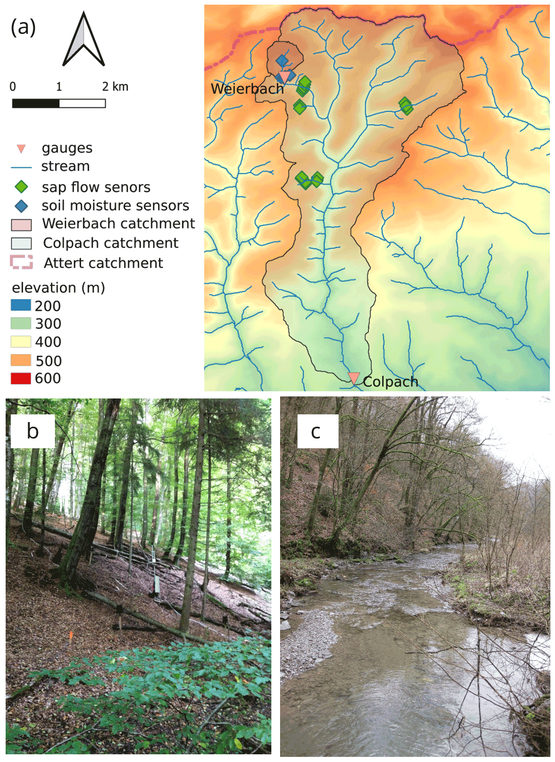
Figure 1(a) Map of the Colpach and Weierbach catchments (location: northern Luxembourg) indicating the gauges, soil moisture, and sap flow sensors. Panel (b) is a picture of a typical forested hillslope within the Colpach catchment with installed sap flow sensors, and (c) shows the Colpach River around 4 km north of the gauging station.
2.1.1 Hydrometeorological data
This study requires hourly meteorological data to force the water balance simulations and to calculate canopy conductance. For all these purposes, we use data records from April 2014 to October 2016. We obtain air temperature (∘C), relative humidity (%) and rainfall data (mm h−1) from the Holtz meteorological station available in the open-access data set from Hissler et al. (2021). We obtain measurements of wind speed (m s−1) and global radiation (W m2) from a meteorological station around 500 m southeast of the catchment available from the Catchment as Organized Systems (CaOS) project observation network (Zehe et al., 2014). Additionally, we use discharge data and averaged soil moisture from Hissler et al. (2021) at 10 and 60 cm depth (based on six individual sensors in each depth) to quantify the performance of hydrological model simulations. Soil moisture was additionally corrected for a stone content of 10 % and 30 % in 10 and 60 cm based on several soil profiles in the research area (Jackisch, 2015).
2.1.2 Sap velocity measurements
We use hourly sap velocities (cm h−1), the rate of water flow through a tree, from three growing seasons (April–October; 2014–2016) of an extensive measurement campaign in the Colpach catchment (detailed description in Hassler et al., 2018). We use a subset of the original data set of Hassler et al. (2018) comprising 32 trees, including 17 beech trees (Fagus sylvatica), 11 oaks (Quercus spec.), 2 hornbeams (Carpinus betulus) and 2 common alders (Alnus glutinosa) with individual tree diameters at breast height ranging from 8 to 80 cm (average 32 cm). Sample distribution ranges from north- to south-facing slopes and up- and downslope sectors, specifically selected to capture the typical hydropedological characteristics of the Colpach and the Weierbach catchments. Before the growing season, the campaign equipped each tree with sap flow sensors, manufactured by East 30 Sensors (Washington, USA). The sensors have three measurement depths, i.e., at 5, 18, and 30 mm in the xylem and measure sap velocity with the heat ratio method (Campbell et al., 1991; Burgess et al., 2001; Hassler et al., 2018). We estimate tree-specific sap velocities by calculating the median from the measurements at the three different xylem depths. We use the median to account for the skewed distribution of sap velocities inside the sap wood, as sap velocities typically decrease closer to the heartwood (e.g., Gebauer et al., 2008; Jackisch et al., 2020).
2.1.3 Catchment-level transpiration based on sap flow
This study focuses on catchment-level transpiration to circumvent the challenge and uncertainty of characterizing transpiration from individual tree sap flow (e.g., Gebauer et al., 2008; Zhang et al., 2015) and to remain scale consistent with simulated transpiration of the hydrological model. We employ an integral approach, assuming that the tree sample is representative for the age spectrum in the catchment and that trees dominate transpiration in this forested catchment compared to understory and herbaceous vegetation. We average the 32 tree-specific sap velocities to obtain a time series representing an average tree in the study area. We then obtain average hourly catchment-level transpiration per unit ground area (Tsap, m s−1) based on sap flow by multiplying the catchment-averaged sap velocity by the catchment-averaged tree density of 42 m2 ha−1 (Hassler et al., 2018). This calculation assumes that water storage in the tree relative to the transpiration flux is negligible. Therefore, the observed daytime water flux through the tree is equal to the transpiration flux through the leaves into the atmosphere, with negligible time lags between dynamics of sap flow (converted to Tsap) and environmental variables (Tyree and Ewers, 1991). We use Tsap data to derive observation-based canopy conductance estimates and to evaluate model simulations.
2.2 Hydrological model CATFLOW
We model the water balance of the Weierbach with CATFLOW (Maurer, 1997; Zehe et al., 2001), a process-based hydrological model. CATFLOW discretizes hillslopes along a two-dimensional cross section using curvilinear orthogonal coordinates and a storage-weighting function to represent the varying hillslope width. The model simulates soil water dynamics based on the Darcy–Richards equation and represents surface runoff by a diffusion-wave approximation of the Saint-Venant equation. CATFLOW estimates three components of the evapotranspiration flux per unit ground area, namely (1) direct evaporation of canopy interception, (2) transpiration from canopy leaves, and (3) soil water evaporation, separately with a surface energy balance approach using the Penman–Monteith equation. For each component, soil, canopy (Sect. 2.2.2), and canopy interception conductances are each parameterized differently with a set of empirical equations. Additional CATFLOW model descriptions can be found in Loritz et al. (2017, 2021).
2.2.1 CATFLOW implementation of three canopy conductance variations
We implement three approaches to estimate canopy conductance in the Penman–Monteith equation for transpiration in CATFLOW. The benchmark model implements canopy conductance calculated by the empirical Jarvis–Stewart equation, which is the built-in stomatal conductance equation of CATFLOW (gc Jarvis; Sect. 2.2.2) scaled by the LAI. The second model variant is a model–data integration, which implements canopy conductance based on hourly observed sap flow data for all three growing seasons from 2014 to 2016 (gc sap; Sect. 2.2.3). The third model variant is a hybrid model, which implements canopy conductance based on sap flow predictions from a deep-learning network (gc DL; Sect. 2.2.4).
2.2.2 Benchmark model: canopy conductance from the reference empirical canopy conductance equation (gc Jarvis)
The Jarvis–Stewart model (Jarvis, 1976; Stewart, 1988) is a widely applied empirical equation for stomatal conductance as a function of plant-available radiation (W m−2), vapor-pressure deficit (Pa), temperature (∘C), and matric water potential of the soil (m); it is implemented in CATFLOW. The canopy conductance per unit ground area (gc Jarvis) is calculated from the leaf-level stomatal conductance scaled by the leaf area index (LAI, m2 leaf m−2 ground). Parameters of the Jarvis–Stewart model are prescribed according to a lookup table and are based on mean parameter values (rooting depth, plant albedo, interception capacity, etc.) for beech trees taken from Breuer et al. (2003). The LAI measurements are taken from satellites observations and change daily. We used the Visible Infrared Imaging Radiometer Suite (VIIRS) LAI product at an 8 d and 500 m resolution (product name VNP15A2H). We extracted data for the entire simulation period for each pixel in the basin area of the Colpach catchment (70 pixels). We filtered the data to only process high-quality cloudless images and created an averaged interpolated daily time series for the whole Colpach catchment area. The model variant that uses gc Jarvis to estimate transpiration serves as benchmark model in this study.
2.2.3 Model–data integration: canopy conductance from sap velocity measurements (gc sap)
We use a big-leaf approach, in line with most catchment-scale transpiration models, to infer conductance to water vapor per unit ground area (gc sap; m s−1) from sap velocity and meteorological data (wind speed, air temperature, and relative humidity). We assume a well-mixed, convective boundary layer during daytime, with high wind speed, small leaves, and similar leaf and air temperature. Given these common simplifying assumptions (e.g., Ewers and Oren, 2000; Köstner et al., 1992), we neglect leaf boundary layer conductance and approximate the difference in water vapor concentration driving the vapor diffusion through the saturated air space in the leaves to the atmosphere by the air vapor-pressure deficit (es−ea; Pa). Hence, we can invert Fick's Law following Monteith and Unsworth (2013) to calculate total water vapor conductance gt sap (m s−1) as:
where γ is the psychometric constant (Pa K−1); λ is the latent heat of vaporization of water (MJ kg−1); Cp is the specific heat of air (J kg−1 K−1); ρ is air density (kg m−3); γ, λ, Cp, and ρ are all a function of air temperature; and Tsap (m s−1) is the average catchment transpiration rate derived from sap velocities (catchment-averaged sap flow velocity multiplied by the basal area of the stand (0.0042 m2 m−2) Hassler et al., 2018).
The total conductance gt sap represents the series of both gc sap and the aerodynamic conductance (ga, m s−1). The latter is estimated from wind speed and canopy height following the FAO reference approach (Allen et al., 1998). Finally, we obtain the time series of canopy conductance gc sap inferred from sap velocities as:
This big-leaf approach assumes that all canopy leaves in the catchment respond to the same environmental conditions and behave in the same way. This is reasonable because hydrometeorological data explained only a small fraction of spatial variability in sap flow velocities in the study site (Hassler et al., 2018).
We implement canopy conductance inferred from observed and simulated sap velocities (gc sap, gc DL explained in Sect. 2.2.4) in CATFLOW only during the time steps for which the assumptions of Eq. (1) are met (Köstner et al., 1992; Phillips and Oren, 1998): dry canopy (canopy interception storage < 0 mm); daytime (between 06:00 and 22:00 LT); well-mixed atmosphere ( is at least 5 s m−1 larger than ); air vapor-pressure deficit > 100 Pa. When these conditions are not met, the transpiration flux and stomatal conductance are generally low (typically in the morning or evening) and we fill in the gaps with canopy conductance estimates from the built-in Jarvis–Stewart model. We need to fill the gaps because CATFLOW requires a continues gc time series larger than zero to solve the Penman–Monteith equation. We smooth canopy conductance time series inferred from observed and predicted sap velocities using a rolling mean with a 3 h window that uses the three previous time steps to allow forward simulations. This preprocessing step is required because Eq. (1) is very sensitive to small changes of sap flow in the morning and evening hours when the vapor-pressure deficit is typically low. Since the variance of the sap flow measurements is highest during these periods (morning and evening), the gc sap estimate can be noisy and uncertain.
2.2.4 Hybrid model: canopy conductance from deep-learning-based sap flow predictions (gc DL)
We train an RNN to estimate hourly sap flow using the 2014 and 2016 data for training and the growing season of 2015 for testing. We choose the 2015 growing season as the test period because it has been identified as a drought year, during which transpiration was impacted by plant–water stress (Hoek van Dijke et al., 2019). We chose to predict sap flow and afterwards calculate the canopy conductance and not canopy conductances directly since the performance differences between the two approaches are minor. However, adding the intermediate step of estimating sap flow highlights that sap flow (an independent observation) can be predicted by an RNN and opens the option to (1) calculate transpiration directly in case catchment-averaged plant specific parameters are available or (2) to validate the ML model in case additional sap flow sensors become available (Appendix A1). The deep-learning network is driven by the same hourly meteorological inputs as the catchment models (temperature, relative humidity, global radiation, rainfall, and wind speed).
The hyperparameters and the model architecture of the deep-learning model was found within multiple trial-and-error runs. Initially, we trained different model realizations (e.g., hidden size, learning rate, sequence length, batch size, and dropout) and different network types (e.g., artificial neural networks (ANNs), long short-term memory (LSTM), gated recurrent units (GRU)) on the growing season 2014 and tested these different realizations in the growing season 2016. The best model, measured by the root mean square error (RMSE), was used afterwards, without any changes, to estimate the sap flow in the growing season 2015, using the 2014 and 2016 growing season as training. Both RNNs (GRUs and LSTMs) outperformed different realizations of ANNs but on average showed similar performances. We chose GRUs as they need less computational time and have slightly less weights, biases, and no cell state.
The identified network consists of four layers with 128 hidden states and uses a sequence length of 96 h (lag time of 96 h preceding the prediction time step). The first two layers of the network use GRUs; they are followed by a third linear layer with a rectified linear unit (ReLU) activation function; finally the output is a linear layer without an activation function. We add 40 % dropout between the layers to avoid overfitting to the training data (regularization). We use the mean square error as loss function, train the model in 15 epochs with a batch size of 360, and report the RMSE in the results. We use an ADAM optimizer with a fixed learning rate schedule. The initial learning rate is set at and decreases after 5 epochs by a factor of 0.5. Additionally, after 12 epochs, we use a stochastic weight-averaging (SWU) approach with a learning rate of 0.0001 to improve the ability of the network to generalize in comparison to using exclusively an ADAM optimizer for the last 2 epochs. We use the simulated sap flow velocities to estimate gc DL using the same method and under the same environmental condition as applied to estimate gc sap (Eqs. 1 and 2). Figure 2 shows a flow chart of the different modeling steps when the hybrid-model approach is applied in combination with the RNN.
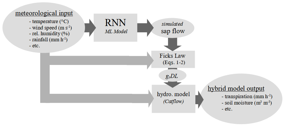
Figure 2Flow chart of the hybrid model that combines a recurrent neural network (RNN) and a process-based hydrological model to estimate transpiration.
2.2.5 CATFLOW parameterization
We use the well-tested, representative hillslope model from Loritz et al. (2017, 2021) to simulate the water balance of the Weierbach using CATFLOW. The representative hillslope model was set up based on field data for the bedrock topography, soil properties, and surface topography. The model was fine-tuned by exclusively adjusting the spatially explicit macropore network (approach described in detail in Wienhöfer and Zehe, 2014) with the goal of matching the seasonal water balance and the hydrograph of the parenting Colpach catchment during the hydrological year, October 2013 to October 2014. Loritz et al. (2017) showed that the representative hillslope model predicts the hydrograph of the Weierbach with a Nash–Sutcliff efficiency (NSE) of ≈0.7 and a Kling–Gupta efficiency (KGE) of ≈0.8 for the hydrological year 2012–2013 (test period) and the hydrological year 2013–2014 (training period) individually.
The simulation period in this study starts on 1 April 2014 and runs until 31 October 2016. This is preceded by a model spin-up starting in October 2013 with initial states of 70 % volumetric water content. We are using the exact same parameterization as explained in detail in our previous studies (Loritz et al., 2017, 2021) and do no recalibration of any model parameters besides changes described above to estimate the canopy conductance.
3.1 Sap flow model–data integration provides realistic canopy conductance and water balance estimates for a temperate beech forest
The daily averaged canopy conductance (m s−1) inferred from the sap flow measurements (gc sap) and those estimated by the a priori parameterized CATFLOW built-in stomatal conductance equation (gc Jarvis) correlate well (Spearman's rank correlation between gc Jarvis and gc sap is 0.85; the Pearson correlation is 0.75), although gcJarvis estimates are on average lower and show less temporal fluctuations than gc sap (Fig. 1a). The latter is underpinned by a low KGE coefficient (Gupta et al., 2009) of 0.15 and an RMSE of 0.01 m s−1. The gc sap estimates are within a reasonable range for beech-dominated temperate forests and comparable to literature values using a similar approach (inverse Penman–Monteith equation) based on six beech trees in the Czech Republic (Su et al., 2019). Differences between gc Jarvis and gc sap are also reflected, although weaker, in the monthly transpiration estimates (Fig. 1b). The CATFLOW model variant using gc sap (model–data integration) estimates about 130 mm more transpiration compared to the benchmark model variant using gc Jarvis for all 3 hydrological years, with the largest monthly difference of 21 mm per month in May 2015 (31 mm of total rainfall in May 2015).
Implementing gc sap instead of gc Jarvis in CATFLOW has only a weak effect on simulated runoff with a slight decline of the NSE from 0.75 to 0.7 over the 3-year period. This decrease in predictive performance likely occurs because the macropore network was tuned to optimize the streamflow of the Weierbach with gc Jarvis and not gc sap. This entails that a better performance could likely be achieved by tuning the macropore network once more with gc sap. However, we do not to perform further CATFLOW calibrations because our goal is to demonstrate the value of sap flow data in improving transpiration and soil moisture estimates and do not aim to obtain the highest performance in streamflow simulation (Appendix A2).
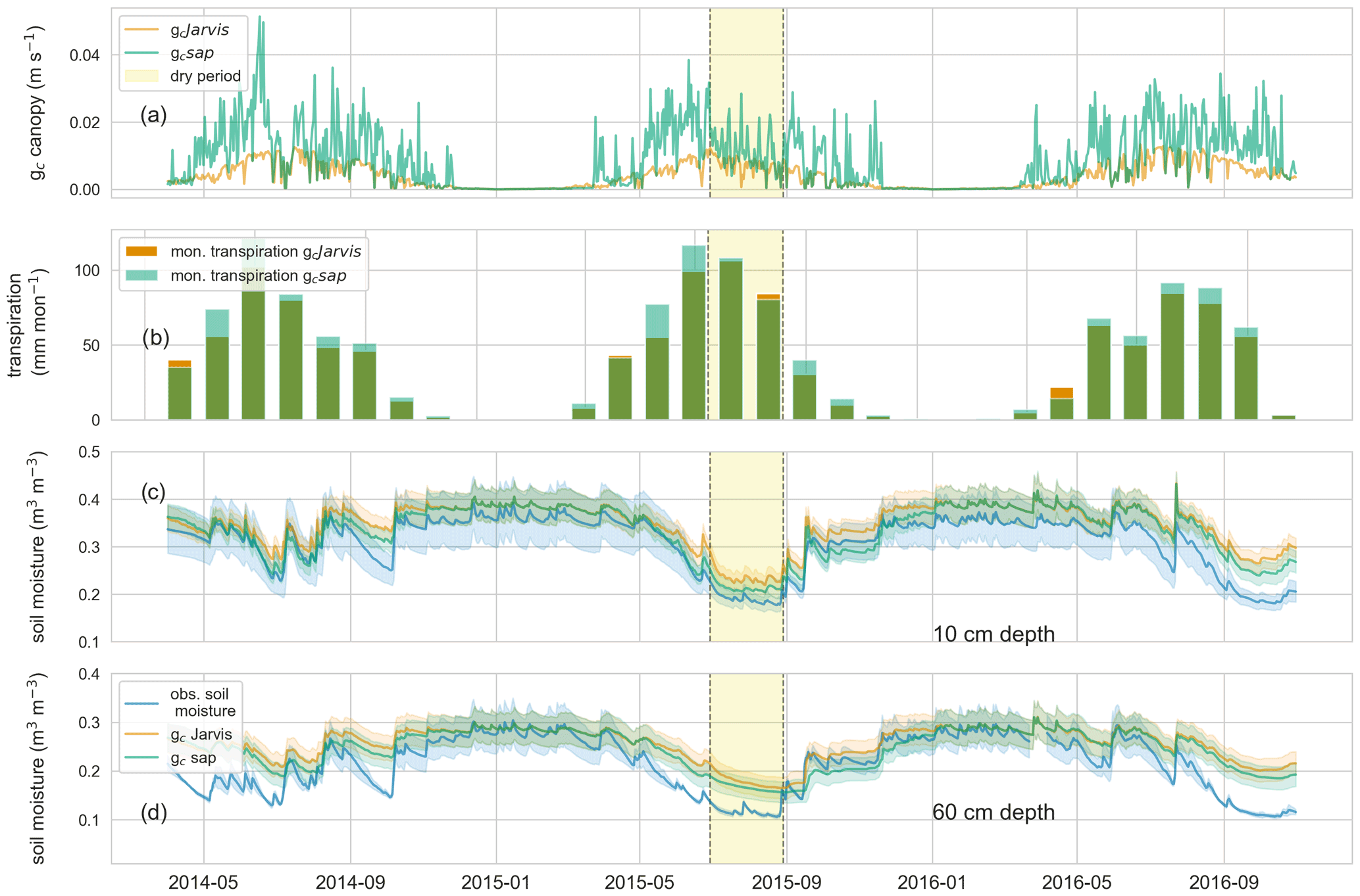
Figure 3(a) Daily averaged canopy conductance estimates for gc sap (green) and gc Jarvis (orange); (b) monthly transpiration sums estimated using gc sap (green) and gc Jarvis (orange); observed (blue) and simulated soil moisture ± standard deviation of the corresponding simulation and observations (gc sap: green; gc Jarvis: orange) at 10 (c) and 60 cm depth (d). Highlighted in yellow is a dry period from July to August 2015.
3.2 Ecohydrological simulations differ most during drought periods
Noticeable ecohydrological, relevant model improvements using gc sap occur during drought periods. For instance, 61 d of the 3-year record had close to no runoff (>0.001 mm h−1) observed in the Weierbach catchment. This period is only slightly overestimated by CATFLOW using gc sap (63 d), while it is substantially underestimated using the benchmark model with gc Jarvis (46 d). Both model variants (gc Jarvis and gc sap) correlate well with the observed soil moisture in 10 and 60 cm with Spearman's rank coefficients of around 0.9. However, simulations using gc sap result in overall lower soil moisture values with the largest difference in October 2015 (Fig. 1a and b). Using gc sap instead of gc Jarvis reduces the RMSE in the 2015 growing season from 0.033 to 0.01 (0.046 to 0.034) m3 m−3 at a 10 (and 60) cm depth. Furthermore, using gc sap instead of gc Jarvis leads to an average of about 2 mm less catchment storage after each of the three growing seasons. These storage differences are almost completely recharged during winter, typically until January, due to the wet autumns in the region. However, after the three growing seasons, the bedrock water storage (characterized by very low hydraulic conductivities and low porosities) is on average 2 % to 4 % lower when using gc sap compared to gc Jarvis after 3 years of simulations.
3.3 Recurrent neural networks (RNNs) accurately extrapolate sap flow data to different time periods and locations
Figure 3a displays hourly simulated sap flow (cm h−1) estimated by the deep-learning model against observed sap flow (cm h−1) at daytime (06:00 and 22:00 LT) of the growing season 2015 (test period). Simulated sap flow differs from observed sap flow by an RMSE of 0.8 cm h−1 during the training period (growing seasons 2014 and 2016) and 1.1 cm h−1 during the test period. If 2014 and 2015 are used as training period and 2016 as test period, the RMSE during the test period drops to 0.9 cm h−1, and if 2015 and 2016 are used as the training period and 2014 as the test period, the RMSE drops to 0.84 cm h−1. The Spearman's rank correlation between the observed and simulated sap flow in the test period is 0.91, indicating the ability of the deep-learning model to capture the general dynamics of sap flow using hourly meteorological data as predictors. Sap flow during the dry spell in July and August 2015 is on average overestimated by the deep-learning model. However, when adding 15 randomly picked continuous days of the dry period to the training sample (and removing those from the test sample), this bias and the RMSE are significantly reduced to 0.85 cm h−1. Furthermore, we also tested the ability of the deep-learning network to predict sap flow in a nearby catchment with a different geological and pedological setting but similar forest land cover. This first test suggests that the deep-learning network can predict sap flow in the test catchment, with lower errors than in the training catchment. This good out of sample performance points to the algorithm's ability to also extrapolate to higher unseen sap flows without further training (Appendix A1) while the test with the 15 randomly picked continuous days hints towards an inability of the ML approach to extrapolate to unseen dry conditions.
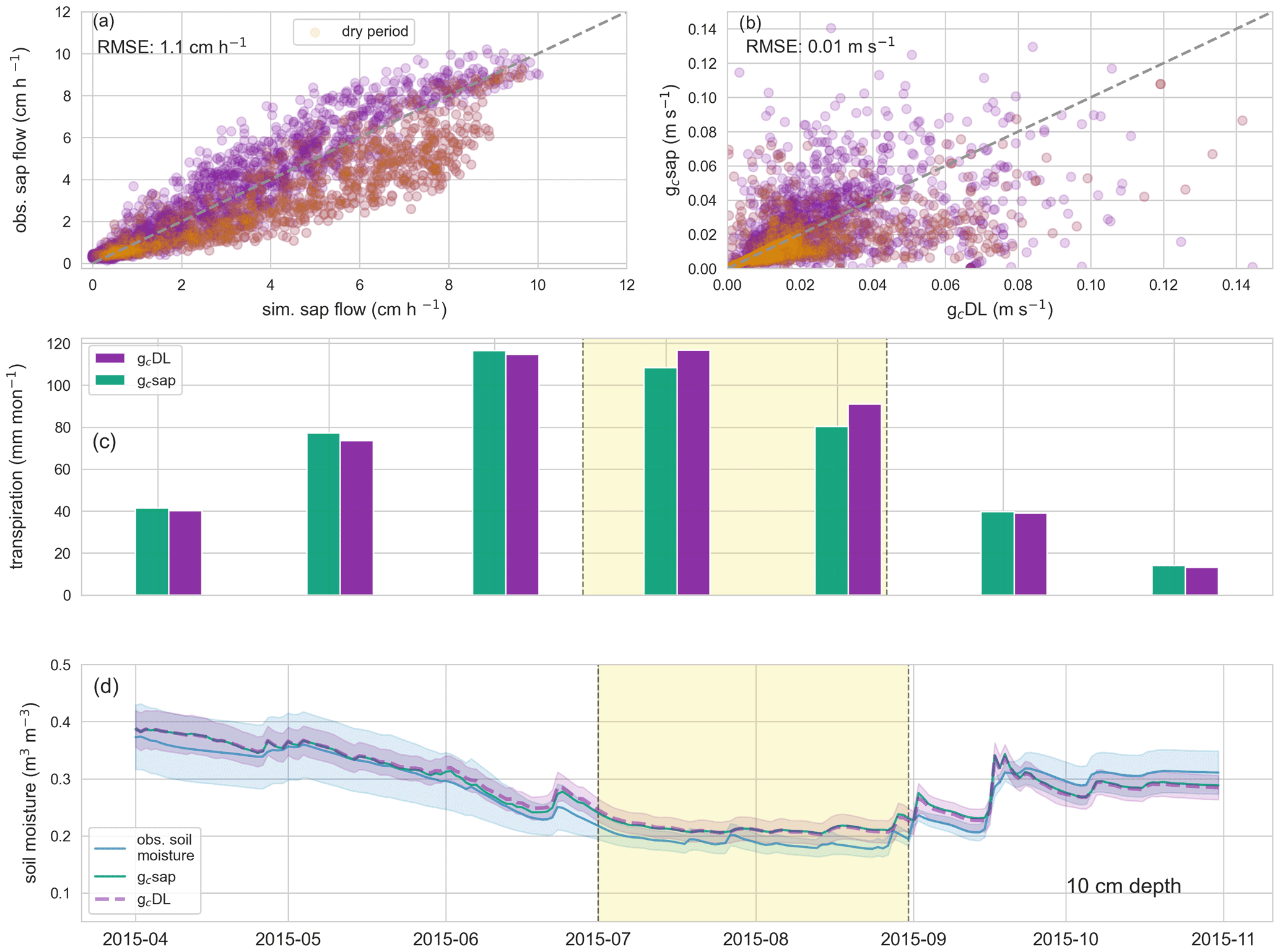
Figure 4(a) Hourly observed catchment-averaged sap flow and simulated sap flow in the growing season 2015; (b) hourly canopy conductances based on the hourly observed sap flow (gc sap) and simulated sap flow (gc DL); orange points in (a) and (b) are simulations or observations within the dry period of July and August 2015; (c) monthly transpiration sums estimated by gc sap (green) and gc DL (purple); (d) observed (blue) and simulated soil moisture (gc sap: green; gc DL: purple) in 20 cm. Highlighted in yellow is a dry period from July to August in the growing season 2015.
3.4 The hybrid model provides accurate canopy conductance and water balance estimates
The canopy conductance inferred from the observed sap flow (gc sap) and based on the simulated sap flow (gc DL) are compared in Fig. 4b. The two estimates differ by an RMSE of 0.01 m s−1 in the test period and have a Spearman's rank correlation of 0.9. The relation between the conductance estimates based on observed, (gc sap) and simulated (gc DL) sap flows is characterized by more and stronger outliers (residual larger than 0.025 m s−1, Fig. 4b). Note that more than 75 % of these outliers occur in the morning (06:00 to 10:00 LT) or evening time (16:00 to 22:00 LT). During these times, the Fick's law approximation is very sensitive to little changes in sap velocities, but transpiration is typically very low during these periods. This is further underpinned by the comparison of monthly transpiration sums displayed in Fig. 4c. The differences in using gc sap or gc DL are less than 3 mm per month during the majority of the growing season 2015 and increase to 7 and 9 mm per month in July and August only. During this period, sap flow, and to a smaller extent the corresponding gc values, are systematically overestimated by the RNN (Fig. 4a). As stated above, adding 15 dry days to the training data can reduce these biases and decrease the transpiration differences in July and August to below 4 mm per month. However, even without changing the training data of the RNN, the effect on simulated soil moisture dynamics is minor (Fig. 4d). This is because the model based on gc DL slightly underestimates transpiration in May and June, which is then compensated in July and August, and the simulated soil moisture from gc DL and gc sap differ only by an RMSE of 0.003 m3 m−3 in 20 cm and 0.002 m3 m−3 in 40 cm from 1 May to 31 October 2015.

Figure 5Hourly canopy conductances of gc sap (green), gc Jarvis (orange), and gc DL (purple) for 3 selected days in June, July, and August during the growing season 2015.
3.5 The hybrid model improves the diurnal cycle of canopy conductance compared to the benchmark model
Figure 5 shows three diurnal cycles of gc Jarvis, gc sap, and gc DL in June, July, and August. The gc sap is about twice as high in June compared to August and shows a stronger decline in conductance during midday in July and August. While such patterns are typical for humid forests under dry conditions (Su et al., 2019), they are not or only weakly captured by the Jarvis–Stewart model (gc Jarvis), which suggests a relatively constant conductance during daytime. As already indicated by the high correlation between gc DL and gc sap, the former also captures the dynamics of the diurnal cycles well. However, the gc DL model under- or overestimates several peaks, particularly during the morning and evening hours. This is in line with Fig. 4b and explains the larger spread of the gc estimates in contrast to sap flow predictions. The absolute cumulated difference of the transpiration estimates using either gc DL or gc sap in the chosen 3 d period is with 0.01, 0.014, and 0.07 mm d−1 low and highlights that errors in gc estimates in the morning and evening are less important for transpiration estimates.
4.1 Integrating sap flow data in a catchment-scale hydrological model
The comparison between both stomatal conductance models revealed that the a priori parameterized Jarvis–Stewart model (Jarvis, 1976; Stewart, 1988), in combination with the satellite-based VIIRS LAI values, clearly underestimated the canopy conductance, particularly during the spring and early summer. This bias could potentially be corrected by tuning the parameters of the Jarvis–Stewart equation. However, beyond revealing absolute errors in the seasonal cycle, the stomatal conductance model based on sap flow also demonstrates that the Jarvis–Stewart model is not able to reproduce diurnal hydraulic feedbacks along the soil–plant–atmosphere continuum reflected in the dips in canopy conductance during the midday water stress period. Mechanistic understanding of these stress responses in plant–water flow is still limited and representing them using existing ecophysiological models is challenging, especially beyond the individual tree (e.g., Grossiord et al., 2020; Kannenberg et al., 2022; Novick et al., 2019). On the other hand, these dynamics are embedded in the sap flow data and were adequately reproduced by the RNN for the purpose of hydrological modeling. The latter entails that the hybrid-model approach presented in this study may be more accessible to catchment hydrologist versus venturing too deep into the plant ecophysiological modeling with its promises and dangers. Therefore, learning this information from sap flow data with an RNN provides an avenue for catchment models to reproduce plant hydraulic behavior without explicitly parameterizing the soil–plant–atmosphere continuum at the catchment scale, which is complex and uncertain (Mencuccini et al., 2019).
Our results go beyond the established approach of estimating canopy conductance from sap flow data by directly integrating the data in a catchment-scale hydrological model and improving water balance simulations. Additionally, we can demonstrate the value of sap flow data in identifying suitable catchment-specific model parameterizations (Gupta et al., 1999) and show how the stomatal conductance model can be replaced by a model–data integration. Using the sap flow to calculate canopy conductance instead of transpiration has the advantage of omitting species-dependent errors in estimating the sap wood area and sap velocity distributions within the xylem. Faulty estimates of these parameters can lead to an overestimation of daily water use of up to 78 % for oak trees and −42 % in the case of oriental arborvitae trees as shown by Zhang et al. (2015). Nevertheless, the results of the RNN underpins the possibility to predict sap flow with an ML approach. This approach could then be extended to estimate transpiration based on catchment-averaged, species-dependent parameters, which could, for instance, be estimated by lidar measurements (Fassnacht et al., 2016).
4.2 Predicting canopy conductance using sap flow and an RNN
Recent studies have shown the large potential of decision tree-based ML algorithms for ecohydrological applications with a focus on predicting sap flow (Ellsäßer et al., 2020) or stomata conductances (Saunders et al., 2021) using meteorological data. In this study, we showed that RNNS are also suitable tools to predict sap flow by exclusively using meteorological variables as input. Only during the dry period in the growing season 2015, where the dormant trees most likely experienced water stress (Hoek van Dijke et al., 2019), the deep-learning network systematically overestimated sap flow. The latter was the reason to choose 2015 as test period and not 2016, which would have kept the chronological order and led to overall lower errors without bias. Initial tests reveal that adding 15 randomly picked continuous days during the drought period to the model training can reduce the residuals as well as the bias significantly, although soil moisture data were still not included as input. This indicates the potential of the RNN to mimic sap flow that is also under water stress and solely based on meteorological input. The latter entails that the information about the drought period is already within the meteorological input and different aggregations and combinations of the input variables, for instance, by estimating drought indices like the standardized precipitation index (SPI), could potentially further improve the prediction of sap flow under limited water availability. This study highlights the potential of the introduced deep-learning approach, but a more systematic investigation is required. Specifically, a next step could be to explore the potential of implementing the RNN such that the internal hydrological model states (especially soil water status) affect the sap flow predictions and the corresponding conductances. A similar hybrid-modeling approach has recently shown large potential to represent turbulent heat fluxes in hydrological models (Bennett and Nijssen, 2021).
4.3 Generalizing canopy conductance models based on sap flow data
This study is based on an unique data set with several sap flow sensors installed in different trees and locations as well as over several growing seasons (Hassler et al., 2018). Such data sets are labor-intensive and rare, although sap flow monitoring has become more common. While our proof of concept is limited to well-monitored experimental catchments, initial tests show that the RNN is capable of reproducing sap flow in a neighboring catchment, characterized by a similar forest structure but different hydropedological setting, even with lower residuals (Appendix A1). Approaches like transfer leaning, a concept to pretrain layers in a deep-learning network on a large data set and only fine tune a subset of these layers in the destination area, might be used to predict sap flow in a catchment with very little sap flow data available as well. Additionally, global and open data sets like SAPFLUXNET (Poyatos et al., 2016) in combination with catchment or forest properties offer opportunities to generalize our proposed approach. While ML predictions cannot directly advance understanding of the soil–plant–atmosphere continuum, we nevertheless show that they can be an improvement compared to reference empirical models that, if ill parameterized (Damour et al., 2010), are known to poorly capture non-linear responses of plant–water stress at the seasonal and diurnal time scales. Using ML sap flow predictions in combination with the inversed Fick's law offers the possibility to replace stomatal conductance models entirely in hydrological models.
The main findings from our study leveraging sap flow data and machine learning in a catchment-scale model are as follows:
-
Hourly, catchment-averaged sap flow can be used to estimate canopy conductance and inform a process-based hydrological catchment model to improve soil moisture and transpiration estimates.
-
Seasonal and diurnal model improvements were notable during drought periods when the reference empirical model underestimated plant–water stress and point to the valuable ecohydrological information encoded in sap flow data.
-
Recurrent neural networks are suitable tools to predict sap flow by exclusively using meteorological variables as input and offer promising avenues for developing generalized canopy conductance models for forward simulations beyond the monitoring time period and catchment location.
This study highlights the potential of sap flow data for improving hydrological simulations at the catchment scale by either constraining or informing hydrological models. We argue that sap flow sensors measure crucial information about one of the major fluxes of the hydrological cycle and should become the norm in experimental hydrology as soil moisture sensors, piezometers, or gauging stations are today already.
A1 Sap flow predictions in Huewelerbach
The Huewelerbach is a 2.7 km2 large headwater catchment located in Luxembourg within the experimental Attert basin (Pfister et al., 2002). The prevailing geology is sandstones above an impermeable layer of clay stones. It has a temperate semi-oceanic climate with a mean annual rainfall of 845 mm (Pfister et al., 2017) and mean monthly temperatures ranging between 0 ∘C in January and 17 ∘C in July. The catchment is entirely forested and dominated by deciduous beech trees. Meteorological data to run the recurrent neural network in this Appendix consisted of hourly global radiation (W m2), temperature (∘C), wind speed (m s−1), and relative humidity (%). Temperature and relative humidity are measured at a meteorological station located 3 km south of the catchment from a station operated by the “Administration des Services Techniques de l'Agriculture” (ASTA). Wind speed and global radiation are measured at a meteorological station in close proximity of the catchment that belonged to the CAOS project observation network.
We use sap flow velocities from one growing season (April–October 2015) measured within or in close proximity to the Huewelerbach catchment. Tree species consist of 27 beech trees (Fagus sylvatica), 7 oak trees (Quercus spec), and 2 hornbeams (Carpinus betulus) with individual tree diameter at breast height ranging from 22 to 91 cm (average 53 cm). Sap flow was measured and aggregated similarly as described in the method section.
Figure A1 shows the simulated and observed hourly sap flow in the Weierbach and Huewelerbach catchments for the growing season 2015. Sap flow was predicted using the same recurrent neural network trained exclusively in the Weierbach (growing season 2014 and 2016). There was no further change to that network. The recurrent neural network was capable of predicting sap flow in the Huewelerbach that was in better agreement with the observations than in the training catchment. One main reason for this performance increase is that, although they are in close proximity to the Weierbach, the dormant trees in the Huewelerbach did not experience water stress in 2015, most likely due to a large and accessible groundwater store (Hoek van Dijke et al., 2019). Other factors such as higher-quality meteorological data or (potential) sap flow data might also play a role but were not further investigated. Interestingly, the recurrent neural network is capable of simulating overall higher sap flow in the Huewelerbach, although such values have not been observed in the Weierbach. This supports the ability of the recurrent neural network to extrapolate in different sites.
A2 Comparison of the observed and simulated discharge
Figure A2 displays the observed discharge of the Weierbach catchment, the simulated discharge of the benchmark model (gc Jarvis), and the model–data integration that uses gc sap to estimate the transpiration. The performance of the model based on gc sap is reduced from an NSE of 0.75 to 0.7. The main difference between the two models are in the period after the growing season when the model that uses gc sap simulates too little discharge. Runoff generation in CATFLOW, particularly when the soil is dry, is significantly influenced by both the spatial explicit macropore network and the extent of the riparian zone. Hence, the decrease in predictive performance can likely be explained by the fact that the macropore network was tuned to optimize the streamflow of the Weierbach with gc Jarvis and not gc sap.

Figure A1(a) Hourly observed catchment-averaged sap flow and simulated sap flow in the growing season 2015 in the Weierbach catchment; (b) hourly observed catchment-averaged sap flow and simulated sap flow in the growing season 2015 in the Huewelerbach catchment; orange points in (a) and (b) are simulations or observations within the dry period of July and August 2015.
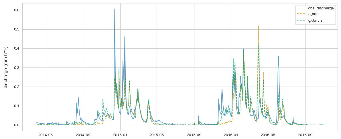
Figure A2Observed discharge of the Weierbach catchment, simulated discharge of the benchmark model (gc Jarvis), and simulated discharge of the model–data integration that uses gc sap to estimate transpiration.
Codes to estimate canopy conductance from sap flow and the RNN are publicly available at https://doi.org/10.5281/zenodo.6821189 (Loritz and Bassiouni, 2022). The meteorological data and the soil moisture data are also publicly available at https://doi.org/10.5281/zenodo.4537700 (Hissler et al., 2022). The sap flow data are available from Theresa Blume and Markus Weiler on request, however, a data publication is close to being finished. The link to the sap flow data publication will be added to https://doi.org/10.5281/zenodo.6821189 (Loritz and Bassiouni, 2022) in the near future.
RL and MB designed the study and wrote the paper. RL carried out all analysis and model simulations. SKH contributed expertise about sap flow measurements. AH and EZ contributed to interpreting results and editing the paper.
At least two of the (co-)authors are members of the editorial board of Hydrology and Earth System Sciences. The peer-review process was guided by an independent editor, and the authors also have no other competing interests to declare.
Publisher's note: Copernicus Publications remains neutral with regard to jurisdictional claims in published maps and institutional affiliations.
This research contributes to the Catchments As Organized Systems (CAOS) research group (FOR 1598), funded by the German Science Foundation (DFG ZE 533/11-1, ZE 533/12-1) in particular, sub-project G (Theresa Blume and Markus Weiler). Laurent Pfister and Jean-Francois Iffly from the Luxembourg Institute of Science and Technology (LIST) are acknowledged for organizing the permissions for the experiments and providing discharge data and the digital elevation model.
Maoya Bassiouni received funding from the European Commission and Swedish Research Council for Sustainable Development (FORMAS) (grant 2018-02787) in the frame of the international consortium iAqueduct, financed under the 2018 Joint call of the WaterWorks2017 ERA-NET Cofund. Ralf Loritz received funding by the Volkswagen Stiftung within the project “Invigorating Hydrological Science and Teaching: merging key Legacies with new Concepts and Paradigms (ViTamins)”.
The article processing charges for this open-access publication were covered by the Karlsruhe Institute of Technology (KIT).
This paper was edited by Markus Hrachowitz and reviewed by two anonymous referees.
Allen, R. G., Pereira, L. S., and Smith, M.: Crop evapotranspiration – Guidelines for computing crop water requirements, Rome, Italy, http://www.fao.org/3/X0490E/X0490E00.htm (last access: 27 September 2022), 1998.
Bennett, A. and Nijssen, B.: Deep Learned Process Parameterizations Provide Better Representations of Turbulent Heat Fluxes in Hydrologic Models, Water Resour. Res., 57, 1–14, https://doi.org/10.1029/2020WR029328, 2021.
Breuer, L., Eckhardt, K., and Frede, H.-G.: Plant parameter values for models in temperate climates, Ecol. Model., 169, 237–293, https://doi.org/10.1016/S0304-3800(03)00274-6, 2003.
Brown, A. E., Zhang, L., McMahon, T. A., Western, A. W., and Vertessy, R. A.: A review of paired catchment studies for determining changes in water yield resulting from alterations in vegetation, J. Hydrol., 310, 28–61, https://doi.org/10.1016/j.jhydrol.2004.12.010, 2005.
Burgess, S. S. O., Adams, M. A., Turner, N. C., Beverly, C. R., Ong, C. K., Khan, A. A. H., and Bleby, T. M.: An improved heat pulse method to measure low and reverse rates of sap flow in woody plants, Tree Physiol., 21, 589–598, https://doi.org/10.1093/treephys/21.9.589, 2001.
Campbell, G. S., Calissendorff, C., and Williams, J. H.: Probe for Measuring Soil Specific Heat Using A Heat-Pulse Method, Soil Sci. Soc. Am. J., 55, 291–293, https://doi.org/10.2136/sssaj1991.03615995005500010052x, 1991.
Damour, G., Simonneau, T., Cochard, H., and Urban, L.: An overview of models of stomatal conductance at the leaf level, Plant. Cell Environ., 33, 1419–1438, https://doi.org/10.1111/j.1365-3040.2010.02181.x, 2010.
Dingman, L. S.: Physical Hydrology, Waveland Press, Inc., ISBN 10: 1-4786-1118-9, ISBN 13: 978-1-4786-1118-9, 2015.
Duethmann, D., Blöschl, G., and Parajka, J.: Why does a conceptual hydrological model fail to correctly predict discharge changes in response to climate change?, Hydrol. Earth Syst. Sci., 24, 3493–3511, https://doi.org/10.5194/hess-24-3493-2020, 2020.
Dugas, W. A., Heuer, M. L., Hunsaker, D., Kimball, B. A., Lewin, K. F., Nagy, J., and Johnson, M.: Sap flow measurements of transpiration from cotton grown under ambient and enriched CO2 concentrations, Agr. Forest Meteorol., 70, 231–245, https://doi.org/10.1016/0168-1923(94)90060-4, 1994.
Ellsäßer, F., Röll, A., Ahongshangbam, J., Waite, P. A., Hendrayanto, Schuldt, B., and Hölscher, D.: Predicting tree sap flux and stomatal conductance from drone-recorded surface temperatures in a mixed agroforestry system-a machine learning approach, Remote Sens., 12, 1–20, https://doi.org/10.3390/rs12244070, 2020.
Ewers, B. E. and Oren, R.: Analyses of assumptions and errors in the calculation of stomatal conductance from sap flux measurements, Tree Physiol., 20, 579–589, https://doi.org/10.1093/treephys/20.9.579, 2000.
Fan, J., Zheng, J., Wu, L., and Zhang, F.: Estimation of daily maize transpiration using support vector machines, extreme gradient boosting, artificial and deep neural networks models, Agr. Water Manage., 245, 106547, https://doi.org/10.1016/j.agwat.2020.106547, 2021.
Fassnacht, F. E., Latifi, H., Stereńczak, K., Modzelewska, A., Lefsky, M., Waser, L. T., Straub, C., and Ghosh, A.: Review of studies on tree species classification from remotely sensed data, Remote Sens. Environ., 186, 64–87, https://doi.org/10.1016/j.rse.2016.08.013, 2016.
Gebauer, T., Horna, V., and Leuschner, C.: Variability in radial sap flux density patterns and sapwood area among seven co-occurring temperate broad-leaved tree species, Tree Physiol., 28, 1821–1830, https://doi.org/10.1093/treephys/28.12.1821, 2008.
Gharari, S., Gupta, H. V., Clark, M. P., Hrachowitz, M., Fenicia, F., Matgen, P., and Savenije, H. H. G.: Understanding the information content in the hierarchy of model development decisions: Learning from data, Water Resour. Res., 57, e2020WR027948, https://doi.org/10.1029/2020WR02794, 2021.
Granier, A. and Loustau, D.: Measuring and modelling the transpiration of a maritime pine canopy from sap-flow data, Agr. Forest Meteorol., 71, 61–81, https://doi.org/10.1016/0168-1923(94)90100-7, 1994.
Grossiord, C., Buckley, T. N., Cernusak, L. A., Novick, K. A., Poulter, B., Siegwolf, R. T. W., Sperry, J. S., and McDowell, N. G.: Plant responses to rising vapor pressure deficit, New Phytol., 226, 1550–1566, https://doi.org/10.1111/nph.16485, 2020.
Gupta, H. V., Bastidas, L. A., Sorooshian, S., Shuttleworth, W. J., and Yang, Z. L.: Parameter estimation of a land surface scheme using multicriteria methods, J. Geophys. Res.-Atmos., 104, 19491–19503, https://doi.org/10.1029/1999JD900154, 1999.
Gupta, H. V., Kling, H., Yilmaz, K. K., and Martinez, G. F.: Decomposition of the mean squared error and NSE performance criteria: Implications for improving hydrological modelling, J. Hydrol., 377, 80–91, https://doi.org/10.1016/j.jhydrol.2009.08.003, 2009.
Hassler, S. K., Weiler, M., and Blume, T.: Tree-, stand- and site-specific controls on landscape-scale patterns of transpiration, Hydrol. Earth Syst. Sci., 22, 13–30, https://doi.org/10.5194/hess-22-13-2018, 2018.
Hissler, C., Martínez-Carreras, N., Barnich, F., Gourdol, L., Iffly, J. F., Juilleret, J., Klaus, J., and Pfister, L.: The Weierbach experimental catchment in Luxembourg: A decade of critical zone monitoring in a temperate forest – from hydrological investigations to ecohydrological perspectives, Hydrol. Process., 35, 1–7, https://doi.org/10.1002/hyp.14140, 2021.
Hissler, C., Martínez-Carreras, N., Barnich, F., Gourdol, L., Iffly, J. F., Juilleret, J., Klaus, J., and Pfister, L.: The Weierbach Experimental Catchment (WEC) hydrological and isotopic database, Zenodo [data set], https://doi.org/10.5281/zenodo.4537700, 2022.
Hoek van Dijke, A. J., Mallick, K., Teuling, A. J., Schlerf, M., Machwitz, M., Hassler, S. K., Blume, T., and Herold, M.: Does the Normalized Difference Vegetation Index explain spatial and temporal variability in sap velocity in temperate forest ecosystems?, Hydrol. Earth Syst. Sci., 23, 2077–2091, https://doi.org/10.5194/hess-23-2077-2019, 2019.
Hrachowitz, M., Stockinger, M., Coenders-Gerrits, M., van der Ent, R., Bogena, H., Lücke, A., and Stumpp, C.: Reduction of vegetation-accessible water storage capacity after deforestation affects catchment travel time distributions and increases young water fractions in a headwater catchment, Hydrol. Earth Syst. Sci., 25, 4887–4915, https://doi.org/10.5194/hess-25-4887-2021, 2021.
Jackisch, C.: Linking structure and functioning of hydrological systems, KIT – Karlsruher Institut of Technology, https://doi.org/10.5445/IR/1000051494, 2015.
Jackisch, C., Knoblauch, S., Blume, T., Zehe, E., and Hassler, S. K.: Estimates of tree root water uptake from soil moisture profile dynamics, Biogeosciences, 17, 5787–5808, https://doi.org/10.5194/bg-17-5787-2020, 2020.
Jarvis, P. G.: The Interpretation of the Variations in Leaf Water Potential and Stomatal Conductance Found in Canopies in the Field, Philos. T. Roy. Soc. B, 273, 593–610, https://doi.org/10.1098/rstb.1976.0035, 1976.
Kannenberg, S. A., Guo, J. S., Novick, K. A., Anderegg, W. R. L., Feng, X., Kennedy, D., Konings, A. G., Martínez-Vilalta, J., and Matheny, A. M.: Opportunities, challenges and pitfalls in characterizing plant water-use strategies, Funct. Ecol., 36, 24–37, https://doi.org/10.1111/1365-2435.13945, 2022.
Köstner, B. M. M., Schulze, E. D., Kelliher, F. M., Hollinger, D. Y., Byers, J. N., Hunt, J. E., McSeveny, T. M., Meserth, R., and Weir, P. L.: Transpiration and canopy conductance in a pristine broad-leaved forest of Nothofagus: an analysis of xylem sap flow and eddy correlation measurements, Oecologia, 91, 350–359, https://doi.org/10.1007/BF00317623, 1992.
Loritz, R. and Bassiouni, M.: Leveraging sap flow data in a catchment-scale hybrid model to improve soil moisture and transpiration estimates, Zenodo [code], https://doi.org/10.5281/zenodo.6821189, 2020.
Loritz, R., Hassler, S. K., Jackisch, C., Allroggen, N., van Schaik, L., Wienhöfer, J., and Zehe, E.: Picturing and modeling catchments by representative hillslopes, Hydrol. Earth Syst. Sci., 21, 1225–1249, https://doi.org/10.5194/hess-21-1225-2017, 2017.
Loritz, R., Kleidon, A., Jackisch, C., Westhoff, M., Ehret, U., Gupta, H., and Zehe, E.: A topographic index explaining hydrological similarity by accounting for the joint controls of runoff formation, Hydrol. Earth Syst. Sci., 23, 3807–3821, https://doi.org/10.5194/hess-23-3807-2019, 2019.
Loritz, R., Hrachowitz, M., Neuper, M., and Zehe, E.: The role and value of distributed precipitation data in hydrological models, Hydrol. Earth Syst. Sci., 25, 147–167, https://doi.org/10.5194/hess-25-147-2021, 2021.
Maurer, T.: Physikalisch begründete zeitkontinuierliche Modellierung des Wassertransports in kleinen ländlichen Einzugsgebieten, Karlsruher Institut für Technologie, Karlsruhe, https://doi.org/10.5445/IR/65797, 1997.
Mencuccini, M., Manzoni, S., and Christoffersen, B.: Modelling water fluxes in plants: from tissues to biosphere, New Phytol., 222, 1207–1222, https://doi.org/10.1111/nph.15681, 2019.
Mendoza, P. A., Clark, M. P., Barlage, M., Rajagopalan, B., Samaniego, L., Abramowitz, G., and Gupta, H.: Are we unnecessarily constraining the agility of complex process-based models?, Water Resour. Res., 51, 716–728, https://doi.org/10.1002/2014WR015820, 2015.
Monteith, J. L. and Unsworth, M. H.: Principles of Environmental Physics, in: 4th Edn., Elsevier, ISBN 9780123869104, 2013.
Neill, A. J., Birkel, C., Maneta, M. P., Tetzlaff, D., and Soulsby, C.: Structural changes to forests during regeneration affect water flux partitioning, water ages and hydrological connectivity: Insights from tracer-aided ecohydrological modelling, Hydrol. Earth Syst. Sci., 25, 4861–4886, https://doi.org/10.5194/hess-25-4861-2021, 2021.
Novick, K. A., Konings, A. G., and Gentine, P.: Beyond soil water potential: An expanded view on isohydricity including land–atmosphere interactions and phenology, Plant Cell Environ., 42, 1802–1815, https://doi.org/10.1111/pce.13517, 2019.
Pfister, L., Iffly, J.-F., Hoffmann, L., and Humbert, J.: Use of regionalized stormflow coefficients with a view to hydroclimatological hazard mapping, Hydrolog. Sci. J., 47, 479–491, https://doi.org/10.1080/02626660209492948, 2002.
Pfister, L., Martínez-Carreras, N., Hissler, C., Klaus, J., Carrer, G. E., Stewart, M. K., and McDonnell, J. J.: Recent Trends in Rainfall-Runoff Characteristics in the Alzette River Basin, Luxembourg, Hydrol. Process., 31, 1828–1845, https://doi.org/10.1023/A:1005567808533, 2017.
Phillips, N. and Oren, R.: A comparison of daily representations of canopy conductance based on two conditional time-averaging methods and the dependence of daily conductance on environmental factors, Ann. Sci. Forest., 55, 217–235, https://doi.org/10.1051/forest:19980113, 1998.
Poyatos, R., Granda, V., Molowny-Horas, R., Mencuccini, M., Steppe, K., and Martínez-Vilalta, J.: SAPFLUXNET: Towards a global database of sap flow measurements, Tree Physiol., 36, 1449–1455, https://doi.org/10.1093/treephys/tpw110, 2016.
Reichstein, M., Camps-Valls, G., Stevens, B., Jung, M., Denzler, J., Carvalhais, N., and Prabhat: Deep learning and process understanding for data-driven Earth system science, Nature, 566, 195–204, https://doi.org/10.1038/s41586-019-0912-1, 2019.
Renner, M., Hassler, S. K., Blume, T., Weiler, M., Hildebrandt, A., Guderle, M., Schymanski, S. J., and Kleidon, A.: Dominant controls of transpiration along a hillslope transect inferred from ecohydrological measurements and thermodynamic limits, Hydrol. Earth Syst. Sci., 20, 2063–2083, https://doi.org/10.5194/hess-20-2063-2016, 2016.
Saunders, A., Drew, D. M., and Brink, W.: Machine learning models perform better than traditional empirical models for stomatal conductance when applied to multiple tree species across different forest biomes, Trees Forest. People, 6, 100139, https://doi.org/10.1016/j.tfp.2021.100139, 2021.
Seibert, S. P., Jackisch, C., Ehret, U., Pfister, L., and Zehe, E.: Unravelling abiotic and biotic controls on the seasonal water balance using data-driven dimensionless diagnostics, Hydrol. Earth Syst. Sci., 21, 2817–2841, https://doi.org/10.5194/hess-21-2817-2017, 2017.
Stewart, J.: Modelling surface conductance of pine forest, Agr. Forest. Meteorol., 43, 19–35, https://doi.org/10.1016/0168-1923(88)90003-2, 1988.
Stoy, P. C., El-Madany, T. S., Fisher, J. B., Gentine, P., Gerken, T., Good, S. P., Klosterhalfen, A., Liu, S., Miralles, D. G., Perez-Priego, O., Rigden, A. J., Skaggs, T. H., Wohlfahrt, G., Anderson, R. G., Coenders-Gerrits, A. M. J., Jung, M., Maes, W. H., Mammarella, I., Mauder, M., Migliavacca, M., Nelson, J. A., Poyatos, R., Reichstein, M., Scott, R. L., and Wolf, S.: Reviews and syntheses: Turning the challenges of partitioning ecosystem evaporation and transpiration into opportunities, Biogeosciences, 16, 3747–3775, https://doi.org/10.5194/bg-16-3747-2019, 2019.
Su, Y., Shao, W., Vlček, L., and Langhammer, J.: Ecohydrological behaviour of mountain beech forest: Quantification of stomatal conductance using sap flow measurements, Geosciences, 9, 243, https://doi.org/10.3390/geosciences9050243, 2019.
Tyree, M. T. and Ewers, F. W.: The hydraulic architecture of trees and other woody plants, New Phytol., 119, 345–360, https://doi.org/10.1111/j.1469-8137.1991.tb00035.x, 1991.
Wienhöfer, J. and Zehe, E.: Predicting subsurface stormflow response of a forested hillslope – the role of connected flow paths, Hydrol. Earth Syst. Sci., 18, 121–138, https://doi.org/10.5194/hess-18-121-2014, 2014.
Zehe, E., Maurer, T., Ihringer, J., and Plate, E.: Modeling water flow and mass transport in a loess catchment, Phys. Chem. Earth P. B, 26, 487–507, https://doi.org/10.1016/S1464-1909(01)00041-7, 2001.
Zehe, E., Ehret, U., Pfister, L., Blume, T., Schröder, B., Westhoff, M., Jackisch, C., Schymanski, S. J., Weiler, M., Schulz, K., Allroggen, N., Tronicke, J., van Schaik, L., Dietrich, P., Scherer, U., Eccard, J., Wulfmeyer, V., and Kleidon, A.: HESS Opinions: From response units to functional units: a thermodynamic reinterpretation of the HRU concept to link spatial organization and functioning of intermediate scale catchments, Hydrol. Earth Syst. Sci., 18, 4635–4655, https://doi.org/10.5194/hess-18-4635-2014, 2014.
Zhang, J.-G., He, Q.-Y., Shi, W.-Y., Otsuki, K., Yamanaka, N., and Du, S.: Radial variations in xylem sap flow and their effect on whole-tree water use estimates, Hydrol. Process., 29, 4993–5002, https://doi.org/10.1002/hyp.10465, 2015.
Zheng, J., Fan, J., Zhang, F., Wu, L., Zou, Y., and Zhuang, Q.: Estimation of rainfed maize transpiration under various mulching methods using modified Jarvis–Stewart model and hybrid support vector machine model with whale optimization algorithm, Agr. Water Manage., 249, 106799, https://doi.org/10.1016/j.agwat.2021.106799, 2021.