Present and future thermal regimes of intertidal groundwater springs in a threatened coastal ecosystem

In inland settings, groundwater discharge thermally modulates receiving surface water bodies and provides localized thermal refuges; however, the thermal influence of intertidal springs on coastal waters and their thermal sensitivity to climate change are not well studied. We addressed this knowledge gap with a field- and model-based study of a threatened coastal lagoon ecosystem in southeastern Canada. We paired analyses of drone-based thermal imagery with in situ thermal and hydrologic monitoring to estimate discharge to the lagoon from intertidal springs and groundwater-dominated streams in summer 2020. Results, which were generally supported by independent radon-based groundwater discharge estimates, revealed that combined summertime spring inflows (0.047 m³ s⁻¹) were comparable to combined stream inflows (0.050 m³ s⁻¹). Net advection values for the streams and springs were also comparable to each other but were 2 orders of magnitude less than the downwelling shortwave radiation across the lagoon. Although lagoon-scale thermal effects of groundwater inflows were small compared to atmospheric forcing, spring discharge dominated heat transfer at a local scale, creating pronounced cold-water plumes along the shoreline.

A numerical model was used to interpret measured groundwater temperature data and investigate seasonal and multi-decadal groundwater temperature patterns. Modelled seasonal temperatures were used to relate measured spring temperatures to their respective aquifer source depths, while multi-decadal simulations forced by historic and projected climate data were used to assess long-term groundwater warming. Based on the 2020–2100 climate scenarios (for which 5-year-averaged air temperature increased up to 4.32^∘), modelled 5-year-averaged subsurface temperatures increased 0.08–2.23^∘ in shallow groundwater (4.2 m depth) and 0.32–1.42^∘ in the deeper portion of the aquifer (13.9 m), indicating the depth dependency of warming. This study presents the first analysis of the thermal sensitivity of groundwater-dependent coastal ecosystems to climate change and indicates that coastal ecosystem management should consider potential impacts of groundwater warming.

1 Introduction

Global freshwater temperatures have been increasing in response to changes to climate and land cover (Desbruyères et al., 2017; IPCC, 2014; Isaak et al., 2017; Liu et al., 2020). Water temperature is a critical consideration in aquatic ecophysiology, as it influences the metabolic functions of all organisms (e.g., Morash et al., 2021) and the biogeochemistry of aquatic systems (Ouellet et al., 2020). Cold-water patches sourced by discrete groundwater inflows to streams form thermal refuges that enable heat-sensitive species to survive periods of elevated thermal stress (Kurylyk et al., 2015a; Sullivan et al., 2021; Torgersen et al., 2012; Wilbur et al., 2020). This cooling mechanism depends on the seasonal stability of groundwater temperature relative to surface water temperature due to the insulative effect of the ground overlying the source groundwater (Bonan, 2008). In addition to stable temperatures, focused groundwater discharge locations in surface water bodies are often characterized by distinct biogeochemical conditions preferred by certain aquatic species (Cantonati et al., 2020; Hayashi and Rosenberry, 2002). Although groundwater-dependent ecosystems may be more resilient to seasonal and short-term weather changes, they remain susceptible to multi-decadal warming signals that can penetrate deeper into the subsurface to affect groundwater temperatures (Bense and Kurylyk, 2017; Gunawardhana and Kazama, 2011; Menberg et al., 2014; Benz et al., 2022).

Surface water temperatures in inland lotic systems are influenced by latent, sensible, and radiative heat fluxes at the water surface, longitudinal heat flux along the channel due to advection and dispersion, and bed heat fluxes due to friction, conduction, and advection (Caissie, 2006; Dugdale et al., 2017), which in turn are controlled by landscape characteristics (O'Sullivan et al., 2019). The thermal regimes of many coastal aquatic systems are inherently more complex than freshwater systems as they are additionally influenced by exchanges with the ocean (e.g., Newton and Mudge, 2003). Furthermore, thermal stratification within coastal waters may arise due to salinity-induced density differences (e.g., Danielescu et al., 2009; Newton and Mudge, 2003; Nunes and Lennon, 1987). These complex thermal processes and patterns may contribute to the relative lack of study of coastal thermal regimes compared to inland lotic waters. However, a few studies have shown that net solar radiation, latent heat of evaporation, and sensible heat transfer to the atmosphere are typically the primary thermal drivers in shallow coastal waters (e.g., Ji, 2017; Rodríguez-Rodríguez and Moreno-Ostos, 2006).

Despite the large body of recent work and associated reviews characterizing river (Caissie, 2006; Dugdale et al., 2017; Ouellet et al., 2020), ocean (Abraham et al., 2013), and subsurface thermal regimes (Kurylyk et al., 2014a), relatively little work has focused on the influence of groundwater on the temperature of transitional coastal waters (e.g., Chikita et al., 2015; Rodríguez-Rodríguez and Moreno-Ostos, 2006). Groundwater may be delivered to the coast via direct (e.g., springs) and indirect (i.e., baseflow in streams or rivers) pathways and can influence coastal ecosystems (Luijendijk et al., 2020). As is the case for rivers, groundwater inputs to coastal environments may generate spatial thermal heterogeneity in the receiving water body (e.g., Danielescu et al., 2009; KarisAllen and Kurylyk, 2021), but the ability of these cold-water plumes to serve as thermal refuges is less explored. Further, although some riverine studies have considered the sensitivity of incoming groundwater to future climate change (e.g., Hannah and Garner, 2015; Kaandorp et al., 2019; Kurylyk et al., 2014b), to our knowledge no studies have investigated the thermal sensitivity of coastal groundwater discharge to climate change or the potential ecological consequences. Thermal sensitivity is broadly used in hydrology to refer to the change in water temperature due to atmospheric forcing (e.g., Kelleher et al., 2012). In the present context, thermal sensitivity refers to the change in groundwater temperature in response to climate change, which can be quantified as the ratio of the change in mean annual groundwater temperature to the change in mean annual air temperature (Kurylyk et al., 2015b).

Thermal imaging devices attached to aircraft have been used to aerially map thermal heterogeneity in coastal zones resulting from direct groundwater input (e.g., Coluccio et al., 2020; Danielescu et al., 2009; Lee et al., 2016a). Previous studies have utilized thermal infrared imagery to estimate local groundwater discharge via empirical relationships with thermal plume geometry (e.g., Bejannin et al., 2017; Danielescu et al., 2009; Kang et al., 2019; Kelly et al., 2019b; Lee et al., 2016a; Mundy et al., 2017; Tamborski et al., 2015). Small rotary-wing drones have the capacity to inexpensively collect thermal data with higher temporal and spatial resolution relative to conventional occupied aircraft (Dugdale et al., 2022; Lee et al., 2016b), although drone thermal data often involve additional challenges (e.g., thermal drift and limited spatial coverage; Dugdale et al., 2019; Kelly et al., 2019a). Despite these issues, this technology is suitable for determining relative temperature differences in individual images and thus can be used to locate focused groundwater inputs that generate anomalous water temperatures.

Knowledge gaps related to the hydrologic and thermal functioning of intertidal springs in coastal ecosystems and their thermal sensitivity to climate change provided the impetus for the present study. Our goals were to (1) quantify the discharge and present thermal influence of intertidal springs in a warm coastal lagoon ecosystem and (2) investigate how these springs will be thermally impacted by climate change using a numerical model informed by field data. Fieldwork and modelling work was conducted for a Marine Protected Area in eastern Canada with relatively high water temperatures (up to 33 ^∘C) and a thermally stressed ecosystem with an endemic strain of Irish moss. Drone thermal imaging was paired with in situ thermal and hydrologic monitoring to locate and further investigate spring and groundwater-dominated stream inputs to the lagoon. To interpret our measured spring temperatures and better understand how the aquifer and consequently the springs will respond to future warming, a numerical heat transfer model calibrated with groundwater data was applied to relate measured seasonal temperature signals at springs to their respective aquifer source depths and to simulate depth-dependent aquifer warming due to climate change. Field data and numerical modelling results were collectively used to assess our hypothesis that springs within this lagoon will be sourced from different depths and thus that some springs will manifest thermal impacts of climate change more quickly than others.

2 Site description

The study took place in the Basin Head lagoon on the eastern shore of Prince Edward Island (PEI) in Atlantic Canada (Fig. 1). The lagoon was established as a Marine Protected Area in 2005 under the Oceans Act to protect giant Irish moss, a unique morphotype of Irish moss (Chondrus crispus) endemic to the lagoon (DFO, 2009). The biomass of giant Irish moss within the lagoon declined by over 99 % from 1980 to 2008 (DFO, 2009), and thermal stress has been identified as one of the compounding stressors contributing to its decline (Joseph et al., 2021). Basin Head lagoon is approximately 0.6 km², with water depths that rarely exceed 2 m at high tide. The lagoon has a mixed semi-diurnal tide, with an average range of approximately 0.8 m, and is connected to the ocean by a narrow, artificial channel (Fig. 1b).

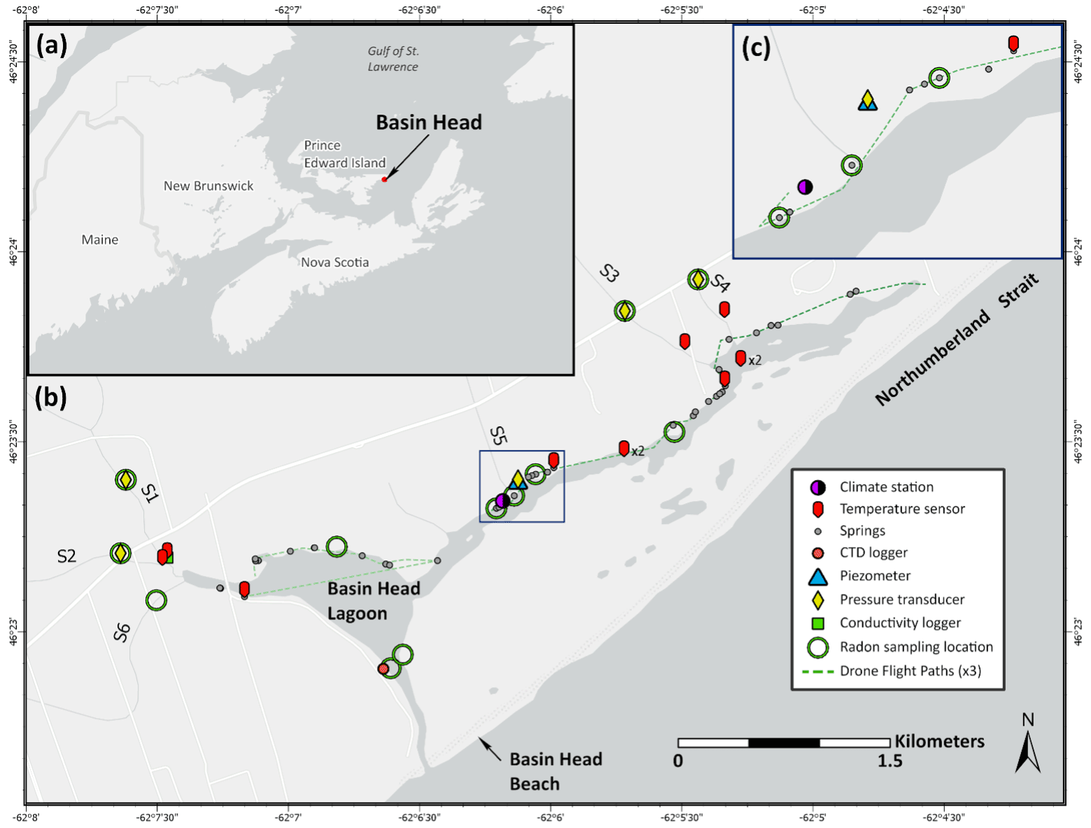
Figure 1 (a) Location of Basin Head lagoon within Atlantic Canada. (b) Instrument, radon sampling, and identified spring locations within Basin Head lagoon and watershed over the duration of the study. Temperature sensors installed in the northeast arm of the lagoon channel were in pairs (labelled as “×2”): one at the top (affixed to a buoy) and bottom (affixed to an anchor) of the water column. Drone surveying was performed in three flights (dashed green line) after scouting surveys identified spring locations. (c) Enlarged view of the densely instrumented area designated by the blue box in (b). CTD is conductivity, temperature, and depth. Basemap is attributed to Esri, HERE, Garmin, FAO, NOAA, USGS, © OpenStreetMap contributors 2000. Distributed under the Open Data Commons Open Database License (ODbL) v1.0.

PEI is characterized by mean annual precipitation ranging from 1046 to 1241 mm yr⁻¹ and mean monthly air temperatures from −7.9 to 18.6^∘ based on historical records of eight Environment and Climate Change Canada (ECCC) weather stations (Rivard et al., 2014). Precipitation is routed from the Basin Head watershed to the lagoon via groundwater-dominated streams (Fig. 1b) and direct groundwater discharge pathways. PEI bedrock aquifers are typically weakly consolidated, very fine to coarse, fractured sandstones with sparse occurrences of mudstone, conglomerate, and/or breccia (Brandon, 1966; Crowl, 1969a; van de Poll, 1989). Surficial tills within the study watershed are mainly clay–sand to sand-phase tills (Crowl, 1969b; Prest, 1973) and are estimated to be 5 m deep on average based on local core logs (Government of PEI, 2019).

3 Methods

Several methods were collectively used to test our primary hypothesis and undertake our objectives (Fig. 2). These are described in the following sections but are briefly summarized here to elucidate their interrelationships. Thermal-based drone mapping and analysis were used to identify spring locations and delineate the size of their thermal plumes (box 1; Fig. 2). Selected springs, streams, and a coastal piezometer (Fig. 1) were instrumented for in situ thermal and level monitoring (box 2). Thermal plume sizes (box 1) and flows (box 2) for selected springs underpinned an empirical relationship between plume area and spring discharge (box 3), which was applied to all springs to estimate total spring discharge to the lagoon (output 1). This total spring discharge was compared to total groundwater (springs plus non-point source diffusive flow) discharge estimates from a radon mass balance (box 4). The groundwater discharge estimates from thermal imagery were also used to estimate heat advection at the lagoon scale for the springs and streams (output 1) to assess their ecosystem impacts. Temperature data from a piezometer and well (box 2) were used in concert with climate data (box 5) to calibrate and drive a numerical model of groundwater temperature (box 6) for present and future climate conditions. Depth-dependent seasonal temperature signals in the calibrated model were compared to measured spring temperatures (box 2) to estimate the aquifer depths feeding those springs. Finally, simulated future groundwater temperatures (box 6) were used to provide insight into how springs sourced from different depths may warm in the future (output 2).

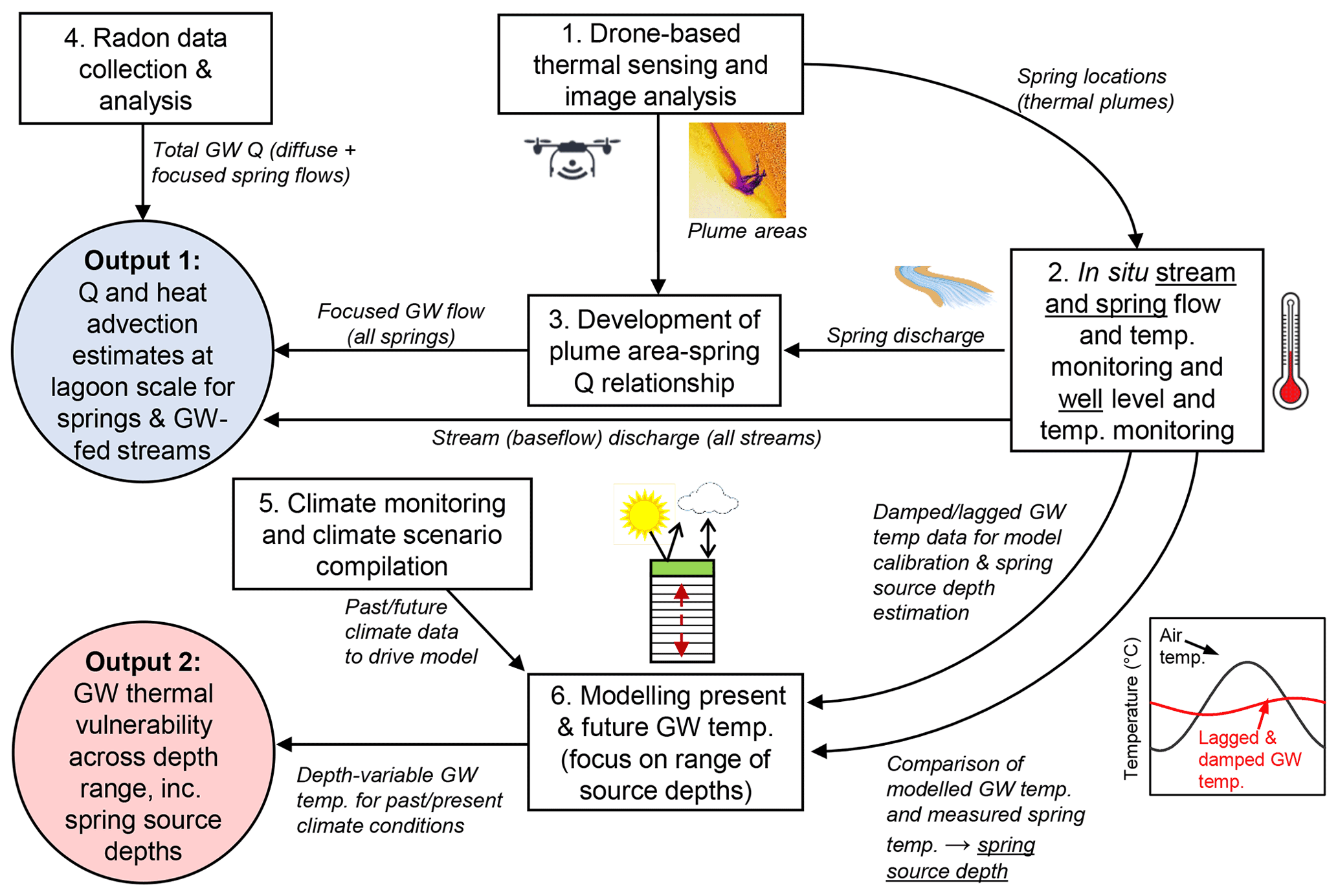
Figure 2 Diagram showing how the different aspects of this study are interrelated. Boxes indicate key study methods/elements, circles indicate key study outputs, and arrows and italicized text indicate outputs from one study element that become inputs for another. Q is discharge; GW is groundwater.

Fieldwork and data collection for this study occurred between June 2019 and November 2020. Lagoon water temperatures typically peak in July and August in the Basin Head lagoon, which reflects the period of greatest thermal stress for giant Irish moss. Contrast between groundwater and lagoon water temperatures is also greatest in July and August, which is favourable for the detection of springs via thermal infrared imaging. Accordingly, a dense network of sensors (Fig. 1) was temporarily installed between 23 July and 26 August 2020 (i.e., the 35 d “focused study period”), to provide a more detailed assessment of groundwater discharge during this critical period. Drone thermal images were captured in the summer of 2020, and radon sampling occurred during the summer and fall of 2020.

3.1 Remote thermal sensing and relationship to spring discharge

Stationary nadir thermal infrared images were taken (within 2 h of low tide, from an elevation of approximately 60 m a.s.l.) of the springs entering the lagoon throughout July and August 2020. This study used a Matrice 210 RTK v2 aerial drone, equipped with a 13 mm non-radiometric DJI ZENMUSE™ XT2 thermal infrared camera (DJI, 2018). Real-time kinetic processing was used for drone navigation (Kalacska et al., 2020). The exact temperatures of the thermal imagery were not deemed reliable due to internal drift of the sensor, lack of radiometric correction, and disagreement in thermal readings between frames. However, it was assumed that the relative temperature data in each frame were sufficiently precise for the consistent definition of thermal plume geometry, given the reproducible ability of the XT2 to identify surficial thermal anomalies confirmed with in situ temperature measurements. The image analysis process to identify thermal anomalies and delineate the associated cold-water plumes was based on previous work (e.g., Kelly et al., 2019; Roseen, 2002) and is described in the Supplement (Figs. S1 and S2).

Once the thermal plume areas were delineated, an empirical relationship was developed between discharge measurements for a subset of springs (Sect. 3.2) and their thermal plume areas (e.g., Danielescu et al., 2009). This plume area–spring discharge relationship was then applied to estimate the instantaneous discharge of all ungauged springs from their respective thermal plume areas captured by drone thermal imagery. Continuous spring discharge to the lagoon was estimated for the focused study period using a hydrologic proxy (e.g., Danielescu et al., 2009). Herein, the water levels in our near-shore piezometer (Fig. 1b and Sect. 3.2) were used as a proxy for the aquifer–lagoon hydraulic gradient and spring discharge (based on Darcy's law) via proportionality constants developed from the drone-based instantaneous discharge estimates (i.e., discharge was assumed to vary linearly with piezometer water table). Approximately 20 % of the lagoon's northwestern shoreline could not be surveyed with the drone based on proximity to the road or power lines (Fig. 1), but the presence of springs along this unsurveyed portion has been confirmed by distant thermal images and in situ measurements. Consequently, the total spring discharge to the lagoon was estimated by extrapolating the average spring discharge per shoreline length obtained from the surveyed segments (80 %) to the unsurveyed segment (20 %).

3.2 Hydroclimatic, thermal, and radon monitoring

The manufacturer, model, location, and monitoring durations for each logger are listed in Table S1, and locations are shown in Fig. 1. A climate station was installed at the study site to measure downwelling shortwave radiation, wind speed, rainfall, and air temperature. Subsurface modelling and hydraulic assessments were guided by in situ groundwater monitoring using a shallow groundwater piezometer (5 m a.s.l.; Fig. 1b) that fully penetrated the surficial soils to a depth of 4.5 m. This lowland well was instrumented with a pressure transducer to monitor well recovery during a slug test, as well as to provide a record of groundwater elevation, temperature, and electrical conductivity. Water stage was monitored at 15 min intervals in the four primary streams (S1 to S4; Fig. 1b) over the study period using pressure transducers corrected with air pressure data from the nearest ECCC climate stations (Station IDs 41903 and 7177; ECCC, 2021a, b). Stream discharges were measured using an acoustic Doppler velocimeter and were used to generate rating curves for local streams (average n= 6 and R²= 0.94). Other smaller streams (S5 and S6; Fig. 1b) were gauged intermittently, but their flow rates were < 1 % of the combined flow of streams S1 to S4 and are thus not considered hereafter. Considering the limited amount of precipitation (36 mm) over the 35 d focused study period (23 July to 26 August 2020), streamflows were assumed to be entirely baseflow. This simplification will be discussed later but is not anticipated to introduce significant error because PEI streams have frequently been documented to be 80 %–100 % baseflow during summer (Benson et al., 2007; Brandon, 1966).

A spring thermal plume area–discharge relationship (Sect. 3.1 and box 3; Fig. 2) in tidal zones is only valid for a point in time (i.e.., for a given tidal stage/current and atmospheric conditions) as the thermal and hydraulic mixing is highly sensitive to environmental conditions (KarisAllen and Kurylyk, 2021). Accordingly, we were only able to manually gauge three springs at approximately the same time as the lagoon-scale thermal mapping conducted on 22 July 2020. The environmental conditions were ideal for plume mapping and flow gauging on this date given the high (spring) tidal range that fully exposed the intertidal springs and the concurrent heat wave that maximized the thermal offset between the groundwater and lagoon. Volumetric flow measurements for these three springs (Figs. S3, S5) were conducted at low tide by constructing custom weirs surrounding their outlets. To remove any tide-circulated saltwater from our spring discharge estimates (LeRoux et al., 2021), the freshwater component discharging from the spring was isolated by estimating saltwater content via a simple two-component electrical conductivity mixing model. Importantly, while we only gauged three springs, the thermal plume areas for these springs span the range of all the mapped thermal plume areas but one. Thus, discharge rates for ungauged springs are generally interpolated rather than extrapolated from the plume area–discharge relationship.

Additional instruments were installed throughout the lagoon and watershed (Fig. 1) in tandem with stream monitoring work to investigate water quality and hydrologic and hydrodynamic processes. Temperature sensors were installed at multiple locations along the lagoon channel at the top (affixed to a buoy) and bottom (affixed to an anchor) of the water column, three springs outlets (i.e., Springs 2, 5, and 21; Figs. S3), and the four primary streams (Streams S1–S4) to characterize their thermal regimes. Spring temperature patterns (i.e., seasonal amplitudes) were compared to the results of the thermal numerical modelling (Sect. 3.3) to estimate the aquifer source depth for a given spring following the effective aquifer depth approach of Kurylyk et al. (2015b) and Briggs et al. (2018b). The paired spring flow and temperature data were used to quantify net (sensible) advective heat fluxes to the lagoon over the focused study period (Kurylyk et al., 2016):

$$\begin{array}{}\text{(1)}& J_{\mathrm{adv}}=C_{\mathrm{w}}{Q}_{\mathrm{input}}(T_{\mathrm{input}}-T_{\mathrm{lagoon}}),\end{array}$$

where J_adv is the net (sensible) advective energy flux (W), C_w is the volumetric heat capacity of water (J m⁻³ ${{}^{\circ }}^{-\mathrm{1}}$), Q_input is the input (direct rainfall, spring, or stream) water discharge (m³ s⁻¹), T is the water temperature (^∘), and T_input and T_lagoon are the water temperatures for the hydrologic input (rainfall, spring, or stream) and lagoon, respectively. Precipitation temperature was assumed to be the same as the average air temperature from the climate station over the short, focused study period. Advective heat fluxes for the springs and streams were considered to investigate the springs' thermal function at the scale of the lagoon. A complete lagoon energy balance cannot be completed due to a lack of complete surface energy flux data and data for the hydraulic and thermal exchange with the ocean. However, as a first-order estimate of the relative thermal effects of the freshwater inflows at the lagoon scale, the advective fluxes obtained via Eq. (1) were compared to the downwelling shortwave radiation (W m⁻²) measured at the study site climate station (Fig. 1) and multiplied across the lagoon surface area.

Conductivity–temperature–depth loggers were installed within the lagoon and in two intertidal springs (summer 2020 only). Discrete water temperature and electrical conductivity measurements of the lagoon, springs, streams, and piezometer were also taken during field investigations using handheld devices (Apera EC400S Portable Meter and a YSI ProDSS) to parameterize the two-component salinity mixing model used to correct the estimations of freshwater discharge from gauged springs.

Dissolved radon (²²²Rn; $t_{\mathrm{1}/\mathrm{2}}=$ 3.83 d) is naturally enriched in groundwater and is an inert noble gas, making it an effective tracer for groundwater discharge to coastal systems (Swarzenski, 2007). Four groundwater springs were sampled for ²²²Rn in August and November 2020 (Fig. 1b) coincident with continuous paired electrical conductivity, water depth, and temperature monitoring, as previously described. Glass bottles (250 mL) were submerged directly at the spring outlet and allowed to overflow, collecting bubble-free without headspace, and analyzed via RAD-H2O (Durridge Co.). Stream surface waters and shallow lagoon porewaters were additionally analyzed in November (Fig. 1b). Near the inlet of Basin Head lagoon, surface water was continuously drawn into a gas exchange chamber (RAD-AQUA), and ²²²Rn was monitored using a commercial radon-in-air monitor (RAD7, Durridge Co.) over 24 h in August (Fig. 1b, southernmost blue ring). Dissolved ²²²Rn activities were determined using the solubility constants from Schubert et al. (2012) for temperature and salinity and corrected for instrument response delay.

A mass balance model was developed for ²²²Rn (Burnett and Dulaiova, 2003; Rodellas et al., 2021; Sadat-Noori et al., 2015):

$$\begin{array}{}\text{(2)}& J_{\mathrm{mix}}+J_{\mathrm{decay}}+J_{\mathrm{atm}}=J_{\mathrm{spring}}+J_{\mathrm{stream}}+J_{\mathrm{diff}}+J_{\text{Ra-226}},\end{array}$$

where J represents the flux of ²²²Rn (Bq d⁻¹) for all known sources (baseflow-fed streams J_spring; molecular diffusion J_diff; ²²⁶Ra production J_Ra-226) and sinks (mixing J_mix; radioactive decay J_decay; atmospheric evasion J_atm) of ²²²Rn within the Basin Head lagoon. With the time-series monitoring station near the inlet of the lagoon, we assume that this point-in-space is representative of all ²²²Rn inputs and outputs through the tidal inlet, and thus any imbalance between known sources and sinks is attributed to unknown groundwater inputs (J_spring). This estimate provides a maximum range of groundwater inputs (Peterson et al., 2010) and includes both focused (springs) and diffuse groundwater discharge, in contrast with the thermal plume method (springs only).

3.3 Groundwater and thermal numerical modelling

Ground temperature modelling for present and future conditions was used to interpret field data and to project future groundwater warming (box 6; Fig. 2). A 1-D subsurface heat and water transport model was developed and manually calibrated to local groundwater temperature observations, with hydrologic parameterization informed by local data (e.g., weather data, piezometer slug test) and literature values, and calibrated using measured groundwater temperature data from the piezometer (Fig. 1) and an upland well (see Sect. 4.3.1). Downscaled future climate projections were then applied as upper-boundary conditions to drive simulations of plausible future subsurface temperatures, with the goal of assessing the potential sensitivity of springs to projected multidecadal warming trends (Fig. 3a). The conceptual complexity of the numerical model was limited both to facilitate model parameterization as well as interpretation; nevertheless, this approach preserved key heat transport processes. Multi-dimensional systems such as the fractured sandstone/mudstone aquifers feeding the intertidal springs in the Basin Head lagoon may be simplified into a one-dimensional system operating on the concept of an “effective aquifer depth”, which lumps together multi-dimensional processes and can be derived by relating the amplitude decay or phase shift of the seasonal groundwater temperature sinusoid relative to the air temperature signal (Kurylyk et al., 2015b). One-dimensional heat transfer modelling approaches have been used in previous studies considering groundwater thermal impacts on rivers (e.g., Briggs et al., 2018a, b) and in analytical solution studies of past or future groundwater warming (e.g., Gunawardhana et al., 2011; Irvine et al., 2017). The thermal regimes of shallow aquifers exhibit a depth-dependent response to seasonal surface temperature signals, and thus the measured seasonal amplitude of groundwater discharge temperature yields an approximate average groundwater depth (Kurylyk et al., 2015b) that can be used to estimate the thermal response of that spring to multi-decadal warming.

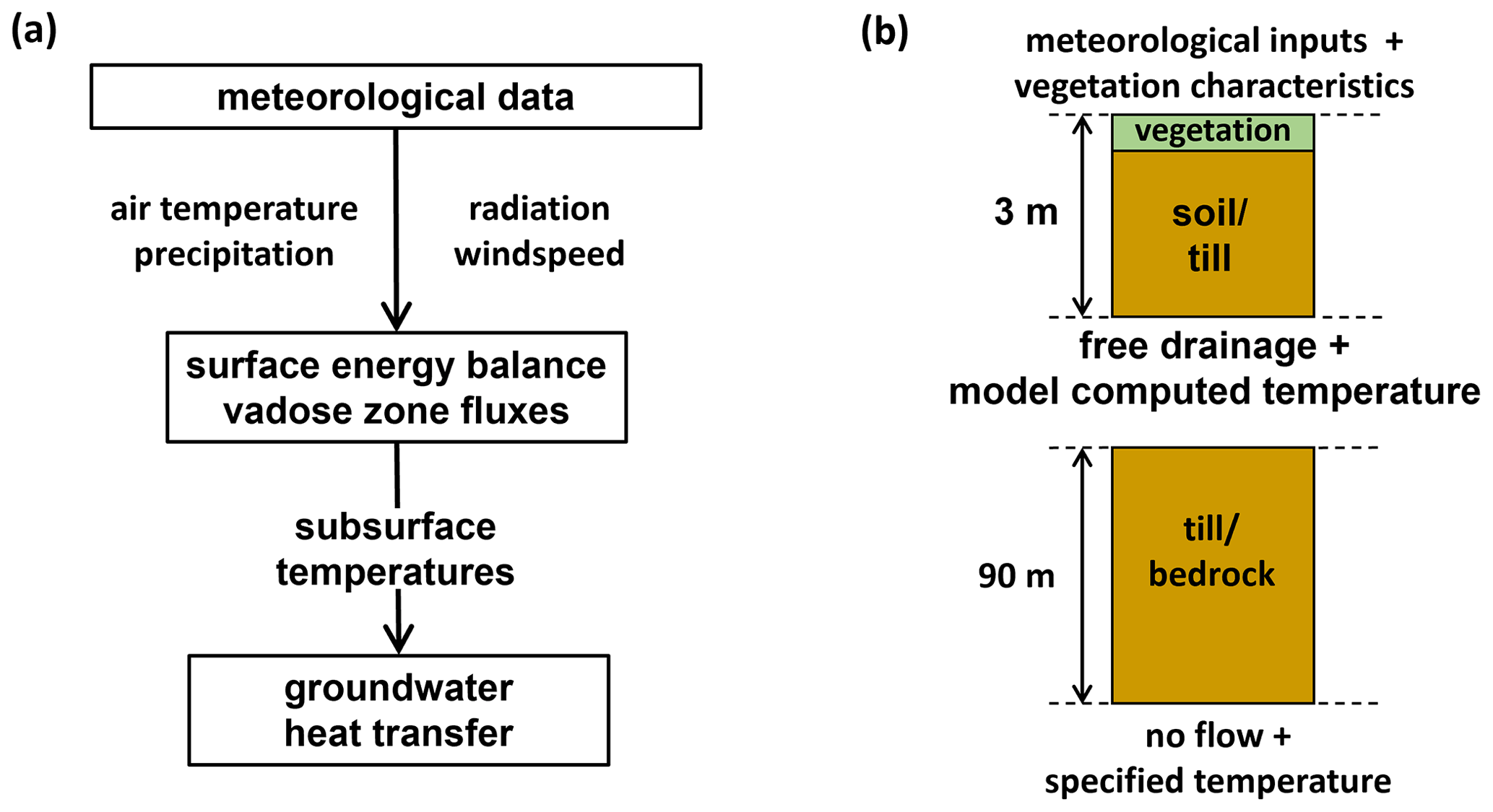
Figure 3 (a) Flowchart showing the conceptualization of the modelling approach used in this study and (b) conceptual diagram of SHAW model set-up and boundary conditions (not drawn to scale).

The selected model, Simultaneous Heat and Water model (SHAW; Flerchinger and Saxton, 1989), simulates transient vertical energy and water transport through a canopy, a snow layer, plant residue, and soil layers (Flerchinger, 2017). The robust physical basis and ability of SHAW to simulate the surface energy balance, snowpack, vegetation, and seasonally frozen soil processes (e.g., Mohammed et al., 2017) made it an appealing choice for this long-term thermal study, as these processes affect subsurface thermal trends at the latitude of the study site. A description of model processes and equations, as well as the boundary condition options, is detailed in Flerchinger (2017) and summarized here. The surface temperature (land, vegetation, or snow) is obtained by balancing the surface heat fluxes (net all-wave radiation, turbulent fluxes of sensible and latent heat, ground heat flux). Vertical heat transfer through the snowpack, vegetation, organic material, soil, and deeper subsurface layers is simulated with partial differential equations for energy transport. For the soil (ground) layers, the one-dimensional, transient conduction–advection equation in SHAW is

$$\begin{array}{}\text{(3)}& \begin{array}{rl}{C}_a{\displaystyle \frac{\partial T}{\partial t}}& -L_i{\mathit{\rho }}_{\mathrm{i}}{\displaystyle \frac{\partial {\mathit{\theta }}_i}{\partial t}}={\displaystyle \frac{\partial }{\partial z}}\left[{\mathit{\lambda }}_e{\displaystyle \frac{\partial T}{\partial z}}\right]-{\mathit{\rho }}_{\mathrm{w}}{c}_{\mathrm{w}}{\displaystyle \frac{\partial q_{\mathrm{w}}T}{\partial z}}\\ & -L_v\left({\displaystyle \frac{\partial q_{\mathrm{v}}}{\partial z}}+{\displaystyle \frac{\partial {\mathit{\rho }}_{\mathrm{v}}}{\partial t}}\right),\end{array}\end{array}$$

where C_a is the bulk volumetric heat capacity of the soil (J m^−3 ∘C⁻¹), T is soil temperature (^∘C), L_i is the latent heat of fusion (J kg⁻¹), ρ_i is the ice density (kg m⁻³), θ_i is the soil ice content (m³ m⁻³), λ_e is the bulk soil thermal conductivity (W m^−1 ∘C⁻¹), ρ_w is the water density (kg m⁻³), c_w is the water specific heat capacity (J kg^−1 ∘C⁻¹), L_v is the latent heat of vaporization (J kg⁻¹), q_w is the soil water flux (m s⁻¹), ρ_v is the vapour density in the soil (kg m⁻³), and q_v (kg m⁻² s⁻¹) is the soil vapour flux. Water balance and vertical fluxes are computed in a similar manner using a partial differential equation based on mass balance rather than energy balance (Flerchinger, 2017). SHAW has been successfully and widely applied in a range of environmental conditions to simulate subsurface temperatures.

Bulk thermal properties of the subsurface in SHAW are estimated based on the approach of DeVries (1963) using user-input soil compositions and model-computed water content; soil compositions were herein based on local soil surveys and historical studies of PEI soils (e.g., Crowl, 1969a). This study separated the model domain into an unsaturated upper region (0 to 3 m depth) that computed the upper-boundary condition and forcing to the lower, saturated region model (3 to 93 m depth; Fig. 3b). The bottom boundary position was selected (after various iterations) to ensure that the lower boundary did not influence the thermal sensitivity of the shallow groundwater temperatures, which were the focus of the present study. SHAW version 3.0.3 was used for the upper domain to calculate surface and vadose zone fluxes, whereas a modified version of SHAW 2.4 was used for the lower region to exclusively consider subsurface thermal transport below the water table without solving the surface energy balance (Mohammed et al., 2017).

Climate inputs required by SHAW to solve the surface energy balance for the upper region model include maximum and minimum daily air temperatures, dewpoint temperature, wind speed, total precipitation, and all-sky radiation. The time step, input data, and output of the simulations had a daily resolution as in other groundwater temperature studies using SHAW (e.g., Langford et al., 2020). Ground(water) temperatures in saturated conditions are relatively easy to simulate compared to soil moisture, which enables the coarser time step compared to models focusing on reproducing soil moisture variations. Based on the period of this study and the availability of historic data and climate projections, historical simulations were conducted over 37 years (1984–2020), and future simulations were run over 81 years (2020–2100). The minimum and maximum air temperatures, as well as total precipitation for the historical simulations, were sourced from the CNRM-CM5, RCP4.5 hindcast model (Voldoire et al., 2013), which more accurately reproduced historical conditions for PEI relative to other climate simulations (Warner, 2016). There is no direct long-term climate record for the study site (Basin Head), and, given our focus on multi-year averages in groundwater temperature, we are not concerned with high-frequency differences between hindcast data and actual environmental conditions. Thus, we used the hindcast data for our historical period (1984–2000). Data for the hindcast and projections were statistically downscaled to a ∼ 10 km grid size (ECCC et al., 2021c). Local dewpoint temperature, wind speed at 2 m above ground level, and all-sky solar radiation data were sourced from the NASA POWER reanalysis database (Sparks, 2018). As there were no readily accessible future projections for dewpoint temperature, wind speed, and all-sky solar radiation, these were estimated by repeating data from a portion of the historical period (i.e., 1985–2020; Sparks, 2018). The repetition of these data is not expected to produce significant errors given the relative hydraulic and thermal inertia of groundwater systems and because groundwater temperature changes are later interpreted herein using 5-year averages to smooth out any short-term effects. Future daily maximum air temperature, minimum air temperature, and total precipitation to drive future model projections were sourced from four climate simulations based on work by Warner (2016): (1) CNRM-CM5, RCP4.5; (2) CNRM-CM5, RCP8.5; (3) MRI-CGCM3, RCP4.5; and (4) MRI-CGCM3, RCP8.5 (ECCC et al., 2021c).

4 Results

4.1 Remote thermal sensing and spring discharge analysis

Based on cold-water plumes visible in the drone-based aerial thermal imagery (e.g., Fig. 4), 40 springs were located on the north and west shores of the lagoon (mapped in Fig. 1b and Figs. S2–S6 of the Supplement). Spring discharges were < 2 % saltwater, determined from electrical conductivity, so the resultant freshwater correction had a minimal effect on discharge estimates (Sect. 3.1, 3.2). The paired discharge values and thermal plume areas for the three gauged springs yielded a power function thermal plume area–discharge relationship for the lagoon at this point in time (R²= 0.99; Fig. 5d).

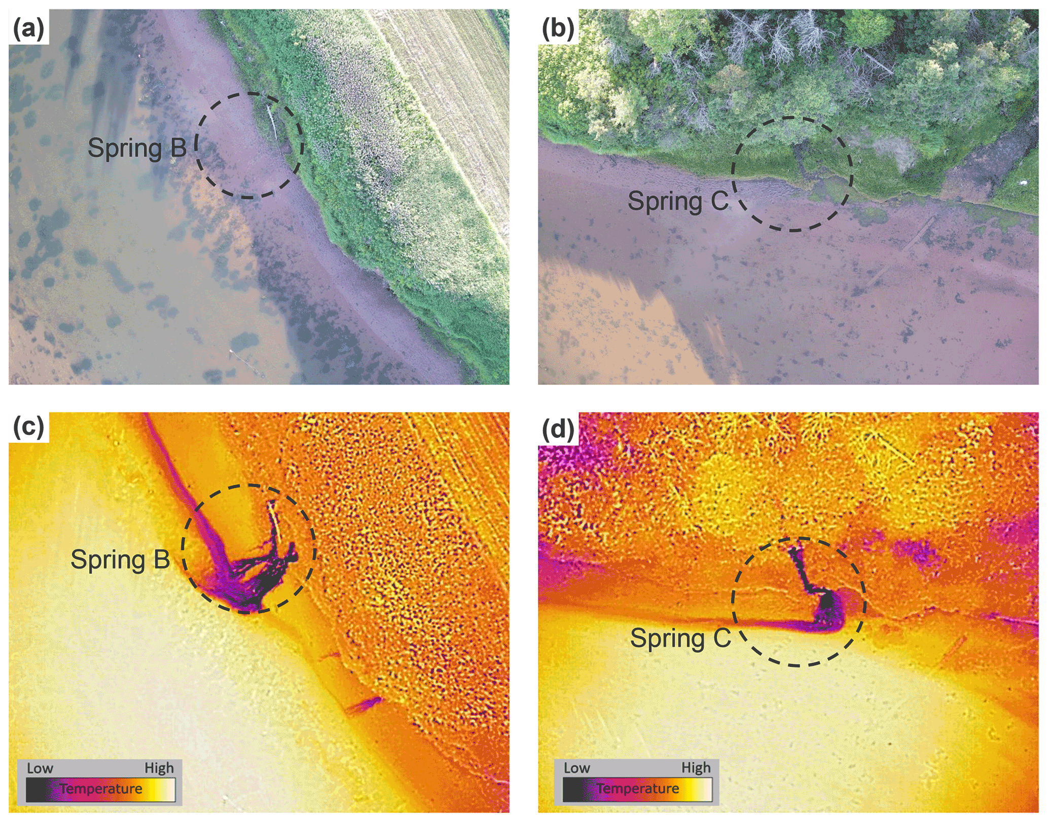
Figure 4 (a, b) Visual drone images of two of the springs that were manually gauged (Springs B and C; see Table S2). (c, d) Corresponding thermal images from the drone's thermal sensor. Scales are not equal among panels: there was a maximum thermal offset of 16 and 12^∘ between the spring water and receiving environment for (c) and (d), respectively. Pixel resolutions were 6.0 and 5.2 cm per pixel for panels (c) and (d), respectively.

Figure 5 Simplified workflow and results describing the area and discharge analyses of Spring 8 (included in Table S2 and Fig. S6) using the Basin Head plume size–spring discharge relationship. (a) Raw thermal image of Spring 8 cropped (rectangular) to the spring area (maximum offset of 14^∘ between the spring water and discharge environment; pixel resolution of 6 cm per pixel). (b) Thermal image converted to 8-bit grayscale and cropped (polygonal) to thermal groups of interest. (c) Graph of thermal image pixel data in terms of cumulative area and binned grayscale values. The graphical analysis method of Roseen (2002) guided by manual inspection of image pixel values was used to define the plume area (∼ 115 m²). (d) The plume size–spring discharge relationship from the three gauged springs of the lagoon is used to define spring instantaneous discharge based on plume area defined in (c). Panels (a), (b), (c), and (d) in this figure correspond with box numbers 1, 1b, 1c, and 3, respectively, for Fig. S1 in the Supplement.

The areas of only 34 springs were graphically assessed using low-tide thermal image pixel data (Table S2) because the remaining identified springs were either too small or inaccessible for close imaging via the drone. The workflow and results for the plume area associated with Spring 8 are shown as an illustrative example in Fig. 5. Instantaneous spring discharges for ungauged springs (Springs 1–31; Table S2) were computed as a function of plume area using the lagoon power function (Fig. 5d). The estimation of continuous spring discharge over the focused study period from the instantaneous spring discharges via the proxy data (i.e., piezometer water level, Sect. 3.2) yielded a total spring discharge volume estimate for this 35 d period of 113 000 m³ (0.037 m³ s⁻¹). Springs were found at a density of approximately six springs per kilometre along the surveyed section, which yielded approximately 580 m³ km⁻¹ d⁻¹ (0.0067 m³ s⁻¹ km⁻¹) for the discharge rate per shoreline length. Assuming a similar spring flow per length for the 20 % unsurveyed shoreline resulted in a cumulative 35 d total spring discharge of 142 000 m³ (0.047 m³ s⁻¹).

4.2 Hydroclimatic monitoring data and analyses

4.2.1 Stream discharge monitoring results

Stream monitoring data (Fig. S8) were analyzed to estimate the total indirect groundwater flow (baseflow) to the lagoon during the focused study period, which yielded the following inflow volumes (flows): S1 = 90 000 m³ (0.030 m³ s⁻¹), S2 = 22 000 (0.0073), S3 = 33 000 (0.011), and S4 = 7700 (0.0025). Based on the assumption that all streamflow is baseflow during the summer months as supported by the lack of flow “spikes” (Fig. S8) and typical summer conditions in PEI, streams contributed approximately 153 000 m³ (0.050 m³ s⁻¹) of indirect groundwater to the lagoon over the focused study period. This total streamflow is within 6 % of the total spring inflow estimated from the thermal analysis, suggesting the two hydrologic pathways for groundwater delivery (baseflow and spring discharge) are comparable at this site in the summer.

4.2.2 In situ temperature data

Water temperatures in the lagoon were relatively high during the focused study period (maximum 15 min temperature of 33 ^∘C), with mean daily water temperatures often greater than the mean daily air temperatures and occasionally exceeding 25 ^∘C in the northeast arm of the lagoon (Fig. 6). In contrast, the groundwater-dominated streams had mean daily water temperatures between 10 and 14 ^∘C during this period, and groundwater discharge temperatures remained between 7 and 10 ^∘C for all continuously monitored springs (Figs. 6, 7). Seasonal lagoon water temperatures peaked in late July to early August. Lagoon and stream temperatures exhibited at least limited diel variability (hourly data; Fig. S9), whereas none of the monitored springs displayed diel temperature fluctuations once tidal effects were removed. Over the focused period, the median 15 min water temperatures and interquartile ranges (IQRs) of Streams S1, S2, S3 and S4 were 8.7^∘ (IQR = 0.6^∘), 10.8^∘ (IQR = 1.2^∘), 10.5^∘ (IQR = 1.3^∘), and 10.4^∘ (IQR = 1.0^∘), respectively. Stream temperature measurements were taken near the stream mouths (above normal head of tide; Fig. 1) and represent the outcome of the cumulative upstream heat exchange, including the surface heat fluxes absorbed along the channel. This caused stream temperatures to exceed spring temperatures in the summer months (Figs. 6 and S9). Five temperature sensors distributed throughout the lagoon (Fig. 1b) over the focused period yielded a higher temperature median (∼22 ^∘C) and variability (IQR = 4^∘). Temperatures were typically greatest in the shallower, more poorly flushed upper reaches of the northeast arm of the lagoon and lowest in the deeper main basin (Figs. 1b, 6).

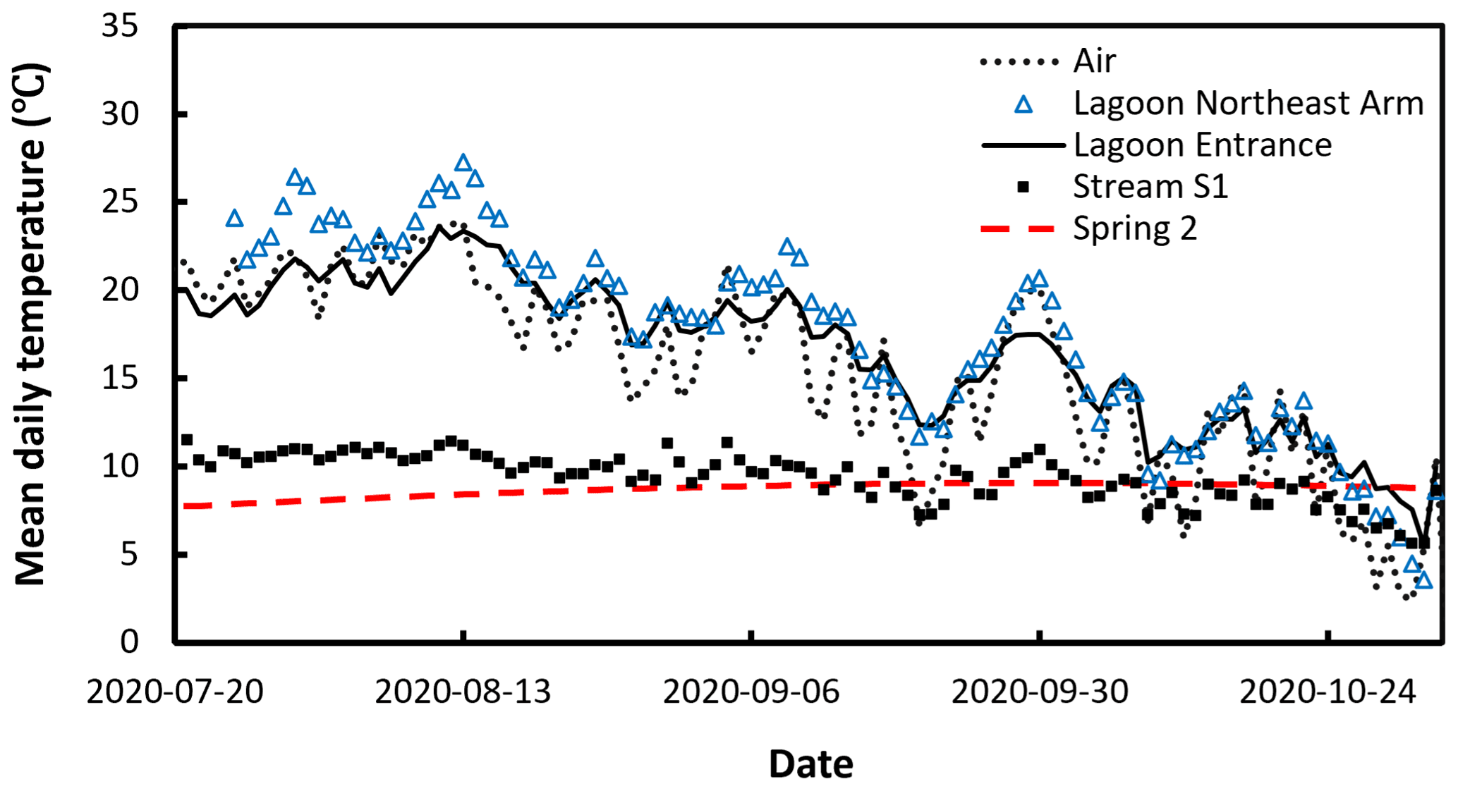
Figure 6 Illustrative examples (subset of monitored locations) of mean daily water temperatures vs. date (yyyy-mm-dd) for two locations in the Basin Head lagoon (i.e., entrance and northeast arm), Stream S1, and Spring 2 (with tidal effects corrected by considering the temperature only at low tide; see Fig. 7), as well as mean daily air temperature over the final 4 months of the study period. The lagoon northeast arm water temperature series was calculated from the average of two paired sensors (one at the lagoon water surface and the other at the channel bottom; see Fig. 1). The raw, uncorrected data and inferred annual groundwater temperature signal for Spring 2 are featured in Fig. 7c. Hourly data are in Fig. S9.

Summertime lagoon water temperatures over the study period were consistently lowered surrounding spring outlets; however, the extent of these thermal anomalies varied substantially with tidal stage and channel geometry (KarisAllen and Kurylyk, 2021). The difference between coincident spring and lagoon temperatures was up to 23^∘ (Fig. S9b). The thermal patterns of three springs (Fig. 7) were analyzed to estimate their seasonal signal properties (especially amplitude) and by extension their relative depth and vulnerability to climate warming by comparison to the modelled results. Temperatures at each of the spring outlets (Fig. 7) exhibited pronounced semi-diurnal oscillations (i.e., 12.42 h periods) due to the altered aquifer–lagoon hydraulic gradients and enhanced lagoon mixing at higher tide. To isolate the groundwater temperature from the time series at the spring outlets, the temperatures at low tide over several months of tidal cycles were fitted with an annual (period of 1 year) thermal sinusoid (dashed red lines; Fig. 7). The average temperature of Spring 5 was 7.65^∘ (Fig. 7a). The lack of thermal periodicity in this spring suggests that its source depth is below the extinction depth of annual air temperature patterns (normally 10–20 m in this region; e.g., Kurylyk et al., 2015b). In contrast, Spring 21 (Fig. 7b) displayed an annual signal with a mean of 7.75^∘ and an amplitude (half the range) of 1.6^∘. Spring 2 displayed a seasonal signal (Fig. 7c) with the lowest mean temperature (7.05^∘) and highest amplitude (2.0^∘). This amplitude suggests that Spring 2 has the lowest source depth and is the most vulnerable to multidecadal warming of the three springs investigated, as discussed later. The fitted spring temperature amplitudes were compared to depth-variable seasonal results from numerical modelling to infer approximate average depths of the groundwater delivered to the springs (Sect. 4.3.2).

Figure 7 Temperature data (black) from the mouths of (a) Spring 5, (b) Spring 21, and (c) Spring 2 (see Table S2 and Fig. S7 for locations) vs. date (yyyy-mm-dd) from Basin Head lagoon. The fitted annual temperature sine wave (GWT; in red) has a distinguishable amplitude in Springs 21 and 2 but not in Spring 5. GWT is the annual groundwater temperature waveform, and t is the time in days.

4.2.3 Lagoon heat fluxes

Selected advective components of the Basin Head lagoon heat budget associated with freshwater inflows were estimated for the 35 d focused study period (Table 1). Continuous spring discharge for the net advection calculation was estimated from the water table proxy approach (Sect. 3.2). The freshwater inflows from the precipitation, streams, and springs cooled the lagoon over the summer, as indicated by their negative net thermal advection values (Eq. 1) in Table 1. The estimated total net advective heat flows for the streams and springs were almost identical and over an order of magnitude higher than the advection from direct precipitation. Any unquantified diffuse groundwater input (upwelling to lagoon) would further increase the relative contribution of direct groundwater on the lagoon heat budget. As expected, heat flow from downwelling solar radiation was substantially higher than advective heat components to the lagoon (Table 1), suggesting that the springs and streams likely exert minor influence on the average water temperatures throughout the lagoon, despite their evident thermal impact at a localized scale along the shoreline (Figs. 4 and S8). A heat budget, including advective exchanges with the ocean and a complete surface energy balance, is required to gain a full understanding of the relative thermal effects of these freshwater inflows at the scale of the full lagoon, but data are not available for many heat flux components.

Table 1 Basin Head lagoon heat fluxes associated with three advective processes and downwelling shortwave radiation applied across the lagoon surface area. All heat budget components are over the 35 d focused study period. Positive values indicate an addition of sensible energy to the lagoon, while negative values indicate a cooling effect. Lagoon water temperature was approximated as its median value (22^∘) to calculate the advective terms (Eq. 1). n/a: not applicable.

4.2.4 Radon results

Near the lagoon inlet, surface water ²²²Rn activity varied from 10 to 97 Bq m⁻³, with maximum activities occurring near low tide when salinities were lowest and following classic hysteresis loops (Figs. 8a, b). The ²²²Rn activities of the fractured sandstone springs (10 400±3700 Bq m⁻³; n= 4) were an order of magnitude higher than for the shallow, brackish porewaters (630±250 Bq m⁻³; n= 4) and baseflow-fed streams (1100±1200 Bq m⁻³; n= 4), as shown in Fig. 8a and Table S3. Stream discharge during the surveyed period, 0.05 m³ s⁻¹, results in a stream-derived radon flux of (4.7±5.6) × 10⁶ Bq d⁻¹. This flux represents a theoretical maximum, as there will be appreciable ²²²Rn degassing and decay within the stream prior to entering the lagoon. Based on the minimum observed ²²²Rn concentration (Gilfedder et al., 2015), the diffusive flux of ²²²Rn may be approximated as 11±6 Bq m⁻² d⁻¹; or (6.4±3.2) × 10⁶ Bq d⁻¹, over the total lagoon area. Losses of ²²²Rn due to tidal mixing (Burnett and Dulaiova, 2003) and atmospheric evasion (MacIntyre et al., 1995) are taken as the mean (± standard deviation) losses estimated over the 24 h tidal cycle, upscaled to the lagoon surface area (Table S4). Similarly, radioactive decay is estimated considering the mean excess ²²²Rn inventory, for a net loss of (1.9±1.6) × 10⁶ Bq d⁻¹. Considering known sources and sinks, there is an excess of ²²²Rn ($\mathrm{8.0}\pm \mathrm{6.0}\times {\mathrm{10}}^{\mathrm{7}}$ Bq d⁻¹) attributable to groundwater. Using a ²²²Rn endmember from the fractured-sandstone springs (10 400±3700 Bq m⁻³), we estimate maximum groundwater inputs of 0.09±0.07 m³ s⁻¹. Given our uncertainties, the absolute value of this flux should be interpreted with caution, but it is useful for placing results from other methods into a broader context.

Figure 8 ²²²Rn variability versus salinity (a, b) and tidal water level (c), including hysteresis loops over two August 2020 tidal cycles; panel (b) depicts the lagoon data points outlined in (a) at a greater resolution. ²²²Rn values are listed in Table S3.

4.3 Groundwater and thermal numerical modelling results

4.3.1 Model calibration and sensitivity

Model elements (e.g., residue layer, organic content, water table depth, and snow/rain threshold) were manually calibrated within appropriate ranges to improve agreement of the historical simulation with the approximate calibration targets. The SHAW model was manually calibrated to the mean, amplitude, and lag of the seasonal groundwater temperature signal recorded in the transducer in the coastal piezometer (4.24 m below surface), and modelled and measured results were in agreement post calibration (Table S5). Furthermore, after accounting for the difference in water table depth, outputs from the calibrated model at 13.9 m depth were in agreement with temperature measurements at the same depth in a nearby upland provincial observation well (Souris Line Road observation well at 55 m a.s.l.; Government of PEI, 2021 and Table S1 footnote). Relative uncertainty results for the modelling are presented in Table S6.

4.3.2 Historic and future simulation results

The atmospheric forcing (Fig. 9a) and the SHAW-modelled subsurface temperature response (Fig. 9b) over the last 5 years (2016–2020) of the historical simulation are presented for different depths to illustrate the intra-annual variability of temperature and the attenuation and lagging of the surface temperature signal with depth. The modelled amplitudes of the annual temperature signals (Fig. 9) were compared to the measured spring outlet thermal patterns (red lines; Fig. 7) to estimate the springs' effective source depths. Based on their amplitudes, Springs 2 and 21 are likely predominantly sourced from effective depths between 3 and 7 m. Spring 5 is interpreted to be mostly fed from depths below 12 m, although we recognize that springs are sourced from the convolution of flows from different depths.

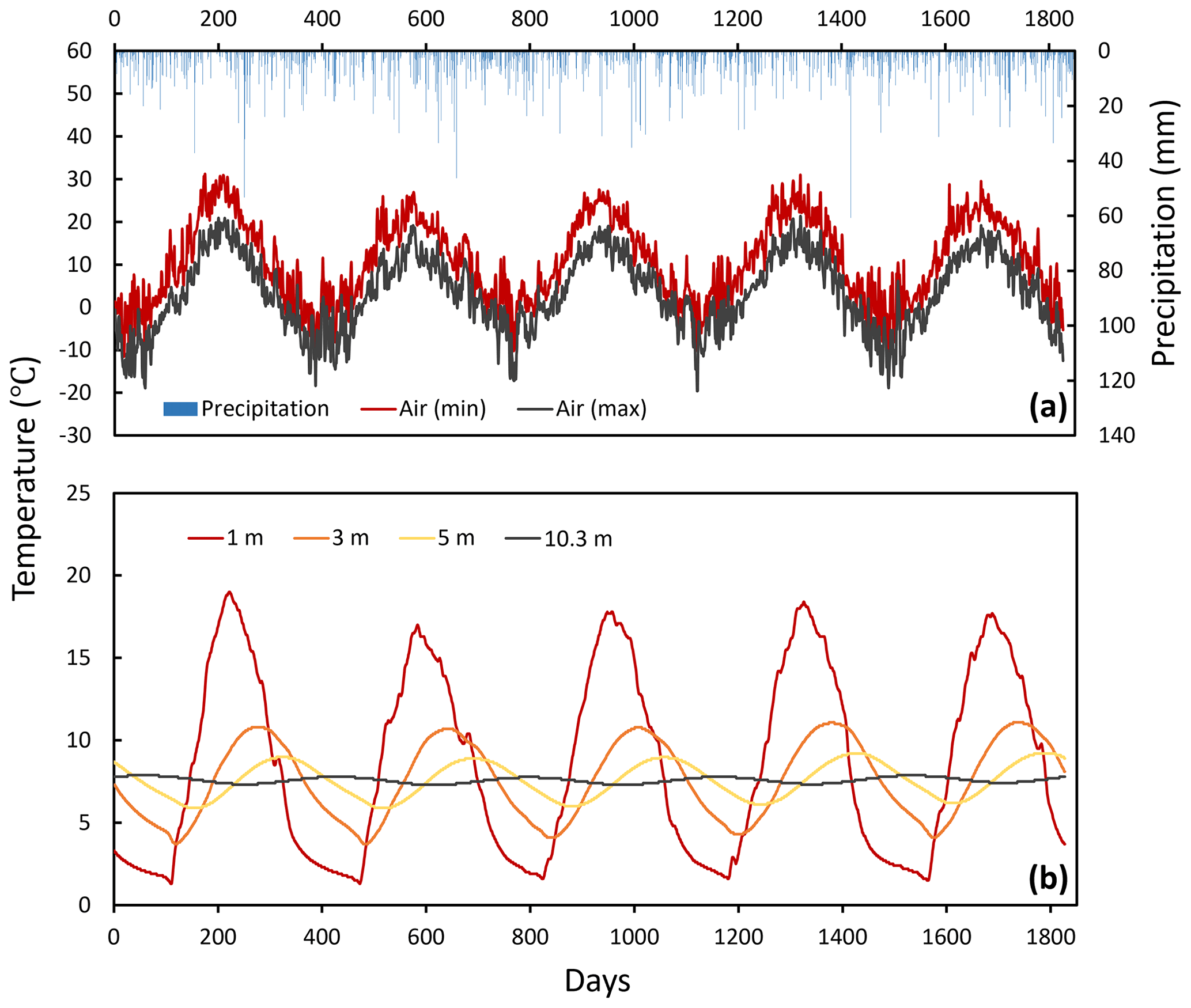
Figure 9 Historical simulation data for the years of 2016–2020 extracted from SHAW. (a) Maximum and minimum daily air temperature and total rainfall input to the model. (b) Subsurface temperatures at various depths in response to surface forcing. The temperature data at depths of 1 and 3 m were extracted from the surface domain, whereas the others are from the lower domain. Modelled amplitudes may be compared to measured spring signals to estimate their source depths.

The final 5 years of the future simulations (2096–2100) were compiled and compared to the final 5 years of the historical simulation (2016–2020, Table 2) to assess future groundwater warming. The subsurface temperatures at 4.2 and 13.9 m (sensor depths in piezometer and government well) increased with increasing atmospheric and surface temperatures in all simulations (Fig. 9). For example, focusing on the model calibration/assessment depths for the piezometer and monitoring well reveals that modelled groundwater temperature is projected to increase by 0.08 to 2.23^∘ at 4.2 m depth and by 0.45 to 1.62^∘ at 13.9 m (Table 2), indicating the depth dependency of warming for a given timeframe and the influence of a given climate scenario. The MRI-CGCM3, RCP8.5 simulation had the greatest temperature increase, whereas the MRI-CGCM3, RCP4.5 simulation had the lowest (Table 2).

Table 2 Simulated groundwater temperatures for the future SHAW simulations at the two studied depths (4.2 m is the piezometer sensor depth, while 13.9 m is the depth from provincial monitoring well sensor; see text). GCM is the global circulation model; RCP is the Representative Concentration Pathway. n/a: not applicable.

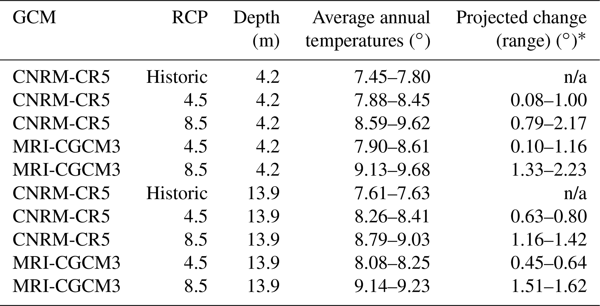
^* The projected temperature change was calculated by comparing the last 5 years of the future simulation to the last 5 years of the historic simulation.

The SHAW modelling indicates that the springs with more seasonally stable temperatures are sourced from greater depths (Fig. 9b) and will thus experience delayed warming due to climate change (e.g., Fig. 10a vs. b). For example, 5-year-averaged air temperature was simulated to increase by approximately 4.32^∘ over the course of the warmest future simulation (i.e., MRI-CGCM3, RCP8.5), which increased the 5-year-averaged groundwater temperature by approximately 1.78^∘ at 4.2 m depth and 1.57^∘ at 13.9 m depth. For comparison, this suggests a relative (to air) groundwater warming rate (or “thermal sensitivity”) of 0.41^∘ per degree of atmospheric warming at 4.2 m depth and 0.36^∘ per degree at 13.9 m depth by the year 2100, although the differences can be higher between these locations for a given year (see range in Table 2). The model results also illustrate that shallower aquifer zones are more vulnerable to short-term (seasonal and inter-annual) variations in temperature given how the seasonal amplitude and year-to-year variation are reduced with depth (Fig. 9b). Thus, short-term and long-term dynamics are more pronounced in shallower springs, causing them to reach higher peak temperatures in a given year.

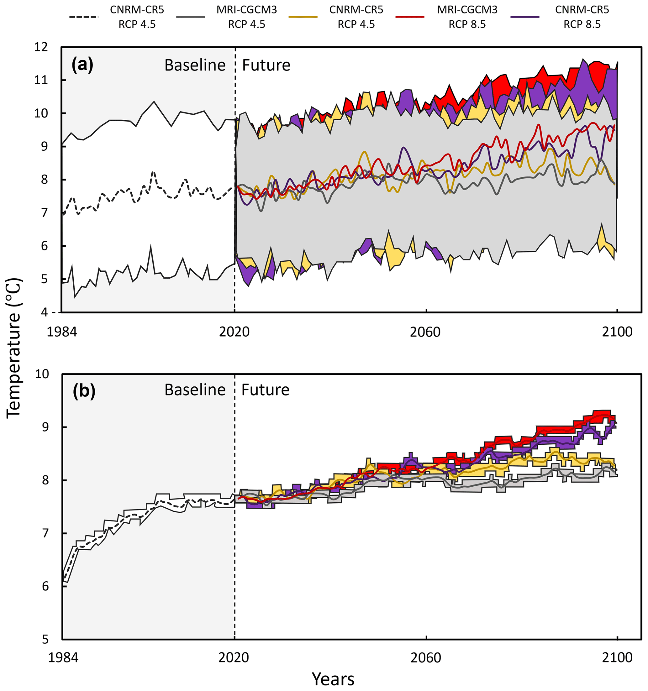
Figure 10 Modelled 365 d averaged subsurface temperatures (lines) and their associated intra-annual range (area) at two depths: (a) 4.2 m and (b) 13.9 m (representing the groundwater temperature sensor depths in our piezometer and the provincial monitoring well, respectively). The historical period (1984–2020) uses the CNRM-CR5 simulation data, and four future simulations were run for the period of 2020–2100. The beginning of the historical simulation involves a period of model domain stabilization.

5 Discussion

5.1 Thermal plume analysis and continuous discharge estimation

This study applied a power curve regression to the collected spring discharge and area data, which varies from previous studies that have applied linear (e.g., Bejannin et al., 2017; Lee et al., 2016b; Tamborski et al., 2015) or logarithmic relationships (Danielescu et al., 2009). Our high coefficient of determination (R²= 0.99; Fig. 5d) suggests a strong relationship between plume size and discharge, although we concede this is based on a limited number of points for reasons discussed. Previous studies have converted instantaneous discharge measurements based on thermal plume analysis to continuous discharge estimates using baseflow as a proxy for spring discharge (Bartlett, 2011; Danielescu et al., 2009). Rather than baseflow, we used groundwater levels measured in a piezometer close to the lagoon as this was thought to be a better proxy for the local hydraulic gradient (and thus spring flow) than baseflow, which integrates processes further up-catchment.

To overcome limitations with the limited number of points informing the thermal plume area–discharge relationship and the associated total spring discharge estimate of 0.047 m³ s⁻¹, we independently assessed total groundwater inputs using a ²²²Rn mass balance. Assuming that groundwater discharge to the lagoon accounted for the differences between known ²²²Rn sources and sinks, maximum input of groundwater was estimated as 0.09±0.07 m³ s⁻¹ (Table S4). Given the uncertainty of both approaches, these independent assessments are quite comparable. Also, the ²²²Rn approach may capture additional diffuse groundwater inflows not captured by the drone survey, and thus it is expected the discharge from the radon approach would be higher. For example, Danielescu et al. (2009) found that approximately 25 % of groundwater inflow to two PEI coastal systems was diffusive, and such inflows were not accounted for in the drone thermal imagery analysis in this study. The results reveal the value in using complementary but independent estimates of groundwater inflows from different types of tracers (heat and radon), particularly if both estimates are highly uncertain.

The comparison of estimated streams and spring flows from this study reveals that the magnitude of direct groundwater inputs to PEI coastal systems is likely significant relative to stream inputs in the summer. As in other studies (Danielescu et al., 2009), we assumed that intertidal spring discharge measurements taken at low tide were representative of the discharge over the tidal cycle. However, discharge would theoretically decrease at a higher stage due to the reduced aquifer–lagoon hydraulic gradient (Lee et al., 2016b; LeRoux et al., 2021), and spring-sourced thermal plumes at this site can be obscured at high tide (KarisAllen and Kurylyk, 2021). This is supported by time-series observations of ²²²Rn, where maximum activities are observed during ebb and low tides (Fig. 8c). However, relatively low electrical conductivity and temperature around certain springs during high tides suggests that at least some springs discharge continuously.

5.2 Water temperature and heat transfer

The thermal imagery and in situ temperature time series reveal the contrast between summer 2020 lagoon temperatures (mean $\sim \mathrm{22}{}^{\circ }$, maximum 33 ^∘C) and the stream (8–13 ^∘C) and spring temperatures (7–10^∘). The relative hydrologic and thermal stability of the streams attest to their groundwater dominance (Kelleher et al., 2012; Mayer, 2012; Johnson et al., 2020). The in situ data and thermal imagery also collectively illustrate that thermally stable groundwater inflows can reduce the temporal variability in surface water temperature (streams vs. lagoon temperatures; Fig. 6) and yet simultaneously enhance the spatial variability of temperature (lagoon cold-water patches). The influence of groundwater on the lagoon temperature relative to other thermal controls (e.g., tidal exchange and solar radiation) is dynamic in space and time. Groundwater inputs may be most significant as a thermal buffer throughout the hottest periods of the summer months when rainfall is scarce and lagoon temperatures and stream baseflow indices peak. A full lagoon energy budget (e.g., Rodríguez-Rodríguez and Moreno-Ostos, 2006) would improve our understanding of lagoon-scale thermal dynamics and thus the significance of groundwater and its sensitivity to climate warming. However, at a local scale, cold-water plumes created by intertidal springs can create distinct thermal zonation (e.g., Figs. 4, S8) that potentially provide thermal relief to aquatic organisms capable of behavioural thermoregulation or to static organisms collocated with the discharge point. While such groundwater-sourced, thermally habitable niches have received considerable attention in freshwater environments (e.g., Torgersen et al., 2012; Sullivan et al., 2021), they are less studied in transitional, coastal waters (Grzelak et al., 2018; Lecher and Mackey, 2018). The identified cold-water plumes are concentrated along the shoreline (Fig. 1), indicating that the nearshore zone and associated microecosystems may be more strongly influenced by focused groundwater inflows than the mid-lagoon waters.

5.3 Modelling implications

Intertidal springs in the lagoon are sourced from different effective depths in the groundwater system(s). Individual springs experience varied thermal forcing based on their associated soil layers, land use, land cover, and travel paths that dictate their thermal signature and sensitivity to surface temperatures. In this study, a one-dimensional subsurface model was used to demonstrate that springs within the lagoon are expected to warm in response to future atmospheric warming within decades. The reduced groundwater warming compared to atmospheric warming (Sect. 4.3.2 and Fig. 10) does not imply that aquifers ultimately attenuate multi-decadal surface warming signals but rather that there is a lag between a surface warming signal and its subsurface manifestation (Menberg et al., 2014; Bense and Kurylyk, 2017). For example, if the climate warmed to 2100 and then stabilized, the shallow aquifers over a range of depths would eventually be in equilibrium with the new thermal conditions, and the associated damping of groundwater warming relative to atmospheric warming would become progressively less apparent. It is also important to note that the lag in groundwater warming in response to climate change is not the same as the lag in response to seasonal forcing (Sect. 4.3.1) because the lag depends on the period of the forcing signal (e.g., Stallman, 1965). Modelling results suggest that the mean annual temperature of shallower groundwater supplying some springs may warm more than 2^∘ before the year 2100 (Table 2). The overall distribution of spring source depths would need to be further explored to assess how sensitive groundwater inputs to Basin Head lagoon may be at the lagoon scale, but these modelling results are valuable to understand the present/future system and to inform future research and management initiatives in this Marine Protected Area (Joseph et al., 2021).

Our modelling had several limitations. For example, we represented multi-dimensional processes in a one-dimensional system (Fig. 3) and did not have multi-depth groundwater data available at a single well for model assessment. Model uncertainty arose from uncertainty associated with the conceptual model, the thermal and hydraulic parameters, and the forcing data; however, ground temperature modelling is far more robust than soil moisture or groundwater hydraulics modelling because thermal signals are modulated with depth, and thermal properties are well constrained in comparison to hydraulic ones (Anderson, 2005). In general, considering the data availability and modelling objectives, the resulting calibration and model application were considered satisfactory for the investigations described above. However, future work could consider warming in a multi-dimensional aquifer system with responsive water table dynamics or more fully integrate the lagoon within the model domain in a coupled groundwater–surface water thermal modelling framework (e.g., Brookfield et al., 2009). Numerical groundwater models that account for secondary porosity could be used to consider heat transfer within the fracture network and the porous sandstone matrix (Graf and Therrien, 2007).

5.4 Ecological implications of spring warming

Springs are known to support critical groundwater-dependent ecosystems (Cantonati et al., 2020) due to the distinctive conditions (e.g., nutrient levels, dissolved oxygen, salinity, and temperature) at their outlets; this study focused on their thermal function. The significance of ambient or local lagoon temperature changes may be contextualized by species-specific temperature thresholds related to metabolic activity and survival. Optimal temperature for giant Irish moss is likely between 8 and 20^∘ (Bird et al., 1979; Mathieson and Burns, 1971; Tasende and Fraga, 1992), and temperatures above 30^∘ are highly detrimental (Kübler and Davison, 1993; Lüning et al., 1986). Furthermore, blue mussels (Mytilus edulis) provide essential anchorage to giant Irish moss (DFO, 2009; Joseph et al., 2021), and water temperatures above 25^∘ may encumber their growth and resilience to predation (Dowd and Somero, 2013). Increasing lagoon temperatures may also be anticipated to alter primary production and macroalgae bloom dynamics (Wells et al., 2020), as well as species distributions and interactions (Anderson, 2013). Consequently, warming of aquifers, and thus springs and groundwater-dependent streams, could negatively impact thermally vulnerable species, as mixing of groundwater into the lagoon results in lower summertime water temperatures at least locally and at low tide (Figs. 4 and S9). Also, fish have been observed aggregating in these cold-water plumes during warm days, perhaps suggesting that they are being used as refuges by thermally stressed aquatic species. Even with the groundwater warming presented in Table 2 and Fig. 10, discrete cold-water plumes will still be evident at the mouths of these springs in a warmer climate. However, in general, for a given spring and point in time, the plume volume under key temperature thresholds will be reduced by the multi-decadal warming in the aquifer and, presumably, the lagoon. In summary, because the drone imagery indicates that the thermal influence of certain springs and streams extends well beyond their outlets, groundwater warming and resultant plume warming could influence ecosystem complexity and dynamics within the broader lagoon in the coming decades.

6 Summary and conclusions

Groundwater-dependent coastal ecosystems are largely unexplored in the literature. This study used hydrologic and thermal monitoring, groundwater tracers (temperature and radon), and numerical modelling to explore groundwater discharge and its present and future roles in maintaining survivable temperatures for the threatened ecosystem in the Basin Head Marine Protected Area in southeastern Canada. The cold-water plume areas as revealed in drone-based thermal imagery were used to extrapolate the flow from three gauged springs to 31 ungauged springs. The cumulative spring inflow (0.047 m³ s⁻¹) estimated from this empirical approach was comparable to the total groundwater inflow (focused and diffuse, 0.09 m³ s⁻¹) yielded from a ²²²Rn mass balance. The results also revealed that the total spring flow was comparable to the total streamflow (0.050 m³ s⁻¹), suggesting that, at least at a local level, springs can provide an important pathway for delivering freshwater and energy to coastal zones. Based on a comparison to downwelling solar radiation, advection due to spring discharge exerted little influence on the lagoon-scale heat budget; however, thermal imagery indicates that the shoreline thermal regime is strongly influenced by groundwater discharge. The resultant thermal heterogeneity can provide thermal refuges to support a range of temperature tolerances in a complex ecosystem.

A subsurface heat transfer model parameterized and calibrated with field data was employed to investigate groundwater thermal sensitivity to seasonal cycles and multi-decadal climate change. The seasonal temperature amplitudes simulated at different depths for the historical period were compared to measured seasonal amplitudes from in situ spring monitoring, and this comparison indicated that the lagoon intertidal springs are sourced from a range of aquifer depths (from 4 m to more than 12 m). The response to seasonal forcing provided qualitative insight into how different springs within the same small lagoon may respond to multi-decadal forcing. Downscaled climate scenarios were used to drive future simulations to 2100, and the results revealed depth-dependent groundwater warming, with warming more pronounced at shallower depths (e.g., ≤ 2.23 ^∘C at 4.2 m) and less pronounced at greater depths (≤ 1.62 ^∘C warming at 13.9 m). The reduced warming with depth is a result of the depth-dependent lag between surface and groundwater warming signals. To our knowledge, no previous studies have investigated groundwater thermal sensitivity as a driver of future change in coastal lagoon ecosystems. Our results indicate that submarine or intertidal groundwater discharge sourced from shallow aquifers will likely experience non-negligible warming in this century and may strongly influence the shoreline ecosystem where springs are located. The interaction of spring discharge warming with lagoon changes due to sea-level rise and changing atmospheric forcing warrant further consideration and should be considered in future research using coupled thermal and hydrodynamic modelling. Future work could more fully integrate paired hydrologic and ecologic studies to better understand how resident species utilize spring-sourced thermal refuges.