the Creative Commons Attribution 4.0 License.
the Creative Commons Attribution 4.0 License.
 | 12 Aug 2022
Frozen soil hydrological modeling for a mountainous catchment northeast of the Qinghai–Tibet Plateau
Hongkai Gao
Chuntan Han
Rensheng Chen
Zijing Feng
Kang Wang
Fabrizio Fenicia
Hubert Savenije
Increased attention directed at frozen soil hydrology has been prompted by climate change. In spite of an increasing number of field measurements and modeling studies, the impact of frozen soil on hydrological processes at the catchment scale is still unclear. However, frozen soil hydrology models have mostly been developed based on a bottom-up approach, i.e., by aggregating prior knowledge at the pixel scale, which is an approach notoriously suffering from equifinality and data scarcity. Therefore, in this study, we explore the impact of frozen soil at the catchment scale, following a top-down approach, implying the following sequence: expert-driven data analysis → qualitative perceptual model → quantitative conceptual model → testing of model realism. The complex mountainous Hulu catchment, northeast of the Qinghai–Tibet Plateau (QTP), was selected as the study site. First, we diagnosed the impact of frozen soil on catchment hydrology, based on multi-source field observations, model discrepancy, and our expert knowledge. The following two new typical hydrograph properties were identified: the low runoff in the early thawing season (LRET) and the discontinuous baseflow recession (DBR). Second, we developed a perceptual frozen soil hydrological model to explain the LRET and DBR properties. Third, based on the perceptual model and a landscape-based modeling framework (FLEX-Topo), a semi-distributed conceptual frozen soil hydrological model (FLEX-Topo-FS) was developed. The results demonstrate that the FLEX-Topo-FS model can represent the effect of soil freeze–thaw processes on hydrologic connectivity and groundwater discharge and significantly improve hydrograph simulation, including the LRET and DBR events. Furthermore, its realism was confirmed by alternative multi-source and multi-scale observations, particularly the freezing and thawing front in the soil, the lower limit of permafrost, and the trends in groundwater level variation. To the best of our knowledge, this study is the first report of LRET and DBR processes in a mountainous frozen soil catchment. The FLEX-Topo-FS model is a novel conceptual frozen soil hydrological model which represents these complex processes and has the potential for wider use in the vast QTP and other cold mountainous regions.
- Article
(6783 KB) - Full-text XML
- BibTeX
- EndNote


1.1 Frozen soil hydrology: 1 of 23 unsolved problems
The Qinghai–Tibet Plateau (QTP) is largely covered by frozen soil and is characterized by a fragile cold and arid ecosystem (Immerzeel et al., 2010; Ding et al., 2020). As this region serves as the water tower for nearly 1.4 billion people, understanding the frozen soil hydrology is important for regional and downstream water resources management and ecosystem conservation. Frozen soil prevents vertical water flow, which often leads to saturated soil conditions in continuous permafrost, while confining subsurface flow through perennially unfrozen zones in discontinuous permafrost (Walvoord and Kurylyk, 2016). As an aquiclude layer, frozen soil substantially controls surface runoff and its hydraulic connection with groundwater. The freeze–thaw cycle in the active layer significantly impacts soil water movement direction, velocity, storage capacity, and hydraulic conductivity (Bui et al., 2020; Gao et al., 2021).
Frozen soil hydrology attracts increasing attention as the cold regions, e.g., QTP and the Arctic, are undergoing rapid changes (Song et al., 2020; Tananaev et al., 2020; Wang et al., 2017). Frozen soil thawing also poses great threats to the release of frozen carbon in both high-altitude and high-latitude regions, which is likely to create substantial impacts on the climate system (Wang et al., 2020). Attention to the impact of frozen soil hydrology on nutrient transport and organic matter and frozen soil–climate feedback is also growing (Tananaev et al., 2020). Hence, there are strong motivations to better understand frozen soil hydrological processes (Bring et al., 2016).
Frozen soil degradation and its impact on hydrology is one of the research frontiers for the hydrologic community (Blöschl et al., 2019; Zhao et al., 2020; Ding et al., 2020). The question of “How will cold region runoff and groundwater change in a warmer climate?” was identified by the International Association of Hydrological Sciences (IAHS) as being 1 of 23 major unsolved scientific problems (Blöschl et al., 2019) which requires stronger harmonization of community efforts.
1.2 The frontier of frozen soil hydrology
Knowledge on frozen soil hydrology was acquired through detailed investigations at isolated locations over various time spans by hydrologists and geocryologists (Woo, 2012; Gao et al., 2021). At the core scale, there are many measurements of soil profiles, including, but not limited to, soil temperature (Kurylyk et al., 2016; Han et al., 2018), soil moisture (Dobinski, 2011; Chang et al., 2015), groundwater fluctuation (Ma et al., 2017; Chiasson-Poirier et al., 2020), and active layer seasonal freeze–thaw processes (Wang et al., 2016; Farquharson et al., 2019). At the plot/hillslope scale, land surface energy and water fluxes are measured by eddy covariance, large aperture scintillometer (LAS), lysimeter, and multi-layers meteorological measurements. Geophysical detection technology allows us to measure various subsurface permafrost features (Wu et al., 2005). At the basin scale, except for traditional water level and runoff gauging, water sampling and the measurements of isotopes and chemistry components provide important complementary data to understand catchment-scale hydrological processes (Streletskiy et al., 2015; Ma et al., 2017; Yang et al., 2019). Remote sensing technology, including optical, near-infrared and thermal infrared, and passive and active microwave remote sensing, has been used to identify surface landscape features (e.g., vegetation and snow cover) and directly or indirectly retrieve subsurface variables (e.g., near-surface soil freeze–thaw and permafrost state) in frozen soil regions (Nitze et al., 2018; Jiang et al., 2020).
Besides measurement, modeling provides another indispensable dimension to understand frozen soil hydrology in an integrated way and make predictions of climate change. There has been a revival in the development of frozen soil hydrological models simulating coupled heat and water transfer. Such physically based models typically calculate seasonal freeze–thaw through solving heat transfer equations. Such equations are either solved analytically or numerically (Walvoord and Kurylyk, 2016). The Stefan equation is a typical example of the analytical approach, which calculates the depth from the ground surface to the thawing (freezing) horizon by the integral of ground surface temperature and soil features. The Stefan equation is widely used to estimate active layer thickness (Zhang et al., 2005; Xie and Gough, 2013) and is incorporated into some hydrological models (Wang et al., 2010; Fabre et al., 2017). The numerical solution schemes (e.g., finite difference, finite element, or finite volume) to model ground freezing and thawing is typically applied to one-dimensional infiltration into frozen soils and is included in models such as SHAW (Liu et al., 2013), CoupModel (Zhou et al., 2013), the distributed water–heat coupled (DWHC) model (Chen et al., 2018), the distributed ecohydrological model (GBEHM; Wang et al., 2018), and the three-dimensional SUTRA model (Evans et al., 2018). Andresen et al. (2020) compared eight permafrost models on soil moisture and hydrology projection across the major Arctic river basins and found that the projection varied strongly in magnitude and spatial pattern. Except for hydrological models, many land surface models explicitly consider the freeze–thaw process in order to improve land surface water and energy budget estimation and weather forecasting accuracy in frozen soil areas. Such models include VIC (Cuo et al., 2015), JULES (Chadburn et al., 2015), CLM (Niu and Yang, 2006; Oleson and Lawrence, 2013; Gao et al., 2019), CoLM (Xiao et al., 2013), Noah-MP (Li et al., 2020), and ORCHIDEE (Gouttevin et al., 2012). Comprehensive reviews on frozen soil hydrological models can be found in Walwoord and Kurylyk (2016), Jiang et al. (2020), and Gao et al. (2021).
1.3 The challenge of frozen soil hydrological modeling
Although numerous frozen soil hydrological models were developed, most models have strong prior assumptions on the impacts of frozen soil on hydrological behavior (Walvoord and Kurylyk, 2016; Gao et al., 2021). Such models follow a bottom-up modeling approach, which presents an upward or reductionist philosophy, based on the aggregation of small-scale processes and a priori perceptions (Jarvis, 1993; Sivapalan et al., 2003). However, most of the upward process understanding has been obtained from in situ observation and in situ modeling, which have limited spatial coverage and invariably limited temporal coverage (Brutsaert and Hiyama, 2012). It is worthwhile to note that frozen soil has tremendous spatiotemporal heterogeneities, which are strongly influenced by many intertwined factors, including, but not limited to, climate, topography, geology, soil texture, snow cover, and vegetation. Upscaling could average out some variables and turn other variables visible and even become dominant processes (Fenicia and McDonnell, 2022). Unfortunately, translating the spot-/hillslope-scale frozen soil process to its influence on catchment-scale hydrology, guided by carefully expert analysis and constrained by multi-source measurements, is still largely unexplored.
The effects of the soil freeze–thaw process on hydrology at the catchment scale is still inconclusive. In the headwaters of the Yellow River, some modeling studies concluded that permafrost has a significant impact on streamflow (Sun et al., 2020). But in Sweden and the northeast of the United States, other studies found frozen soil have negligible impact on streamflow (Shanley and Chalmers, 1999; Lindstrom et al., 2002). Some studies found that the impact of frozen soil on streamflow is concentrated in certain periods. For example, Osuch et al. (2019) found permafrost to impact on the groundwater recession and storage capacity of the active layer in Svalbard; Nyberg (2001) found that, in the Vindeln research forest in northern Sweden, permafrost impacted streamflow only in springs. Hence, we argue that the impact of the local-scale freeze–thaw process on runoff should be regarded as a hypothesis to be verified or rejected.
The unexplored frozen soil hydrology is especially true for mountainous Asia, due to the lack of long-term observations as a result of the difficulty of access and high cost of operation. The cold region of the QTP is characterized by relatively thin and warm frozen soil with a low ice content, due to the unique environmental conditions of arid climate, high elevation, and a steep geothermal gradient (Cao et al., 2019; Zhao et al., 2020; Jiang et al., 2020). The snow cover is thinner and vegetation cover is poorer than in Arctic regions. These features limit the insulation effect on freeze–thaw processes, resulting in a much larger active layer depth (Pan et al., 2016). Topographical features, including elevation and aspect, are major factors affecting permafrost distribution. The complex mountainous terrain, as a result of recent tectonic movement, leads to large spatial heterogeneity in the energy and water balance and underexplored frozen soil hydrology on the QTP (Gao et al., 2021).
1.4 Aims and scope
In this study, we utilized a top-down approach (Sivapalan et al., 2003) to understand the effect of frozen soil on hydrology in the Hulu catchment on the northeastern edge of the QTP. The aims of this study are as follows:
-
diagnosing the impacts of frozen soil on hydrology in the mountainous Hulu catchment, with multi-source, multi-scale data and model discrepancy;
-
developing a quantitative conceptual frozen soil hydrological model, based on expert-driven interpretation in the form of perceptual model for the Hulu catchment; and
-
testing the realism of the conceptual frozen soil hydrological model with multi-source and multi-scale observations.
In this paper, we first introduced the study site and data in Sect. 2. An expert-driven perceptual frozen soil hydrology model was proposed in Sect. 3. A semi-distributed conceptual frozen soil hydrological model, FLEX-Topo-FS, was developed in Sect. 4. The realism of the FLEX-Topo-FS model was tested in Sect. 5. In Sects. 6 and 7, last but not least, we further our discussion and draw the conclusions.
The Hulu catchment (– N, – E) is located in the upper reaches of the Heihe River basin, the northeastern edge of the QTP in northwest China (Fig. 1). The elevation ranges from 2960 to 4820 m a.s.l. (above sea level), gradually increasing from north to south (Fig. 1; Chen et al., 2014; Han et al., 2018). Most precipitation occurs in the summer monsoon time, and snowfall in winter is limited (Han et al., 2018; Jiang et al., 2020). There is a runoff gauging station at the outlet, controlling an area of 23.1 km2. There are two minor tributaries that are sourced from glaciers (east) and moraine–talus (west) zones, which merge at the catchment outlet. The Hulu catchment has a rugged terrain and very little human disturbance. We identified four main landscape types, i.e., glaciers (5.6 %), alpine desert (53.5 %), vegetation hillslope (37.5 %), and riparian zone (3.4 %; Fig. 2).
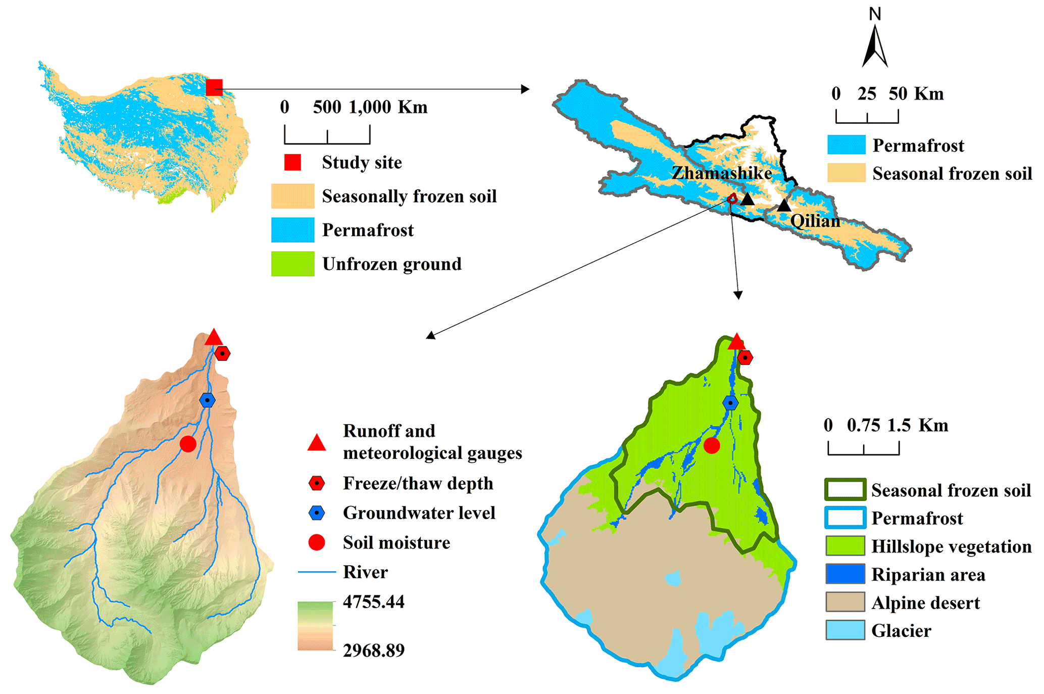
Figure 1Sketch map of the Qinghai–Tibet Plateau, with the distribution of permafrost and seasonal frozen soil of the QTP (Zou et al., 2014) and the location of the upper Heihe River basin (upper left). Sketch map of permafrost and seasonal frozen soil distribution of the upper Heihe River basin (Sheng, 2020) and the two subbasins, i.e., Zhamashike and Qilian, and the location of the Hulu catchment (upper right). Hulu catchment's digital elevation model (DEM), river channel, runoff, and meteorological gauge station (observed from 2011 to 2014), the locations for soil moisture (2011–2013 with data gap), groundwater level (2016–2019), and freeze/thaw depth (bottom left; 2011–2014). Landscapes and seasonal frozen soil/permafrost map of the Hulu catchment (bottom right).
The Hulu catchment mostly extends on seasonal frozen soil and permafrost (Zou et al., 2014; Ma et al., 2021). Field survey in the upper Heihe revealed that the lower limit of permafrost was 3650–3700 m (Wang et al., 2016); above that elevation is permafrost, and below is seasonal frozen soil. In the Hulu catchment, the lower limit of permafrost is around 3650 m (Fig. 1). Permafrost covers 64 % of the catchment area, and the seasonal frozen soil covers 36 %. There is a strong co-existence between soil freeze–thaw features and landscapes (Fig. 1). Permafrost and moraine/talus with poor vegetation cover co-exist at higher elevations, with large heat conductivity and less heat insulation in winter, resulting in a deep frozen depth. The seasonal frozen soil in relatively lower elevation has better vegetation cover, with better heat insulation and less heat conductivity in winter, resulting in a shallower frozen depth.
The elevation of the hydrometeorological gauging station is 2980 m. We collected daily runoff, daily average 2 m air temperature, and daily precipitation from 1 January 2011 to 31 December 2014. There was a flood event in 2013 which damaged the water level sensor and resulted in a runoff data gap from 17 June to 10 July in 2013. Soil moisture was measured in 20, 40, 80, 120, 180, 240, and 300 cm depths from 1 October 2011 to 31 December 2013, with a data gap between 3 August and 2 October 2012. In the same soil moisture site, we also observed the soil freeze/thaw depth from 2011 to 2014. Groundwater depth was measured at the WW01 site by four wells, with depths of 5, 10, 15, and 25 m, respectively (Pan et al., 2022). The observation period was from 2016 to 2019 and not overlaid with other hydrometeorological variables. Hence, we merely used the groundwater level to qualitatively constrain and test our perceptual model.
A perceptual model is increasingly recognized as being of central importance in hydrological model development (Savenije, 2009; Fenicia and McDonnell, 2022). Although the perceptual model is a qualitative representation of hydrological system, it bridges the gap between experimentalists and modelers and holds the base for a quantitative conceptual model. In this study, we developed a perceptual frozen soil hydrology model for the Hulu catchment, based on field measurements and our expertise.
3.1 Observation 1: low runoff in the early thawing season (LRET)
Precipitation–runoff time series analysis is a traditional and powerful tool to understand catchment hydrology. When we plot Hulu catchment's precipitation and runoff data together, we observed an interesting phenomenon, i.e., low runoff in the early thawing season (LRET; Fig. 3). For example, on 5–9 June 2013, there was a 45.7 mm rainfall event, with the air temperature ranging from 3.0 to 11.9 ∘C, but with only 0.68 mm in total runoff generation. Ma et al. (2021) also showed that, in the warm period in the middle of June 2015 in the Hulu catchment, there was a large rainfall event (over 30 mm d−1), but no runoff response was observed. Moreover, this LRET phenomenon happens every year, which allows us to exclude the possibility of measurement errors.

Figure 2Landscape classification at different elevation bands (with 50 m interval) of the Hulu catchment.
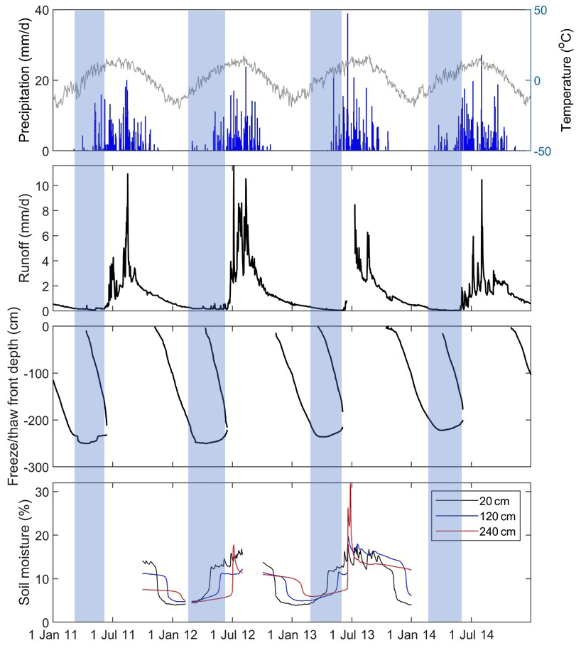
Figure 3Observed daily precipitation and air temperature, observed daily runoff depth of the Hulu catchment, observed freeze/thaw front depth, and observed soil moisture at depths of 20, 120, and 240 cm are shown.
To further investigate the LRET phenomenon, we plot the time series of observed daily precipitation, temperature, runoff, freeze/thaw front depth, and soil moisture profile (20, 120, and 240 cm) together (Fig. 3). Soil moisture data showed that topsoil was dry at the beginning of the thawing season. Gradually, soil was thawing from both topsoil and downwards (Fig. 3), and simultaneously, the soil moisture was increased also downwards. Although the topsoil was thawed, there was still frozen soil underneath (Fig. 3). The water above the frozen soil layer was even saturated with ponding, but there was no percolation and runoff generation. Moreover, the groundwater level further declined (Fig. 11). This illustrated that, during this period, the soil and groundwater system were disconnected, very likely because the frozen soil blocked the percolation. As revealed by isotope data in the Hulu catchment, groundwater contributed the dominant streamflow, i.e., 95 % during the frozen period (Ma et al., 2021). Thus, during this process, there was almost no runoff generation, and the only contribution to streamflow during this period was the discharge from groundwater system as baseflow. Our fieldwork experience also verified that, in the early thawing season, vehicles were easy to be trapped in mires because the surface soil was muddy, saturated, and even over-saturated with ponding. When frozen soil was completely thawed in summer, trafficability became much better.
When completely thawed, the bidirectional thaw fronts meeting the soil moisture in the bottom of frozen soil (around 2.4 m in this study site; Fig. 3) increased sharply and then decreased, with a short period pulse. We also noted that the observation sites of freeze/thaw front depth and soil moisture were both near the outlet of the Hulu catchment in lower elevation (Fig. 1). This means that, once the frozen soil in lower elevation was thawed, soil and groundwater systems were reconnected. Hydrological processes, including groundwater percolation and runoff generation, became the normal condition when they are free of frozen soil.
3.1.1 Learning from paired catchments
The LRET phenomenon was widely documented in other cold regions (Fig. 4), including, but not limited to, the headwater of Yellow River (Yang et al., 2019) and a small headwater catchment at the Cape Bounty Arctic Watershed Observatory, Melville Island, Nunavut, Canada (Lafrenière and Lamoureux, 2019). For example, at the headwater of Yellow River on 8–9 July 2014, there was a 21.9 mm rainfall event, with a temperature of 6.5 ∘C but little 1.5 m3 s−1 runoff. On 21–23 July 2014, there was a 27.4 mm rainfall event with temperature of 7.2 ∘C, but only 5.1 m3 s−1 runoff. Lafrenière and Lamoureux (2019) found that the undisturbed frozen soil at the Cape Bounty Arctic Watershed Observatory had little runoff generation in the early thawing season. But after the frozen soil was disturbed, the runoff response to rainfall event was much larger. Hence, this paired catchment study illustrated that frozen soil played a key role in causing the LRET phenomenon.
3.2 Observation 2: discontinuous baseflow recession (DBR)
Baseflow recession provides an important source of information to infer groundwater characteristics, including its storage properties, subsurface hydraulics, and concentration times (Brutsaert and Sugita, 2008; Fenicia et al., 2006), which is especially true for basins with frozen soil (Ye et al., 2009; Song et al., 2020).
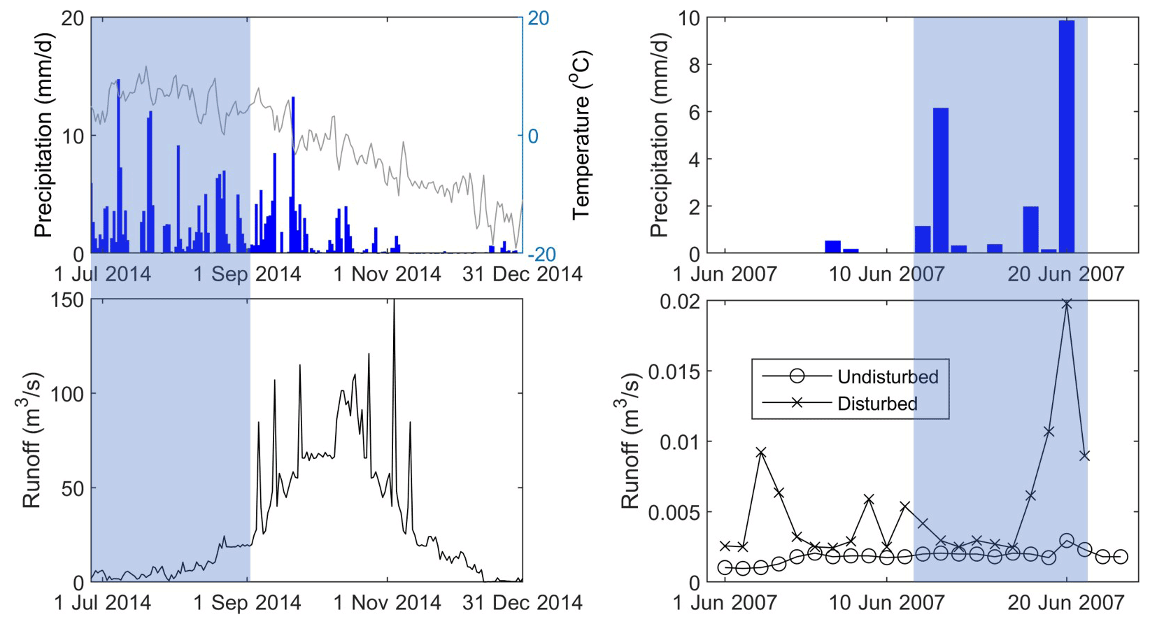
Figure 4The little runoff in the early thawing season (LRET) phenomenon in other places, e.g., the headwater of Yellow River (Yang et al., 2019) and a small headwater catchment at the Cape Bounty Arctic Watershed Observatory, Melville Island, Nunavut, Canada (Lafrenière and Lamoureux, 2019).
Baseflow analysis is based on the water balance equation (Eq. 1) and linear reservoir assumption (Eq. 2). It should be noted that Eq. (1) assumes no additional inflows (recharge or thawing) or outflow (capillary rise or freezing). If a reservoir is linear, then this implies that the reservoir discharge (Q) has a linear relationship with its storage (S). Ks (d) is a time constant controlling the speed of recession in the linear reservoir. With a larger Ks value, the reservoir empties slower and vice versa. Combining Eqs. (1) and (2), we can derive Eq. (3), illustrating how discharge depends on time (t), which is proportional to the initial discharge (Q0).
3.2.1 Baseflow recession analysis results
In Fig. 5, we plot the groundwater recession on semi-logarithmic scale. In the beginning of freezing season, baseflow presented a clear linear recession and was able to be fitted by setting the recession coefficient (Ks) as 80 d. However, interestingly, simultaneously with the LRET phenomenon, we observed a clear discontinuous baseflow recession in the Hulu catchment (Fig. 5). The baseflow bent down, and Ks became 60 d at the end of the recession period. This DBR phenomenon informed us that the groundwater system was disturbed. We also noted the spikes during the thawing in Fig. 5, which means that groundwater was suddenly released. To our best knowledge, these discontinuous baseflow recession (DBR) phenomena are a new observation for mountainous frozen soil hydrology.
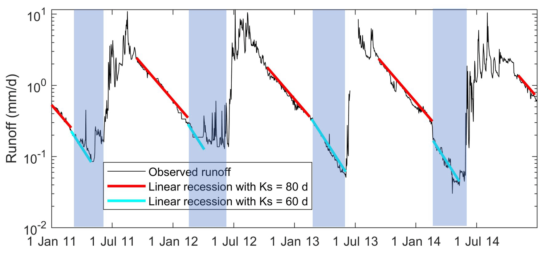
Figure 5Groundwater recession, from 2011 to 2014, on a logarithmic scale, with linear recession parameter Ks=80 d in the early recession periods and Ks=60 d at the end of the recession periods.
We also plot the variation in groundwater depth of four wells at the WW01 site from 2016 to 2019 (Figs. 1, 11). The wells of 5, 10, and 15 m only had liquid water in thawing seasons and gradually went dry in recession periods. The water level of the 25 m well was decreasing in the entire frozen seasons but in a discontinuous way. From the observed groundwater depth, the groundwater level decreases faster at beginning. And after the groundwater level dropped below around 17 m, the decrease in the groundwater level became slower. The turning point from Ks=80 d to Ks=60 d occurred simultaneously, while the groundwater level went down to 17 m (Figs. 5, 11). The bending down discontinuous baseflow recession and slower decrease of groundwater level indicated that there was a disturbance that reduced the groundwater discharge and lead to a slower decrease in the groundwater level.
3.2.2 Learning from paired catchments
Frozen soil process is able to disturb the groundwater system by freezing the liquid groundwater to reduce groundwater storage and leading to the DBR. But the DBR could also be caused by many other reasons, for instance soil evaporation, root tapping, capillary rise, impermeable layer, and heterogenous hydraulic conductivities in different landscapes (riparian area and hillslope). Since the DBR phenomenon started from the middle of the freezing period and lasted until the end of frozen season, in which time the evaporation, root tapping, and capillary rise were very inactive even totally stopped, this allowed us to exclude these impacts. The impermeable layer and heterogenous hydraulic conductivities are both able to result in discontinuous recession at the small scale.
To further understand the DBR phenomenon, we collected larger-scale runoff data in this region, including the Zhamashike (5526 km2) and Qilian (2924 km2), which are also the subbasins of the upper Heihe. The permafrost and seasonal frozen soil map of the upper Heihe River basin shows that the Zhamashike subbasin has 74 % permafrost and 26 % seasonal frozen soil, which is similar to the Hulu catchment while the Qilian subbasin has much less permafrost area (38 %) and is mostly covered by seasonal frozen soil (62 %; Fig. 1).
Interestingly, when plotting the hydrographs of these two subbasins on a logarithmic scale, we can clearly see that, in the permafrost-dominated Zhamashike subbasin, discontinuous recessions occurred, with Ks=60 d in the beginning and Ks=20 d at the end of the recession period. This DBR phenomenon is the same as found in the Hulu catchment, although the Zhamashike and Hulu catchment have quite different scales (5526 vs. 23.1 km2; Chen et al., 2018; Gao et al., 2014). Discontinuous baseflow recession happened almost every year at the Zhamashike station, and we only highlight the hydrograph in 1974 to demonstrate this phenomenon in Fig. 6. On the other hand, while being of similar size as the Zhamashike, the Qilian subbasin (2924 km2), which is mostly covered by seasonal frozen soil, only has one continuous recession, with Ks=60 d. The results from these two paired catchments provided good reasons to interpret the DBR phenomenon in the Hulu catchment as the result of frozen soil.
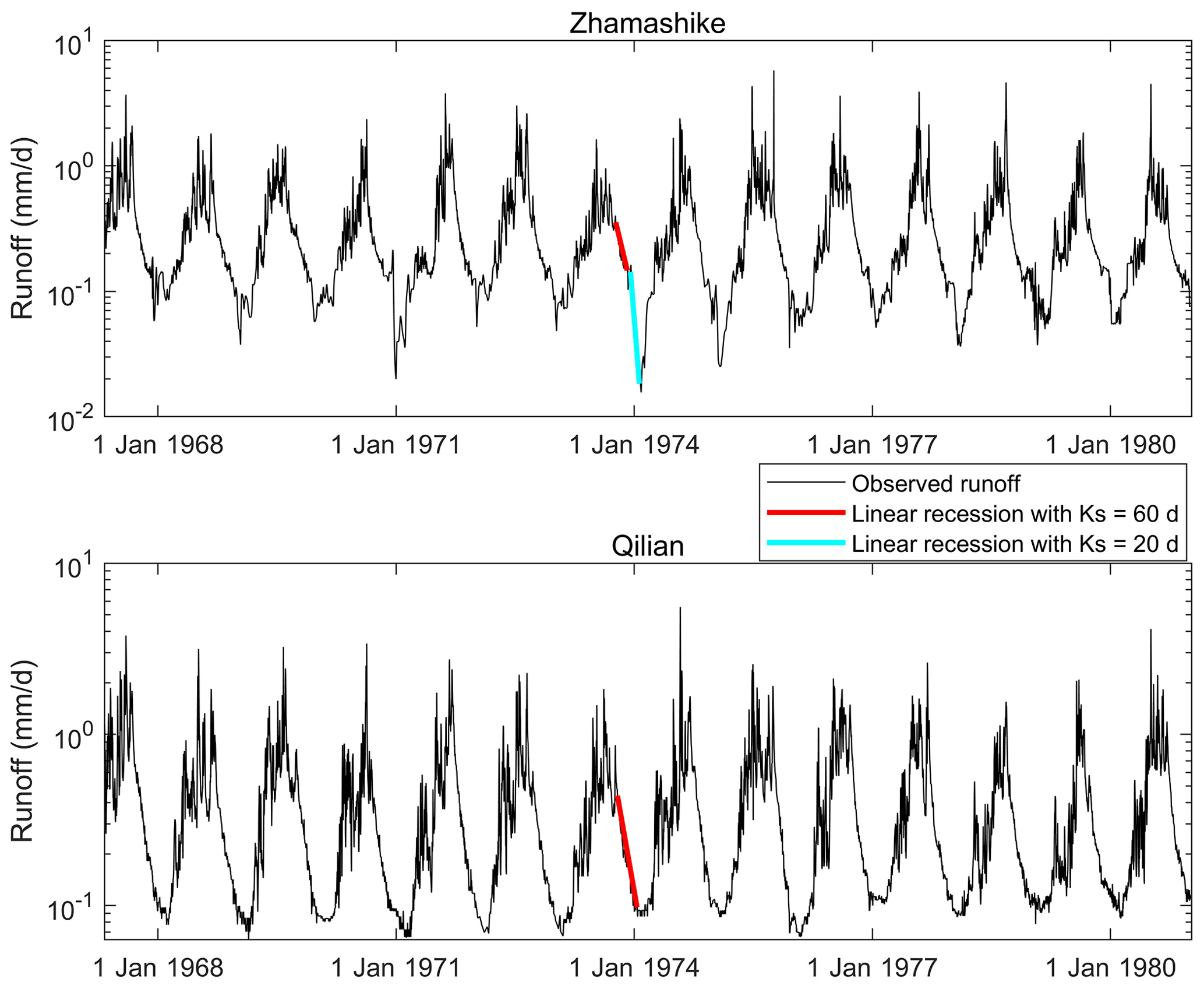
Figure 6The hydrograph of the Zhamashike and Qilian subbasin on logarithmic scale, and the linear recession curve with Ks=60 d and Ks=20 d.
3.3 Perceptual frozen soil hydrology model of Hulu catchment
We did an expert-driven data analysis of the LRET and DBR observations, including a time series analysis of precipitation–runoff, soil moisture profile, freeze/thaw depth, and paired catchments comparison. These comprehensive data analyses allowed us to identify that both the LRET and the DBR were the results of frozen soil, and these results motivated the following perceptual model (Fig. 7).
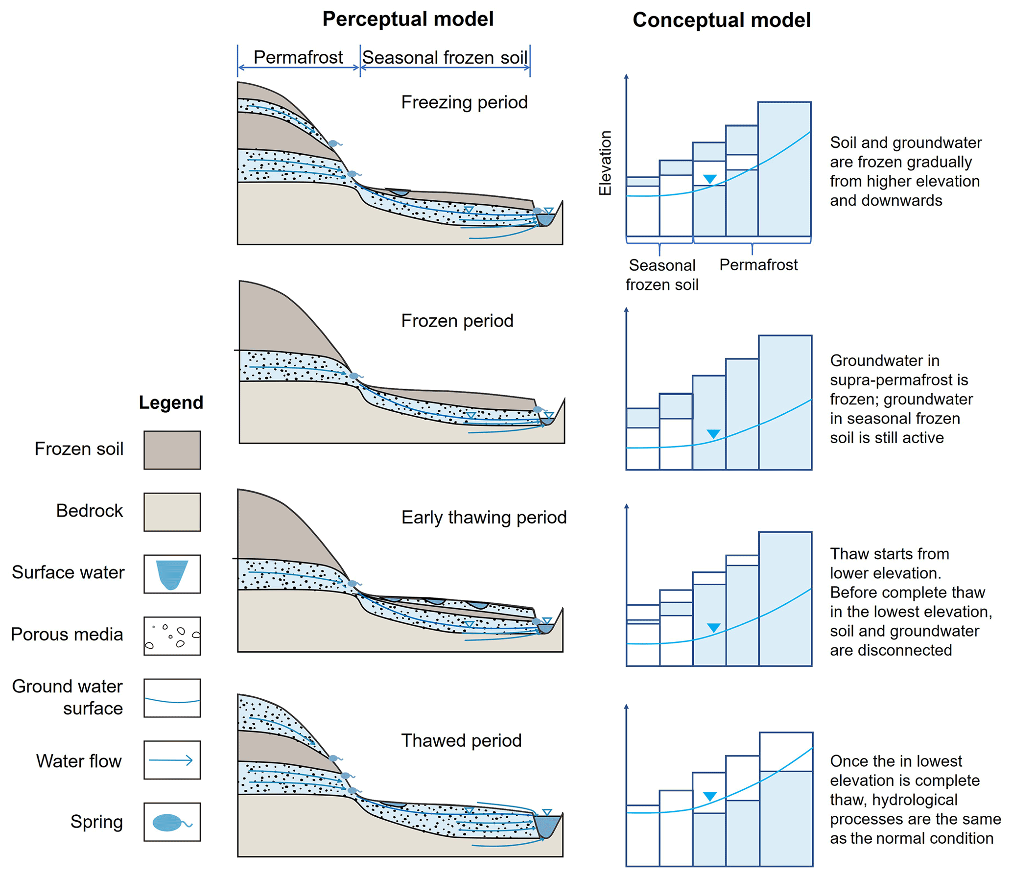
In the freezing season, at local scale, frozen soil occurs from the topsoil downwards. But at the catchment scale, the freezing process does not occur in a homogeneous way. Since the higher elevation is colder than the lower elevation, the freezing process starts from higher elevation and moves downwards. At the beginning of the freezing season, although the topsoil is already frozen, the groundwater discharge from the supra-permafrost layer still continues. It was found that the groundwater recession from the supra-permafrost layer determines the dominant part of baseflow in permafrost regions (Brutsaert and Sugita, 2008; Ma et al., 2021). Thus, the baseflow recession contributed by both permafrost and seasonal frozen soil areas, during this period, appears not to be influenced by frozen topsoil and maintains a linear recession pattern, with Ks=80 d in the Hulu catchment.
In the frozen season, the hydrological processes in the topsoil are almost completely blocked, although there is still very small amount of unfrozen liquid water in the frozen soil. Thus, surface hydrological processes are almost stopped. With the increase in frozen depth, groundwater in the supra-permafrost layer is frozen gradually from higher to lower elevation, which gradually but dramatically reduces groundwater discharge. Interestingly, permafrost and seasonal frozen soil have different impacts on baseflow recession. In a seasonal frozen soil region, with shallower frozen depth, the groundwater is still active and continues the discharge. But in the permafrost region, the groundwater in the supra-permafrost layer is largely inactive. This means that the recession, in the frozen periods, was only contributed by the seasonal frozen soil area, with a faster decline in baseflow and bending down of the hydrograph, with Ks decreasing to 60 d in the Hulu catchment.
During the early thawing season, after a long groundwater recession, the groundwater level is deep. Due to soil evaporation in winter, the soil is dry and has a moisture deficit. Observations show that, with the progression of thawing, soil temperature and soil moisture increase from top to bottom, and the thawing front deepens downward. Rainfall firstly infiltrates to saturate the moisture deficit without runoff generation. Moreover, the existence of the impermeable deeper frozen soil layer leads to a vertical disconnection between soil water and groundwater. Although there is probably saturated water above the frozen soil (Figs. 3 and 7), the poor vertical connectivity largely hinders soil water percolation. Without recharge to groundwater, there is limited runoff generation during the early thawing.
At the end of the thawing season, as soon as the thaw depth reaches its maximum, or frozen soil no longer exists, the frozen groundwater is released. The spikes in the observed hydrograph are likely due to different parts of the catchment reaching a breakthrough, which happens first in the lower elevations and then gradually moves upward to higher landscape elements. This would trigger a sequence of sudden groundwater release and the spikes. Snowfall is probably another influencing factor that causes the LRET and the spikes phenomenon by storing precipitation as snow cover to reduce runoff and releasing melting water in a short time. This hypothesis needs to be tested by including snow accumulation and melting processes in the hydrological model.
Once the soil is completely thawed at the end of the melting season, the rainfall–runoff process returns to normal and is free of influence by the frozen soil. Hence, in the Hulu catchment, frozen soil mainly impacts on streamflow during the freezing, frozen, and thawing periods.
Based on this perceptual model, we developed the conceptual framework of the frozen soil hydrological model, which needs to at least to consider the following elements: (1) we need a semi-distributed modeling framework, (2) a distributed forcing should be considered, (3) different landscapes should be included, (4) topography should be involved, particularly elevation, (5) we need to consider soil freeze–thaw processes, (6) snowfall and melting should be included, (7) glacier melting should be included, and (8) last, but not least, the normal rainfall–runoff processes are still important because most runoff happens in the warm season, which functions in the same way as in temperate climate regions.
The perceptual model requires a quantitative conceptual model to test, revise, polish, verify, or even reject its hypotheses. Since the Hulu catchment has heterogenous landscapes with a large elevation gradient, diverse land cover, and complex freeze–thaw process, we developed a semi-distributed frozen soil hydrological model, i.e., FLEX-Topo-FS, based on the landscape-based hydrological modeling framework, i.e., FLEX-Topo. Numerous processes were involved in FLEX-Topo, including the distributed meteorological forcing, landscape heterogeneity, and snow and glacier melting. And in FLEX-Topo-FS, we explicitly considered the impacts of frozen soil on soil water percolation and groundwater frozen processes in the supra-permafrost layer. The details of both the FLEX-Topo model (without frozen soil) and FLEX-Topo-FS model (with frozen soil) are described in below.
4.1 FLEX-Topo model (without frozen soil)
4.1.1 Catchment discretization and meteorological forcing interpolation
The FLEX-Topo model classified the entire Hulu catchment into four landscapes, i.e., glaciers, alpine desert, vegetation hillslope, and riparian zone. The Hulu catchment (from 2960 to 4820 m) was classified into 37 elevation bands, with 50 m intervals (Fig. 2). Combining the four landscapes and 37 elevation bands, we had 37 × 4 = 148 hydrological response units (HRUs). The structure of FLEX-Topo model consisted of four parallel components representing the distinct hydrological function of different landscape elements (Savenije, 2010; Gao et al., 2014; Gharari et al., 2014; Gao et al., 2016). And the corresponding discharge of all elements was subsequently aggregated to obtain the simulated runoff.
We interpolated the precipitation (P) and temperature (T) based on elevation bands from in situ observation (2980 m) to each elevation band. The precipitation increasing rate was set as 4.2 %/100 m and the temperature lapse rate as −0.68 ∘C/100 m, based on field measurements (Han et al., 2013). Snowfall (Ps) or rainfall (Pl) was separated by air temperature, with the threshold temperature as 0 ∘C (Gao et al., 2020).
4.1.2 Model description and configuration
FLEX-Topo is a semi-distributed conceptual bucket model (Savenije, 2010; Gao et al., 2014), with three modules, i.e., the snow and glacier module, the rainfall–runoff module, and the groundwater module. The water balance and constitutive equations can be found in Table 1. The model parameters and their prior ranges for calibration are listed in Table 2.
Table 1The water balance and constitutive equations used in FLEX-Topo-FS model. In Eqs. (10), (11), and (12), the Su and Sumax represent root zone reservoirs and their storage capacities in different landscapes, including vegetation hillslope (Sumax_V), alpine desert (Sumax_D), and riparian regions (Sumax_R).
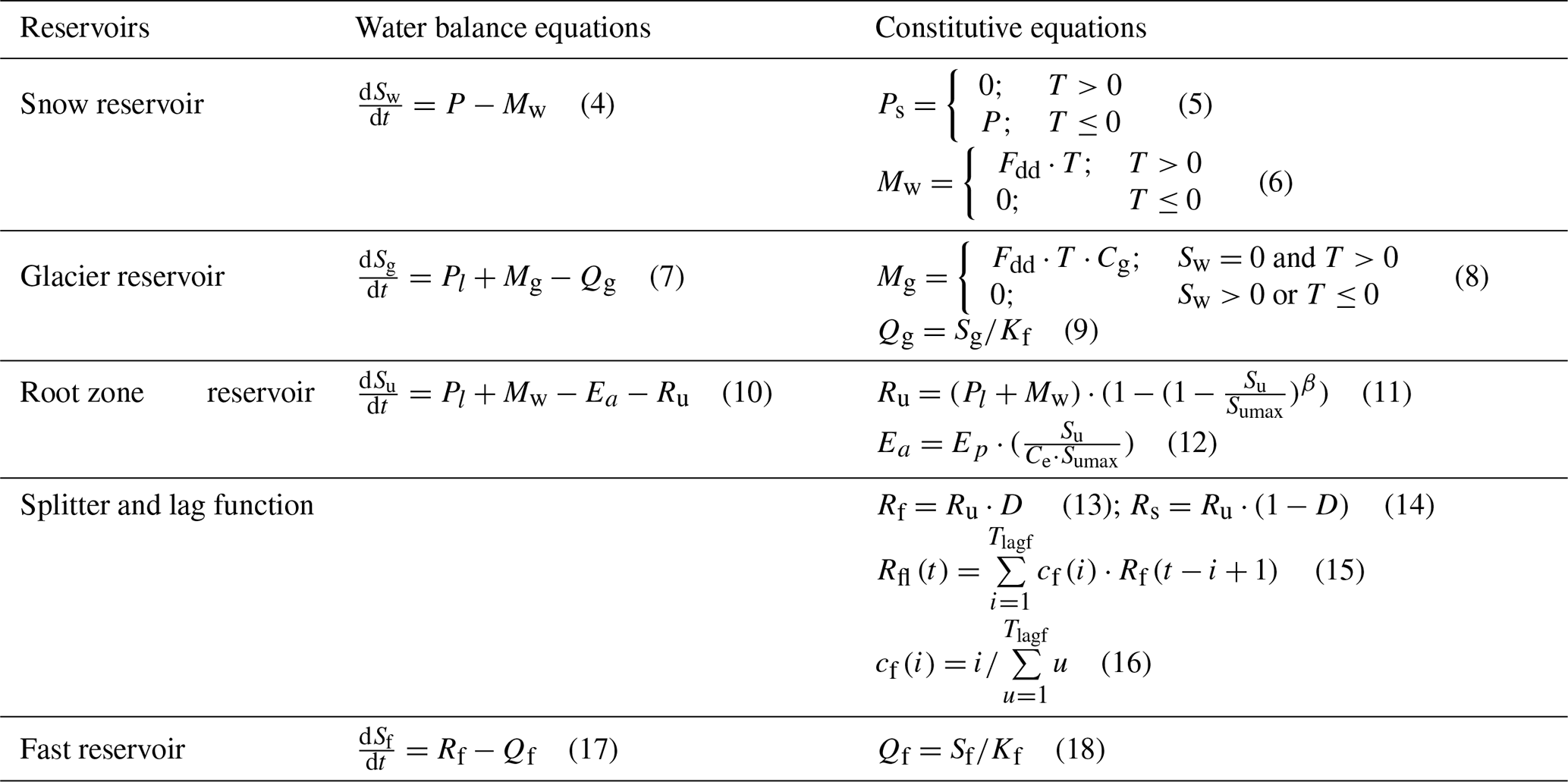
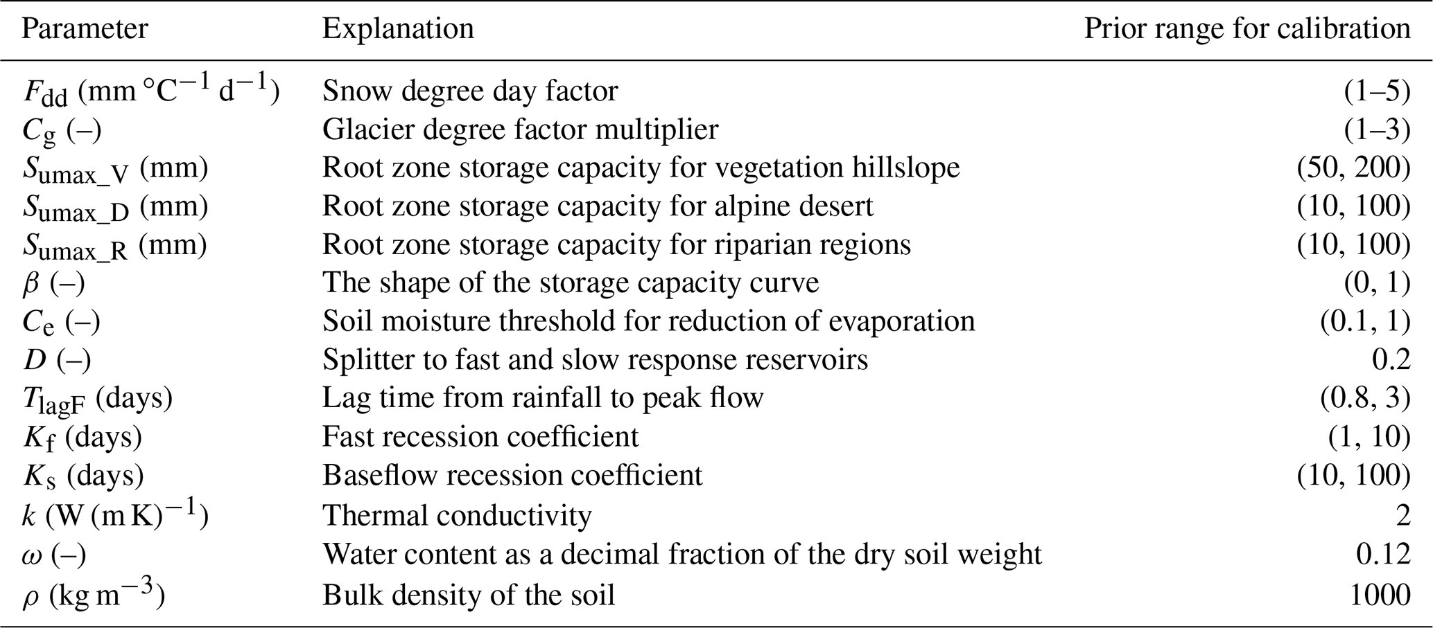
Table 2The parameters of the FLEX-Topo-FS model and their prior ranges for calibration.
Snow and glacier module
The temperature index method was employed to simulate snow and glacier melting (Gao et al., 2017, 2020; He et al., 2021). We used a snow reservoir (Sw) to account for the snow accumulating, melting (Mw), and water balance (Eq. 4). The snow degree day factor (Fdd) needs to be calibrated. For glaciers, we assumed its area was constant in our simulation (from 2011 to 2014). Glacier melting (Mg) was also calculated by the temperature index method (Eq. 7) but with a different degree day factor. With the same air temperature, the glacier has less albedo than snow cover, thus with a larger amount of melting. The glacier degree factor was obtained by multiplying the snow degree day factor (Fdd) with a correct factor Cg (Eq. 8; Gao et al., 2020).
Rainfall–runoff module
There are two reservoirs to simulate rainfall–runoff process, including the root zone reservoir (Su; Eq. 10) and fast response reservoir (Sf; Eq. 17). To account for the different rainfall–runoff processes in different landscapes and simultaneously avoid over-parameterization, we kept the same model structure for vegetation hillslope, riparian zone, and alpine desert (Eqs. 11, 12) but gave different root zone storage capacity (Sumax) values, i.e., Sumax_R for riparian zone, Sumax_D for cold desert, and Sumax_V for hillslope vegetation. For vegetation hillslope, a larger prior range was constrained for the root zone storage capacity (Sumax_V), which means more water is required to fill in its storage capacity to meet its water deficit, which is evidenced by previous studies in this region (Gao et al., 2014). For alpine desert, due to its sparse vegetation cover, we constrained a shallower root zone storage capacity (Sumax_D). For the riparian area, due to the location where is prone to be saturated, we also constrained a shallower root zone storage capacity (Sumax_R). The initial states (beginning of 2011) of the reservoirs were obtained from the end values (end of 2014) of the simulation, which is a normal procedure in modeling practice.
Other parameters in the rainfall–runoff module (Eqs. 11–18; Table 1) include the threshold value controlling evaporation (Ce), the shape parameter of the root zone reservoir (β), the splitter (D) separating the generated runoff (Ru) from the root zone reservoir (Su) to the fast response reservoir, the recession parameter of faster reservoir (Kf), and the lag time from rainfall event to peak flow (TlagF). We set D as 0.2 from the isotope study (Ma et al., 2021) and other parameters were calibrated, with prior ranges (Table 2) based on previous studies (Gao et al., 2014, 2020).
Groundwater module
The baseflow (Qs) is generated from groundwater recession. The groundwater was simulated by a linear reservoir (Ss), described in Sect. 3.2 and Eq. (19). We set the prior range for s recession coefficient of the baseflow reservoir (Ks) as 10–100 d. To estimate the impacts of frozen groundwater on hydrological processes, we set the groundwater in different landscapes as parallel. But we analyzed the groundwater level as an integrated system because the groundwater system is connected, and this affects the groundwater level. Since the subpermafrost groundwater is even deeper than 20 m in the Hulu catchment and almost disconnected to streamflow, we only model the supra-permafrost groundwater.
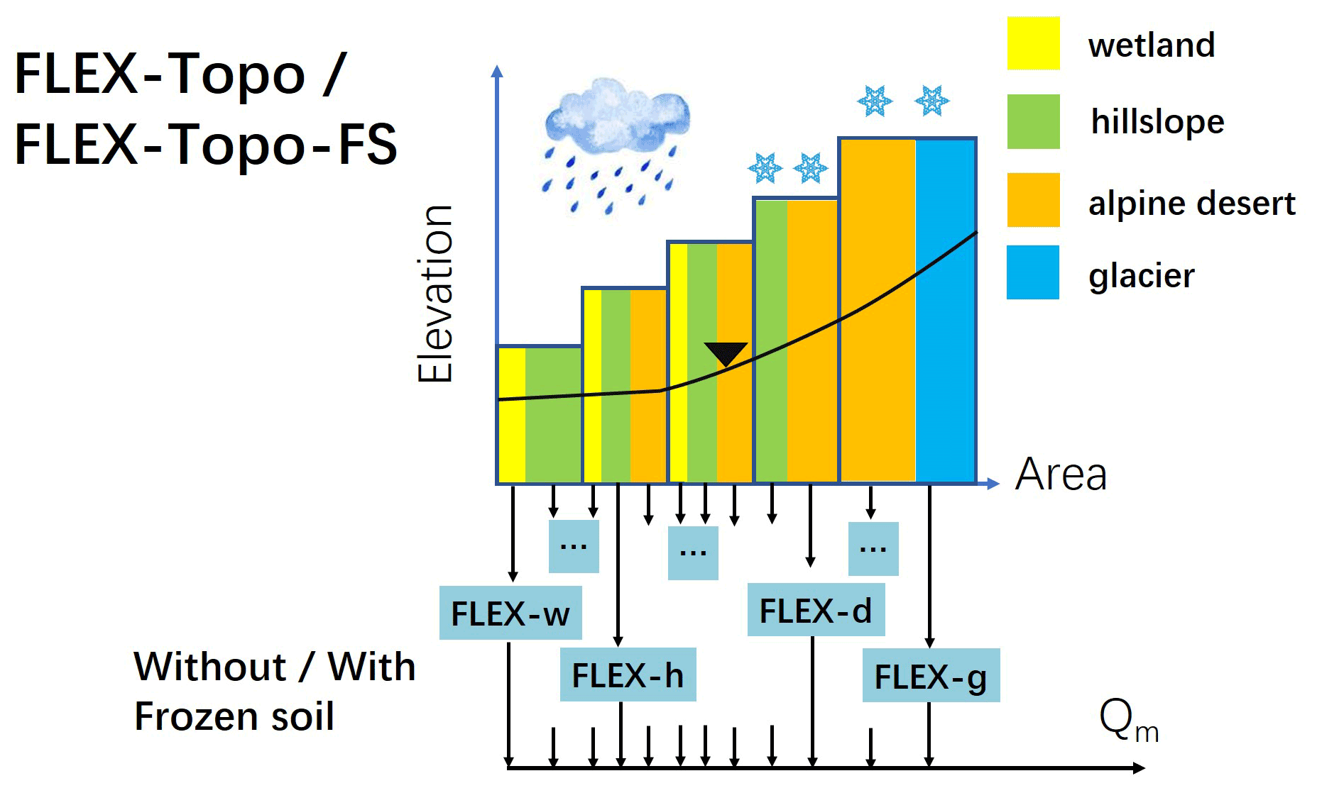
Figure 8Model structures of FLEX-Topo and FLEX-Topo-FS. FLEX-w means the module for wetland, FLEX-h for hillslope, FLEX-d for alpine desert, and FLEX-g for glacier, respectively.
4.2 FLEX-Topo-FS model (with frozen soil)
4.2.1 Modeling the soil freeze–thaw processes
The FLEX-Topo-FS model employed the Stefan equation (Eq. 20) to provide an approximate solution to estimate freeze/thaw depth (Fig. 9). The Stefan equation is a temperature-index-based freeze–thaw algorithm which assumes the sensible heat is negligible in soil freeze–thaw simulation (Xie and Gough, 2013). The form of Stefan equation is written as follows:
where ε is the freeze/thaw depth, k is the thermal conductivity (W (m K)−1) of the soil, and F is the surface freeze–thaw index. The freeze index (∘ of degree days) is the accumulated negative ground temperature while freezing, and the thaw index (∘ of degree days) is the accumulated positive ground temperature while thawing. QL (J m−3) is the volumetric latent heat of soil. , where L is the latent heat of the fusion of ice (3.35×10⁵ J kg−1). ω is the water content, as a decimal fraction of the dry soil weight, and ρ is the bulk density of the soil (kg m−3).

We set the thermal conductivity as k=2 W (m K)−1, the water content as a decimal fraction of the dry soil weight ω=0.12, and the bulk density of the soil as ρ=1000 kg m−3. Since the Stefan equation requires ground surface temperature, which is difficult to measure and often lacks data, we used a multiplier to translate the air temperature to ground temperature. The multiplier during freezing was set as 0.6, and during thawing, we assumed the ground surface temperature was the same as the air temperature (Gisnås et al., 2016).
In this model, we did not consider the impacts of snow cover on soil freeze–thaw because the snow effects were complicated in the Hulu catchment. First, this is because precipitation in the Hulu catchment mostly happens in summer as rainfall, and snow depth in the Hulu catchment was less than 10 mm in most areas most of the time. Second, the snow cover has contrary effects on ground temperature. Snow cover as an isolation layer increased ground temperature in winter. But, simultaneously, snow cover also increased albedo, which decreased the net radiation and decreased ground temperature. To avoid over-parameterization, we did not consider snow effect in the Stefan equation.
In this study, the Stefan equation was driven by distributed air temperature, which allowed us to simulate the distributed soil freeze–thaw processes. With the distributed soil freeze index and thaw index, we can also estimate the lower limit of permafrost at which elevation the freeze index equals the thaw index in mountainous regions. Field surveys on the lower limit of permafrost (Wang et al., 2016) can provide another strong confirmation of our simulated soil freeze–thaw process, except for the spot-scale freeze/thaw depth.
4.2.2 Modeling the impacts of frozen soil on hydrology
The distributed freeze–thaw status calculated by the FLEX-Topo-FS model allowed us to simulate the impacts of frozen soil on soil and groundwater systems, their connectivity, and, eventually, catchment runoff.
In freezing and frozen seasons, precipitation was in the phase of snowfall, and topsoil was frozen, thus without surface runoff. During this period, runoff is only contributed from the groundwater discharge of the supra-permafrost layer (Qs). There is no runoff generation (Ru) from the root zone reservoir to the response routine (Ss and Sf) in this period. In the conceptual model, we set Ru=0 (Eq. 11). In freezing season, when frozen depth was less than 3 m (the depth of active layer in this region), the entire groundwater volume in the supra-permafrost layer was still connected and could be simulated by linear groundwater reservoir (Ss). Once the frozen depth of certain elevation zone is larger than 3 m, the groundwater in that elevation zone was frozen (Fs). In the FLEX-Topo-FS model, we reduced the groundwater storage (Ss) to 10 % of its total storage to simulate its frozen status (Eqs. 21, 22). This amount of frozen water (Fs, 90 % of groundwater storage when frozen and marked as was held in the groundwater system as frozen soil (Eq. 22) but did not disappear. We set 90 % as frozen, rather than 100 %, because there is still unfrozen liquid water in frozen soil (Romanovsky and Osterkamp, 2000). Groundwater discharge was controlled by the frozen status, which was frozen from high elevations to lower elevations. This process is progressively stopping the function of a series of cascade groundwater buckets, resulting in the discontinuous recession. Simultaneously, the decrease in discharge (Qs) slowed down the decrease in the groundwater level (Ss). This conceptual model allowed us to simulate the bending down of baseflow recession and slower decrease in groundwater level.
In thawing seasons, the freeze–thaw condition in the lowest elevation zone plays a key role, controlling the hydraulic connectivity between soil and groundwater systems. In the conceptual model, if the freeze depth calculated by the Stefan equation is larger than the thaw depth, then this means that the frozen layer still exists, which obstructs the soil and groundwater connection. In the conceptual model, we kept Ru=0 (Eq. 11) as the runoff generation. Since there is no percolation from soil to groundwater, root zone soil moisture (Su) is accumulating and even ponding in some local depressions (Fig. 7). The only outflow of the root zone is evaporation in this period. This conceptual model allowed us to reproduce the LRET observation. For groundwater reservoir, once the thaw depth goes to its yearly maximum (in permafrost area) or thaw depth > freeze depth (in seasonal frozen soil area), the frozen water (90 % of groundwater storage when frozen; was released to the groundwater again (Eq. 22). The sudden release of frozen groundwater causes the spikes in hydrograph, which could happen in either thawing seasons or complete thaw seasons, depending on its elevation. But either way, the water balance calculation is 100 % closed.
Complete thaw in the lowest elevation marked the end of thawing season and the start of complete thaw season. In the complete thaw season, soil water and groundwater are connected, and runoff generation (Ru) returns to normal circumstances, which can be simulated by the FLEX-Topo model without frozen soil.
4.3 Model uncertainty analysis and evaluation metrics
The Kling–Gupta efficiency (KGE; Gupta et al., 2009) was used as the performance metric in model calibration, as follows:
where r is the linear correlation coefficient between simulation and observation. α () is a measure of relative variability in the simulated and observed values, where σm is the standard deviation of simulated variables, and σo is the standard deviation of observed variables. β is the ratio between the average value of simulated and observed variables.
We applied the Generalized Likelihood Uncertainty Estimation framework (GLUE; Beven and Binley, 1992) to estimate model parameter uncertainty. We sampled the parameter space with 20 000 parameter sets and selected the top 1 % parameter as behavioral parameter sets.
For a comprehensive assessment of model performance in validation (Zhang et al., 2018), the behavioral model runs were evaluated using multiple criteria, including KGE, KGL (the KGE of the logarithms' flow and more sensitive to baseflow), Nash–Sutcliffe efficiency (NSE; Nash and Sutcliffe, 1970; Eq. 24), coefficient of determination (R2), and root mean square error (RMSE).
where Qo is observed runoff, is the observed average runoff, and Qm is modeled runoff.
The model was calibrated in the period 2011–2012 and uses KGE as the objective function. The second half of the time series (2013–2014) was used to quantify the model performance in streamflow split-sample validation, with multi-criteria including KGE, KGL, NSE, R2, and RMSE. The KGE, KGL, NSE and R2 are all less than 1, and their valuation closer to 1 indicates better model performance, while the lower value of RMSE indicates less error and better performance.
5.1 FLEX-Topo model results and its discrepancy
Figure 10 shows that the FLEX-Topo model can somehow reproduce the observed hydrography in most periods, except for the LRET and DBR events. In the calibration, the KGE was 0.78. And in the validation, KGE = 0.58, KGL = 0.36, NSE = 0.41, R2=0.82, and RMSE = 0.95 mm d−1. While taking account the impacts of landscape heterogeneity, the FLEX-Topo model can, to some extent, simulate the LRET phenomenon. The vegetated hillslope in relatively lower elevation has larger unsaturated storage capacity, with larger soil moisture deficit in the beginning of melting season, and is capable of holding more rainfall with initial dry soil. Moreover, FLEX-Topo model has taken snow accumulation and melting into account, which also reduced the runoff generation during the LRET periods. However, there was still large overestimation in the early thawing season.
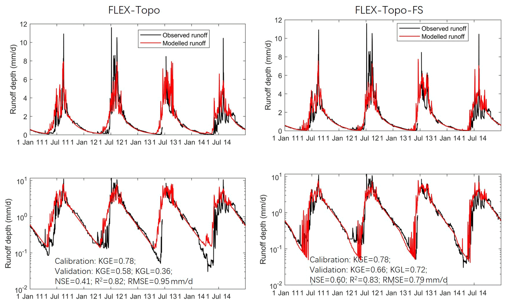
Figure 10Modeling results of FLEX-Topo and FLEX-Topo-FS models and the comparisons with observation on both normal and logarithmic scales.
Additionally, the simulated hydrography on the logarithm scale clearly shows that the baseflow is the result of a linear reservoir (Fig. 10). The linear reservoir model can mimic recession quite well at the beginning of a baseflow recession, but the model discrepancy becomes larger in the middle to the end of frozen season. Hence, the FLEX-Topo model is not able to simulate the discontinuous recession. The model discrepancy indicates that, without considering frozen soil, FLEX-Topo cannot reproduce the observed LRET and DBR observations well, although it explicitly considered landscape heterogeneity, snow, and glacier processes.
5.2 FLEX-Topo-FS model results
5.2.1 Freeze–thaw simulation by FLEX-Topo-FS model
Figure 9 demonstrates that the Stefan equation was capable to reproduce the freeze–thaw process. This verified the success of the freeze–thaw parameterization and the parameter sets. Also, the simulated lower limit of permafrost is 3716 m, which is largely close to the field survey in the upper Heihe River basin, at around 3650–3700 m (Wang et al., 2016), and the expert-based estimation of 3650 m of the Hulu catchment. Both the well reproduced freeze–thaw variation in the spot scale and the lower limit of permafrost in the catchment scale gave us strong confidence in the simulation of soil freeze–thaw processes.
5.2.2 Runoff simulation by FLEX-Topo-FS model
While considering the impacts of frozen soil, the FLEX-Topo-FS model, compared with FLEX-Topo, dramatically improved the model performance. Figure 10 shows the simulated hydrograph by FLEX-Topo-FS on both normal and log scales. Both the LRET and the DBR observations were almost perfectly reproduced by the FLEX-Topo-FS model. The KGE of FLEX-Topo-FS in calibration was 0.78, which was the same as FLEX-Topo. But in validation, the performance was significantly improved; the KGE improved from 0.58 to 0.66, KGL from 0.36 to 0.72, NSE from 0.41 to 0.60, R2 from 0.82 to 0.83, and RMSE reduced from 0.95 to 0.79 mm d−1. All the model evaluation criteria were improved. The most significant improvement was the baseflow simulation, and KGL was increased from 0.36 to 0.72. We also noted that the FLEX-Topo-FS model reproduced the spikes during the thawing in Fig. 10. This further confirms our conceptual model of a sequence of thawing breakthroughs, which triggers the sudden release of groundwater starting at lower elevations and progressing to higher landscape elements.
5.2.3 Modeling groundwater trends
To further verify the FLEX-Topo-FS model, we averaged the simulated groundwater storage (Ss) of all HRUs and compared this with the observed groundwater depth on the log scale (Fig. 11). We included the frozen groundwater in the total groundwater storage (Ss) because the liquid groundwater is in connection with the frozen groundwater, and this affects the groundwater level variation. Figure 11 clearly demonstrates that the simulated groundwater storage decreased slower, and the timescale of the recession increased. The trends of simulated groundwater storage and observed groundwater level, which are not the same but have a similar physical meaning describing the groundwater dynamic, correspond surprisingly well. This is particularly encouraging, given that the periods of simulation (2011–2014) and observation (2016–2019) were not overlaid, and a point observation may not be straightforwardly representative for the entire basin.
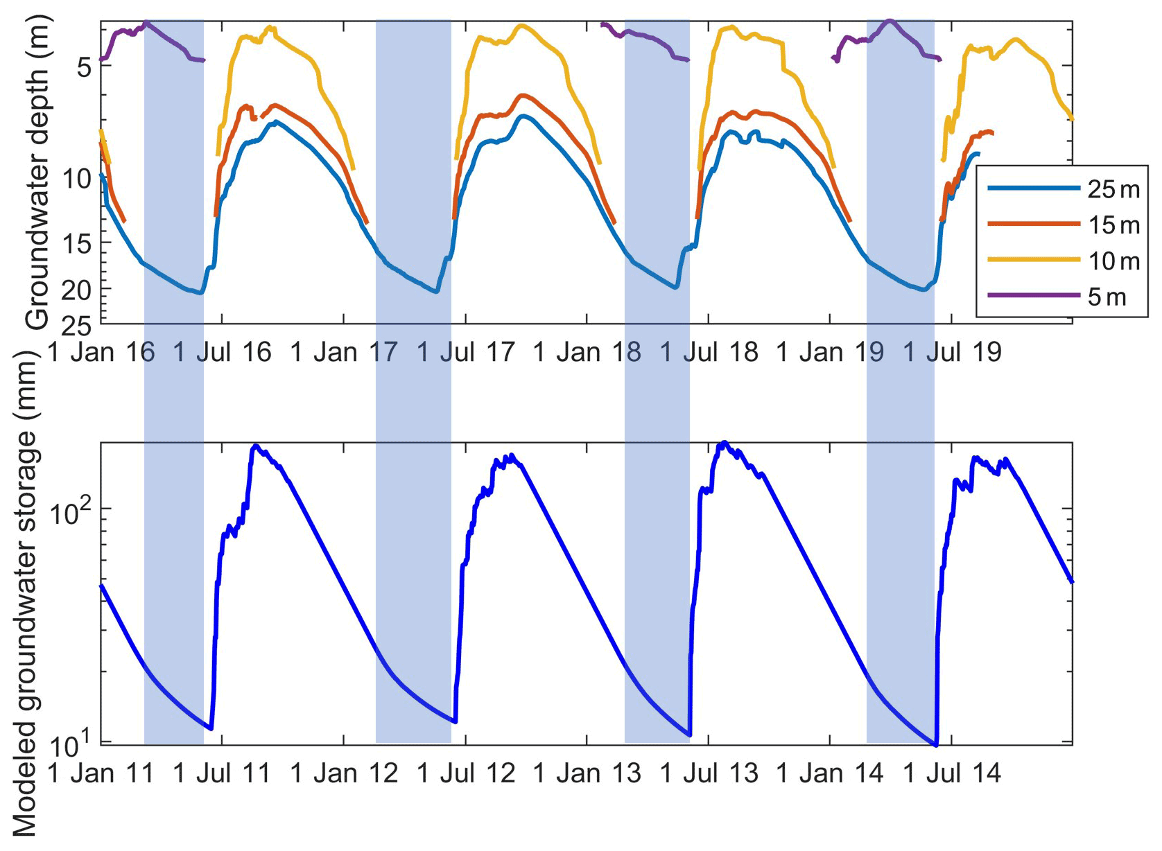
Figure 11Observed groundwater depth from 2016 to 2019 at WW01 wells, at depths of 5, 10, 15, and 25 m, and the simulated groundwater storage by the FLEX-Topo-FS model from 2011 to 2014.
The success in reproducing groundwater level trends is another strong confirmation for the FLEX-Topo-FS model. All the successes of the FLEX-Topo-FS model in reproducing spot-scale freeze/thaw depth variations lower the limit of permafrost, LRET and DBR events, and groundwater level trends, giving us strong confidence in the realism of our qualitative perceptual model and quantitative conceptual model.
6.1 Diagnosing the impacts of frozen soil on complex mountainous hydrology
6.1.1 Understanding complex frozen soil hydrology by hydrography analysis
Frozen soil happens underneath the ground, with frustrating spatiotemporal heterogeneities, and is difficulty to measure. Although there are spot and hillslope measurements, its impact on catchment hydrology is still hard to explore. Hydrography, easily and widely observed and globally accessible, can be regarded as the by-product of the entire catchment hydrological system (Gao, 2015). Hydrography as an integrated signal provides us with a vital source of information, reflecting how the complex hydrological system works, i.e., transforming precipitation into runoff. Hence, hydrography itself is a valuable source of data for understanding catchment frozen soil hydrology. Especially the baseflow embodies the influence of basin characteristics, including the geology, soils, morphology, vegetation, and frozen soil (Blume et al., 2007; Ye et al., 2009). Hence, a quantitative description of baseflow is a valuable tool for understanding how the groundwater system behaves (McNamara et al., 1998). Baseflow recession was used to identify the impacts of climate change on permafrost hydrology. In previous studies, Slaughter and Kane (1979) found that basins with permafrost have higher peak flows and lower baseflows. The baseflow, representing groundwater recession, provides important information about the storage capacity and recession characteristics of the active layer in permafrost regions (Brutsaert and Hiyama, 2012).
Moreover, the hydrological system has tremendous influencing factors. The hydrograph of paired catchments provides a good reference, as a controlled experiment, to isolate one influencing factor from the others. Nested catchments help us to acknowledge the importance of region-specific knowledge, which is often the key to interpreting the unexplained variability in large sample studies (Fenicia and McDonnell, 2022). In this study, the pair catchment method helped us to confirm the impacts of frozen soil on LRET and DBR observations.
Additionally, by analyzing the nested subbasins of the Lena river in Siberia, Ye et al. (2008) used the peak flowbaseflow ratio to quantify the impact of permafrost coverage on hydrograph regime in the Lena river basin and found that frozen soil only affects the discharge regime over high permafrost regions (greater than 60 %) and has no significant affect over the low permafrost (less than 40 %) regions. In this study, we reconfirmed this statement. The permafrost area proportions of the Hulu catchment and Zhamashike subbasin are 64 % and 74 %, with significant effects on discharge, while 38 % of the Qilian subbasin is covered by permafrost, with no significant effects on discharge regime.
By using the paired catchments comparison, interestingly, the Ks in Zhamashike and Qilian in the early recession period are both 60 d, which is exactly within the standard value of 45 ± 15 d derived in earlier studies for basins ranging in size between 1000 and 100 000 km2 (Brutsaert and Sugita, 2008; Brutsaert and Hiyama, 2012), which was likely the results of catchment self-similarity and co-evolution. But we also noticed that the Ks in the small Hulu catchment (Ks=80 and 60 d) is quite a bit larger than the Zhamashike (Ks=60 and 20 d) and Qilian (Ks=60 d). This could be rooted in different scale and drainage density (Brutsaert and Hiyama, 2012). The Hulu catchment is located in the headwater with less drainage density; hence, there is less contact area between the hillslope and river channel, a slower baseflow recession, and a larger Ks value. We argue that, even without the impacts from frozen soil, it is difficult to give accurate Ks estimation in small catchments (less than 1000 km2) in moderate climates. It is more substantially difficult to estimate the discontinuous Ks in different periods in frozen soil catchments without calibration. Thus, estimating the value of recession coefficient (Ks) in different catchments and periods, especially for small catchments and in cold regions, is still an intriguing scientific question for hydrologists.
6.1.2 Understanding complex frozen soil hydrology by multi-source observations
Observation is still a bottleneck in complex mountainous cold regions. Traditionally, fragmented observations are only for specific variables, like puzzles. In this study, we collected multi-source data, including soil moisture, groundwater level, topography, geology survey, isotope, soil temperature, freeze/thaw depth, permafrost and seasonal frozen soil maps, and hydrographs in paired catchments. Multi-source data analysis provides a multi-dimensional perspective to investigate frozen soil hydrology. We argue that, on the one hand, multi-source observations helped us to deliver the perceptual and conceptual models. And on the other hand, perceptual and conceptual models bridge the gap between experimentalists and modelers (Seibert and McDonnell, 2002), allowing us put fragmented observations together and understand the hydrological system in an integrated and qualitative way.
The data gap is a common issue in mountainous hydrology studies. For example, in this study, runoff data have a gap period at the end of the thawing season in 2013 due to flooding and equipment malfunction. Soil moisture and groundwater level data had large gap, which cannot be used for continuous modeling. Luckily, the meteorological data, which are important forcing data for running the models, were continuous and without any gap. With sufficient meteorological forcing data, we successfully run the hydrological models from 2011 to 2014. The runoff data gap at the end of thawing season in 2013 merely influenced model validation. While evaluating the models, we did not involve the data gap period. Hence, the data gap does not have any impact on the consolidation of the conclusions.
Although soil moisture had large gap, there were, fortunately, some observations during the LRET periods, which were sufficient to distinguish the impacts of frozen soil on soil moisture profile. Additionally, although the groundwater level observation (2016–2019) was not overlaid with other hydrometeorological measurements (2011–2014), its repeating seasonal pattern allowed us to qualitatively understand how groundwater system behaves. Groundwater fluctuation in natural catchments has strong periodicity, which can be observed in Fig. 11. Groundwater variation does not show significant difference among different years, which is especially true for the 25 m well. Due to the extreme difficulty of continuous observation in this region, there was no groundwater measurement in 2011–2014. But, due to the strong repeated temporal variation in the groundwater level, we have good reason to believe the trends in 2016–2019 also happened in 2011–2014. Moreover, this is a qualitative comparison rather than a quantitative one, which we do not think has any impact on our conclusions.
In general, we argue that data gap always exists. In another words, we can never have sufficient data. The only thing we can do is use the accessible data to understand processes. Although perfect data do not exist, the more multi-source and the better the data quality, the more accurate understanding we can achieve. This needs close collaboration among multi-disciplinary researchers, including, but not limited to, hydrologists, meteorologists, ecologists, geocryologists, geologists, and engineers.
6.1.3 Understanding complex frozen soil hydrology by model discrepancy
By a simple water balance inspection, we found that the total annual runoff of the Hulu catchment was 499 mm a−1, which is even larger than the observed annual precipitation of 433 mm a−1. This means that, without considering the distributed meteorological forcing, the runoff coefficient is larger than 1, and the water balance cannot be closed. This result is also in line with previous studies, showing that precipitation in mountainous areas is largely underestimated (Immerzeel et al., 2015; Chen et al., 2018).
Although the semi-distributed FLEX-Topo has considered tremendous processes, including rainfall–runoff processes, distributed forcing, landscape heterogeneity, topography, and snow and glacier melting, there was still model discrepancy in reproducing the LRET and DBR observations. This means that there must be some processes that were missed in the model. After our expert-driven data analysis, we attributed the model discrepancy to soil freeze–thaw processes.
Model fitness is the goal which all modelers are pursuing. But we argue that, in many cases, the model discrepancy can tell us more interesting things than a perfect fit can. In this study, we used the FLEX-Topo model, without frozen soil, as a diagnostic tool to understand the possible impacts of frozen soil on the complex mountainous hydrology. Using tailor-made hydrological model and integrated observations as diagnostic tools is a promising approach to understanding the complex mountainous hydrology in a stepwise manner understand.
6.2 Modeling frozen soil hydrology: top-down vs. bottom-up approach
Top-down and bottom-up approaches are two philosophies for model development (Sivalpalan et al., 2003). The bottom-up approach attempts to model the catchment-scale response based on the prior knowledge learned in small-scale settings. The bottom-up approach is commonly used in frozen soil hydrological modeling because this is straightforward. And, for modeling, it is a common practice to experiment with/without a certain process and claim its impacts on runoff. But bottom-up modeling largely missed the key step needed to diagnose the impacts of small-scale processes on catchment response. A lack of process understanding usually leads modeling studies to data pre- and pro-processing and extensive parameter calibration, with the risk of equifinality and model malfunction.
By our expert-driven, top-down modeling approach, we firstly tried to understand the hydrological processes at work, using multi-source data and analyzing the model discrepancy. We then translated our understanding to perceptual and conceptual models. The top-down method is an appealing way to identify the key influencing factors rather than being lost in endless details and heterogeneities. Such informed analysis of the data helps to bring experimentalist insights into the initiation of the conceptual model construction.
6.3 Warming impacts on frozen soil hydrology
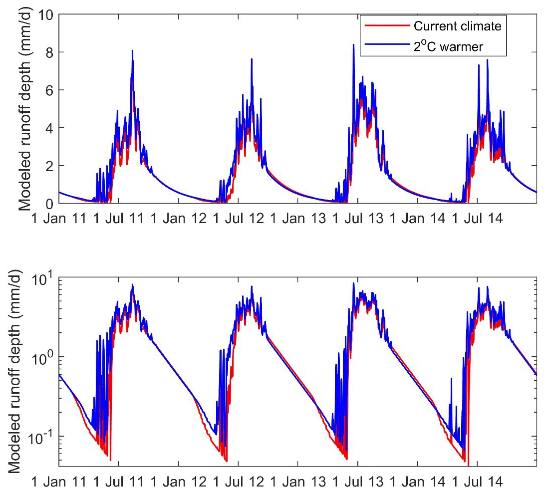
To quantify the impacts of warming on frozen soil hydrology, we arbitrarily set the air temperature to increase by 2 ∘C. The FLEX-Topo-FS simulation illustrated that the complete thaw date became 16–19 d earlier, and the lower limit of permafrost increased by 294 m, from 3716 to 4010 m. For runoff simulation, the DBR phenomenon became less obvious (Fig. 12). This is because 2 ∘C warming results in permafrost degradation, which means most permafrost is degraded to seasonal frozen soil, since the DBR was caused by the different groundwater discharge behaviors in permafrost and seasonal frozen soil areas. Especially, the first recession period was contributed by the groundwater discharge from both permafrost and seasonal frozen soil areas, and the second recession period was only from the seasonal frozen soil area. The permafrost degradation turns most permafrost into seasonal frozen soil and makes groundwater discharge nearly only from the seasonal frozen soil region and leads to more continuous baseflow recession. Eventually, warming leads to the increase in both the baseflow and runoff in early thawing seasons. The warming effect on baseflow was already widely observed in the Arctic and mountainous permafrost rivers (Ye et al., 2009; Brutsaert and Hiyama, 2012; Niu et al., 2010; Song et al., 2020; Wang et al., 2021). Hence, these wide observations could be another verification for the FLEX-Topo-FS model realism. For implications in water resource management, the results indicate that frozen soil degradation caused by climate change may largely alter the streamflow regime, especially for the thirsty spring and early summer, in the vast cold QTP. It is also worthwhile to be note that this is a primary prediction. We used 2 ∘C warmer more like a sensitivity analysis to illustrate how warming will impact on baseflow and to further verify the capability and robustness of the model itself. In future studies, we need more detailed modeling studies to use the state-of-the-art climate prediction and downscaling methodologies to assess the frozen soil changes and hydrology variations.
6.4 Implications for other cold regions
We believe that the FLEX-Topo-FS model has great potential to be applied in other cold regions. There are mainly three reasons.
First, our study site, the Hulu catchment, although small (23.1 km2), has a large elevation gradient (from 2960 to 4820 m), diverse landscapes (hillslope vegetation, riparian area, alpine desert, and glaciers), snowfall and snowmelt, and both permafrost and seasonal frozen soil. Our newly developed model explicitly considered all these spatial and temporal heterogeneities and eventually achieved excellent performance. With such a comprehensive modeling toolkit, the model has the potential to be upscaled or transferred to other cold regions.
Second, we obtained the perceptual model from not only the observations and our expert knowledge at the Hulu catchment itself, but we also widely considered the impact of frozen soil on hydrological processes in other catchments, including the Zhamashike and Qilian (two nested subcatchments of the upper Heihe), the headwater of Yellow River, and the Cape Bounty Arctic Watershed Observatory in Canada. Thus, we developed the model for the Hulu catchment in the context of larger-scale observations.
Third, the realism of the conceptual model was confirmed not only by streamflow measurement but also by multi-source and multi-scale observations, particularly the freezing and thawing front in the soil, the lower limit of permafrost, and the trends in groundwater level variation.
Although our new model generally has great potential to be used in other cold regions, we should be cautious of arbitrarily using the model without any prior understanding of the modeling system. Since frozen soil is merely one influential factor for cold region hydrology, there are other factors that have notable impacts which are intertwined with frozen soil. This relates especially to the geology condition, which can have considerable impact on frozen soil but has large spatial heterogeneity, and where it is difficult to take measurements. For the model's empirical parameters, most of them are related to the freeze–thaw processes related to Stefan equation, which have clear physical meanings and have been confirmed by previous studies with a good spatial distribution over the entire QTP (e.g., Zou et al., 2017; Ran et al., 2022). Due to the extreme complexity of soil and geology in mountainous catchments, we still need to recalibrate their values while modeling other basins on the QTP. Hence, before upscaling to other cold regions, we recommend following a stringent modeling procedure, i.e., expert-driven data analysis → qualitative perceptual model → quantitative conceptual model → testing of model realism.
Our knowledge on frozen soil hydrology is still incomplete, which is particularly true for complex mountainous catchment on the QTP. In the past few decades, we have collected numerous heterogeneities and complexities in frozen soil regions, but most of these observations are still neither well integrated into hydrological models nor used to constrain model structure or parameterization in catchment-scale studies. More importantly, we still largely lack quantitative knowledge on which variables play more dominant roles at certain spatiotemporal scales and should be included in models with priority.
By conducting this frozen soil hydrological modeling study for the complex mountainous Hulu catchment, we reached the following conclusions: (1) we observed two new phenomena in the frozen soil catchment, i.e., the low runoff in early thawing seasons (LRET) and discontinuous baseflow recession (DBR), which are widespread but not yet reported. (2) Without considering the frozen soil, the FLEX-Topo model was not able to reproduce LRET and DBR observations. (3) Considering frozen soil impacts on soil–groundwater connectivity and groundwater recession, and the FLEX-Topo-FS model successfully reproduced the LRET and DBR events. The FLEX-Topo-FS results were also verified by observing the freeze/thaw depth variation, groundwater level, and lower limit of permafrost. We believe this study is able to give us new insights into further implications to help us understand the impact of frozen soil on hydrology and project the impacts of climate change on water resources in vast cold regions, which is one of the 23 major unsolved scientific problems in the hydrology community.
The code is available upon request to the contact author.
The field work data are available upon request to the contact author.
HG, HS, FF, and KW designed the study. CH and RC provided the valuable fieldwork data, including both measured data and expert knowledge of the study site. HG, KW, and ZF conducted the analyses. HG wrote the paper. All authors discussed the results and the first draft and contributed to the final paper.
At least one of the (co-)authors is a member of the editorial board of Hydrology and Earth System Sciences. The peer-review process was guided by an independent editor, and the authors have also no other competing interests to declare.
Publisher's note: Copernicus Publications remains neutral with regard to jurisdictional claims in published maps and institutional affiliations.
We thank two anonymous reviewers, for their constructive comments and suggestions, which helped us to improve the paper.
This research has been supported by the National Natural Science Foundation of China (grant nos. 42122002, 42071081, 42171125, and 41971041).
This paper was edited by Fuqiang Tian and reviewed by two anonymous referees.
Andresen, C. G., Lawrence, D. M., Wilson, C. J., McGuire, A. D., Koven, C., Schaefer, K., Jafarov, E., Peng, S., Chen, X., Gouttevin, I., Burke, E., Chadburn, S., Ji, D., Chen, G., Hayes, D., and Zhang, W.: Soil moisture and hydrology projections of the permafrost region – a model intercomparison, The Cryosphere, 14, 445–459, https://doi.org/10.5194/tc-14-445-2020, 2020.
Beven, K. and Binley, A.: The future of distributed models: Model calibration and uncertainty prediction, Hydrol. Process., 6, 279–298, https://doi.org/10.1002/hyp.3360060305, 1992.
Blume, T., Zehe, E., and Bronstert, A.: Rainfall-runoff response, event-based runoff coefficients and hydrograph separation, Hydrol. Sci. J., 52, 843–862, https://doi.org/10.1623/hysj.52.5.843, 2007.
Blöschl, G., Bierkens, M. F. P., Chambel, A., Cudennec, C., Destouni, G., Fiori, A., Kirchner, J. W., McDonnell, J. J., Savenije, H. H. G., Sivapalan, M., Stumpp, C., Toth, E., Volpi, E., Carr, G., Lupton, C., Salinas, J., Széles, B., Viglione, A., Aksoy, H., Allen, S. T., Amin, A., Andréassian, V., Arheimer, B., Aryal, S. K., Baker, V., Bardsley, E., Barendrecht, M. H., Bartosova, A., Batelaan, O., Berghuijs, W. R., Beven, K., Blume, T., Bogaard, T., de Amorim, P. B., Böttcher, M. E., Boulet, G., Breinl, K., Brilly, M., Brocca, L., Buytaert, W., Castellarin, A., Castelletti, A., Chen, X., Chen, Y., Chen, Y., Chifflard, P., Claps, P., Clark, M. P., Collins, A. L., Croke, B., Dathe, A., David, P. C., de Barros, F. P. J., de Rooij, G., Baldassarre, G. D., Driscoll, J. M., Duethmann, D., Dwivedi, R., Eris, E., Farmer, W. H., Feiccabrino, J., Ferguson, G., Ferrari, E., Ferraris, S., Fersch, B., Finger, D., Foglia, L., Fowler, K., Gartsman, B., Gascoin, S., Gaume, E., Gelfan, A., Geris, J., Gharari, S., Gleeson, T., Glendell, M., Bevacqua, A. G., González-Dugo, M. P., Grimaldi, S., Gupta, A. B., Guse, B., Han, D., Hannah, D., Harpold, A., Haun, S., Heal, K., Helfricht, K., Herrnegger, M., Hipsey, M., Hlaváciková, H., Hohmann, C., Holko, L., Hopkinson, C., Hrachowitz, M., Illangasekare, T. H., Inam, A., Innocente, C., Istanbulluoglu, E., Jarihani, B., Kalantari, Z., Kalvans, A., Khanal, S., Khatami, S., Kiesel, J., Kirkby, M., Knoben, W., Kochanek, K., Kohnová, S., Kolechkina, A., Krause, S., Kreamer, D., Kreibich, H., Kunstmann, H., Lange, H., Liberato, M. L. R., Lindquist, E., Link, T., Liu, J., Loucks, D. P., Luce, C., Mahé, G., Makarieva, O., Malard, J., Mashtayeva, S., Maskey, S., Mas-Pla, J., Mavrova-Guirguinova, M., Mazzoleni, M., Mernild, S., Misstear, B. D., Montanari, A., Müller-Thomy, H., Nabizadeh, A., Nardi, F., Neale, C., Nesterova, N., Nurtaev, B., Odongo, V. O., Panda, S., Pande, S., Pang, Z., Papacharalampous, G., Perrin, C., Pfister, L., Pimentel, R., Polo, M. J., Post, D., Sierra, C. P., Ramos, M.-H., Renner, M., Reynolds, J. E., Ridolfi, E., Rigon, R., Riva, M., Robertson, D. E., Rosso, R., Roy, T., Sá, J. H. M., Salvadori, G., Sandells, M., Schaefli, B., Schumann, A., Scolobig, A., Seibert, J., Servat, E., Shafiei, M., Sharma, A., Sidibe, M., Sidle, R. C., Skaugen, T., Smith, H., Spiessl, S. M., Stein, L., Steinsland, I., Strasser, U., Su, B., Szolgay, J., Tarboton, D., Tauro, F., Thirel, G., Tian, F., Tong, R., Tussupova, K., Tyralis, H., Uijlenhoet, R., van Beek, R., van der Ent, R. J., van der Ploeg, M., Loon, A. F. V., van Meerveld, I., van Nooijen, R., van Oel, P. R., Vidal, J.-P., von Freyberg, J., Vorogushyn, S., Wachniew, P., Wade, A. J., Ward, P., Westerberg, I. K., White, C., Wood, E. F., Woods, R., Xu, Z., Yilmaz, K. K., and Zhang, Y.: Twenty-three unsolved problems in hydrology (UPH) – a community perspective, Hydrol. Sci. J., 64, 1141–1158, https://doi.org/10.1080/02626667.2019.1620507, 2019.
Bring, A., Fedorova, I., Dibike, Y., Hinzman, L., Mård, J., Mernild, S. H., Prowse, T., Semenova, O., Stuefer, S. L., and Woo, M. K.: Arctic terrestrial hydrology: A synthesis of processes, regional effects, and research challenges, J. Geophys. Res.-Biogeo., 121, 621–649, https://doi.org/10.1002/2015JG003131, 2016.
Brutsaert, W. and Hiyama, T.: The determination of permafrost thawing trends from long-term streamflow measurements with an application in eastern Siberia, J. Geophys. Res.-Atmos., 117, 1–10, https://doi.org/10.1029/2012JD018344, 2012.
Brutsaert, W. and Sugita, M.: Is Mongolia's groundwater increasing or decreasing? The case of the Kherlen River basin, Hydrol. Sci. J., 53, 1221–1229, https://doi.org/10.1623/hysj.53.6.1221, 2008.
Bui, M. T., Lu, J., and Nie, L.: A review of hydrological models applied in the permafrost-dominated Arctic region, Geosciences, 10, 1–27, https://doi.org/10.3390/geosciences10100401, 2020.
Cao, B., Zhang, T., Wu, Q., Sheng, Y., Zhao, L., and Zou, D.: Permafrost zonation index map and statistics over the Qinghai–Tibet Plateau based on field evidence, Permafrost Periglac., 30, 178–194, https://doi.org/10.1002/ppp.2006, 2019.
Chadburn, S., Burke, E., Essery, R., Boike, J., Langer, M., Heikenfeld, M., Cox, P., and Friedlingstein, P.: An improved representation of physical permafrost dynamics in the JULES land-surface model, Geosci. Model Dev., 8, 1493–1508, https://doi.org/10.5194/gmd-8-1493-2015, 2015.
Chang, J., Wang, G. X., Li, C. J., and Mao, T. X.: Seasonal dynamics of suprapermafrost groundwater and its response to the freeing-thawing processes of soil in the permafrost region of Qinghai-Tibet Plateau, Sci. China Earth Sci., 58, 727–738, https://doi.org/10.1007/s11430-014-5009-y, 2015.
Chen, R., Song, Y., Kang, E., Han, C., Liu, J., Yang, Y., Qing, W., and Liu, Z.: A cryosphere-hydrology observation system in a small alpine watershed in the Qilian mountains of China and its meteorological gradient, Arct., Antarct. Alp. Res., 46, 505–523, https://doi.org/10.1657/1938-4246-46.2.505, 2014.
Chen, R., Wang, G., Yang, Y., Liu, J., Han, C., Song, Y., Liu, Z., and Kang, E.: Effects of Cryospheric Change on Alpine Hydrology: Combining a Model With Observations in the Upper Reaches of the Hei River, China, J. Geophys. Res.-Atmos., 123, 3414–3442, https://doi.org/10.1002/2017JD027876, 2018.
Chiasson-Poirier, G., Franssen, J., Lafrenière, M. J., Fortier, D., and Lamoureux, S. F.: Seasona evolution of active layer thaw depth and hillslope-stream connectivity in a permafrost watershed, Water Resour. Res., 56, 1–18, https://doi.org/10.1029/2019WR025828, 2020.
Cuo, L., Zhang, Y., Bohn, T. J., Zhao, L., Li, J., Liu, Q., and Zhou, B.: Journal of geophysical research, Nature, 175, 238, https://doi.org/10.1038/175238c0, 2015.
Ding, Y., Zhang, S., Chen, R., Han, T., Han, H., Wu, J., Li, X., Zhao, Q., Shangguan, D., Yang, Y., Liu, J., Wang, S., Qin, J., and Chang, Y.: Hydrological Basis and Discipline System of Cryohydrology: From a Perspective of Cryospheric Science, Front. Earth Sci., 8, 574707, https://doi.org/10.3389/feart.2020.574707, 2020.
Dobinski, W.: Permafrost, Earth-Sci. Rev., 108, 158–169, 2011.
Evans, S. G., Ge, S., Voss, C. I., and Molotch, N. P.: The Role of Frozen Soil in Groundwater Discharge Predictions for Warming Alpine Watersheds, Water Resour. Res., 54, 1599–1615, https://doi.org/10.1002/2017WR022098, 2018.
Fabre, C., Sauvage, S., Tananaev, N., Srinivasan, R., Teisserenc, R., and Pérez, J. M. S.: Using modeling tools to better understand permafrost hydrology, Water (Switzerland), 9, 418, https://doi.org/10.3390/w9060418, 2017.
Farquharson, L. M., Romanovsky, V. E., Cable, W. L., Walker, D. A., Kokelj, S. V., and Nicolsky, D.: Climate Change Drives Widespread and Rapid Thermokarst Development in Very Cold Permafrost in the Canadian High Arctic, Geophys. Res. Lett., 46, 6681–6689, https://doi.org/10.1029/2019GL082187, 2019.
Fenicia, F. and McDonnell, J. J.: Modeling streamflow variability at the regional scale: (1) perceptual model development through signature analysis, J. Hydrol., 605, 127287, https://doi.org/10.1016/j.jhydrol.2021.127287, 2022.
Fenicia, F., Savenije, H. H. G., Matgen, P., and Pfister, L.: Is the groundwater reservoir linear? Learning from data in hydrological modelling, Hydrol. Earth Syst. Sci., 10, 139–150, https://doi.org/10.5194/hess-10-139-2006, 2006.
Gao, H.: Landscape-based hydrological modelling: understanding the influence of climate, topography, and vegetation on catchment hydrology, PhD Dissertation, Delft University of Technology, 2015.
Gao, H., Hrachowitz, M., Sriwongsitanon, N., Fenicia, F., Gharari, S., and Savenije, H. H. G.: Accounting for the influence of vegetation and landscape improves model transferability in a tropical savannah region, Water Resour. Res., 52, 7999–8022, https://doi.org/10.1002/2016WR019574, 2016.
Gao, H., Hrachowitz, M., Fenicia, F., Gharari, S., and Savenije, H. H. G.: Testing the realism of a topography-driven model (FLEX-Topo) in the nested catchments of the Upper Heihe, China, Hydrol. Earth Syst. Sci., 18, 1895–1915, https://doi.org/10.5194/hess-18-1895-2014, 2014.
Gao, H., Ding, Y., Zhao, Q., Hrachowitz, M., and Savenije, H. H. G.: The importance of aspect for modelling the hydrological response in a glacier catchment in Central Asia, Hydrol. Process., 31, 2842–2859, https://doi.org/10.1002/hyp.11224, 2017.
Gao, H., Dong, J., Chen, X., Cai, H., Liu, Z., Jin, Z., Mao, D., Yang, Z., and Duan, Z.: Stepwise modeling and the importance of internal variables validation to test model realism in a data scarce glacier basin, J. Hydrol., 591, 125457, https://doi.org/10.1016/j.jhydrol.2020.125457, 2020.
Gao, H., Wang, J., Yang, Y., Pan, X., Ding, Y., and Duan, Z.: Permafrost Hydrology of the Qinghai-Tibet Plateau: A Review of Processes and Modeling, Front. Earth Sci., 8, 576838, https://doi.org/10.3389/feart.2020.576838, 2021.
Gao, J., Xie, Z., Wang, A., Liu, S., Zeng, Y., Liu, B., Li, R., Jia, B., Qin, P., and Xie, J.: A New Frozen Soil Parameterization Including Frost and Thaw Fronts in the Community Land Model, J. Adv. Model. Earth Sy., 11, 659–679, https://doi.org/10.1029/2018MS001399, 2019.
Gharari, S., Hrachowitz, M., Fenicia, F., Gao, H., and Savenije, H. H. G.: Using expert knowledge to increase realism in environmental system models can dramatically reduce the need for calibration, Hydrol. Earth Syst. Sci., 18, 4839–4859, https://doi.org/10.5194/hess-18-4839-2014, 2014.
Gisnås, K., Westermann, S., Schuler, T. V., Melvold, K., and Etzelmüller, B.: Small-scale variation of snow in a regional permafrost model, The Cryosphere, 10, 1201–1215, https://doi.org/10.5194/tc-10-1201-2016, 2016.
Gouttevin, I., Krinner, G., Ciais, P., Polcher, J., and Legout, C.: Multi-scale validation of a new soil freezing scheme for a land-surface model with physically-based hydrology, The Cryosphere, 6, 407–430, https://doi.org/10.5194/tc-6-407-2012, 2012.
Gupta, H. V., Kling, H., Yilmaz, K. K., and Martinez, G. F.: Decomposition of the mean squared error and NSE performance criteria: Implications for improving hydrological modelling, J. Hydrol., 377, 80–91, https://doi.org/10.1016/j.jhydrol.2009.08.003, 2009.
Han, C., Chen, R., Liu, J., Yang, Y., and Liu, Z.: Hydrological characteristics in non-freezing period at the alpine desert zone of Hulugou watershed, Qilian Mountains, J. Glaciol. Geocryol., 35, 1536–1544, 2013.
Han, C., Chen, R., Liu, Z., Yang, Y., Liu, J., Song, Y., Wang, L., Liu, G., Guo, S., and Wang, X.: Cryospheric Hydrometeorology Observation in the Hulu Catchment (CHOICE), Qilian Mountains, China, Vadose Zone J., 17, 180058, https://doi.org/10.2136/vzj2018.03.0058, 2018.
He, Z., Duethmann, D., and Tian, F.: A meta-analysis based review of quantifying the contributions of runoff components to streamflow in glacierized basins. J. Hydrol., 603, 126890, https://doi.org/10.1016/j.jhydrol.2021.126890, 2021.
Immerzeel, W. W., Van Beek, L. P. H., and Bierkens, M. F. P.: Climate change will affect the asian water towers, Science, 328, 1382–1385, https://doi.org/10.1126/science.1183188, 2010.
Immerzeel, W. W., Wanders, N., Lutz, A. F., Shea, J. M., and Bierkens, M. F. P.: Reconciling high-altitude precipitation in the upper Indus basin with glacier mass balances and runoff, Hydrol. Earth Syst. Sci., 19, 4673–4687, https://doi.org/10.5194/hess-19-4673-2015, 2015.
Jarvis, P. G.: Prospects for bottom-up models, in: Scaling Physiological Processes: Leaf to Globe, edited by: Ehleringer J. R. and Field, C. B., Academic Press, 1993.
Jiang, H., Zheng, G., Yi, Y., Chen, D., Zhang, W., Yang, K., and Miller, C. E.: Progress and Challenges in Studying Regional Permafrost in the Tibetan Plateau Using Satellite Remote Sensing and Models, Front. Earth Sci., 8, 560403, https://doi.org/10.3389/feart.2020.560403, 2020.
Kurylyk, B. L., Hayashi, M., Quinton, W. L., McKenzie, J. M., and Voss, C. I.: Influence of vertical and lateral heat transfer on permafrost thaw, peatland landscape transition, and groundwater flow, Water Resour. Res., 52, 1286–1305, https://doi.org/10.1002/2015WR018057, 2016.
Lafrenière, M. J. and Lamoureux, S. F.: Effects of changing permafrost conditions on hydrological processes and fluvial fluxes, Earth-Sci. Rev., 191, 212–223, 2019.
Li, X., Wu, T., Zhu, X., Jiang, Y., Hu, G., Hao, J., Ni, R., Li, Y., Qiao, C., Yang, W., Ma, A., and Wen, X. Y.: Improving the Noah-MP model for simulating hydrothermal regime of the active layer in the permafrost regions of the Qinghai-Tibet Plateau, J. Geophys. Res.-Atmos., 125, e2020JD032588, https://doi.org/10.1029/2020JD032588, 2020.
Lindstrom, G., Bishop, K., and Lofvenius, M. O.: Soil frost and runoff at Svartberget, northern Sweden – measurements and model analysis, Hydrol. Process., 16, 3379–3392, 2002.
Liu, Y., Zhao, L., and Li, R.: Simulation of the soil water-thermal features within the active layerin Tanggula region, Tibetan plateau, by using SHAW model, J. Glaciol. Geocryol. 35, 280–290, 2013.
Ma, R., Sun, Z., Hu, Y., Chang, Q., Wang, S., Xing, W., and Ge, M.: Hydrological connectivity from glaciers to rivers in the Qinghai–Tibet Plateau: roles of suprapermafrost and subpermafrost groundwater, Hydrol. Earth Syst. Sci., 21, 4803–4823, https://doi.org/10.5194/hess-21-4803-2017, 2017.
Ma, R., Sun, Z., Chang, Q., Ge, M., and Pan, Z.: Control of the interactions between stream and groundwater by permafrost and seasonal frost in an alpine catchment, northeastern Tibet Plateau, China, J. Geophys. Res.-Atmos., 126, e2020JD033689, https://doi.org/10.1029/2020JD033689, 2021.
McNamara, J. P., Kane, D. L., and Hinzman, L. D.: An analysis of streamflow hydrology in the Kuparuk River Basin, Arctic Alaska: A nested watershed approach, J. Hydrol., 206, 39–57, https://doi.org/10.1016/S0022-1694(98)00083-3, 1998.
Nash, J. and Sutcliffe, J. V.: River Flow Forecasting through Conceptual Models Part I – A Discussion of Principles, J. Hydrol., 10, 282–290, https://doi.org/10.1016/0022-1694(70)90255-6, 1970.
Niu, G. Y. and Yang, Z. L.: Effects of frozen soil on snowmelt runoff and soil water storage at a continental scale, J. Hydrometeorol., 7, 937–952, https://doi.org/10.1175/JHM538.1, 2006.
Niu, L., Ye, B. S., Li, J., and Yu, S.: Effect of permafrost degradation on hydrological processes in typical basins with various permafrost coverage in Western China, Sci. China Earth Sci., 54, 615–624, https://doi.org/10.1007/s11430-010-4073-1, 2010.
Nitze, I., Grosse, G., Jones, B. M., Romanovsky, V. E., and Boike, J.: Remote sensing quantifies widespread abundance of permafrost region disturbances across the Arctic and Subarctic, Nat. Commun., 9, 1–11, https://doi.org/10.1038/s41467-018-07663-3, 2018.
Nyberg, L.: Soil frost effects on soil water and runoff dynamics along a boreal forest transect: 1. Field investigations, Hydrol. Process., 15, 909–926, 2001.
Oleson, K. and Lawrence, D.: NCAR / TN-503 + STR NCAR Technical Note July 2013 Technical Description of version 4.5 of the Community Land Model (CLM), (March 2014), 2013.
Osuch, M., Wawrzyniak, T. and Nawrot, A.: Diagnosis of the hydrology of a small Arctic permafrost catchment using HBV conceptual rainfall-runoff model, Hydrol. Res., 50, 459–478, https://doi.org/10.2166/nh.2019.031, 2019.
Pan, X., Li, Y., Yu, Q., Shi, X., Yang, D., and Roth, K.: Effects of stratified active layers on high-altitude permafrost warming: a case study on the Qinghai–Tibet Plateau, The Cryosphere, 10, 1591–1603, https://doi.org/10.5194/tc-10-1591-2016, 2016.
Pan, Z., Ma, R., Sun, Z., Hu, Y., Chang, Q., Ge, M., Wang, S., Bu, J., Long, X., Pan, Y., and Zhao, L.: Integrated hydrogeological and hydrogeochemical dataset of an alpine catchment in the northern Qinghai–Tibet Plateau, Earth Syst. Sci. Data, 14, 2147–2165, https://doi.org/10.5194/essd-14-2147-2022, 2022.
Ran, Y., Li, X., Cheng, G., Che, J., Aalto, J., Karjalainen, O., Hjort, J., Luoto, M., Jin, H., Obu, J., Hori, M., Yu, Q., and Chang, X.: New high-resolution estimates of the permafrost thermal state and hydrothermal conditions over the Northern Hemisphere, Earth Syst. Sci. Data, 14, 865–884, https://doi.org/10.5194/essd-14-865-2022, 2022.
Romanovsky, V. E. and Osterkamp, T. E.: Effects of unfrozen water on heat and mass transport processes in the active layer and permafrost, Permafrost Periglac., 11, 219–239, 2000.
Savenije, H. H. G.: HESS Opinions “The art of hydrology”, Hydrol. Earth Syst. Sci., 13, 157–161, https://doi.org/10.5194/hess-13-157-2009, 2009.
Savenije, H. H. G.: HESS Opinions “Topography driven conceptual modelling (FLEX-Topo)”, Hydrol. Earth Syst. Sci., 14, 2681–2692, https://doi.org/10.5194/hess-14-2681-2010, 2010.
Seibert, J. and McDonnell, J. J.: On the dialog between experimentalist and modeler in catchment hydrology: Use of soft data for multicriteria model calibration, Water Resour. Res., 38, 23-1–23-14, https://doi.org/10.1029/2001wr000978, 2002.
Shanley, J. B. and Chalmers, A.: The effect of frozen soil on snowmelt runoff at Sleepers River, Vermont, Hydrol. Process., 13, 1843–1857, https://doi.org/10.1002/(SICI)1099-1085(199909)13:12/13<1843::AID-HYP879>3.0.CO;2-G, 1999.
Sheng, Y.: Map of permafrost distribution in the Qilian Mountains. National Tibetan Plateau Data Center [data set], https://doi.org/10.11888/Geocry.tpdc.270456, 2020.
Sivapalan, M., Blöschl, G., Zhang, L., and Vertessy, R.: Downward approach to hydrological prediction, Hydrol. Process., 17, 2101–2111, https://doi.org/10.1002/hyp.1425, 2003.
Song, C., Wang, G., Mao, T., Dai, J., and Yang, D.: Linkage between permafrost distribution and river runoff changes across the Arctic and the Tibetan Plateau, Sci. China Earth Sci., 63, 292–302, 2020.
Streletskiy, D. A., Tananaev, N. I., Opel, T., Shiklomanov, N. I., Nyland, K. E., Streletskaya, I. D., Tokarev, I., and Shiklomanov, A. I.: Permafrost hydrology in changing climatic conditions: Seasonal variability of stable isotope composition in rivers in discontinuous permafrost, Environ. Res. Lett., 10, 095003, https://doi.org/10.1088/1748-9326/10/9/095003, 2015.
Sun, A., Yu, Z., Zhou, J., Acharya, K., Ju, Q., Xing, R., Huang, D., and Wen, L.: Quantified hydrological responses to permafrost degradation in the headwaters of the Yellow River (HWYR) in High Asia, Sci. Total Environ., 712, 135632, https://doi.org/10.1016/j.scitotenv.2019.135632, 2020.
Tananaev, N., Teisserenc, R., and Debolskiy, M.: Permafrost hydrology research domain: Process-based adjustment, Hydrology, 7, 6, https://doi.org/10.3390/hydrology7010006, 2020.
Walvoord, M. A. and Kurylyk, B. L.: Hydrologic Impacts of Thawing Permafrost-A Review, Vadose Zone J., 15, vzj2016.01.0010, https://doi.org/10.2136/vzj2016.01.0010, 2016.
Wang, G. X., Mao, T. X., Chang, J., Song, C. L., and Huang, K. W.: Processes of runoff generation operating during the spring and autumn seasons in a permafrost catchment on semi-arid plateaus, J. Hydrol. 550, 307–317, https://doi.org/10.1016/j.jhydrol.2017.05.020, 2017.
Wang, L., Koike, T., Yang, K., Jin, R., and Li, H.: Frozen soil parameterization in a distributed biosphere hydrological model, Hydrol. Earth Syst. Sci., 14, 557–571, https://doi.org/10.5194/hess-14-557-2010, 2010.
Wang, P., Huang, Q., Pozdniakov, S. P., Liu, S., Ma, N., Wang, T., Zhang, Y., Yu, J., Xie, J., Fu, G., Frolova, N. L., and Liu, C.: Potential role of permafrost thaw on increasing Siberian river discharge, Environ. Res. Lett., 16, 034046, https://doi.org/10.1088/1748-9326/abe326, 2021.
Wang, Q. F., Jin, H. J., Zhang, T. J., Wu, Q. B., Cao, B., Peng, X. Q., Wang, K., and Li, L. L. : Active layer seasonal freeze-thaw processes and influencing factors in the alpine permafrost regions in the upper reaches of the Heihe River in Qilian Mountains, Chin. Sci. Bull., 61, 2742–2756, https://doi.org/10.1360/N972015-01237, 2016 (in Chinese).
Wang, T., Yang, D., Yang, Y., Piao, S., Li, X., Cheng, G., and Fu, B.: Permafrost thawing puts the frozen carbon at risk over the Tibetan Plateau, Sci. Adv., 6, 2–10, https://doi.org/10.1126/sciadv.aaz3513, 2020.
Wang, Y., Yang, H., Gao, B., Wang, T., Qin, Y., and Yang, D.: State Key Laboratory of Hydroscience and Engineering, Department of Hydraulic School of Water Resources and Environment, China University of Geosciences, 2018.
Watson, V., Kooi, H., and Bense, V.: Potential controls on cold-season river flow behavior in subarctic river basins of Siberia, J. Hydrol., 489, 214–226, https://doi.org/10.1016/j.jhydrol.2013.03.011, 2013.
Woo, M.-K.: Permafrost Hydrology, Springer Berlin, Heidelberg, 564 pp., https://doi.org/10.1007/978-3-642-23462-0, 2012.
Wu, T., Li, S., Cheng, G., and Nan, Z.: Using ground-penetrating radar to detect permafrost degradation in the northern limit of permafrost on the Tibetan Plateau, Cold Reg. Sci. Technol., 41, 211–219, https://doi.org/10.1016/j.coldregions.2004.10.006, 2005.
Xiao, Y., Zhao, L., Dai, Y., Li, R., Pang, Q. and Yao, J.: Representing permafrost properties in CoLM for the Qinghai-Xizang (Tibetan) Plateau, Cold Reg. Sci. Technol., 87, 68–77, https://doi.org/10.1016/j.coldregions.2012.12.004, 2013.
Xie, C. and Gough, W. A.: Short Communication: A Simple Thaw-Freeze Algorithm for a Multi-Layered Soil using the Stefan Equation, Permafrost Periglac., 24, 252–260, 2013.
Yang, Y., Wu, Q., Jin, H., Wang, Q., Huang, Y., Luo, D., Gao, S., and Jin, X.: Delineating the hydrological processes and hydraulic connectivities under permafrost degradation on Northeastern Qinghai-Tibet Plateau, China, J. Hydrol., 569, 359–372, https://doi.org/10.1016/j.jhydrol.2018.11.068, 2019.
Ye, B., Yang, D., Zhang, Z., and Kane, D. L.: Variation of hydrological regime with permafrost coverage over Lena Basin in Siberia, J. Geophys. Res.-Atmos., 114, D07102, https://doi.org/10.1029/2008JD010537, 2009.
Zhang, R., Liu, J., Gao, H., and Mao, G.: Can multi-objective calibration of streamflow guarantee better hydrological model accuracy?, J. Hydroinformatics, 20, 687–698, https://doi.org/10.2166/hydro.2018.131, 2018.
Zhang, T., Frauenfeld, O. W., Serreze, M. C., Etringer, A., Oelke, C., McCreight, J., Barry, R. G., Gilichinsky, D., Yang, D., Ye, H., Ling, F., and Chudinova, S.: Spatial and temporal variability in active layer thickness over the Russian Arctic drainage basin, J. Geophys. Res.-Atmos., 110, 1–14, https://doi.org/10.1029/2004JD005642, 2005.
Zhao, L., Zou, D., Hu, G., Du, E., Pang, Q., Xiao, Y., Li, R., Sheng, Y., Wu, X., Sun, Z., Wang, L., Wang, C., Ma, L., Zhou, H., and Liu, S.: Changing climate and the permafrost environment on the Qinghai–Tibet (Xizang) plateau, Permafrost Periglac., 31, 396–405, https://doi.org/10.1002/ppp.2056, 2020.
Zhou, J., Kinzelbach, W., Cheng, G., Zhang, W., He, X., and Ye, B.: Monitoring and modeling the influence of snow pack and organic soil on a permafrost active layer, qinghai-tibetan plateau of china, Cold Reg. Sci. Technol., 90–91, 38–52, https://doi.org/10.1016/j.coldregions.2013.03.003, 2013.
Zou, D., Zhao, L., Wu, T., Wu, X., Pang, Q., and Wang, Z.: Modeling ground surface temperature by means of remote sensing data in high-altitude areas: test in the central Tibetan Plateau with application of moderate-resolution imaging spectroradiometer Terra/Aqua land surface temperature and ground-based infrared, J. Appl. Remote Sens., 8, 083516, https://doi.org/10.1117/1.jrs.8.083516, 2014.
- Abstract
- Introduction
- Study site and data
- An expert-driven perceptual frozen soil hydrology model based on field observations
- A semi-distributed conceptual frozen soil hydrology model
- Testing the realism of FLEX-Topo-FS model
- Discussion
- Conclusions
- Code availability
- Data availability
- Author contributions
- Competing interests
- Disclaimer
- Acknowledgements
- Financial support
- Review statement
- References