Evaluating downscaling methods of GRACE (Gravity Recovery and Climate Experiment) data: a case study over a fractured crystalline aquifer in southern India

GRACE (Gravity Recovery and Climate Experiment) and its follow-on mission have provided since 2002 monthly anomalies of total water storage (TWS), which are very relevant to assess the evolution of groundwater storage (GWS) at global and regional scales. However, the use of GRACE data for groundwater irrigation management is limited by their coarse (≃300 km) resolution. The last decade has thus seen numerous attempts to downscale GRACE data at higher – typically several tens of kilometres – resolution and to compare the downscaled GWS data with in situ measurements. Such comparison has been classically made in time, offering an estimate of the static performance of downscaling (classic validation). The point is that the performance of GWS downscaling methods may vary in time due to changes in the dominant hydrological processes through the seasons. To fill the gap, this study investigates the dynamic performance of GWS downscaling by developing a new metric for estimating the downscaling gain (new validation) against non-downscaled GWS. The new validation approach is tested over a 113 000 km² fractured granitic aquifer in southern India. GRACE TWS data are downscaled at 0.5^∘ (≃50 km) resolution with a data-driven method based on random forest. The downscaling performance is evaluated by comparing the downscaled versus in situ GWS data over a total of 38 pixels at 0.5^∘ resolution. The spatial mean of the temporal Pearson correlation coefficient (R) and the root mean square error (RMSE) are 0.79 and 7.9 cm respectively (classic validation). Confronting the downscaled results with the non-downscaling case indicates that the downscaling method allows a general improvement in terms of temporal agreement with in situ measurements (R=0.76 and RMSE = 8.2 cm for the non-downscaling case). However, the downscaling gain (new validation) is not static. The mean downscaling gain in R is about +30 % or larger from August to March, including both the wet and dry (irrigated) agricultural seasons, and falls to about +10 % from April to July during a transition period including the driest months (April–May) and the beginning of monsoon (June–July). The new validation approach hence offers for the first time a standardized and comprehensive framework to interpret spatially and temporally the quality and uncertainty of the downscaled GRACE-derived GWS products, supporting future efforts in GRACE downscaling methods in various hydrological contexts.

1 Introduction

Groundwater is an essential resource for irrigation, especially in arid and semi-arid areas. Aquifers have suffered depletion in several areas of the world these last decades, and this resource is expected to be scarcer in the future (Wada et al., 2012). Monitoring and cautious management of this resource are therefore crucial. Groundwater monitoring is traditionally achieved with networks of observation wells, but this can be challenging due to their sparse coverage, the punctual nature of the data, and the progressive abandonment of some wells or measurement difficulties and bias (Hora et al., 2019). In the meantime, new techniques for water storage monitoring have emerged with the Gravity Recovery and Climate Experiment (GRACE) satellite mission of US and German space agencies (NASA and DLR). The twin satellites of the GRACE mission were launched in 2002, and the continuity of the mission as covered by the GRACE Follow-On mission (GRACE-FO) launched in 2018. The gravimetric data retrieved from these missions have provided spatialized monthly anomalies of total water storage (TWS) for 2 decades, available worldwide. GRACE data were widely used in hydrology to study the long-term evolution of TWS or groundwater storage (GWS) by removing the contributions of other surface and sub-surface compartments from GRACE TWS at global and regional scales (Breña‐Naranjo et al., 2014; Cao and Roy, 2020; Frappart et al., 2019; Papa et al., 2015; Rodell et al., 2018; Rzepecka and Birylo, 2020; Tiwari et al., 2009; Zhang et al., 2020). Nevertheless, their application at local scale for agricultural purposes remains limited due to the very low native resolution (about 400 km) of GRACE observations (Schmidt et al., 2008; Tapley et al., 2004).

During the past decade or so, several studies have proposed methods to downscale GRACE TWS data to obtain GWS maps at a spatial resolution (typically several tens of kilometres) higher than that of GRACE observations. Those downscaling approaches can be separated into two categories: model-based downscaling and data-based downscaling (also referred in the literature as “dynamic downscaling” and “statistical downscaling” respectively). The model-based downscaling approach consists in assimilating GRACE TWS data in physically based land surface or hydrological models to obtain GWS at the temporal and spatial resolutions of the model, which are generally higher than GRACE's (Girotto et al., 2016; Houborg et al., 2012; Nie et al., 2019; Schumacher et al., 2018; Tian et al., 2017; Zaitchik et al., 2008). Yet this approach suffers from (i) the discrepancy between GRACE and model input data resolutions and (ii) the limitations inherent to models: model hypothesis and parametrization, the uncertainty of meteorological forcing, and particularly the lack of representation of anthropogenic processes such as crop irrigation (Long et al., 2013). The data-based downscaling approach consists in (i) deriving a statistical model of TWS from ancillary data available at high resolution (HR), (ii) calibrating it at low resolution (LR), (iii) applying it at HR, and (iv) removing the contribution of surface and soil moisture water stocks to isolate GWS. This data-driven approach rests on the hypothesis that the hydrological and physical processes that link those variables are identical at all resolutions (Ali et al., 2021; Jyolsna et al., 2021; Karunakalage et al., 2021; Sahour et al., 2020; Seyoum and Milewski, 2017; Vishwakarma et al., 2021; G. Zhang et al., 2021; J. Zhang et al., 2021). In the literature, data-driven methods have been used to downscale GRACE data at various scales, either at the watershed scale for a thematic approach as in Seyoum and Milewski (2017) (5000 to 20 000 km²) or grid-based, with a downscaling resolution often limited by the coarsest resolution among the predictors (Ali et al., 2021; Jyolsna et al., 2021; Ning et al., 2014; Seyoum et al., 2019; G. Zhang et al., 2021; Zhong et al., 2021; Sahour et al., 2020).

To evaluate the GRACE data downscaled from the above approaches, different strategies have been used. Table 1 lists the validation methods used in recent papers downscaling GRACE with either model-based or data-based approaches. For both method categories, the validation of downscaled GWS mostly relies on the in situ measurements of groundwater levels (GWLs), converted or not into GWS anomalies using a specific yield (Sy) representative of the study area. Note that the GWS simulated by models has been occasionally used as a reference (Houborg et al., 2012; Seyoum and Milewski, 2017). In most studies, the quality of the downscaled GWS is evaluated by comparing its time series with that of GWL or GWS derived from in situ measurements for each HR unit (spatialized – HR pixel – or localized observation well) with one or several metrics, including the coefficient of determination (R²) or Nash–Sutcliffe efficiency coefficient (NSE), the Pearson correlation coefficient (R), the root mean squared error (RMSE), or the mean absolute error (MAE) (Ali et al., 2021; Jyolsna et al., 2021; Karunakalage et al., 2021; Sahour et al., 2020; Yin et al., 2018; J. Zhang et al., 2021; G. Zhang et al., 2021; Zuo et al., 2021). In those studies, the downscaling procedure is considered efficient if those metrics fall within an acceptable range or if the downscaled product qualitatively restitutes the long-term trends of in situ data. The point is that any downscaling method can improve or degrade the accuracy of GRACE data at the targeted downscaling resolution depending on (i) the sub-pixel spatial variability of TWS/GWS and (ii) the uncertainties in input model parameters and forcing. Moreover, comparing the performances metrics with a “reference hypothesis” (here the “non-downscaled” case) allows us to quantitatively judge whether the downscaled product is better or worse in terms of accuracy at the targeted (fine) resolution and to evaluate whether the downscaling process is efficient. Therefore, quantifying the improvement against the GRACE data at their original resolution is crucial for properly evaluating downscaling methods. Among the 14 data-based methods listed in Table 1, only a few studies (Chen et al., 2019; Ning et al., 2014; J. Zhang et al., 2021; Zhong et al., 2021) quantify the improvement of the temporal agreement with in situ data of a downscaled product over the original LR data. Regarding the model-based approaches, all of them evaluate the temporal agreement of the downscaled GWS with in situ data against open-loop outputs (without the assimilation of GRACE data), but the results of the comparison against the LR GRACE TWS are not presented. Note that the primary goal of the latter methods is to improve the model simulations using GRACE data and not specifically to downscale GRACE data, even though equivalence between both objectives may be argued.

Ali et al. (2021)Chen et al. (2019)Jyolsna et al. (2021)Karunakalage et al. (2021)Ning et al. (2014)Sahour et al. (2020)Seyoum et al. (2019)Seyoum and Milewski (2017)Vishwakarma et al. (2021)Yin et al. (2018)G. Zhang et al. (2021)J. Zhang et al. (2021)Zhong et al. (2021)Zuo et al. (2021)Girotto et al. (2016)Houborg et al. (2012)Nie et al. (2019)Schumacher et al. (2018)Tian et al. (2017)Zaitchik et al. (2008)

Table 1 Validation strategies of existing – either data-based or model-based – downscaling methods of GRACE data. The downscaling method is either data-based (D) or model-based (M). The two resolutions reported are the initial resolution of GRACE data (GRACE) and the target downscaling resolution (Target). GWL: in situ groundwater level. GWS: in situ derived groundwater storage. The “Comp.” column indicates whether error statistics of the downscaled product are compared with those of another reference product: GRACE data at original low resolution (LR) or the model run in open loop (OL).

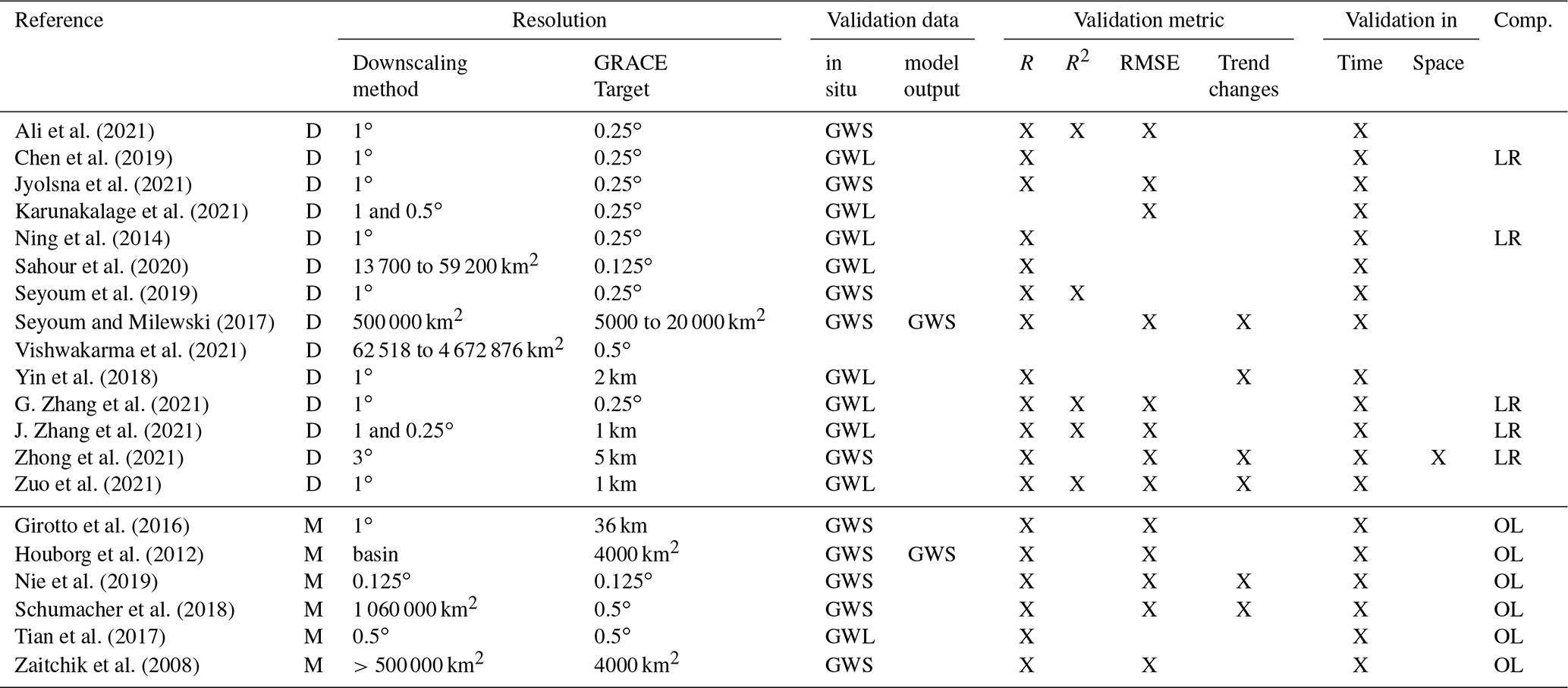
For each downscaling method, Table 1 also indicates whether the evaluation of the downscaled dataset is undertaken in time or in both time and space. Zhong et al. (2021) are the only ones proposing a validation strategy combining the time and space dimensions by measuring the improvement of RMSE and R (with monthly in situ data) from LR to downscaled GWS using 42 observation wells within the GRACE pixel and for all months of the time series. This validation approach thus combines spatial and temporal evaluations but does not isolate their individual contributions. In particular, to the knowledge of the authors, none of the previous studies has specifically evaluated the capability of downscaled products to restitute the GWS spatial variations within the GRACE pixel at the temporal observation scale (1 month in our case).

Another issue in the application and validation of current downscaling studies is the scale at which the GRACE data are used at input. The combination of the ground tracks of the GRACE twin satellites over a period of 1 month allows a native spatial resolution of 300 to 400 km for GRACE data, both for spherical harmonic (Schmidt et al., 2008; Tapley et al., 2004) and mascon solutions from the Jet Propulsion Laboratory (JPL) (Watkins et al., 2015). The GRACE TWS grids are however provided with scaling factors with resolutions of 1 and 0.5^∘ for the harmonic (Landerer and Swenson, 2012) and JPL mascon (Wiese et al., 2016) solutions respectively. Such scaling factors were originally designed to restore the lost signal of GRACE due to post-processing and to allow for averaging of the 1- or 0.5^∘-resolution oversampled TWS data over user-defined regions with a minimum extent similar to a 300–400 km-resolution GRACE pixel (Landerer and Swenson, 2012). In particular, scaling factors are not expected to efficiently downscale GRACE TWS data as neighbouring pixels are highly dependent (Landerer and Swenson, 2012). Yet many studies directly use GRACE harmonics solutions at 1^∘ resolution (Ali et al., 2021; Jyolsna et al., 2021; Karunakalage et al., 2021; Ning et al., 2014; Seyoum et al., 2019; Yin et al., 2018; J. Zhang et al., 2021; G. Zhang et al., 2021; Zuo et al., 2021) or mascon solutions at 0.5^∘ resolution (Karunakalage et al., 2021; Nie et al., 2019; Tian et al., 2017) as LR input data, which is far finer than their actual resolution. There is no study evaluating the uncertainty in downscaled GRACE data associated with the above assumption, i.e. neglecting the scale discrepancy between the actual resolution of GRACE observations and the grid size of the delivered oversampled GRACE data.

In this context, the objective of this study is to propose a consistent and complete validation framework covering the spatial and temporal aspects to quantify the supplementary information of downscaled GWS from GRACE compared with the LR original data. We test this framework on GRACE data downscaled over a granitic aquifer of 113 000 km² in Telangana in southern India. We use a data-based approach to downscale GRACE mascon solution RL06M at a 0.5^∘ resolution with two different models: a multilinear regression model and random forest. We also use this validation framework to evaluate the downscaling potential of the scaling factor at 0.5^∘ resolution provided with the mascon solution (hence evaluating the choice of using the GRACE data oversampled at 0.5^∘ resolution as a downscaled product). We compare the conclusions drawn from the classic validation techniques and the new validation framework proposed in this study.

2 Data and study area

2.1 Study area

Telangana is a highly irrigated and densely populated (about 335 inhabitants per square kilometre in 2020 according to the Unique Identification Authority of India – UIDAI) region in southern India covering 114 800 km². It is dominated by a semi-arid climate, where the monsoon precipitation occurs between July and October and ranges from 540 to 1300 mm with a mean of 879 mm (Indian Meteorological Department). The strong water demand in this area for domestic uses and the irrigation of two growing seasons a year is met with the surface water stored from monsoon rainfall and groundwater. The majority (67 000 km²) of the state is a shallow fractured granitic aquifer characterized by high fluctuations due to water pumping (Maréchal et al., 2006). It is usually composed of two layers: the first layer is saprolite, with a high effective porosity (Sy of 10 %), extending up to 10 to 15 m, and it is followed by a layer of fractured granite with a low capacity (Sy around 1 %) (Dewandel et al., 2017; Maréchal et al., 2006). This aquifer has a low capacity but strong dynamics as it fills and empties almost completely every year with monsoon rainfall and intense pumping. While continuous groundwater depletion has been observed with GRACE or observation wells in northern India (Asoka et al., 2017; Chen et al., 2014; Tiwari et al., 2009), northern China (Feng et al., 2013; Huang et al., 2015), Texas (Long et al., 2013), and many other parts of the world (Rodell et al., 2018), it is challenging to identify a long-term trend for groundwater storage in Telangana.

This study focuses on the granitic area of Telangana contoured with the 0.5^∘-resolution GRACE RL06M scaling factor grid. The study area is estimated at 113 000 km², which is similar to the actual size of a GRACE pixel. Note that the GRACE RL06M pixels were extracted by selecting the 0.5^∘ pixels falling within the granitic area of Telangana (pixels within the pink dotted line in Fig. 1).

Figure 1 Location of the study area (dotted pink line, 113 000 km²) that delineates the granitic area of Telangana (pink area, 67 000 km², identified from Phani, 2014) with the target 0.5^∘ resolution. The number of available observation wells (black triangles) monitored by the Groundwater Department of Telangana is indicated in the centre of each of the 38 0.5^∘ pixels. The grey area indicates the extent of Hyderabad, the capital city of the state. The main rivers are indicated in blue.

2.2 Data

All data used and their sources are summarized in Table 2. Figure 2 shows time series of some of the data presented below as well as their intra-annual and interannual periodicities.

Table 2 Summary of all data used.

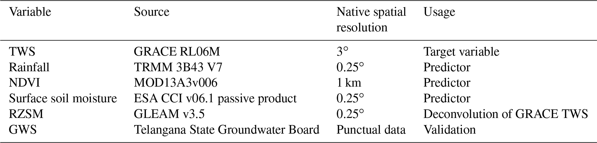
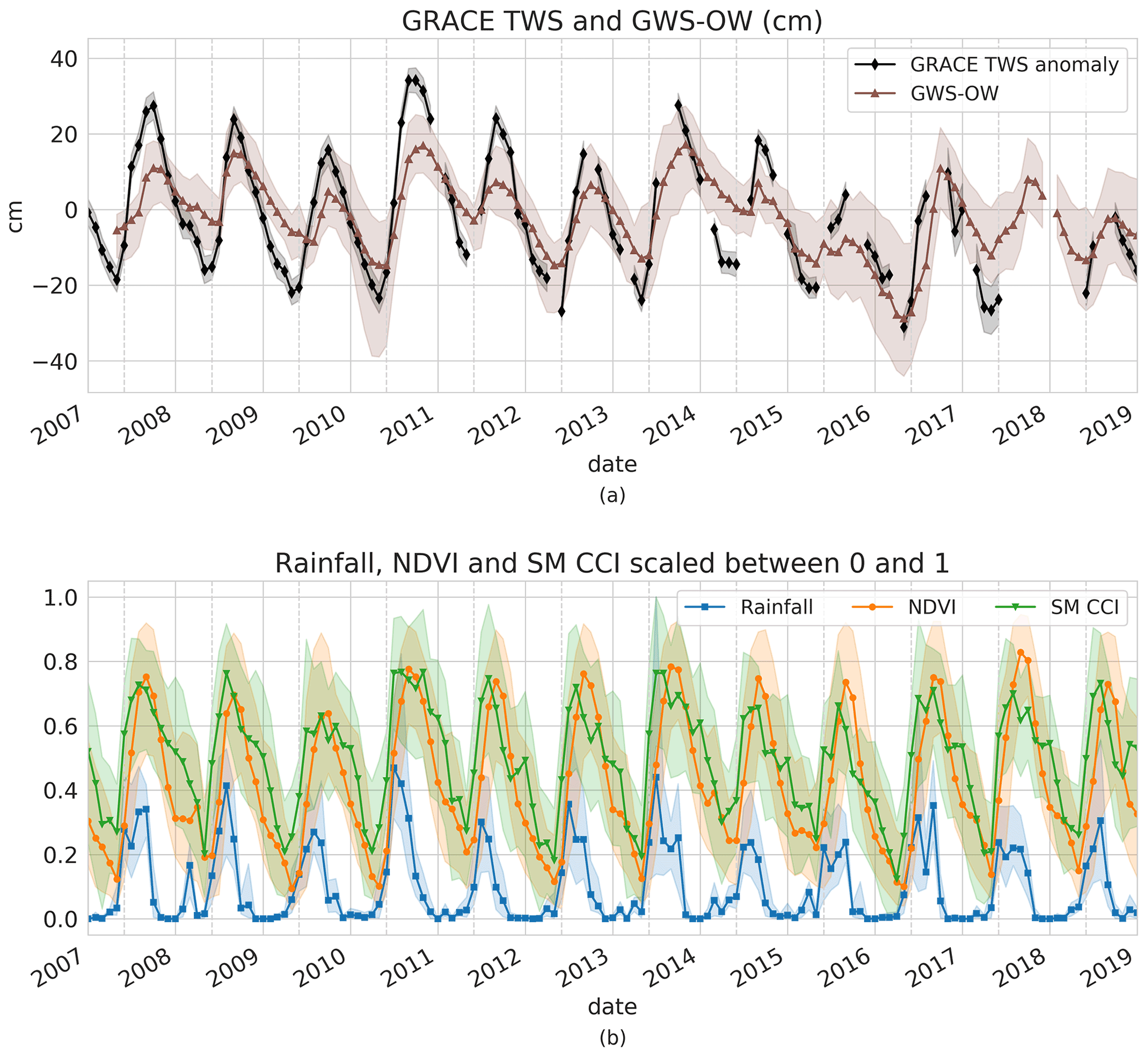
Figure 2 Time series of low-resolution (a) GRACE TWS with its uncertainty envelope (average of the mascon uncertainty resampled at 0.5^∘ provided with GRACE data) and GWS anomalies derived from in situ measurements (GWS-OW) in centimetres and (b) rainfall, NDVI and SM CCI. Those three predictors were scaled between 0 and 1 to compare their temporal cycles. The envelope for GRACE TWS is the uncertainty provided with the mascon solution, and those for GWS-OW, rainfall, NDVI and SM CCI correspond to the lowest and highest values found in high-resolution (0.5^∘) pixels at each time step. The months of June (beginning of the monsoon) are marked by dotted vertical lines.

2.2.1 GRACE TWS

We used the state-of-the-art GRACE mascon solution from JPL (RL06M) with the Coastal Resolution Improvement (CRI) filter in this study. The mascon solution uses a priori information derived from near-global geophysical models to prevent striping. Moreover, it suffers less from leakage errors than the harmonic solution (Watkins et al., 2015) (https://grace.jpl.nasa.gov/data/choosing-a-solution/, last access: 19 January 2022). Each mascon is $\mathrm{3}{}^{\circ }\times \mathrm{3}{}^{\circ }$, and the scaling factor grid used to restore the lost signal has a 0.5^∘ resolution. After multiplication of the mascon grid by the scaling factor grid, all the 0.5^∘-resolution pixels within the study area are spatially averaged over the study area to produce a LR TWS time series at 113 000 km² scale. The baseline of TWS anomalies was modified by subtracting the long-term mean of the 2007-2015 period.

2.2.2 Ancillary data

We use ancillary variables from three different datasets to predict GRACE TWS: the monthly rainfall from the TRMM mission at a 0.25^∘ resolution, the normalized difference vegetation index (NDVI) from MODIS at 1 km and the remotely sensed surface soil moisture data from the ESA CCI product (combining passive microwave-derived soil moisture products) at 0.25^∘. All these datasets provide monthly data except the CCI soil moisture (SM CCI) product, which was temporally aggregated at a monthly scale. The temporal window aggregation varies for GRACE TWS and is not always the same as those of ancillary data, but we assumed that the effects of slightly varying windows were negligible. All datasets were aggregated with bilinear resampling both at the downscaling target resolution (0.5^∘) and at regional scale (113 000 km²). The values were converted into anomalies by subtracting the long-term mean of the 2007–2015 period.

2.2.3 Deconvolution of GRACE TWS with GLEAM

GWS is a sub-compartment of TWS, and hence the downscaled GRACE TWS is not directly comparable with in situ derived GWS. In semi-arid areas, a common assumption is generally made that the essential contributions to TWS are GWS and soil moisture (SM) storage, thus neglecting canopy, snow and surface water storage (Eq. 1):

$$\begin{array}{}\text{(1)}& \mathrm{\Delta }\mathrm{TWS}=\mathrm{\Delta }\mathrm{GWS}+\mathrm{\Delta }\mathrm{SM},\end{array}$$

with Δ representing the anomalies regarding a baseline, the 2007–2015 average in our case. In Telangana, the rivers (except the major rivers Godavari and Krishna; see Fig. 1) are not perennial and only flow for a few months during and after the monsoon. Surface water stocks are composed of large dams built on major rivers, with a cumulative capacity estimated at 113 mm (Indian National Register of Large Dams) and small reservoirs in the upstream part, with a capacity estimated at 30 mm in a previous study (Pascal et al., 2021). This potential reservoir of 143 mm represents 24 % of GRACE TWS annual fluctuation in this area during the 2002–2021 time period (600 mm), yet the reservoirs are rarely simultaneously full and, most of the time, surface water storage can be neglected. Most studies use model outputs of SM to deconvolute GRACE TWS (Ali et al., 2021; Chen et al., 2019; Jyolsna et al., 2021; Karunakalage et al., 2021; Yin et al., 2018; J. Zhang et al., 2021; Zuo et al., 2021; Sahour et al., 2020; Seyoum and Milewski, 2017; Zhong et al., 2021). We used the Global Land Evaporation Amsterdam Model (GLEAM) v3.5b monthly root zone soil moisture (RZSM) dataset to simulate SM storage, which we transform into anomalies to the baseline 2007–2015. GLEAM v3.5b is a model driven by satellite data that estimates evapotranspiration and soil moisture over a 0.25^∘-resolution grid for the period 2003–2020 (Martens et al., 2017; Miralles et al., 2011). RZSM anomalies were computed by retrieving the 2007–2015 mean.

2.2.4 Validation GWS data (GWS-OW)

We use GWL data from the Groundwater Department of Telangana (India Water Resources Information System, https://indiawris.gov.in/wris, last access: 19 January 2022) for the period 2007–2019. These data provide monthly surveys of instantaneous GWL of 1006 wells distributed over the study area (see Fig. 1). Maps of GWL at 0.5^∘ were produced from the interpolation of well data with the inverse distance weighting (IDW) method (which avoids kriging bias and provides more accurate values on data points) and were converted into a GWL anomaly by retrieving the long-term mean of the 2007–2015 period. These maps were converted to GWS maps by multiplying by a Sy that was calibrated with a linear fitting between GRACE TWS deconvoluted with GLEAM RZSM and the GWL anomaly at regional scale. The Sy was estimated at 4.7 %, which is an intermediate and consistent value between the Sy of both layers (saprolite at 10 % and fractured granite at 1 %) composing the aquifer in the study region. In the following, we designate these computed GWS anomalies as GWS-OW.

3 Downscaling and validation methods

This section details the validation method developed in this study (Sect. 3.1) that consists of a validation against an LR reference in both spatial and temporal aspects. This framework is tested on state-of-the-art statistical downscaling methods that are detailed in Sect. 3.2.

3.1 Evaluation of downscaled data

3.1.1 Gain against the “null hypothesis”

As highlighted in the introduction, a lack in the majority of publications on GRACE downscaling is the comparison of the downscaled GWS with a null hypothesis. In particular, current evaluation methods check whether metrics fall within an acceptable range that is qualitatively defined but do not quantify the improvement provided by the downscaling process from a reference hypothesis. To fill the gap of current validation strategies of the downscaling methods of GRACE data, new metrics are proposed herein to quantitatively assess the accuracy of the downscaled data compared with the data at the original GRACE resolution (null hypothesis). In this case, two LR TWS references are possible: either the spatially averaged TWS value (produced as explained in Sect. 2.2.1) or the product of the mascon solution and its scaling factor grid at 0.5^∘ resolution. In both cases, the contribution of SM to TWS is removed (using GLEAM RZSM estimates used at the 0.5^∘ target resolution) to obtain GWS, comparable with in situ data. We chose to use the averaged TWS deconvoluted with the 0.5^∘ GLEAM RZSM (further called GWS-LRref) as the LR reference. The 0.5^∘-scale factor-based product (further called SF) is used as the downscaling first guess whose performance will be compared with the downscaling techniques proposed in this paper.

We chose to compute a relative gain similarly to Merlin et al. (2015). For a given metric M measuring the agreement with the validation data (e.g. R, RMSE), the gain G is computed as follows (Eq. 2):

$$\begin{array}{}\text{(2)}& G={\displaystyle \frac{|M_{\mathrm{opt}}-M_{\mathrm{LR}}|-|M_{\mathrm{opt}}-M_{\mathrm{HR}}|}{|M_{\mathrm{opt}}-M_{\mathrm{LR}}|+|M_{\mathrm{opt}}-M_{\mathrm{HR}}|}},\end{array}$$

with M_LR the value of the metric for the GWS-LRref, M_HR its value for the downscaled GWS, and M_opt the optimal value of this metric (e.g. 1 for R, 0 for RMSE). The gain of Eq. (2) can be computed in time or in space.

3.1.2 Temporal gain at high spatial resolution

For the temporal analysis, we compute this gain in the time series of GWS on all HR pixels and for three metrics: R, R², and RMSE (Eqs. 3–5). These are temporal gains, as they measure the improvement of the agreement of the time series on each HR (0.5^∘) pixel where in situ measurements are available.

$$\begin{array}{}\text{(3)}& {\displaystyle }& {\displaystyle }{G}_R={\displaystyle \frac{|\mathrm{1}-R_{\mathrm{LR}}|-|\mathrm{1}-R_{\mathrm{HR}}|}{|\mathrm{1}-R_{\mathrm{LR}}|+|\mathrm{1}-R_{\mathrm{HR}}|}}\text{(4)}& {\displaystyle }& {\displaystyle }{G}_{R^{\mathrm{2}}}={\displaystyle \frac{|\mathrm{1}-R_{\mathrm{LR}}^{\mathrm{2}}|-|\mathrm{1}-R_{\mathrm{HR}}^{\mathrm{2}}|}{|\mathrm{1}-R_{\mathrm{LR}}^{\mathrm{2}}|+|\mathrm{1}-R_{\mathrm{HR}}^{\mathrm{2}}|}}\text{(5)}& {\displaystyle }& {\displaystyle }{G}_{\mathrm{RMSE}}={\displaystyle \frac{{\mathrm{RMSE}}_{\mathrm{LR}}-{\mathrm{RMSE}}_{\mathrm{HR}}}{{\mathrm{RMSE}}_{\mathrm{LR}}+{\mathrm{RMSE}}_{\mathrm{HR}}}}\end{array}$$

3.1.3 Spatial gain at monthly scale

For the spatial analysis, we compare the monthly maps of downscaled GWS with reference maps of GWS-OW. For each time step, we compute a gain over the LR reference on four metrics: the slope S of the linear regression (Eq. 6), the mean bias B (Eq. 7), R (Eq. 3), and RMSE (Eq. 5).

$$\begin{array}{}\text{(6)}& {\displaystyle }& {\displaystyle }{G}_S={\displaystyle \frac{|\mathrm{1}-S_{\mathrm{LR}}|-|\mathrm{1}-S_{\mathrm{HR}}|}{|\mathrm{1}-S_{\mathrm{LR}}|+|\mathrm{1}-S_{\mathrm{HR}}|}}\text{(7)}& {\displaystyle }& {\displaystyle }{G}_B={\displaystyle \frac{\left|B_{\mathrm{LR}}\right|-\left|B_{\mathrm{HR}}\right|}{\left|B_{\mathrm{LR}}\right|+\left|B_{\mathrm{HR}}\right|}}\end{array}$$

We expect S and R to be closer to 1 and B and RMSE closer to 0 for the downscaled product than for the LR reference. The slope is a common indicator to evaluate downscaled products, in particular for soil moisture downscaling (Merlin et al., 2015; Sabaghy et al., 2020). Indeed, the variability of GWS is expected to be higher at HR and closer to that of in situ measurements than at LR. Computing metrics for each time step rather than on the whole time series (all time steps and all HR pixels mixed) allows us for the first time to eliminate the contributions of intra-annual and interannual variations and to specifically isolate the contribution of GWS spatial variability in the GRACE sampling period.

Figure 3 Flowchart of the downscaling method.

3.2 Statistical downscaling method

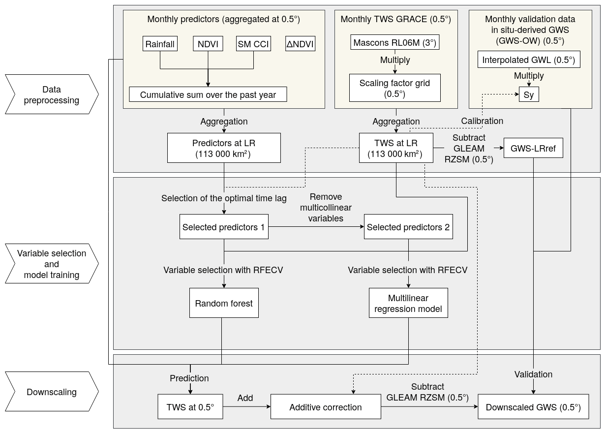
We use a data-based downscaling method that consists in training a model at LR between TWS and ancillary variables resampled at LR (113 000 km²). This model and ancillary variables at HR (0.5^∘) are then used to predict TWS at 0.5^∘. An additive correction is applied at LR to force the average of HR TWS predicted by the model to be equal to the TWS observed at LR (GRACE observation). The corrected TWS at 0.5^∘ is finally deconvoluted into GWS with the GLEAM RZSM. We compare the two models often used in the literature: the multilinear regression model and the random forest model. The downscaling process is summarized in the flowchart of Fig. 3.

3.2.1 Variable selection

For this data-driven approach, we selected remote sensing predictors that have a hydrological meaning. Also, we avoided model outputs, as irrigation is often not well represented in models. The predictors considered herein are precipitation (TRMM), surface SM (CCI), NDVI (MODIS) as an indicator of crop fraction, and the monthly variation of NDVI (ΔNDVI). We also used as predictors the cumulative sum over the past year for all variables (except ΔNDVI) by considering that it provides information about the state of the aquifer before the start of the irrigation season. Note that some predictors lag behind GRACE TWS due to the time that hydrological processes take. We determined the optimal time lag between TWS and each variable from 0 to 3 months by maximizing their temporal correlation coefficients (Sahour et al., 2020; Seyoum and Milewski, 2017). For both multilinear regression and random forest approaches, parsimonious models are obtained by selecting the optimal number of the most meaningful variables that allow prediction of the TWS. We used the RFECV (recursive feature elimination with cross-validation) algorithm, which is a greedy feature elimination algorithm similar to sequential backward selection.

3.2.2 Multilinear regression model

The multilinear (ML) regression model fits a linear relationship between the target variable Y (here TWS) and p predictors X₁, X₂, … X_p (Eq. 8):

$$\begin{array}{}\text{(8)}& Y={\mathit{\beta }}_{\mathrm{0}}+{\mathit{\beta }}_{\mathrm{1}}{X}_{\mathrm{1}}+\mathrm{\dots }+{\mathit{\beta }}_p{X}_p+E.\end{array}$$

The β₀, β₁, …, β_p are determined by minimizing the mean squared error between the data and the model predictions. This model has the advantage of being easily interpretable but is limited by the assumptions that relationships between variables are linear. Before training the ML model, the issue of multicollinearity (the existence of linear relationships between variables) was addressed. The elimination of redundant variables increases the precision of the coefficients of the regression and helps to properly identify the contribution of the remaining variables to the target variable (here TWS), and especially the signs of the coefficients. We used the variance inflation factor (VIF) (Alin, 2010) as in Sahour et al. (2020) to detect multicollinearity, and predictors with VIF > 10 were removed.

3.2.3 Random forest regressor

The random forest (RF) algorithm (Breiman, 2001) is a supervised ensemble learning algorithm composed of independent decision trees. Each decision tree learns with a subset of the predictors (here the square root of the maximum number of predictors) using a bootstrap sampling. This method softens the relationship constraints between variables but loses in interpretability. There is no need to remove some variables before training the model as the RF algorithm deals well with collinearity.

3.2.4 Additive correction

After predicting HR TWS with the ML or RF model, we corrected the TWS values so that the spatial average of HR TWS at each time step would be equal to LR TWS. We add an offset value to correct the HR TWS at each month of the time series that corresponds to the difference between LR GRACE TWS and the spatial average of HR TWS predictions at the same date (Eq. 9):

$$\begin{array}{}\text{(9)}& {\mathrm{TWS}}_{\mathrm{HR},t,i}^{\mathrm{corr}}={\mathrm{TWS}}_{\mathrm{HR},t,i}+{\mathrm{TWS}}_{\mathrm{LR},t}-{\displaystyle \frac{\sum _i{\mathrm{TWS}}_{\mathrm{HR},t,i}}{n_{\mathrm{pix}}}},\end{array}$$

with TWS${}_{\mathrm{HR},t,i}$ the HR TWS predicted by the model for month t and pixel i, TWS${}_{\mathrm{HR},t,i}^{\mathrm{corr}}$ the bias-corrected TWS, TWS_LR,t the LR TWS at date t, and $\frac{\sum _i{\mathrm{TWS}}_{\mathrm{HR},t,i}}{n_{\mathrm{pix}}}$ the spatial average of HR TWS at date t.

4 Results

This section aims at evaluating the efficiency of the two data-based downscaling methods, i.e. ML and RF models against GWS-OW. In each case, we compare these results with the first-guess downscaling product, i.e. the product of the mascon solution and its scaling factors at 0.5^∘ resolution (SF). After commenting on the results of the model calibration at LR in Sect. 4.1, we analyse the conclusions drawn from the classic evaluation methods found in the literature (Sect. 4.2) and then from the new validation method proposed in this study (Sect. 4.3). The synthesis of the different conclusions is presented in Sect. 4.4.

4.1 Variable selection and model calibration at LR

The correlation coefficients of the ancillary variables with GRACE TWS at LR are reported in Table 3. The bold correlations indicate which time lag was chosen for each variable: no lag for NDVI, 1-month lag for CCI soil moisture, 2-month lag for ΔNDVI and rainfall. The selected variables for each model are indicated in Table 4. Four variables were selected for the ML model: ΔNDVI, NDVI, SM CCI, and SM CCI accumulated over a year. The RF model selected two additional variables: monthly rainfall and rainfall accumulated over a year.

Table 3 Correlation coefficients of ancillary variables with GRACE TWS. The optimal time lag is indicated by bold correlations. The underlined correlations are not statistically significant.

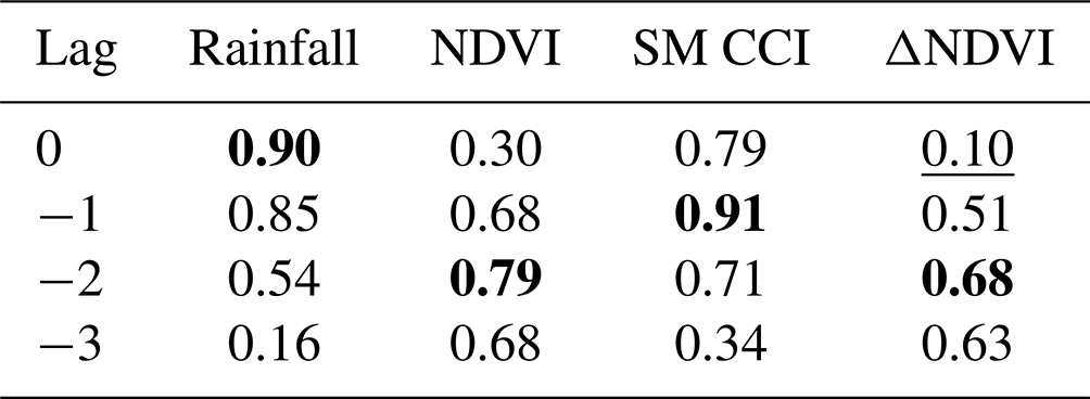
Table 4 Variable selection and model performance at LR. The number in parentheses is the number of lag months. Variables with the suffix “cum.” are cumulated over the last year. The underlined variables were eliminated with the VIF selection method. The model performance is evaluated against GRACE TWS with the R² and the RMSE on train and test sets. The R² with in situ derived TWS (sum of GWS-OW and GLEAM RZSM at LR) is also shown.

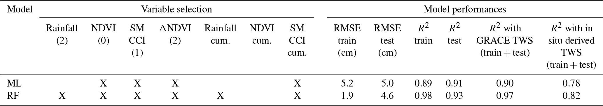
ML and RF models are trained on a random sample of 80 % of the whole time series (174 points in total). The selected variables and the model performances are reported in Table 4. The RF model has a better R² than the ML model (0.97 against 0.90), yet the RMSE and R² on the test set are far larger (lower) than on the train set (4.6 cm against 1.9 cm and 0.93 against 0.98). This reveals that the RF model suffers from overfitting due the quality of the data and the small amount of data (139 points) used to train the model, resulting in poor generalization. The RMSE on the train set is respectively 5.0 and 4.6 cm for the ML model, which represents 7 % and 6 % of the GRACE TWS total amplitude over the region during the study period (71 cm). Both models seem to be able to predict GRACE TWS with good performance. However, the performance is lower when compared with in situ data. As an example, the R² between in situ derived TWS (sum of GWS-OW and RZSM GLEAM) aggregated at LR and GRACE TWS is 0.80. This shows that only limited agreement can be expected between satellite data (or modelled from satellite data) and in situ data, because of (i) the inherent uncertainties of the data, (ii) the interpolation of in situ data, and more generally (iii) the diversity of data sources. All those uncertainty sources also apply to the TWS predicted by models at both low and high resolutions. The R² with in situ derived TWS falls from 0.90 and 0.97 to 0.78 and 0.82 for the ML and RF predictions respectively. This can be due to the existing uncertainty mentioned earlier but also to the possible lack of representativeness of in situ measurements at the GRACE spatial resolution.

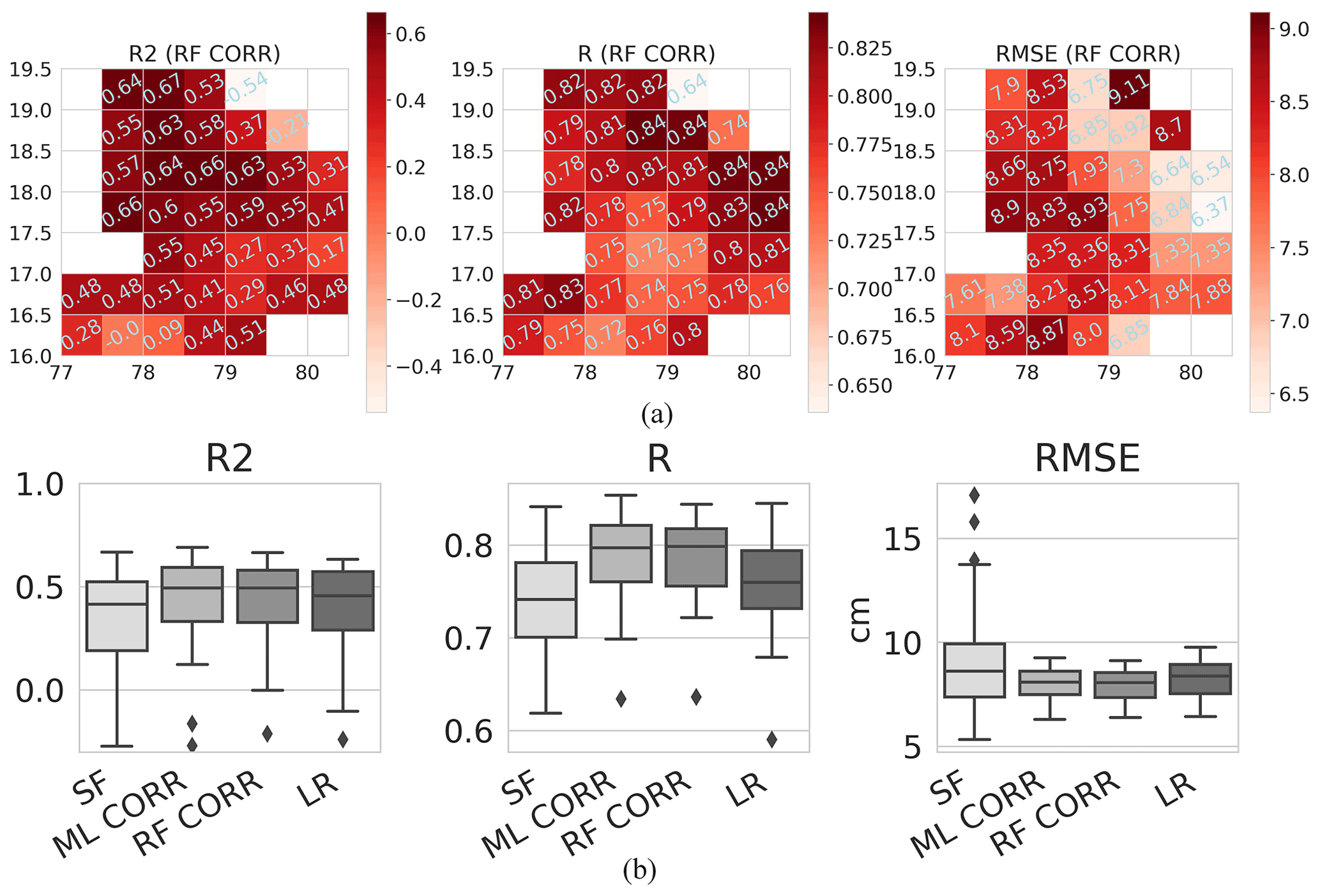
Figure 4 (a) Spatial distribution of R², R, and RMSE for the downscaling with the random forest model with bias correction (RF CORR). The numerical value of the metric is indicated in the grid. The abscissa is the east longitude and the ordinate the north latitude. (b) Boxplot (median and quartiles) of R², R, and RMSE between GWS-OW and the scaling factor product (SF), linear (ML), and random forest (RF) model-downscaled products with bias correction (CORR) and the low-resolution reference GWS-LRref (LR). The RMSE is an equivalent water height in centimetres.

4.2 Classic evaluation

The temporal agreement between GWS-OW and downscaled products was evaluated on every HR pixel with R², R, and RMSE for the SF downscaling and both the ML and RF models with correction by the LR offset value (CORR). Figure 4a shows the spatial distribution of these three metrics for the RF CORR-downscaled GWS for visualization and Fig. 4b the distribution of the three metrics on all pixels for all the downscaling methods. The temporal agreement of the SF product with GWS-OW seems to be the worst given the wide distribution of R² with an average of 0.21 and some outliers in negative values and an average RMSE of 9.1 cm. The SF product appears to perform less well than the LR reference GWS-LRref (average R², R, and RMSE of 0.38, 0.76, and 8.2 cm). The R and R² are better on average for ML CORR (0.79 and 0.42) and RF CORR (0.79 and 0.43), and the reduced variability of R and RMSE for ML CORR and RF CORR suggests that the bias correction produces results with a more uniform quality. The RMSE is still relatively large, ranging from 6.3 to 9.3 cm (6.4 to 9.3 cm) for the ML (RF) model. As a reference, the amplitude of GWS-OW in this area during the 2007–2019 time period ranges from 33 to 70 cm on all 38 HR pixels.

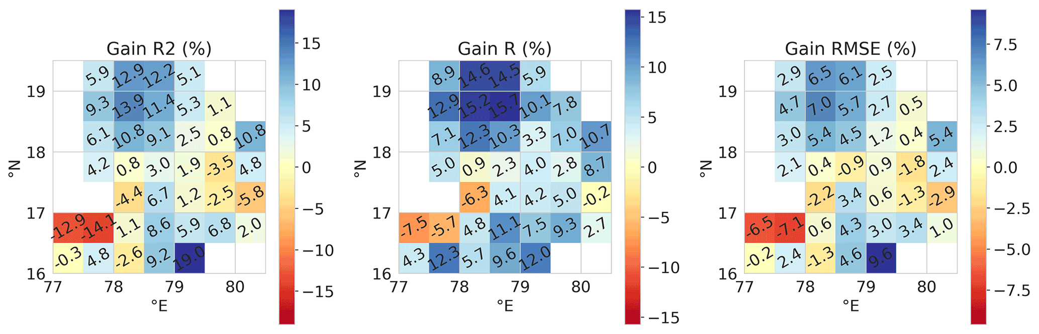
Figure 5 Spatial distribution of the gains of R², R, and RMSE for the downscaling with RF CORR. The numerical value of the metric is indicated on the grid. The abscissa is the east longitude and the ordinate the north latitude.

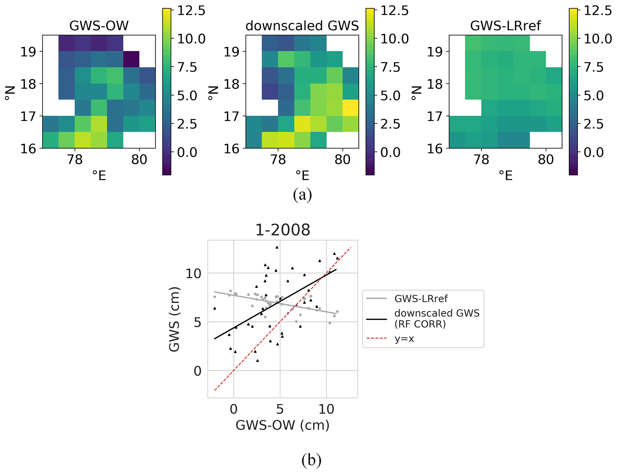
Figure 6 Illustration of the spatial gain for the month of January 2008. (a) Maps of HR in situ derived GWS (GWS-OW), RF CORR-downscaled GWS, and LR reference GWS (GWS-LRref). The abscissa is the east longitude and the ordinate the north latitude. (b) Scatterplot of the GWS-LRref (grey points) and RF-downscaled GWS (black points) against GWS-OW. The identity function is indicated by a dashed red line. The slope of the two linear regression fits on grey and black points are used to compute the gain in the slope. The differences in dispersion, uncertainty, and bias of the two point clouds are evaluated with gains in R, RMSE, and mean bias.

4.3 Evaluation with temporal and spatial gains

The temporal gains are computed as explained in Sect. 3.1 and are shown for the particular case of RF CORR in Fig. 5 for visualization. The spatial gains are computed at each time step between the two point clouds of GWS-OW and GWS-LRref or downscaled GWS, as illustrated in Fig. 6. The boxplots of temporal gains in all HR pixels and the boxplot of spatial gains in the whole time series are shown in Fig. 7. ML CORR and RF CORR show the best results: average gains in R², R, and RMSE are respectively 3.2 %, 6.5 %, and 1.55 % for ML CORR and 4.0 %, 6.7 %, and 1.9 % for RF CORR. In particular, the temporal gains for the RF CORR product seem to be positive in the north and south of the study area (cf. Fig. 5), which coincides with the two main river basins of the state but also concerns pixels with mixed geology and where the least number of observation wells are available (see Fig. 1). The pixel at 17^∘ N, 78^∘ E contains the major part of the capital city of the state, Hyderabad, a heavily urbanized area where natural hydrological processes as well as observation well measurements are highly perturbed by domestic water use, explaining the negative gains in R², R, and RMSE (−4.4 %, −6.3 %, and −2.2 % respectively).

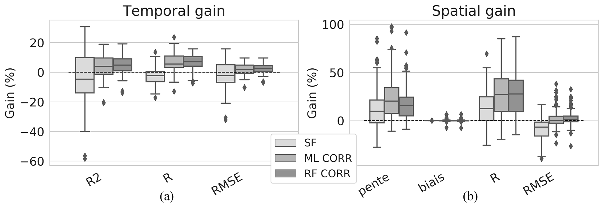
Figure 7 Boxplots (median and quartiles) of (a) temporal and (b) spatial gains for the SF, ML and RF model downscaling approaches. The CORR designation indicates that the downscaled TWS is corrected for the LR bias from GRACE data.

Figure 8 Monthly medians of spatial gains (black curves) on slope, R, and RMSE for downscaled GWS with the RF CORR model (left axis) with, on the right axis, (a) average ± standard deviation (SD) of low-resolution rainfall, NDVI, SM from the CCI dataset, and in situ derived GWS and TWS scaled between 0 and 1 and (b) interannual average ± SD of the monthly spatial variability divided by the grid maximum of rainfall, NDVI, SM from the CCI dataset, and in situ derived GWS, scaled between 0 and 1. (c) Time series of the monthly spatial variability of in situ derived GWS (red curve) with monthly cumulative rainfall (grey). The abnormally dry monsoons of 2009 and 2015 and the high GWS spatial variability during the following dry season are highlighted in black.

In the spatial domain (see Fig. 7b), the quality of the SF-downscaled GWS is questionable. The quasi-null gain in bias was expected, as the only difference between LR and SF TWS is a multiplicative factor generally close to 1. The SF-downscaled GWS shows positive gains for slope and R on most of the time series (12.9 % and 13.9 % respectively on average) but at the cost of higher uncertainty (−8.5 % gain in RMSE). Monthly scatterplots (results not shown) indicate that the slope getting closer to 1 is most of the time a consequence of an increased dispersion due to what appears to be additional noise at each time step brought by the scaling factor grid. The improvement of spatial representativity of GWS with data-based downscaling methods (ML CORR and RF CORR) is shown by overall positive gains in slopes and R (22.9 % and 28.8 % for ML CORR, 18.2 % and 27.2 % for RF CORR) while maintaining a general positive gain in RMSE as well (2.0 % and 2.2 % for ML CORR and RF CORR respectively). The bias correction at LR adjusts the HR TWS predicted by the model to the GRACE TWS amplitude, explaining the null gain in bias for both models.

Complementary to the spatial analysis of temporal metrics (e.g. in Fig. 5), the spatial gains can be analysed in time. Figure 8 shows the monthly medians of the gains in slope, R, and RMSE for RF CORR downscaled GWS. It appears that gains in slope and R are lowest during the month of July (beginning of the monsoon). Gains in both slope and R increase until January–February (beginning of the second crop season that ends in April) and decrease again. The monthly gains of RMSE have lower amplitudes than those of slope and R but have a similar pattern. The periodicity in downscaling performances is due to the capacity or incapacity of the model trained at LR to restitute the spatial variability of some intermittent processes. In this paper, the tested downscaling methods are empirical, like the majority of existing methods (Ali et al., 2021; Jyolsna et al., 2021; Sahour et al., 2020; Seyoum and Milewski, 2017). Therefore, we are not able to represent explicitly the underlying hydrological processes that explain (in the downscaling procedure) the spatial variability of GWS at a given time. However, the performance of the downscaling methods essentially relies on their capability to represent implicitly the discharge and recharge of the aquifer at 0.5^∘ resolution. This is the reason why the temporal variability in the downscaling performance can be interpreted in terms of taking into account the dominant hydrological processes and their seasonal dynamics.

In Telangana, the year can be divided into several periods given their dominant hydrological processes. The month of August marks the start of aquifer recharge by the rainfall that occurs 2 to 3 months after the beginning of the monsoon (which lasts generally from August to October; see Fig. 8a). It is also the beginning of the growing season (which typically lasts from July to November), when the monsoon rainfall stored at the surface and in the aquifer are used for irrigation. The higher spatial gains in slope, R, and RMSE during this period show that the recharge process in space is correctly represented with the precipitation data at 0.5^∘ (having mainly a north–south gradient). The period between January and March, during the dry season, is marked by the heavy pumping and use of surface water for crop irrigation. This process is relatively well represented by the downscaling model from SM CCI and NDVI data, which provide indirect information on irrigation and crop stage respectively. During this period, the spatial variability of both predictors (illustrated by Fig. 8b, which represents the interannual average of the monthly spatial variability) is relatively large, accounting for the differences in crop fraction and type that highly depend on surface water availability. By April–May, irrigation stops and groundwater reaches its lowest level. The downscaling gains obtained at that time of year are relatively low. The model probably fails to restitute the diversity of HR GWS when the water availability and thus water exchanges are very scarce and hardly inferable from the chosen predictors. At the beginning of the monsoon in June–July, heavy rainfall occurs and fills rivers and reservoirs. However, at this early stage of the monsoon, rainfall has not reached the aquifers and GWS remains low as in April and May. Also, surface water is an important component of the water column at this time of year (potentially up to 24 % of the annual fluctuation of TWS; see Sect. 2.2.3), yet runoff is not directly modelled by any of the variables of the RF model, which could also mislead the model into attributing surface water stocks to groundwater.

The use of a spatial gain also highlights the difficulties of state-of-the-art “static” downscaling methods (calibrated with constant parameters) to restitute an interannual variability. This is illustrated by Fig. 8b, which represents the interannual average (curve) and variability (envelope) of the monthly spatial variability of GWS. The interannual variability, which is lowest from August to January and highest from April to July for GWS, is inversely proportional to the downscaling performance. This result indicates that this kind of method is unable to represent the interannual variation of the dominant hydrological processes. Such a difference in interannual variability during the end of the dry season can be explained by the succession of drier and wetter periods dictated by El Niño and La Niña phenomena (Asoka et al., 2017; Vissa et al., 2019). This involves differences in yearly cumulative rainfall that determine the types of crops according to their water needs. During the driest years in particular, differences in water availability widen the gap between 0.5^∘ regions, explaining higher spatial variabilities of GWS. This is illustrated in Fig. 8c by the abnormally high GWS spatial variability following the dry monsoons of 2009 and 2015.

4.4 Comparative analysis of both validation methods

The thresholds to decide whether temporal metrics are poor, satisfactory, or good are often arbitrarily decided and are different with the context of the study and the authors' choices. In our case, all downscaled GWS products have correlation coefficients with GWS-OW systematically larger than 0.57 on each of the 38 HR pixels, which can be considered a quite satisfactory result. With the R² criteria, ML CORR and RF CORR seem to have the best performance, with at least half of the HR pixels having R² larger than 0.5. For ML CORR and RF CORR, the RMSE does not go below 6.3 and 6.7 cm respectively, with a median RMSE of 8.1 cm for both methods, which still represent a non-negligible 18 % (16 %) error against GWS-OW (GWS-LRref) amplitude at LR.

Those above appreciations of temporal metrics do not indicate the superiority and the downscaling capacity of these downscaled GWS maps over GWS-LRref. With spatial and temporal gains, it was shown that ML CORR and RF CORR products are able to improve the temporal agreement with in situ data for most of the HR pixels. In the spatial aspect, ML CORR and RF CORR both improve the spatial representativity of GWS for most of the time series (positive gains in slope and R), with a slightly lower uncertainty (gain in RMSE mostly positive). In addition to the comparison against the LR reference, the validation in both time and space allows a better understanding of the downscaling strengths and flaws depending on local characteristics of some HR pixels (e.g. presence of rivers, agricultural practices, climatological variability, or large cities) or the time of year (e.g. wet or dry season). In the temporal domain, the RF CORR downscaled GWS seems to be better correlated with in situ data in the north and south of the study area near large rivers. This suggests that the model trained at LR has difficulties in modelling certain processes, e.g. the hydrological response to anthropic pressure that is localized and thus smoothed when averaged over a larger region. In the spatial domain, our validation method shows that the RF CORR downscaled GWS performed less during the dry season and the beginning of the wet season, supposedly because the model fails to represent the spatial variability of GWS when GWS is low or when surface water represents an important fraction of TWS. This highlights the weaknesses of a static model trained on a whole time series with no regards for the specificities of the hydrologically dominant processes at several times of the year.

5 Discussion

Here we discuss how downscaled products can be impacted by (i) the resolution at which GRACE data are used (Sect. 5.1) and (ii) the uncertainty issues when combining data from heterogeneous sources (Sect. 5.2).

5.1 Impact of the GRACE actual resolution on downscaled results

The validation framework proposed in this article was used to evaluate the downscaling potential of the scaling factor built from mascon solution RL06M. The scaling factor is built by fitting a unique factor between the TWS from the GLDAS CLM model at 0.5^∘ and aggregated at mascon scale (3^∘) to evaluate the signal loss over the entire time series. Although it is not meant to downscale the mascon solution, several recent articles in the literature have used the oversampled TWS (spherical harmonics at 1^∘ or mascon solution at 0.5^∘) as the LR input data. Our validation framework clearly showed that the product of GRACE TWS mascons and their scaling factor grid (SF method) degrades the temporal agreement with in situ data and is noisy at a monthly timescale. Such results indicate that this product should not be used at the 0.5^∘ resolution.

5.2 Other uncertainty sources in the validation exercise

Another point that should be highlighted is the difficulty in validating downscaled products with in situ data. Downscaled GWS is built from remote sensing data with various acquisition processes, while validation data are derived from water-level depth acquired by local piezometers with a heterogenous distribution in the study area (see Fig. 1). Each methodological step before a possible comparison between spatialized in situ and remote-sensing-derived GWS adds uncertainties at LR, illustrated by a low R² (0.63) and high RMSE (6.1 cm) between GWS-OW and GWS-LRref.

The in situ data have their own uncertainties. First, the GWS derived from GWL measurements is highly dependent on the value of the Sy used. Here we used a horizontally and vertically homogeneous Sy, obtained with a linear adjustment between LR GWL and GWS-LRref. Some authors avoid this issue by directly comparing GRACE-downscaled GWS with GWL measurements (Karunakalage et al., 2021; Ning et al., 2014; Tian et al., 2019, 2017; Yin et al., 2018; J. Zhang et al., 2021; G. Zhang et al., 2021; Zuo et al., 2021). Another issue is that instantaneous GWL can be impacted by short- or long-term effects such as the neighbourhood pumping intensity at the moment of piezometer measurement, which cannot be detected or rectified with the monthly temporal frequency of acquisition.

The acquisition mode for GRACE is also different from in situ data – unique instantaneous measurement – and other remote sensing predictors – the average or sum of higher temporal frequency products. GRACE has a heterogeneous revisit frequency, where each 300×300 km² pixel is informed by approximately three overpasses of the GRACE satellites during the month (Tapley et al., 2004; Zaitchik et al., 2008). This can lead for example to smoothening of the GRACE anomaly by skipping extremes. Another issue in GRACE acquisition is the exclusively vertical sampling of the gravitational field that produces striping in the solution and requires post-processing that alters the signal.

6 Conclusions

To date, validation strategies for GRACE-derived downscaled products have rested essentially on the appreciation of temporal metrics or trends between downscaled products and localized in situ measurements. Yet such a validation approach is insufficient to fully assess the usefulness of the downscaling method as it suffers from a lack of (i) appropriate validation of the spatial distribution of the downscaled GRACE-derived GWS within the GRACE pixel and (ii) comparison with the results that would be obtained without downscaling (by directly using GRACE TWS at the fine scale). This article reviews the validation methods of existing downscaling methods of GRACE data, both model-based and data-based, and proposes a more extensive validation framework. In particular, a set of gains is used to evaluate the improvement of downscaled products against a low-resolution (LR) reference, including both temporal and, for the first time, spatial aspects. Such gains aim at fully determining the quality and uncertainty of downscaled GRACE-derived GWS products in a more comprehensive way.

The new validation framework is tested to evaluate the performance of two data-based downscaling approaches with multilinear (ML) and random forest (RF) models over a 113 000 km² fractured aquifer in southern India to the target resolution of 0.5^∘. The HR TWS predicted by each model is bias-corrected at each time step from the difference between the LR GRACE TWS and the average of HR TWS. We use GRACE TWS from the RL06M mascon solution for this study, which is multiplied by its 0.5^∘ scaling factor grid and averaged over the study area to produce the LR reference series. A secondary objective of the paper is to also assess the downscaling potential of the scaling factor by considering the product of mascon and scaling factor (SF) at the 0.5^∘ resolution to be a downscaled product. The comparison of the two data-based downscaling methods (bias-corrected ML and RF) with the LR reference shows an improvement in terms of correlation with in situ measurements. In the temporal domain, the spatial average gains in Pearson correlation coefficients (R) and root mean squared error (RMSE) are +6.5 % and +1.6 % ($+\mathrm{6}.$ % and +1.9 %) for ML (RF). In the spatial domain, the gains in R and RMSE are +28.8 % and +2 % (+27.2 % and +2.2 %) for ML (RF) respectively. The new validation method also confirms that the SF product cannot be used at 0.5^∘ resolution. Although the average R in HR pixels is similar for all methods (0.74, 0.74, and 0.76 for SF, ML, and RF respectively), the SF product degrades both temporal and spatial accuracies at 0.5^∘ resolution compared with the LR (without downscaling) case, showing that it cannot be used as a valid downscaling approach. The spatial analysis of temporal gains reveals a spatial heterogeneity in downscaling performances, which are particularly poor over urbanized areas. The spatial evaluation originally proposed in this study is also able to analyse the seasonality of the downscaling performance. The RF downscaling performance is lower (gains in R below +10 %) during the end of the dry season when GWS is at its lowest and at the beginning of the monsoon when surface flow, not included in the RF model, is a major process. In particular, the spatial validation presented in this study highlights, for the first time, the flaws of static GRACE downscaling methods in contexts where the dominant hydrological processes are not the same throughout the year (such as a highly irrigated semi-arid region with a wet season and a dry season as in the case of this study). This shows how complete and comprehensive validation approaches are an essential tool to interpret spatially and temporally the quality and uncertainty of the downscaled GRACE-derived GWS products and hence to better understand and improve downscaling models and their hypotheses in the future.

While the GRACE-FO mission provides continuity of spaceborne gravity change measurements, upcoming similar missions (MARVEL, Lemoine and Mandea, 2020; Lemoine et al., 2020; MAGIC, Massotti et al., 2021) plan to significantly improve the precision and quality of gravimetric estimates by proposing new configurations for the satellite constellations. Nevertheless, the specified spatial resolution for those future data still undergo strong technical limitations. Therefore, the recourse to downscaling techniques will be, at least in the medium term, the only way to obtain TWS products at a finer scale useful for basin-scale water management.