Evaporation front and its motion

The evaporation demands upon a rock or soil surface can exceed the ability of the profile to bring a sufficient amount of liquid water. A dry surface layer arises in the porous medium that enables just water vapor flow to the surface. The interface between the dry and wet parts of the profile is known as the evaporation front.

The paper gives the exact definition of the evaporation front and studies its motion. A set of differential equations governing the front motion in space is formulated. Making use of a set of measured and chosen values, a problem is formulated that illustrates the obtained theory. The problem is solved numerically, and the results are presented and discussed.

1 Introduction

Under arid or semiarid conditions, evaporation demands usually exceed the ability of an exposed porous medium to provide liquid-phase water. The water content of subsurface zones of coarse-grained rocks or sandy soils is usually far below its residual value, and consequently only the gas-phase water can flow through. These, mostly up to a few centimeters thick, zones are referred to as vapor zones, dry surface layers or evaporation zones (e.g., Yamanaka and Yonetani, 1999; Saravanapavan and Salvucci, 2000; Shokri et al., 2009; Deol et al., 2014).

The extent and development of the dry surface layer significantly affect the material's decay: directly by changes in its wetness, by frost and particularly by salt weathering, since dissolved salts are transported by the capillary water and form crystals at places of evaporation (e.g., Rijniers et al., 2005; Mol and Viles, 2013; Kurtzman et al., 2016).

The phenomenon is preconditioned by the fact that the porous medium becomes impervious to the liquid-phase water if the water content becomes sufficiently small. A limit arises inside the porous medium behind which the transport of water is only possible in the form of vapor. Such a soil profile can be divided into two parts that can be referred to as the zone of water flow and the zone of vapor diffusion. This formulation, however, is too vague and leaves the intermediate zone, its extent and its nature unclear.

Several studies were published, giving a detailed description of the evaporation process and the development of the transition zone (e.g., Lehmann et al., 2008; Shokri et al., 2010; Sakai et al., 2011; Or et al., 2013; Assouline et al., 2013; Rothfuss et al., 2015). These papers are mostly focused on special problems, unlike the present paper, which studies the three-dimensional problem under general transport conditions.

Sakai et al. (2011) studied the problem, considering both hydraulic and thermal processes, and detected a narrow transition layer at the bottom of the dry surface layer. Another approach (Konukcu et al., 2004) connects the interface between the region of water flow and the region of vapor flow, denoted as the evaporation front, with a critical value of the water content that can be determined directly from such porous-medium characteristics as hydraulic conductivity and vapor diffusivity.

Hadley (1982) studied the problem of water vapor transport through a region of dry material from a receding evaporation front. In the paper, the heat balance equation was involved in the final system of equations, the evaporation front was considered to be a sharp interface between the saturated zone and the dry (without liquid water) zone, the front was fixed and given a priori, and the liquid water was unmovable.

Kulikovskii (2002) studied the time–space development of discontinuities in a one-dimensional porous medium. Liquid water, vapor and mixture of liquid water and vapor were assumed in the void space, and two governing equations, water and heat flow, were considered. No particular interfaces were defined, and discontinuities, in general, were studied in time–space. Il'ichev and Shargatov (2013) started their study with similar assumptions concerning the governing laws and investigated the resulting transition surfaces and conditions of loss of their stability.

Unlike these studies, the present paper aims to define the evaporation front by means of porous-medium characteristics and to formulate the law of its motion generally not involving any particular law governing the water transport. This approach makes it possible to use any set of flow and transport laws when formulating a problem of the evaporation front motion.

Several methods using dyes were developed to visualize the dry and wet regions within soil or rock profiles (e.g., Shokri et al., 2009; Bruthans et al., 2018; Kumar and Arakeri, 2018; Weiss et al., 2018). These methods proved their efficiency in laboratory conditions when utilized to visualize the dry surface layers and, in particular, the evaporation front positions. The applied water–dye solutions increase their concentration at places of evaporation and indicate these places by changing their color.

A special method was developed (Weiss et al., 2020) that minimizes the medium destruction and is usable under the field conditions. A very thin rod covered by a layer of color is inserted into a narrow hole drilled to the investigated material where there is the sought evaporation front. The present liquid-phase water colors the corresponding part of the rod showing its extent.

A number of experiments aiming at seeking and visualizing the evaporation front, see Weiss et al. (2018) and Weiss et al. (2020), show that its position can be detected as a sharp line. The present paper tries to respect this experimental result in the definition presented below.

The goal of this paper is to give an exact definition of the evaporation front and to formulate the law of its motion.

2 Basic assumptions and theory

We study such processes of water transport in porous media, where both the fluid phases, gaseous and liquid, are present and evaporation is taken into account. A porous-medium domain is considered that is in contact with a wet neighborhood at a part of its boundary, while at the other part of the boundary, it is in contact with a dry neighborhood. Here wet and dry are understood as containing liquid water and without liquid water, respectively. Such a part of the domain's boundary which is open to the atmosphere is considered to be the dry contact.

Under these conditions, there necessarily exists a set of points inside the studied domain or upon its boundary that makes an interface between the wet medium (porous medium) and the dry medium (porous medium or air). In view of the above-introduced terms, these points can be considered to be points of the evaporation front.

Generally, the porous-medium profile can be divided into three parts: (a) the dry zone, where just two phases, solid and gaseous (air), are present and water exists in the form of vapor as a component of the gaseous phase, (b) the wet zone, where the movable liquid water exists, and (c) the intermediate zone, where the liquid water is present but only in such a contact with the solid phase that makes it unmovable. Here, such liquid-phase water is understood as movable that moves due to the hydraulic head gradient.

The evaporation front does not exist in itself; it is a matter of definition. It seems natural to place the evaporation front in the intermediate zone or in an interface between the intermediate zone and one of the neighboring zones. It can be expected that during the process of evaporation, the depth of the intermediate zone will become small. The present water evaporates quickly due to its immobility, its small amount and contact with the solid phase. In view of this and the fact that experimentally the evaporation front can be indicated as a sharp interface between two neighboring zones, we assume that the extent of zone (c) can be neglected, and the evaporation front is defined as the common boundary of the zone without liquid water and the zone with movable liquid water. The concept evidently enables existence of a jump in water content values.

We do not consider the temperature distribution and heat flow and balance, since, by virtue of its definition, the evaporation front results from the water transport data. Though unknown, the heat flow within the profile provides the latent heat of vaporization that is necessary for the evaporation resulting from the actual process of water transport.

The evaporation front changes its position with time according to the outer conditions. Its shape and motion result from mutual relations (water transfer) between the wet zone and the dry zone. The front moves towards the wet region if the evaporation exceeds the flow of the liquid water towards the interface through the wet zone and vice versa. Since the evaporation front inside porous media, e.g., in a rock massif, is difficult to detect, mathematical modeling becomes an important tool always if the knowledge of its position and motion is required.

In what follows, all the introduced characteristics are macroscale porous-medium characteristics; e.g., a domain is a macroscale domain, a surface is a macroscale surface, etc.

Denote by Ω, Ω⊂ℝ³ the domain in space and by (0,T) the time interval in which we study the transport process and suppose that the movable liquid-phase water occupies an open part G^w of the time–space domain G (i.e., the water content is positive and sufficient to enable the water flow in G^w), where

$$\begin{array}{}\text{(1)}& G=(\mathrm{0},T)\times \mathrm{\Omega }.\end{array}$$

We further define

$$\begin{array}{}\text{(2)}& G^{\mathrm{d}}=G\backslash \stackrel{\mathrm{‾}}{G^{\mathrm{w}}};\end{array}$$

by virtue of our assumptions, θ=0 in G^d and θ>0 in G^w, where θ denotes the water content.

For any time $t\in (\mathrm{0},T)$ we define the wet zone ${\mathrm{\Omega }}_t^{\mathrm{w}}$ and the dry zone ${\mathrm{\Omega }}_t^{\mathrm{d}}$ by putting

$$\begin{array}{}\text{(3)}& \begin{array}{rl}& {\mathrm{\Omega }}_t^{\mathrm{w}}=\mathit{\{}\mathbf{x}\in {\mathbb{R}}^{\mathrm{3}};(t,\mathbf{x})\in G^{\mathrm{w}}\mathit{\}}\\ & \mathrm{and}{\mathrm{\Omega }}_t^{\mathrm{d}}=\mathit{\{}\mathbf{x}\in {\mathbb{R}}^{\mathrm{3}};(t,\mathbf{x})\in G^{\mathrm{d}}\mathit{\}}.\end{array}\end{array}$$

It holds that

$$\begin{array}{}\text{(4)}& {\mathrm{\Omega }}_t^{\mathrm{w}}\cap {\mathrm{\Omega }}_t^{\mathrm{d}}=\mathrm{\varnothing },\stackrel{\mathrm{‾}}{{\mathrm{\Omega }}_t^{\mathrm{w}}}\cup {\stackrel{\mathrm{‾}}{\mathrm{\Omega }}}_t^{\mathrm{d}}=\stackrel{\mathrm{‾}}{\mathrm{\Omega }}\mathrm{for}t\in (\mathrm{0},T).\end{array}$$

We define the evaporation front γ_t at time $t\in (\mathrm{0},T)$ as

$$\begin{array}{}\text{(5)}& {\mathit{\gamma }}_t=\stackrel{\mathrm{‾}}{{\mathrm{\Omega }}_t^{\mathrm{w}}}\cap {\stackrel{\mathrm{‾}}{\mathrm{\Omega }}}_t^{\mathrm{d}}.\end{array}$$

This definition covers the wet–dry interfaces inside Ω. In order to enable the location of the evaporation front in the domain's surface, we define the wet and dry contacts from outside of Ω. The sets ${\mathrm{\Omega }}_t^{\mathrm{w}}$ and ${\mathrm{\Omega }}_t^{\mathrm{d}}$ divide the boundary ∂Ω into wet and dry parts with respect to wet–dry conditions inside Ω at $t\in (\mathrm{0},T)$. Denote by $B_t^{\mathrm{w}}$ and $B_t^{\mathrm{d}}$ such two parts of ∂Ω that are at time t in contact with wet and dry conditions outside $\stackrel{\mathrm{‾}}{\mathrm{\Omega }}$, respectively, and define a boundary point $\mathbf{x}\in \partial \mathrm{\Omega }$ as belonging to the evaporation front at time t if it satisfies

$$\begin{array}{}\text{(6)}& \mathbf{x}\in {\stackrel{\mathrm{‾}}{\mathrm{\Omega }}}_t^{\mathrm{w}}\cap B_t^{\mathrm{d}}\mathrm{or}\mathbf{x}\in {\stackrel{\mathrm{‾}}{\mathrm{\Omega }}}_t^{\mathrm{d}}\cap B_t^{\mathrm{w}}.\end{array}$$

The complete evaporation front γ_t at time $t\in (\mathrm{0},T)$ is then

$$\begin{array}{}\text{(7)}& {\mathit{\gamma }}_t=\left({\stackrel{\mathrm{‾}}{\mathrm{\Omega }}}_t^{\mathrm{w}}\cap \stackrel{\mathrm{‾}}{{\mathrm{\Omega }}_t^{\mathrm{d}}}\right)\cup \left({\stackrel{\mathrm{‾}}{\mathrm{\Omega }}}_t^{\mathrm{w}}\cap B_t^{\mathrm{d}}\right)\cup \left({\stackrel{\mathrm{‾}}{\mathrm{\Omega }}}_t^{\mathrm{d}}\cap B_t^{\mathrm{w}}\right).\end{array}$$

The image of the evaporation front in time–space is

$$\begin{array}{}\text{(8)}& \mathrm{\Gamma }=\mathit{\left\{}\right(t,\mathbf{x})\in {\mathbb{R}}^{\mathrm{4}};\mathbf{x}\in {\mathit{\gamma }}_t,t\in (\mathrm{0},T\left)\mathit{\right\}}.\end{array}$$

We assume that Γ is a smooth hypersurface in ℝ⁴ and denote by ν^Γ∈ℝ⁴ the unit vector normal to Γ that points out of the wet part or into the dry part of G. Since we defined the wet and dry boundaries $B_t^{\mathrm{w}}$ and $B_t^{\mathrm{d}}$ of Ω at time t with respect to the outer conditions, this orientation has sense everywhere on Γ.

Suppose that $(t,\mathit{\xi })\in \mathrm{\Gamma }$ and

$$\begin{array}{}\text{(9)}& {\mathit{\nu }}_t^{\mathrm{\Gamma }}(t,\mathit{\xi })\ne \mathrm{0},\end{array}$$

where ${\mathit{\nu }}^{\mathrm{\Gamma }}=({\mathit{\nu }}_t^{\mathrm{\Gamma }},{\mathit{\nu }}_{\mathrm{1}}^{\mathrm{\Gamma }},{\mathit{\nu }}_{\mathrm{2}}^{\mathrm{\Gamma }},{\mathit{\nu }}_{\mathrm{3}}^{\mathrm{\Gamma }})$. Then the hypersurface Γ can be in a certain neighborhood of (t,ξ) expressed by a function τ in the form of the equation

$$\begin{array}{}\text{(10)}& t=\mathit{\tau }(x_{\mathrm{1}},x_{\mathrm{2}},x_{\mathrm{3}}).\end{array}$$

Then ${\mathit{\nu }}_t^{\mathrm{\Gamma }}<\mathrm{0}$ implies the existence of a positive value ϵ such that $(t+\mathit{\vartheta },\mathit{\xi })\in G^{\mathrm{w}}$ for $\mathit{\vartheta }\in (\mathrm{0},\mathit{ϵ})$. Consequently, the evaporation front γ_t moves at its point ξ towards the dry zone if ${\mathit{\nu }}_t^{\mathrm{\Gamma }}$ is negative at (t,ξ) and vice versa.

The position of the evaporation front results from the mutual relations between the water transport in the wet zone and in the dry zone. Denote by n the porosity, by w the volumetric flux density of liquid water in the wet zone, by v^d and v^w the volumetric flux density of the gaseous phase in the dry zone and in the wet zone, and by b^d and b^w the water vapor flux density by diffusion in the gaseous phase within the dry zone and the wet zone. Let furthermore c^d and c^w denote the water vapor concentration in the gaseous phase within the dry zone and the wet zone. We suppose that functions ${\mathbf{b}}^{\mathrm{d}},c^{\mathrm{d}},{\mathit{v}}^{\mathrm{d}}$ are continuous in $\stackrel{\mathrm{‾}}{G^{\mathrm{d}}}$ and functions ${\mathbf{b}}^{\mathrm{w}},c^{\mathrm{w}},{\mathit{v}}^{\mathrm{w}},\mathbf{w}$ are continuous in $\stackrel{\mathrm{‾}}{G^{\mathrm{w}}}$.

The evaporation front is not connected with a fixed set of mass points, and the problem of its motion is not a problem of the particle tracking. The evaporation front moves in such a direction and with such a velocity that are given by the balance of mass of water. Since the tangential motion of the evaporation front at its point does not change, the front's position and the evaporation front move at each point in the direction of its normal.

Let ξ=ξ(t) be a point upon the evaporation front at time t: ξ∈γ_t. Let δt be an elementary time step and δS an elementary surface surrounding the point ξ, δS⊂γ_t. Denote by ν(t,ξ) the unit normal vector to γ_t at point ξ, oriented out of the wet zone, and by δs the distance between the positions γ_t and γ_t+δt at ξ. Then the flow and transport of water coming to the elementary surface δS from the wet zone, $\mathit{\rho }\mathbf{w}+{\mathbf{b}}^{\mathrm{w}}+c^{\mathrm{w}}{\mathit{v}}^v$, push the front towards the dry zone, and the transport of water out of δS into the dry zone, b^d+c^d v^d, pushes the front towards the wet zone. The excess of water coming to δS during the time interval δt, $\mathit{\delta }t\mathit{\delta }S(\mathit{\rho }\mathbf{w}+{\mathbf{b}}^{\mathrm{w}}+c^{\mathrm{w}}{\mathit{v}}^{\mathrm{w}}-{\mathbf{b}}^{\mathrm{d}}-c^{\mathrm{d}}{\mathit{v}}^{\mathrm{d}},\mathit{\nu })$, is compensated for by the mass of water $\mathit{\delta }s\mathit{\delta }S(\mathit{\rho }\mathit{\theta }+c^{\mathrm{w}}(n-\mathit{\theta })-n{c}^{\mathrm{d}})$ shifting the surface δS to its new position distant by δs in the direction ν. Here and in the sequel, (u,v), where u,v are two vectors, denotes the scalar product. This account gives the balance equation

$$\begin{array}{}\text{(11)}& \begin{array}{rl}\mathit{\delta }S\mathit{\delta }t\left(\mathit{\rho }\mathbf{w}\right(t,\mathit{\xi })& +{\mathbf{b}}^{\mathrm{w}}(t,\mathit{\xi })+c^{\mathrm{w}}(t,\mathit{\xi }){\mathit{v}}^{\mathrm{w}}(t,\mathit{\xi })-{\mathbf{b}}^{\mathrm{d}}(t,\mathit{\xi })\\ & -c^{\mathrm{d}}(t,\mathit{\xi }){\mathit{v}}^{\mathrm{d}}(t,\mathit{\xi }),\mathit{\nu }(t,\mathit{\xi }))=\mathit{\delta }S\mathit{\delta }s(\mathit{\theta }(t,\mathit{\xi })\mathit{\rho }\\ & +(n-\mathit{\theta }(t,\mathit{\xi }\left)\right)c^{\mathrm{w}}(t,\mathit{\xi })-n{c}^{\mathrm{d}}(t,\mathit{\xi }),)\end{array}\end{array}$$

where values of higher orders of δt and δs are neglected. The idea of this calculation can be seen in Fig. 1. It shows two positions of the front, at times t and t+δt, and two possible vectors, W and B, where, for the sake of simplicity, B denotes the vector sum of fluxes by diffusion,

$$\begin{array}{}\text{(12)}& \mathit{B}={\mathbf{b}}^{\mathrm{d}}(t,\mathit{\xi })-{\mathbf{b}}^{\mathrm{w}}(t,\mathit{\xi }),\end{array}$$

and W denotes the sum fluxes due to water flow and advection by the gaseous phase,

$$\begin{array}{}\text{(13)}& \mathit{W}=\mathit{\rho }\mathbf{w}(t,\mathit{\xi })+c^{\mathrm{w}}(t,\mathit{\xi }){\mathit{v}}^{\mathrm{w}}(t,\mathit{\xi })-c^{\mathrm{d}}(t,\mathit{\xi }){\mathit{v}}^{\mathrm{d}}(t,\mathit{\xi }).\end{array}$$

The depicted directions of these vectors suggest simultaneous flooding of the dry zone and drying of the wet zone. These two processes act against each other; the figure shows that the vapor transport predominates and the front moves towards the wet zone.

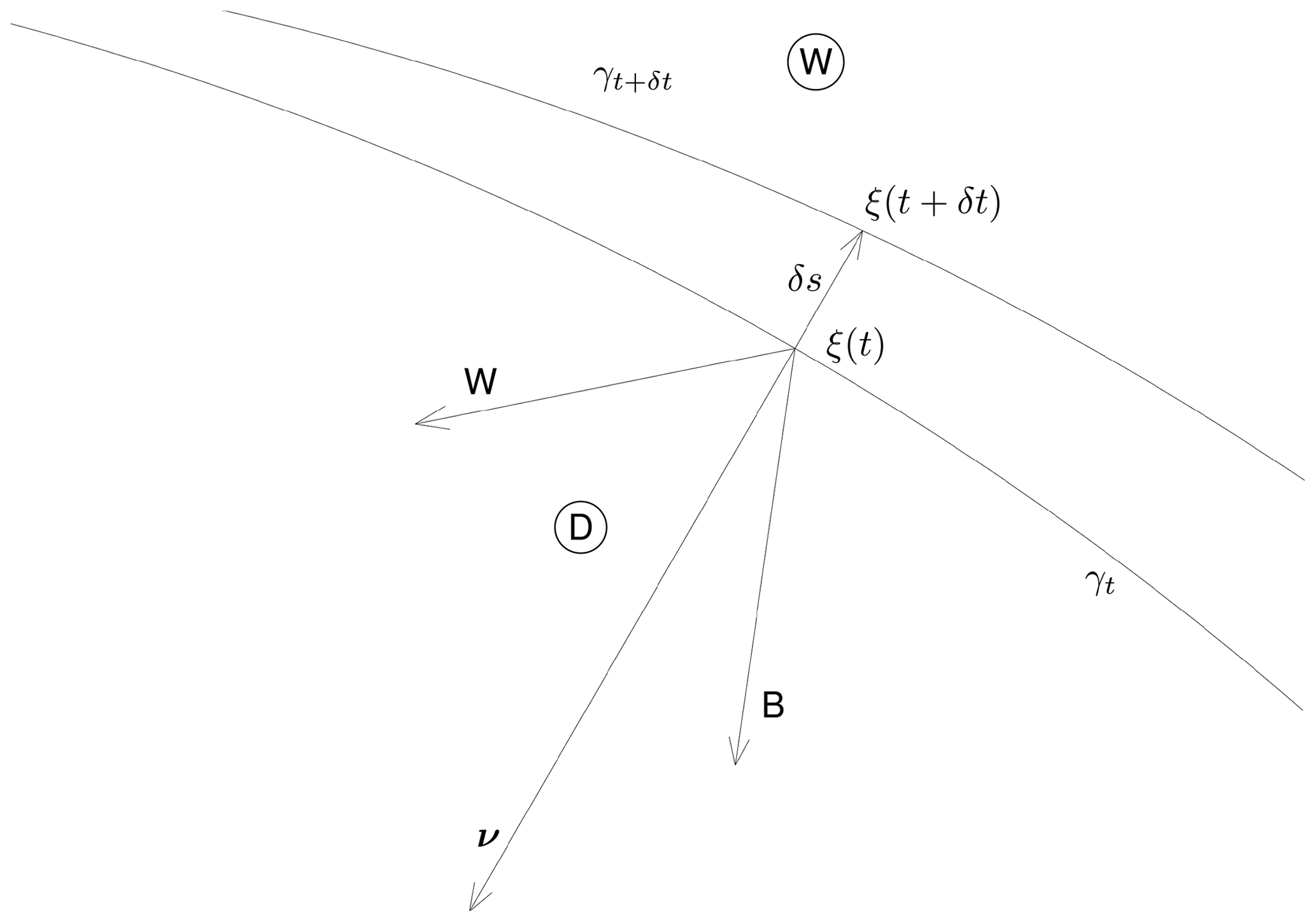
Figure 1 Evaporation front motion; W is the liquid water flux density and vapor advection in the gaseous phase, B is the water vapor flux density by diffusion in the gaseous phase, γ_t is the evaporation front position at time t, ν is the unit normal to the front pointing out of the wet zone, and ξ(t) is the position of a chosen point upon the front at time t.

The limit form of Eq. (11) for δt approaching zero gives

$$\begin{array}{}\text{(14)}& \begin{array}{rlr}& {\displaystyle \frac{\partial s}{\partial t}}(t,\mathit{\xi })& \\ & ={\displaystyle \frac{\begin{array}{c}\left(\mathit{\rho }\mathbf{w}\right(t,\mathit{\xi })+{\mathbf{b}}^{\mathrm{w}}(t,\mathit{\xi })+c^{\mathrm{w}}(t,\mathit{\xi }\left){\mathit{v}}^{\mathrm{w}}\right(t,\mathit{\xi })-{\mathbf{b}}^{\mathrm{d}}(t,\mathit{\xi })\\ -c^{\mathrm{d}}(t,\mathit{\xi }){\mathit{v}}^{\mathrm{d}}(t,\mathit{\xi }),\mathit{\nu }(t,\mathit{\xi }))\end{array}}{c^{\mathrm{w}}(t,\mathit{\xi })(n-\mathit{\theta }(t,\mathit{\xi }\left)\right)-n{c}^{\mathrm{d}}(t,\mathit{\xi })+\mathit{\rho }\mathit{\theta }(t,\mathit{\xi })}}.\end{array}\end{array}$$

By this equation and by the assumption of the direction of the front motion, we obtain the following ordinary first-order differential equation

$$\begin{array}{}\text{(15)}& \begin{array}{rl}& {\displaystyle \frac{\mathrm{d}\mathit{\xi }}{\mathrm{d}t}}\left(t\right)\\ & ={\displaystyle \frac{\begin{array}{c}\left(\mathit{\rho }\mathbf{w}\right(t,\mathit{\xi })+c^{\mathrm{w}}(t,\mathit{\xi }\left){\mathit{v}}^{\mathrm{w}}\right(t,\mathit{\xi })+{\mathbf{b}}^{\mathrm{w}}(t,\mathit{\xi })-{\mathbf{b}}^{\mathrm{d}}(t,\mathit{\xi })\\ -c^{\mathrm{d}}(t,\mathit{\xi }){\mathit{v}}^{\mathrm{d}}(t,\mathit{\xi }),\mathit{\nu }(t,\mathit{\xi }))\end{array}}{\begin{array}{c}{c}^{\mathrm{w}}(t,\mathit{\xi })(n-\mathit{\theta }(t,\mathit{\xi }\left)\right)-n{c}^{\mathrm{d}}(t,\mathit{\xi })\\ +\mathit{\rho }\mathit{\theta }(t,\mathit{\xi })\end{array}}}\mathit{\nu }(t,\mathit{\xi }).\end{array}\end{array}$$

Equation (15) is the governing equation of the evaporation front motion in the interval (0,T). The water density and porosity are presented as constants in Eqs. (11) and (15). Such an assumption is evidently not necessary, and the equations remain unchanged for $n=n(t,\mathit{\xi })$ and $\mathit{\rho }=\mathit{\rho }(t,\mathit{\xi })$.

In the cases we commonly meet in connection with problems of evaporation, the flow of the gaseous phase is restricted to balancing the changing volume of liquid water, i.e.,

$$\begin{array}{}\text{(16)}& \Vert \mathbf{w}\Vert \approx \Vert {\mathit{v}}^{\mathrm{d}}\Vert \approx \Vert {\mathit{v}}^{\mathrm{w}}\Vert ,\end{array}$$

and since

$$\begin{array}{}\text{(17)}& \mathit{\rho }\Vert \mathbf{w}\Vert \gg c^{\mathrm{d}}\Vert {\mathit{v}}^{\mathrm{d}}\Vert \mathrm{and}\mathit{\rho }\Vert \mathbf{w}\Vert \gg c^{\mathrm{w}}\Vert {\mathit{v}}^{\mathrm{w}}\Vert ,\end{array}$$

the advective transport of water vapor can be neglected. The governing equation becomes

$$\begin{array}{}\text{(18)}& \begin{array}{rl}& {\displaystyle \frac{\mathrm{d}\mathit{\xi }}{\mathrm{d}t}}\left(t\right)\\ & ={\displaystyle \frac{\left(\mathit{\rho }\mathbf{w}(t,\mathit{\xi })+{\mathbf{b}}^{\mathrm{w}}(t,\mathit{\xi })-{\mathbf{b}}^{\mathrm{d}}(t,\mathit{\xi }),\mathit{\nu }(t,\mathit{\xi })\right)}{c^{\mathrm{w}}(t,\mathit{\xi })(n-\mathit{\theta }(t,\mathit{\xi }\left)\right)-n{c}^{\mathrm{d}}(t,\mathit{\xi })+\mathit{\rho }\mathit{\theta }(t,\mathit{\xi })}}\mathit{\nu }(t,\mathit{\xi }).\end{array}\end{array}$$

3 Problem formulation

The front's motion reflects the proportions between the water flow and transport out of the front and towards the front which are given by the laws of flow and transport in the wet zone and in the dry zone. In order to evaluate flow and transport in porous media, Darcy's law and Fick's law can be utilized:

$$\begin{array}{}\text{(19)}& \begin{array}{rl}& \mathbf{w}=-k\left(h\right)\mathrm{grad}\left(x_{\mathrm{3}}+h\right),{\mathbf{b}}^{\mathrm{d}}=-D^{\mathrm{d}}\mathrm{grad}{c}^{\mathrm{d}},\\ & \mathrm{and}{\mathbf{b}}^{\mathrm{w}}=-D^{\mathrm{w}}\left(\mathit{\theta }\right)\mathrm{grad}{c}^{\mathrm{w}},\end{array}\end{array}$$

where the third coordinate x₃ is oriented vertically upwards, h is the pressure head, k is the hydraulic conductivity, and D^d and D^w are the coefficients of water diffusion in air within the porous medium.

In the dry zone, water is present in the form of water vapor, and its motion is governed by the continuity equation with the use of Fick's law:

$$\begin{array}{}\text{(20)}& {\displaystyle \frac{\partial }{\partial t}}\left(n{c}^{\mathrm{d}}\right)-{\displaystyle \frac{\partial }{\partial x_{\mathrm{i}}}}\left(D^{\mathrm{d}}{\displaystyle \frac{\partial c^{\mathrm{d}}}{\partial x_{\mathrm{i}}}}\right)+{\displaystyle \frac{\partial }{\partial x_{\mathrm{i}}}}\left(c^{\mathrm{d}}{v}_{\mathrm{i}}^{\mathrm{d}}\right)=\mathrm{0}.\end{array}$$

The vapor motion in the wet zone is governed by the same laws,

$$\begin{array}{}\text{(21)}& {\displaystyle \frac{\partial }{\partial t}}\left((n-\mathit{\theta })c^{\mathrm{w}}\right)-{\displaystyle \frac{\partial }{\partial x_{\mathrm{i}}}}\left(D^{\mathrm{w}}\left(\mathit{\theta }\right){\displaystyle \frac{\partial c^{\mathrm{w}}}{\partial x_{\mathrm{i}}}}\right)+{\displaystyle \frac{\partial }{\partial x_{\mathrm{i}}}}\left(c^{\mathrm{w}}{v}_{\mathrm{i}}^{\mathrm{w}}\right)=\mathrm{0},\end{array}$$

and the motion of liquid-phase water in the wet zone is governed by Richards' equation:

$$\begin{array}{}\text{(22)}& {\displaystyle \frac{\partial \mathit{\theta }}{\partial t}}-{\displaystyle \frac{\partial }{\partial x_{\mathrm{i}}}}\left(k\left(h\right)\left({\displaystyle \frac{\partial x_{\mathrm{3}}}{\partial x_{\mathrm{i}}}}+{\displaystyle \frac{\partial h}{\partial x_{\mathrm{i}}}}\right)\right)=\mathrm{0}.\end{array}$$

By virtue of the introduced theory, the evaporation front motion is governed by Eqs. (20), (21), (22) and (15) or (18). The unknown functions are θ and h, connected by the retention curve, c^w, c^d and ξ defined in $\stackrel{\mathrm{‾}}{G^{\mathrm{w}}}$, and $\stackrel{\mathrm{‾}}{G^{\mathrm{d}}}$ and [0,T). The functions $n,k,D,\mathit{v}$ and ρ are supposed to be known or given by additional equations.

In this way, Eqs. (21) and (22) in G^w and Eq. (20) in G^d stand for a coupled moving boundary problem, and Eq. (15) is a condition imposed upon the movable common part of the boundaries of the domains. The unknown function ξ defined in [0,T) is then given as the position of the moving boundary.

Another possible formulation of the problem is to solve the ordinary differential Eq. (15) in the interval [0,T), where the right-hand side of the equation is given as the solution of the Eqs. (21), (22) and (20) defined in G^w and G^d.

The latter approach was utilized when solving the problem presented in Sect. 5.

4 One-dimensional problem

Let now the studied domain be an interval Ω⊂ℝ¹:

$$\begin{array}{}\text{(23)}& \mathrm{\Omega }=(\mathrm{0},L),{\mathrm{\Omega }}_t^{\mathrm{w}}=(\mathrm{0},\mathit{\xi }(t\left)\right),{\mathrm{\Omega }}_t^{\mathrm{d}}=\left(\mathit{\xi }\right(t),L),\end{array}$$

where the function ξ(t) that denotes the position of the evaporation front at time t is a scalar function defined in (0,T). The sets G^w and G^d are

$$\begin{array}{}\text{(24)}& \begin{array}{rl}& G^{\mathrm{w}}=\mathit{\left\{}\right(t,x)\in {\mathbb{R}}^{\mathrm{2}};t\in (\mathrm{0},T),x\in (\mathrm{0},\mathit{\xi }\left(t\right)\left)\mathit{\right\}}\\ & \mathrm{and}{G}^{\mathrm{d}}=\mathit{\left\{}\right(t,x)\in {\mathbb{R}}^{\mathrm{2}};t\in (\mathrm{0},T),x\in (\mathit{\xi }\left(t\right),L\left)\mathit{\right\}}.\end{array}\end{array}$$

The image of the evaporation front in time–space is

$$\begin{array}{}\text{(25)}& \mathrm{\Gamma }=\mathit{\left\{}\right(t,x)\in {\mathbb{R}}^{\mathrm{2}};\mathit{\xi }(t)-x=\mathrm{0},t\in (\mathrm{0},T\left)\mathit{\right\}},\end{array}$$

and ν^Γ∈ℝ², the unit normal to Γ, is

$$\begin{array}{}\text{(26)}& {\mathit{\nu }}^{\mathrm{\Gamma }}(t,\mathit{\xi }(t\left)\right)=\left(-{\displaystyle \frac{\mathrm{d}\mathit{\xi }}{\mathrm{d}t}}\left(t\right),\mathrm{1}\right)/\sqrt{{\left({\displaystyle \frac{\mathrm{d}\mathit{\xi }}{\mathrm{d}t}}\left(t\right)\right)}^{\mathrm{2}}+\mathrm{1}}.\end{array}$$

The above-presented assertion concerning the direction of the evaporation front motion with respect to $\mathrm{sgn}\left({\mathit{\nu }}_t^{\mathrm{\Gamma }}\right)$ is now evident.

By virtue of the introduced theory, the law of the evaporation front motion is given by Eq. (15). In one space dimension, since ν(t,ξ) is either 1 or −1, the equation reads as

$$\begin{array}{}\text{(27)}& {\displaystyle \frac{\mathrm{d}\mathit{\xi }}{\mathrm{d}t}}\left(t\right)={\displaystyle \frac{\begin{array}{c}\mathit{\rho }w(t,\mathit{\xi })+c^{\mathrm{w}}(t,\mathit{\xi })v^{\mathrm{w}}(t,\mathit{\xi })+b^{\mathrm{w}}(t,\mathit{\xi })\\ -b^{\mathrm{d}}(t,\mathit{\xi })-c^{\mathrm{d}}(t,\mathit{\xi })v^{\mathrm{d}}(t,\mathit{\xi })\end{array}}{c^{\mathrm{w}}(t,\mathit{\xi })(n-\mathit{\theta }(t,\mathit{\xi }\left)\right)-n{c}^{\mathrm{d}}(t,\mathit{\xi })+\mathit{\rho }\mathit{\theta }(t,\mathit{\xi })}}\end{array}$$

and its simplified form (18) is

$$\begin{array}{}\text{(28)}& {\displaystyle \frac{\mathrm{d}\mathit{\xi }}{\mathrm{d}t}}\left(t\right)={\displaystyle \frac{\mathit{\rho }w(t,\mathit{\xi })+b^{\mathrm{w}}(t,\mathit{\xi })-b^{\mathrm{d}}(t,\mathit{\xi })}{c^{\mathrm{w}}(t,\mathit{\xi })(n-\mathit{\theta }(t,\mathit{\xi }\left)\right)-n{c}^{\mathrm{d}}(t,\mathit{\xi })+\mathit{\rho }\mathit{\theta }(t,\mathit{\xi })}}.\end{array}$$

In order to complete the problem formulation, to determine the right-hand-side function, the one-dimensional form of Eqs. (18) to (22) can be utilized.

5 A solved problem

In the framework of wider research that concerns evaporation from rock surfaces and the time dependence of evaporation front positions, an experiment was carried out. It was an unpublished auxiliary experiment performed by several of the author's colleagues, and since it was not sufficiently documented from the point of view of this study, it cannot be simulated. Nevertheless, part of its results can be utilized here in order to present an example of possible use of the achieved theoretical results. The missing data were simply chosen, not optimized. The following description should be understood as a problem formulation, not as a documentation of measurements.

A cylinder-shaped sample of the studied rock was put into position with the horizontal axis. The jacket of the cylinder was insulated so that no water (of any phase) could penetrate, and the motion of water through the sample was possible only in the horizontal direction along the cylinder's axis.

The length of the sample was L=49 mm, and the length of the time interval was T=63 d. One open end of the sample, say x=0, was equipped so that it was possible to measure the pressure head and the rate of water inflow into the sample at this point. The obtained discrete data were approximated by smooth functions h₀(t) and w₀(t) (pressure head and volumetric flux density), $h_{\mathrm{0}},w_{\mathrm{0}}\in C^{\mathrm{1}}(\mathrm{0},T)$, that were utilized as the imposed boundary conditions.

Figure 2 shows the pressure head values; the squares are the measured data, and the solid curve is their approximation h₀.

Figure 2 The x=0 boundary condition – the pressure head at the boundary. The squares show the measured values, and the smooth function is their approximation h₀(t) that was used in the solved example.

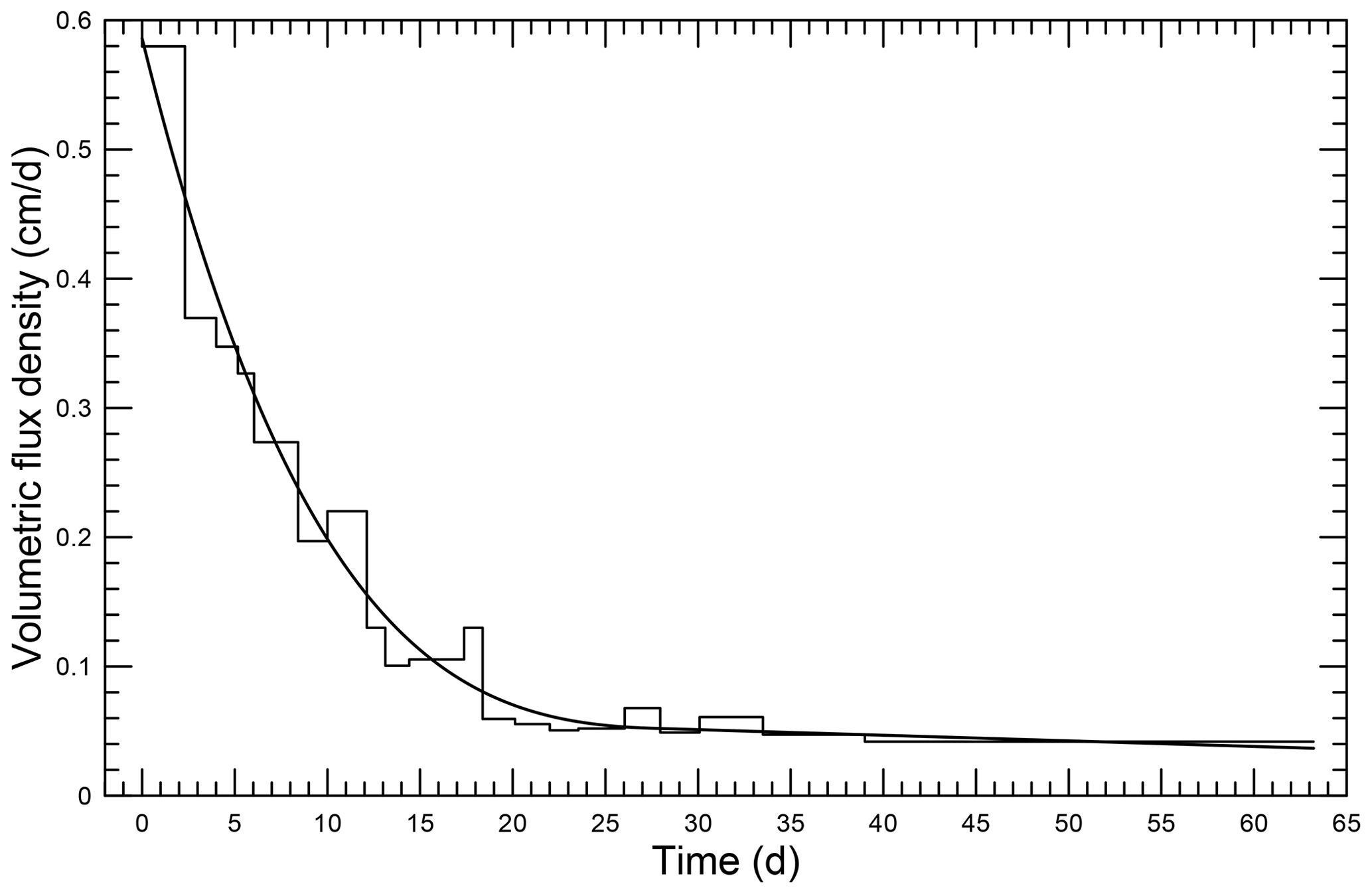
Figure 3 The x=0 boundary condition – the volumetric flux density at the boundary. The step function shows the measured values, and the smooth function is its approximation used in the solved example.

The volumetric flux density was measured indirectly in the form of discrete values of the cumulative flux to the sample. In Fig. 3, the step function represents the measured data and the smooth function is the boundary condition w₀. The integral values over (0,T) (the total inflow to the sample per unit surface) of both functions are equal. The other end of the sample, x=L, was left open to the outer (atmospheric) conditions which were not measured.

Soil moisture retention data and the hydraulic conductivity (at saturation) K_s were obtained elsewhere using samples of similar material. Making use of these characteristics, the Mualem and van Genuchten parameters ${\mathit{\theta }}_{\mathrm{r}},{\mathit{\theta }}_{\mathrm{s}},\mathit{\alpha },m$ and n were determined and, hence, the hydraulic conductivity and the soil moisture retention curve as functions of either pressure head or water content were defined.

Similarly, the value of the diffusion coefficient of water in the gaseous phase within the porous medium, D^d, was obtained measured on samples of the utilized material. The characteristic surface layer ε was added from outside to the domain Ω, and its value was taken from the paper of Slavík et al. (2020), where the layer is referred to as “calibrated L” and also as “boundary layer”.

The fluorescein visualization method (Weiss et al., 2018) was utilized to detect the front's position during the experiment. Fluorescein was applied at the water input side of the sample, and a set of couples (t,ξ), time and the front's position was registered. The data were calibrated (using a simple linear transformation) to agree with the value measured after finishing the experiment.

The following problem was formulated. In the interval [0,T], the solution t↦ξ(t), $\mathit{\xi }\in C^{\mathrm{1}}(\mathrm{0},T)\cap C[\mathrm{0},T]$, of Eq. (28) is sought that satisfies the initial condition

$$\begin{array}{}\text{(29)}& \mathit{\xi }\left(\mathrm{0}\right)=L,\end{array}$$

where ρ and n (density and porosity) are known constants.

Since neither functions c^d and c^w nor their boundary values at $x=\mathrm{0},\mathit{\xi }\left(t\right)$ and L were measured during the experiment, the following two assumptions were introduced.

(^*) The vapor concentration has a constant value c_f at the evaporation front in the gaseous phase and at points of positive value of water content θ, i.e., at points of contact with liquid-phase water.

(${}^{**}$) There are steady-state outer atmospheric conditions during the process giving a constant value c_e of vapor concentration in the gaseous phase at x=L.

The assumptions do not contradict each other at the point ξ(0), since the characteristic surface layer ε was accepted in the model. As presented above, the right-hand side of Eq. (28) can be determined by solving the related initial boundary value problems with Eqs. (20), (21), and (22).

In view of assumption (^*) and Eqs. (21) and (19), it holds that

$$\begin{array}{}\text{(30)}& c^{\mathrm{w}}(t,x)=c_{\mathrm{f}}\mathrm{and}{b}^{\mathrm{w}}(t,x)=\mathrm{0}\mathrm{in}{G}^{\mathrm{w}}.\end{array}$$

Applying assumption (^*), Eq. (21) reads as

$$\begin{array}{}\text{(31)}& {\displaystyle \frac{\partial \mathit{\theta }}{\partial t}}-{\displaystyle \frac{\partial v^{\mathrm{w}}}{\partial x}}=\mathrm{0}.\end{array}$$

The comparison with Richards' Eq. (22) gives $v^{\mathrm{w}}=-w$; the gaseous phase continuously replaces the leaving water. A similar result has already been expected even for more general cases; see the estimations utilized when replacing Eq. (15) by Eq. (18). Making use of these results, Eq. (28) becomes

$$\begin{array}{}\text{(32)}& {\displaystyle \frac{\mathrm{d}\mathit{\xi }}{\mathrm{d}t}}\left(t\right)={\displaystyle \frac{\mathit{\rho }w(t,\mathit{\xi })-b(t,\mathit{\xi })}{\mathit{\theta }(t,\mathit{\xi })(\mathit{\rho }-c_{\mathrm{f}})}},\end{array}$$

where the unknown parameters on the right-hand side of Eq. (32) are solutions of the following two initial boundary value problems and, since b^w, c^w and D^w do not appear in what follows, b, c and D stand for b^d, c^d and D^d.

To determine functions θ and w, function h defined in G^w is sought that satisfies Eq. (22), now in the form

$$\begin{array}{}\text{(33)}& {\displaystyle \frac{\partial \mathit{\theta }}{\partial t}}-{\displaystyle \frac{\partial }{\partial x}}\left(k\left(h\right){\displaystyle \frac{\partial h}{\partial x}}\right)=\mathrm{0}\end{array}$$

and the conditions

$$\begin{array}{}\text{(34)}& h(\mathrm{0},x)=h_{\mathrm{i}}\left(x\right)\mathrm{in}(\mathrm{0},L)\end{array}$$

and

$$\begin{array}{}\text{(35)}& \begin{array}{rl}& h(t,\mathrm{0})=h_{\mathrm{0}}\left(t\right)\\ & \mathrm{and}-k\left(h\right(t,\mathrm{0}\left)\right){\displaystyle \frac{\partial h}{\partial x}}(t,\mathrm{0})=w_{\mathrm{0}}\left(t\right)\mathrm{in}(\mathrm{0},T),\end{array}\end{array}$$

where θ(h) is the retention curve. Functions h₀ and w₀ are known from the experiment, and function h_i, the initial pressure head distribution, was not measured and has to be determined.

Incorporating the characteristic surface layer into the problem formulation, we change the set G^d to

$$\begin{array}{}\text{(36)}& G^{\mathrm{d}}=\mathit{\left\{}\right(t,x)\in {\mathbb{R}}^{\mathrm{2}};x\in (\mathit{\xi }\left(t\right),L+\mathit{\epsilon }),t\in (\mathrm{0},T\left)\mathit{\right\}}.\end{array}$$

Now, c solves the equation

$$\begin{array}{}\text{(37)}& {\displaystyle \frac{\partial }{\partial t}}\left(nc\right)-{\displaystyle \frac{\partial }{\partial x}}\left(D{\displaystyle \frac{\partial c}{\partial x}}\right)=\mathrm{0}\end{array}$$

in G^d and satisfies the conditions

$$\begin{array}{}\text{(38)}& c(\mathrm{0},x)=c_{\mathrm{i}}\left(x\right)\mathrm{in}(L,L+\mathit{\epsilon })\end{array}$$

and

$$\begin{array}{}\text{(39)}& c(t,\mathit{\xi }(t\left)\right)=c_{\mathrm{f}}\mathrm{and}c(t,L+\mathit{\epsilon })=c_{\mathrm{e}}\mathrm{in}(\mathrm{0},T),\end{array}$$

where c_i is the initial distribution of the water concentration in the gaseous phase. The values c_e and c_f were chosen with respect to these requirements: the relative humidity at the front was 100 %, the outer relative humidity was between 30 % and 50 % and the temperature was between 18 and 23 ^∘C.

In order to define the initial state of the sample, functions c_i and h_i, it was assumed that the process started from the steady-state water vapor diffusion determined in $(L,L+\mathit{\epsilon })$ by the boundary values c_f and c_e and from the steady-state water flow determined in (0,L) by the initial conditions h₀(0) and w₀(0). The error involved in functions c_i and h_i vanishes soon, since the sample is small and the imposed boundary conditions take over the dominant role.

Our requirement for the initial conditions is easy to satisfy in the case of function c_i in the domain ${\mathrm{\Omega }}_{t=\mathrm{0}}^{\mathrm{d}}$, since, in view of Eq. (37), the governing equation is

$$\begin{array}{}\text{(40)}& {\displaystyle \frac{\mathrm{d}}{\mathrm{d}x}}\left(D{\displaystyle \frac{\mathrm{d}{c}_{\mathrm{i}}}{\mathrm{d}x}}\right)=\mathrm{0}\mathrm{in}(L,L+\mathit{\epsilon }).\end{array}$$

With respect to the boundary conditions, the solution reads as

$$\begin{array}{}\text{(41)}& c_{\mathrm{i}}\left(x\right)={\displaystyle \frac{c_{\mathrm{e}}-c_{\mathrm{f}}}{\mathit{\epsilon }}}(x-L)+c_{\mathrm{f}}.\end{array}$$

In the case of function h_i and domain ${\mathrm{\Omega }}_{t=\mathrm{0}}^{\mathrm{w}}$, the governing equation is

$$\begin{array}{}\text{(42)}& {\displaystyle \frac{\mathrm{d}}{\mathrm{d}x}}\left(\mathit{\rho }k\left(h_{\mathrm{i}}\right){\displaystyle \frac{\mathrm{d}{h}_{\mathrm{i}}}{\mathrm{d}x}}\right)=\mathrm{0}\mathrm{in}(\mathrm{0},L),\end{array}$$

with the initial conditions

$$\begin{array}{}\text{(43)}& h_{\mathrm{i}}\left(\mathrm{0}\right)=h_{\mathrm{0}}\left(\mathrm{0}\right)\mathrm{and}-k\left(h_{\mathrm{i}}\right(\mathrm{0}\left)\right){\displaystyle \frac{\mathrm{d}{h}_{\mathrm{i}}}{\mathrm{d}x}}\left(\mathrm{0}\right)=w_{\mathrm{0}}\left(\mathrm{0}\right).\end{array}$$

The solution to the problem (42), (43), is equivalent to the solution to the problem

$$\begin{array}{}\text{(44)}& {\displaystyle \frac{\mathrm{d}{h}_{\mathrm{i}}}{\mathrm{d}x}}=-{\displaystyle \frac{w_{\mathrm{0}}\left(\mathrm{0}\right)}{k\left(h_{\mathrm{i}}\right)}}\mathrm{in}(\mathrm{0},L),\end{array}$$

with the initial condition h_i(0)=h₀(0). Let the maximum solution to this initial value problem be defined in [0,λ). It can be shown that, in our case, λ>L and the wet zone reach the point x=L. Hence, our choice of the initial condition h_i does not contradict the initial condition (29).

Now the problem (32), (29), can be solved numerically. The utilized values are the Mualem and van Genuchten parameters α=0.0223 cm⁻¹, n=1.99, and $m=\mathrm{1}-\mathrm{1}/n$, the saturated hydraulic conductivity K_s=0.0071 cm s⁻¹ and the diffusion coefficient of water in the gaseous phase within the porous medium D^d=0.045 cm² s⁻¹. Figure 4 shows three solutions obtained for three different couples of chosen parameters and the boundary values of water concentration in the gaseous phase. The chosen values were

• (1)

  $c_{\mathrm{f}}=\mathrm{2.27}\times {\mathrm{10}}^{-\mathrm{5}}$ g/cm³, $c_{\mathrm{e}}=\mathrm{9.35}\times {\mathrm{10}}^{-\mathrm{6}}$ g/cm³,

• (2)

  $c_{\mathrm{f}}=\mathrm{2.41}\times {\mathrm{10}}^{-\mathrm{5}}$ g/cm³, $c_{\mathrm{e}}=\mathrm{9.94}\times {\mathrm{10}}^{-\mathrm{6}}$ g/cm³,

• (3)

  $c_{\mathrm{f}}=\mathrm{2.56}\times {\mathrm{10}}^{-\mathrm{5}}$ g/cm³, $c_{\mathrm{e}}=\mathrm{1.06}\times {\mathrm{10}}^{-\mathrm{5}}$ g/cm³.

When using the method by McRae (1980) and choosing the relative humidity at the evaporation front and at the sample's surface as 100 % and 40 %, respectively, we get the following temperatures at the evaporation front and at the sample's surface: (1) 19.5 ^∘C and 20.0 ^∘C, (2) 20.5 ^∘C and 21.0 ^∘C, and (3) 21.5 ^∘C and 22.0 ^∘C.

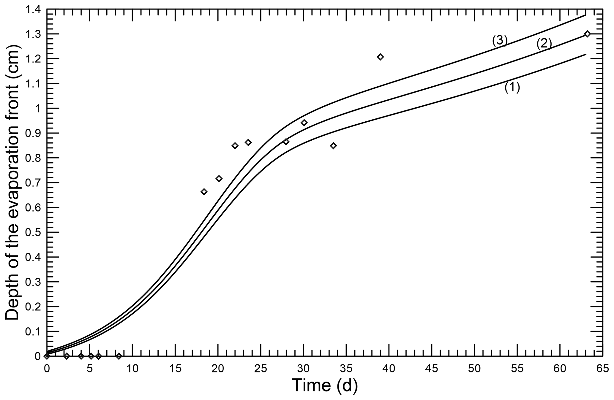
Figure 4 Evaporation front motion. ⋄: measured positions, solid lines: numerical simulations. (1) $c_{\mathrm{f}}=\mathrm{2.27}\times {\mathrm{10}}^{-\mathrm{5}},c_{\mathrm{e}}=\mathrm{9.35}\times {\mathrm{10}}^{-\mathrm{6}},$ (2) $c_{\mathrm{f}}=\mathrm{2.41}\times {\mathrm{10}}^{-\mathrm{5}},c_{\mathrm{e}}=\mathrm{9.94}\times {\mathrm{10}}^{-\mathrm{6}},$ (3) $c_{\mathrm{f}}=\mathrm{2.56}\times {\mathrm{10}}^{-\mathrm{5}},c_{\mathrm{e}}=\mathrm{1.06}\times {\mathrm{10}}^{-\mathrm{5}}$, all in grams per cubic centimeter.

The problem (32), (29), was solved numerically using a predictor–corrector method. The values of the right-hand side were determined using the method of Rothe to solve problems (33) to (35) and (37) to (39).

Let M_w denote the total mass of liquid water in the investigated domain related to the unit cross section. Then it holds that

$$\begin{array}{}\text{(45)}& M_{\mathrm{w}}\left(t\right)=\underset{\mathrm{0}}{\overset{\mathit{\xi }\left(t\right)}{\int }}\mathit{\rho }\mathit{\theta }(t,x)\mathrm{d}x.\end{array}$$

Hence, the rate of its change is

$$\begin{array}{}\text{(46)}& {\displaystyle \frac{\mathrm{d}{M}_{\mathrm{w}}}{\mathrm{d}t}}\left(t\right)=\mathit{\rho }{\displaystyle \frac{\mathrm{d}\mathit{\xi }}{\mathrm{d}t}}\left(t\right)\mathit{\theta }(t,\mathit{\xi }(t\left)\right)+\mathit{\rho }\underset{\mathrm{0}}{\overset{\mathit{\xi }\left(t\right)}{\int }}{\displaystyle \frac{\partial \mathit{\theta }}{\partial t}}(t,x)\mathrm{d}x.\end{array}$$

Making use of Eqs. (32), (33) and (19), we get

$$\begin{array}{}\text{(47)}& \begin{array}{rl}{\displaystyle \frac{\mathrm{d}{M}_{\mathrm{w}}}{\mathrm{d}t}}\left(t\right)& =\mathit{\rho }{\displaystyle \frac{\mathit{\rho }w(t,\mathit{\xi }(t\left)\right)-b(t,\mathit{\xi }(t\left)\right)}{\mathit{\rho }-c_{\mathrm{f}}}}\\ & +\mathit{\rho }\left(w(t,\mathrm{0})-w(t,\mathit{\xi }(t\left)\right)\right).\end{array}\end{array}$$

Since ρ w(t,0) is the inflow of liquid water into the domain,

$$\begin{array}{}\text{(48)}& E\left(t\right)={\displaystyle \frac{b(t,\mathit{\xi }(t\left)\right)-c_{\mathrm{f}}w(t,\mathit{\xi }(t\left)\right)}{\mathrm{1}-c_{\mathrm{f}}/\mathit{\rho }}}\end{array}$$

is, under the assumptions of this section, the rate of evaporation expressed as the mass of evaporated water per unit time and unit surface of the evaporation front. Consequently, having solved an evaporation front motion problem, the demands of the latent heat of vaporization can be evaluated and located in time and space.

6 Discussion and conclusions

The evaporation front has been defined as an interface separating two different zones, wet and dry, inside or upon the boundary of a porous-medium domain. The exact definition of these zones, presented in this paper, is based on the form of water they contain. Subsequently, the law of the evaporation front motion was formulated in the form of the vector Eq. (15). Since the law is based on the complete mass balance of water, i.e., liquid water and water vapor, it holds generally and does not need any additional account of energy. The laws of heat transfer and heat balance do not affect the presented equations which define the evaporation front motion. On the contrary, solving problems that are fully determined by water transport data, the equations of the evaporation front motion can give certain insight into the energy requirements of such processes, e.g., the final part of Sect. 5.

Smits et al. (2011) and Nuske et al. (2014) studied the process of evaporation from soils with particular attention to the phase change and found that nonequilibrium models yield better agreement with experimental data than equilibrium models. The nature of the phase change process does not affect the results presented here directly, since the equation of the evaporation front motion requires other kinds of data. The process of phase change enters Eq. (15) through its actual effect on the transport of water. On the other hand, the constitution laws like Darcy's law or the retention curve that may be utilized when solving problems with Eq. (15) are equilibrium laws. In the example presented in Sect. 5, equilibrium laws were utilized. However, the governing Eq. (15), being general, makes it possible to use nonequilibrium laws as well. Mls (1999) presented a general nonequilibrium approach to two-phase systems that keeps Darcy's law valid.

Lehmann et al. (2008) and Or et al. (2013) investigated the process of evaporation from the top of an initially saturated vertical column. They introduced the term “characteristic length” as the distance between the surface and the receding drying front (interface between the saturated zone and the unsaturated zone) and described different stages of the evaporation process. No evaporation front was introduced. By virtue of the present theory, the evaporation front cannot move in the positive direction of ν(t,ξ) if

$$\begin{array}{}\text{(49)}& \mathit{\xi }\left(t\right)\in \stackrel{\mathrm{‾}}{{\mathrm{\Omega }}_t^{\mathrm{w}}}\cap B_t^{\mathrm{d}},\end{array}$$

i.e., if ξ(t) is a point of a “dry-from-outside” part of the domain boundary. Hence, see Eq. (14): the front does not move until the condition

$$\begin{array}{}\text{(50)}& \begin{array}{rl}\left(\right(\mathit{\rho }\mathbf{w}(t,\mathit{\xi })& +c^{\mathrm{w}}(t,\mathit{\xi }){\mathit{v}}^{\mathrm{w}}(t,\mathit{\xi })+{\mathbf{b}}^{\mathrm{w}}(t,\mathit{\xi })-{\mathbf{b}}^{\mathrm{d}}(t,\mathit{\xi })\\ & -c^{\mathrm{d}}(t,\mathit{\xi }){\mathit{v}}^{\mathrm{d}}(t,\mathit{\xi })),\mathit{\nu }(t,\mathit{\xi }\left)\right)<\mathrm{0}\end{array}\end{array}$$

is satisfied. In the simplified one-dimensional case, Eq. (28), this condition reads as

$$\begin{array}{}\text{(51)}& \left(\mathit{\rho }w(t,\mathit{\xi })+b^{\mathrm{w}}(t,\mathit{\xi })-b^{\mathrm{d}}(t,\mathit{\xi })\right)\mathit{\nu }(t,\mathit{\xi })<\mathrm{0},\end{array}$$

where $\mathit{\nu }(t,\mathit{\xi })=\mathrm{1}$ if $x\in {\mathrm{\Omega }}_t^{\mathrm{w}}\Rightarrow x<\mathit{\xi }\left(t\right)$ and vice versa. Under conditions of sufficiently small values of $\left|b^{\mathrm{d}}\right|$, condition (51) is not satisfied for a period, and the evaporation front does not move. Consequently, the evaporation rate does not change significantly. In the solved problem, the chosen initial conditions and the size of ε make Eq. (51) valid even at t=0, and the front moves from the very beginning of the process. If the flux density of liquid water from inside of the wet zone exceeds the flux density b(t,L), either θ(t,L) increases or, being $\mathit{\theta }(t,L)={\mathit{\theta }}_{\mathrm{sat}}$, flux density $\mathit{\rho }w(t,L)-b(t,L)$ of liquid water discharges out of the porous-medium domain.

The characteristic surface layer ε was found experimentally, see Slavík et al. (2020), and accepted in this paper as a part of the measured data. Note that Song et al. (2018) studied similar problems and also introduced a special diffusion layer outside the porous medium. From the viewpoint of moving front equations, the characteristic surface layer prevents infinite values of function b^d at x=0 and t=0 which may be obtained when solving a problem with Eq. (20). This possibility originates in the fact that the equation is a balance equation that contains an equilibrium law – Fick's law; for more on this problem and an alternate approach, see Mls and Herrmann (2011).

The process of evaporation alone does not determine the direction of the evaporation front motion. Since the denominator of the right-hand side of Eq. (15) is positive, the direction of the evaporation front motion is determined by the sign of the scalar product in the numerator. Consequently, both the processes of wetting or drying (increasing or decreasing the wet zone) can take place while evaporating water out of the profile; compare also Eqs. (32) and (48).

The presented problem example and its numerical solutions were aimed at showing the ability of the theory to simulate real processes, not at getting an optimized agreement. Most of the measured parameters of the solved problem were obtained independently of the experiment. Only the pressure head and water flow data shown in Figs. 2 and 3 were measured during the experiment and utilized as the imposed boundary conditions of the problem. The concentration of water in the gaseous phase, the functions c_f and c_e, and the initial values of functions h and w were not measured but chosen. For the sake of their simple interpretation by means of acceptable values of temperatures and relative humidities, c_f and c_e were kept constant. No method of fitting was applied, and a different choice of functions h_i and w_i and constants c_e and c_f can give a better agreement between the measured and computed values.

The presented theory is now prepared to prove its reliability in such problems that are fully documented and to be used when solving a wide range of problems of evaporation from a rock or soil profile.