the Creative Commons Attribution 4.0 License.
the Creative Commons Attribution 4.0 License.
 | 14 Jul 2022
A novel objective function DYNO for automatic multivariable calibration of 3D lake models
Taimoor Akhtar
Christine A. Shoemaker
This study introduced a novel Dynamically Normalized Objective Function (DYNO) for multivariable (i.e., temperature and velocity) model calibration problems. DYNO combines the error metrics of multiple variables into a single objective function by dynamically normalizing each variable's error terms using information available during the search. DYNO is proposed to dynamically adjust the weight of the error of each variable hence balancing the calibration to each variable during optimization search. DYNO is applied to calibrate a tropical hydrodynamic model where temperature and velocity observation data are used for model calibration simultaneously. We also investigated the efficiency of DYNO by comparing the calibration results obtained with DYNO with the results obtained through calibrating to temperature only and with the results obtained through calibrating to velocity only. The results indicate that DYNO can balance the calibration in terms of water temperature and velocity and that calibrating to only one variable (e.g., temperature or velocity) cannot guarantee the goodness-of-fit of another variable (e.g., velocity or temperature) in our case. Our study implies that in practical application, for an accurate spatially distributed hydrodynamic quantification, including direct velocity measurements is likely to be more effective than using only temperature measurements for calibrating a 3D hydrodynamic model. Our example problems were computed with a parallel optimization method PODS, but DYNO can also be easily used in serial applications.
- Article
(9357 KB) - Full-text XML
-
Supplement
(1279 KB) - BibTeX
- EndNote


Lake hydrodynamic models simulate the hydrodynamic or thermodynamic processes in lakes and reservoirs that are important for simulating water quality in aquatic ecosystems (Chanudet et al., 2012). These simulation models (e.g., hydrodynamic modeling) play a critical role in managing water bodies, as they are built to support the simulation of the spatial and temporal distributions of specific water quality variables (e.g., nutrients, chlorophyll a), and to study the response of a water body to different future management scenarios. The parameters of these models usually need to be calibrated to measured data in order to adequately represent local effects and hydrodynamic processes. Model calibration is a vital step in complex hydrodynamic modeling of lakes and other aquatic systems.
Model calibration of lake hydrodynamic models is mainly done manually (also called “trial and error”), where experts tune the parameters and simultaneously evaluate the goodness-of-fit between the simulation output and observations. This process is subjective, time-intensive, and requires extensive expert knowledge (Afshar et al., 2011; Xia et al., 2021; Solomatine et al., 1999; Fabio et al., 2010; Baracchini et al., 2020). The challenges associated with manual calibration have encouraged the application of auto-calibration to lake hydrodynamic models, where the calibration is set up as an inverse problem to minimize the error between the simulation and observations. Some studies (e.g., Gaudard et al., 2017, Luo et al., 2018, Ayala et al., 2020 and Wilson et al., 2020) have applied automatic calibration to one-dimensional (1D) hydrodynamic lake models where water temperature is the variable that is simulated and calibrated. These 1D models are relatively cheap to run, enabling the use of automatic calibration methods that typically require many simulation evaluations to determine suitable parameter sets (e.g., differential evolution used in Luo et al., 2018 and Monte Carlo sampling used in Ayala et al., 2020). However, 1D models are unable to simulate the horizontal spatial distribution and cannot capture the 3D processes, and thus may not be suitable for certain studies. Consequently, 2D or 3D models are preferred for studying the spatial–temporal distribution of water variables and are increasingly used to study lakes around the world (Chanudet et al., 2012; Galelli et al., 2015; Hui et al., 2018; Soulignac et al., 2017; Wahl and Peeters, 2014; Xu et al., 2017; Baracchini et al., 2020). The calibration of 3D models, however, is considerably more challenging than calibration of 1D models, since 3D models are significantly more expensive computationally and they also involve more complicated physical processes (such as advection of flows).
The computationally expensive character of 3D lake models makes traditional optimization methods, such as differential evolution and Monte Carlo sampling, unsuitable for automatic calibration because these methods usually require many evaluations to get an acceptable solution. Surrogate-based optimization is highly suitable for such problems (Bartz-Beielstein and Zaefferer, 2017; Lu et al., 2018; Razavi et al., 2012) and recent studies have applied surrogate-based optimization methods to parameter estimation of hydrodynamics models. Surrogate-based optimization methods use a cheap-to-run surrogate approximation model (of the calibration objective) fitted with all known (i.e., already evaluated) values of the original expensive objective function, to guide the optimization search and reduce the number of evaluations required on the expensive simulations. For example, Xia et al. (2021) proposed a new optimization method called PODS (parallel optimization with dynamic coordinate search using surrogates) suitable for computationally expensive problems, and applied it to automatic calibration of 3D hydrodynamic lake models. More elaborate discussions on surrogate-based optimization algorithms can be found in Xia et al. (2021), Xia and Shoemaker (2021), Razavi et al. (2012), Bartz-Beielstein and Zaefferer (2017), and Haftka et al. (2016).
Computational intensity is not the only critical challenge associated with parameter estimation of 3D hydrodynamic lake models. Parameter estimation of these models is also a multisite and multivariable calibration problem, i.e., observation data are usually available at multiple locations and the underlying models simulate multiple variables (e.g., temperature and velocity). Moreover, simultaneous calibration of multiple variables is desired due to complex interactions between the different variables. For instance, temperature and velocity are interdependent variables of a hydrodynamic lake model, since water temperature affects the movement of water, and water velocity affects the distribution of water temperature. However, most prior research studies have calibrated hydrodynamic models to only temperature. This might be because temperature measurements are relatively less expensive to obtain compared with velocity measurements, and often temperature measurements are available to help predict water quality phenomena. Wahl and Peeters (2014) use the measured water temperatures to calibrate a 3D hydrodynamic model of Lake Constance. Kaçýkoç and Beyhan (2014) calibrate the temperature of Lake Egirdir with a hydrodynamic model, the flow simulation of which is used for modeling of the lake water quality. Marti et al. (2011) and Xue et al. (2015) also only used temperature data for calibration of hydrodynamic lake models. Moreover, these studies use manual calibration for parameter estimation. Xia et al. (2021) use automatic calibration for parameter estimation, but they only use water temperature observations in the calibration process. Reproducing the water level is also a parameter estimation approach that pseudo-considers flow dynamics in calibration; however, a calibrated model that correctly simulates the observed water level does not necessarily reproduce the observed 3D flow field accurately (Wagner and Mueller, 2002; Parsapour-Moghaddam and Rennie, 2018). Amadori et al. (2021) investigated the use of different sources of temperature data (from in-suite observations, multisite high-resolution profiles, and remote sensing data) to compensate for the scarcity of velocity measurements. This is a practicable approach when there are no velocity data available and there are such different sources of temperature data available. However, when there are no high-quality remote sensing data (e.g., because of cloud) or a large amount of high-resolution profiles of temperature measurements, it is still challenging to verify the spatial simulation of hydrodynamic quantities.
Hydrodynamic lake models predict the velocities throughout a water body. Accurate velocity simulations are thus important for understanding the spatial distribution of water quality problems (e.g., algal blooms) in sizeable lakes. Hence, during the calibration of these models, it is useful to know whether efforts to measure velocity directly are justifiable even if temperature data are already available. We will examine the extent to which direct measurement of velocities justifies the extra effort by giving more accurate results for hydrodynamics models. We will also look at the error of the spatial distribution of hydrodynamics associated with calibrating to temperature only, which is rarely studied in the literature.
There are a few studies that attempt to calibrate hydrodynamic lake models to both temperature and velocity. Chanudet et al. (2012) attempted to calibrate both temperature and velocity sequentially (using manual calibration), i.e., they calibrate water temperature first and then the current velocities. Baracchini et al. (2020) performed two sequential steps in the automatic calibration of temperature and velocity, and the velocity calibration is based on the results obtained from temperature calibration. However, one problem with such two-step sequential approaches, either by manual or auto-calibration, is that the calibration of the second variable might significantly alter the calibration quality of the first variable. This is especially true for multivariable calibration problems, where the multiple variables being calibrated are sensitive to the parameters being calibrated. Other examples of such multivariable calibration problems include watershed model calibration (Franco et al., 2020) and seawater intrusion model calibration (Coulon et al., 2021), among others. These multivariable problems require calibration frameworks that enable the simultaneous calibration of all variables rather than calibrating one variable and then the second.
There are studies that simultaneously calibrate both temperature and velocity variables of hydrodynamic models. However, these use a trial-and-error (manual) mechanism for calibration (Råman Vinnå et al., 2017; Soulignac et al., 2017; Jin et al., 2000; Paturi et al., 2014). Manual calibration of multiple hydrodynamic variables simultaneously is even harder than calibration of a single variable. A key challenge for automatic calibration of multivariable calibration problems is in defining a suitable objective function. Traditional approaches typically formulate the goodness-of-fit of multiple variables into a single objective function by adding weights between the goodness-of-fit of multiple variables and solve the problem with single objective optimization (SOO) techniques (Afshar et al., 2011; Pelletier et al., 2006). However, a drawback of this approach is that the relative error magnitude of each variable of the new solutions found will probably vary during the search, making it difficult to determine appropriate weights since they need to be determined or defined a priori, i.e., before optimization.
Another approach for calibration of multivariables is using multiobjective optimization (MOO) techniques (Afshar et al., 2013). However, multiobjective techniques are commonly used to optimize multiple sub-objectives that have a trade-off between each sub-objective (Akhtar and Shoemaker, 2016; Reed et al., 2013; Alfonso et al., 2010; Giuliani et al., 2016; Herman et al., 2014). For the multivariable hydrodynamic calibration problems, however, it is not apparent that there is usually a trade-off between the fit of multiple variables. Moreover, MOO is considerably more computationally difficult than SOO and typically requires many more objective function evaluations. Thus, MOO may not be desired for computationally expensive calibration problems, especially when a significant trade-off between the objectives may not be present. Consequently, multivariable calibration utilizing efficient SOO algorithms, while balancing the calibration to each variable equally during calibration, is a research area of significant value.
We introduce a new dynamically normalized objective function (DYNO) for automatic multivariable calibration. The error of each variable (e.g., temperature and velocity of hydrodynamic models) is dynamically normalized by using the information on variable error of the evaluations found during the optimization search process. In this way, the balance between the calibration of each variable is dynamically adjusted. We tested the efficiency of DYNO on a computationally expensive hydrodynamic lake model of a tropical reservoir, which takes 5 h to run per simulation. DYNO is coupled into a recent parallel surrogate optimization algorithm, PODS (Xia et al., 2021), and successfully applied for the calibration of multiple variables of the hydrodynamic model. Using DYNO, we investigate the impact of using temperature and/or velocity observations on model accuracy. Since velocity measurements are usually not included in standard lake monitoring systems (whereas temperature measurements are included), real velocity observations are seldom available (Amadori, et al, 2021). Real observations for velocity are not available in our case as well. Hence, we conducted our investigation based on synthetic observations generated from a calibrated model. It is worthwhile to revisit and validate this analysis with real velocity measurements if they are available in the future.
2.1 Multivariable calibration problem description
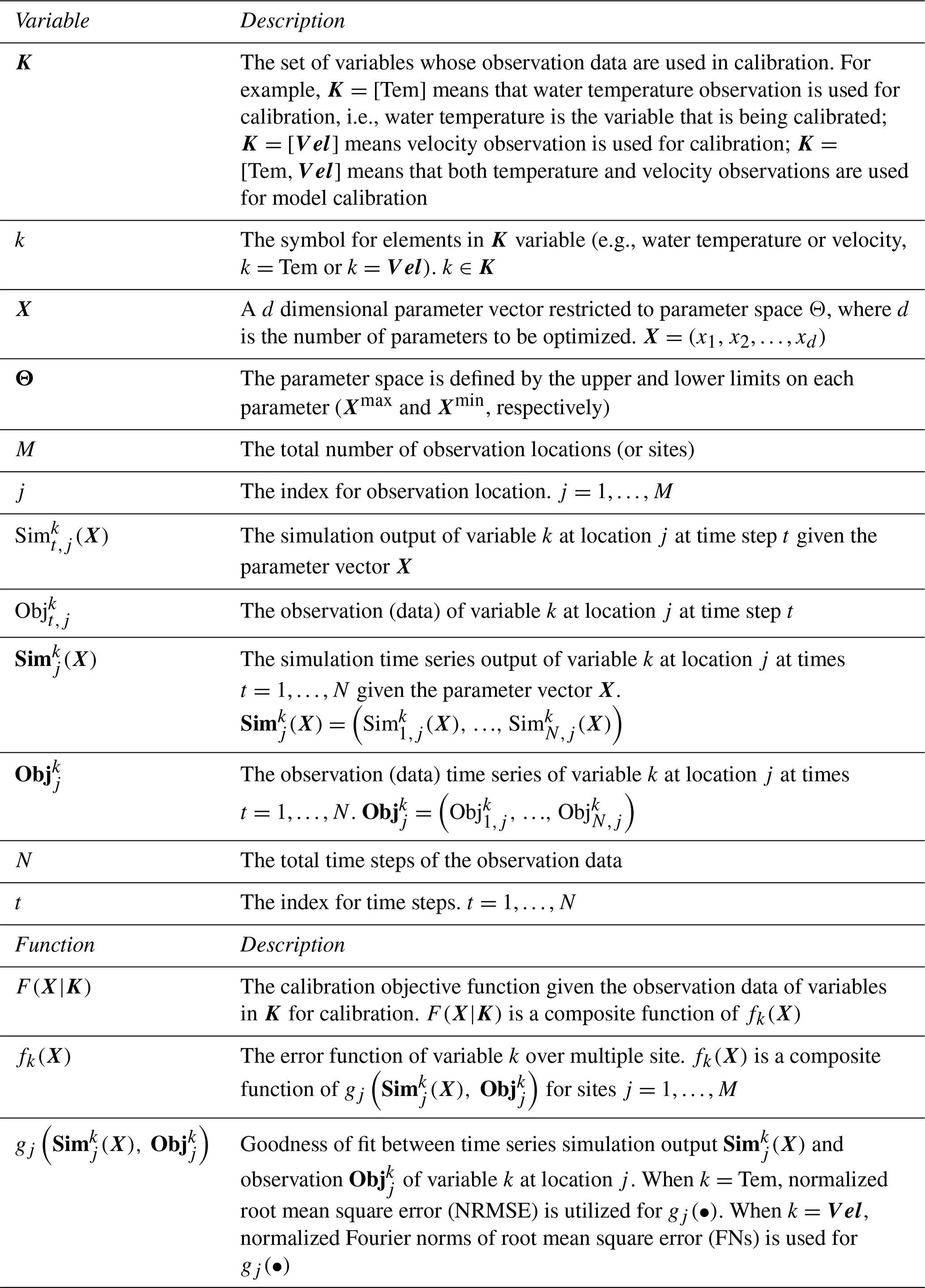
The calibration problems investigated in this study are multisite (i.e., observations are available from multiple locations), multivariable (e.g., temperature and velocity for hydrodynamics) problems, and are defined mathematically as follows (the variable and function definition are given in Table 1):
Note that the notation zi in Eq. (2) is simply meant to imply the function on the left depends on the finite series of quantities inside the braces { }.
Table 1Notation and definitions of variables and functions in Eqs. (1) and (2).
The set of parameters X being calibrated in this study includes nine parameters (d=9). Details of these parameters are provided in Table 2 in Sect. 2.4. The two variables calibrated in this study are velocity and temperature, for which data exist for different spatial locations and time points.
We investigate different calibration formulations, where either one or both of these variables are calibrated. Consequently, K=[Tem] means that water temperature observation is used for calibration, i.e., water temperature is the variable that is being calibrated; K=[Vel] means velocity observation is used for calibration; means that both temperature and velocity observations are used for model calibration, i.e., both variables are being calibrated simultaneously. The objective function in each scenario is discussed in Sect. 2.5.
2.2 DYNO for model calibration with multiple variables
One major issue for model calibration with multiple variables is how to formulate the error of multiple variables with a single objective function. In practice, different variables (e.g., temperature and velocity) usually have different physical units and magnitudes of error. Their error functions cannot be summed up directly into a single objective function if we wish to give the error of each variable an equal weight in the overall objective function. The respective error functions have to be normalized. There are goodness-of-fit metrics that can normalize the error of different variables (e.g., normalized root mean square error (NRMSE) and Kling–Gupta efficiency (KGE, Gupta et al., 2009)). However, it is still possible that the highest attainable value (or distribution) of NRMSE (or KGE) across the parameter space for one variable maybe be much higher than the highest attainable value (or distribution) of NRMSE (or KGE) of another variable. Hence, how to balance such differences among multiple variables is still important even when the normalized goodness-of-fit metrics are used.
We propose a new general objective function, DYNO, for the multivariable calibration problem. Let ψ be the set of evaluations found so far by the optimization, DYNO (as shown in Eq. 3) normalizes the error of each variable fk(X) with its upper and lower bound, and , of all evaluations in ψ. Since true values of bounds are not known, and are dynamically updated during the optimization search after each iteration. The mathematical formulation of the multivariable calibration problem, with DYNO, is as follows:
where and are the maximum and minimum values, respectively, of fk(X) for all evaluations in ψ. and have to be updated dynamically in each iteration during optimization. A detailed description of the implementation of Eq. (3) in the algorithm (i.e., PODS) tested in this study is given in Sect. 2.6.
2.3 Study site and data
We use a 3D model of a tropical reservoir as an example to test the efficiency of DYNO for multivariable calibration problems and to study the impact of using temperature and/or velocity data for model calibration. The horizontal boundary of the studied reservoir is given in Fig. 1a and b. The reservoir has over 250 ha of water surface with a maximum depth of about 22 m. One online water quality profiler station (STN. A1) was installed in the middle of the reservoir. The water temperature data at the station are available at various depths. The model is built for the simulation of the year 2013. One-year measured temperature data were used for model calibration in a previous study (Xia et al., 2021). We use this calibrated model to create synthetic observation data since the real velocity measurements are not available. We first assume a set of “true” model parameters XR. The value of XR is based on manual calibration by experts and is listed in Table 2. The spatial and temporal observation data for the hypothetical lake are synthetically generated based on the “true” model parameters XR. The synthetic observation data for the hypothetical temperate lake are generated by running the simulation model for 1 year with the vector of model parameters XR. The simulation output is then saved hourly in N time steps for multiple variables, i.e., temperature and velocity ( at M locations (specified in Fig. 1). In our study case, N=8761 and M=12 with different depths of five hypothetical sensor stations (STN. A1 and STN. B1–4 as shown in Fig. 1a and b).
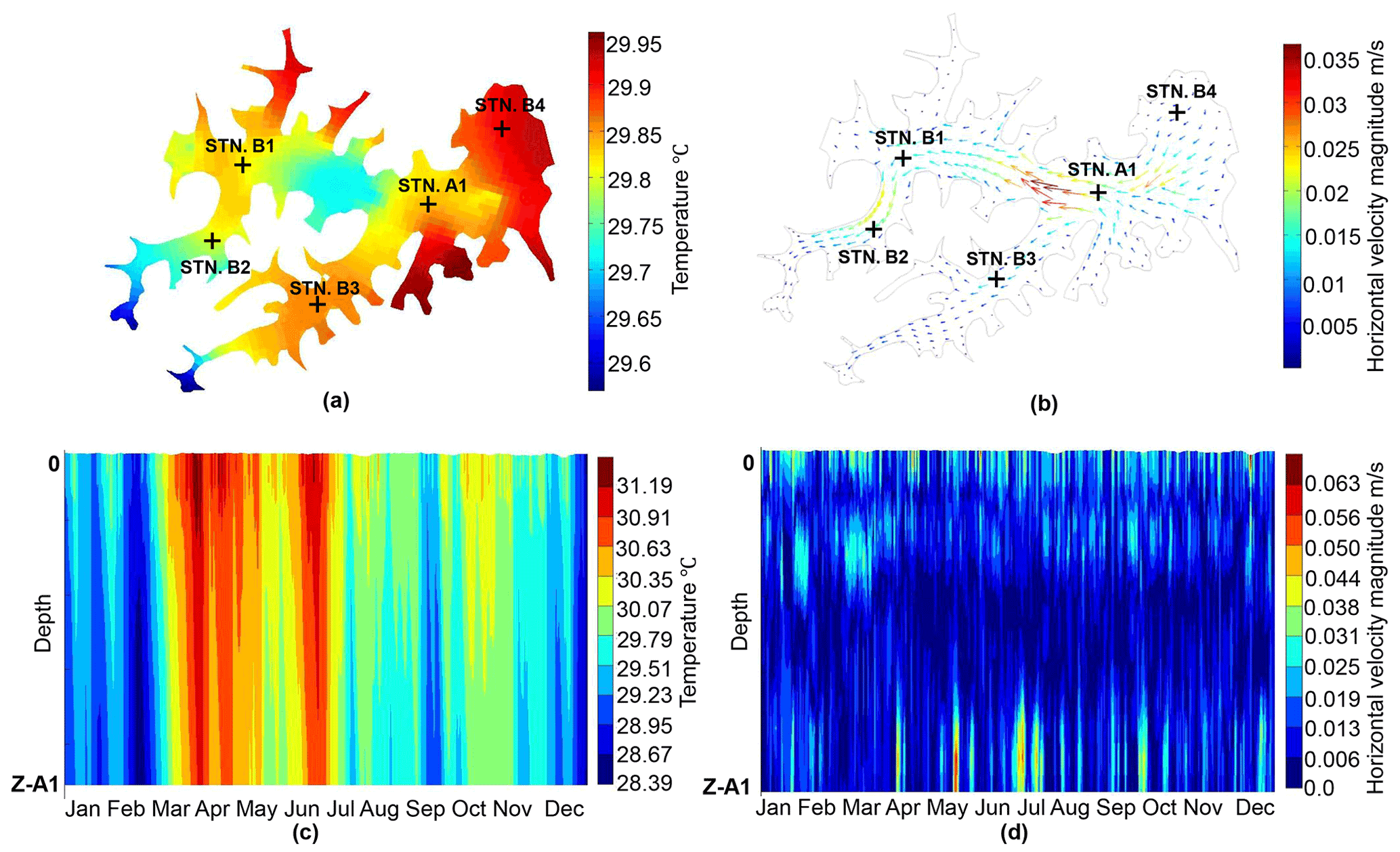
Figure 1Hydrodynamic model simulation results (with “true” model parameters) for the year 2013. (a) Simulated temperature spatial distribution with sampling locations. (b) Simulated velocity spatial distribution with sampling locations. (c) Time–depth plot of simulated temperature at STN. A1. (d) Time–depth plot of velocity magnitude at STN. A1. Z-A1 is the maximum water depth at station A1.
Table 2Model parameters used in calibration. XR denotes the true solution used to generate synthetical temperature and velocity observations at multiple sites.

a Deltares (2014); b Chanudet et al. (2012); c Wahl and Peeters (2014); d Råman Vinnå et al. (2017); d Soulignac et al. (2017); e Pijcke (2014).
The saved hourly simulated output time series is denoted as , which as defined (in Table 1) contains information for each time step, t=1, … N. Thus Γ is used as observation data for model calibration, i.e., in Eq. (1). In the test of optimization for calibration, the true values of the parameter vector XR are not provided to the optimization. The optimization will, instead, search for the best set of X that will minimize the objective function F(X|K), where K=[Tem], [Vel], or [Tem,Vel]. Hence the goal of automatic calibration via optimization is to obtain an optimum calibration X* that results in simulation model output, , j=1, …, M, (see Eqs. 1 and 2) that is close to the synthetic observation time series data in Γ.
The temperature and velocity simulation results in the year 2013 based on the “true” model parameters (shown in Table 2) show temporal and spatial variation, as presented in Fig. 1a–d. Figure 1a and b show the temperature and horizontal velocity distribution at the surface layer. Figure 1c and d show the distribution of temperature and velocity magnitude at STN. A1. There is obvious temperature stratification in the vertical direction (as shown in Fig. 1c). We have five sampling locations across the reservoir. The observation data at these five locations are used to calibrate the model parameters.
2.4 Hydrodynamic model and calibration parameters
The description of the hydrodynamic model is given in Xia et al., (2021). The hydrodynamic model is built with Delft3D-FLOW (Deltares, 2014). The Delft3D-Flow hydrodynamic model used was set up by the water utilities' employees and consultants, including the domain construction, input data preparation, and model configuration. The grid coordinate system is based on Cartesian coordinates (Z grid), which have horizontal coordinate lines that are almost parallel with density interfaces to reduce the artificial mixing of scalar properties such as temperature. The number of grid points in the x direction is 65, the number of grid points in the y direction is 67, and the number of layers in vertical is 19. A single 1-year simulation takes about 5 h to run in serial order on a Windows desktop with CPU Intel Core i7-4790.
There are nine tunable model parameters (listed in Table 2) in the model. The first five parameters in Table 2 are related to the turbulence calculation. The k-ε closure model (Uittenbogaard et al., 1992) was chosen as the turbulence closure model to calculate the viscosity and diffusivity of the water. The calculation of the viscosity and diffusivity involves five parameters: (1) background viscosity in horizontal direction , (2) vertical direction , (3) the background eddy diffusivity in horizontal direction , (4) vertical direction , and (5) the Ozmidov length Loz. These parameters affect both the velocity and the temperature. The vertical exchange of horizontal momentum and mass is affected by vertical eddy viscosity and eddy diffusivity coefficients (Elhakeem et al., 2015). The horizontal velocities are affected by the horizontal eddy viscosity and diffusivity coefficients (Chanudet et al., 2012). Chanudet et al. (2012) highlighted that the most impactful parameter for temperature is the background vertical eddy viscosity and the Ozmidov length Loz also has a significant effect on the thermal stratification by affecting the vertical temperature mixing.
The next three parameters in Table 2 are related to the simulation of surface heat flux. In the heat flux model, the evaporative heat flux and heat convection by forced convection are parameterized by the Dalton number ce and Stanton number cH, respectively, which are also in the list of calibration parameters. The Secchi depth HSecchi (also included in Table 2) is another parameter required by the ocean heat flux model. Secchi depth is related to the transmission of radiation in deeper water and thus affects the vertical distribution of heat in the water column (Chanudet et al., 2012). Heat fluxes through the reservoir bottom were not simulated in the current model. The last parameter is the Manning coefficient, which affects the roughness of the bottom of the lake and has a direct impact on velocity.
All of these nine parameters affect (either directly or indirectly) the thermal and current activity in the water body. These are also the parameters included in the routine model calibration by local experts and, thus, are included in the calibration process in our study. The calibration range for these parameters (given in Table 2) is suggested by Singapore water utilities employees and consultants. Some of these parameters might be spatiotemporally variant (such as Secchi depth, Ozmidov length scale, Dalton number, and Stanton number). Considering these parameters as time- or space-varying parameters will substantially increase the number of decision variables in optimization. Considering that the reservoir in our study is relatively small and is located in a tropical region where there is no significant seasonal variation, we consider these parameters to be constant across space and time.
2.5 Calibration problem formulation
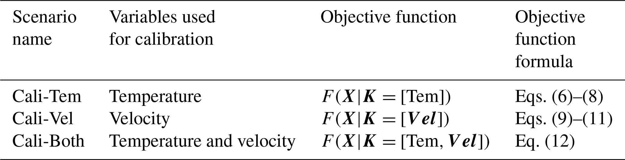
Three scenarios are considered to investigate the impact of model calibration against temperature and/or velocity observations (as discussed in Sect. 2.1). The first two scenarios calibrate to only one variable, and the last scenario calibrates both variables simultaneously. This section gives the detailed calibration formulations of these three scenarios.
2.5.1 Model calibration with one variable
The objective functions for Cali-Tem and Cali-Vel scenarios are summarized in Eqs. (6)–(11), where only observations of one variable are included in the calibration.
where, and denote the NRMSE of temperature (described in Eq. 8), and normalized FNs of velocity vectors (described in Eq. 11) at locations j. and denote the simulated velocity given a parameter vector X and observed velocity, respectively, at time step t and location j. and are 3D vectors. ∥-∥2 in Eq. (11) is the Euclidean norm used to quantify the size of a vector.
The temperature and velocity data are taken at different depths of multiple stations, and their magnitude at different locations might be different due to spatial variation. Hence, the fitness at each location should be normalized before being summed into the objective function. For water temperature, NRMSE (as described in Eq. 8) is used to quantify and normalize the error between the simulated and observed data. For velocity, normalized FNs (as described in Eq. 11) are used to measure the error between the model-simulated and observed data (corresponding simulated and observed velocity data points are 3D vectors). The calculation of the FN follows the description in Beletsky et al. (2006), Huang et al. (2010), Paturi et al. (2014), and Råman Vinnå et al. (2017).
Table 3Summary of objective function formulations for different calibration scenarios.
2.5.2 DYNO for model calibration with multiple variables
In the Cali-Both scenario, both temperature and velocity are calibrated simultaneously, which can be treated as a bi-objective function problem. The objective function in the Cali-Both scenario (as shown in Eq. 12) applies the DYNO proposed in Eq. (3). The error functions for water temperature, i.e., fTem(X), and velocity, i.e., fVel(X), are the objective functions of the Cali-Tem scenario (Eq. 7) and the Cali-Vel scenario (Eq. 10), respectively. The temperature and velocity errors are dynamically normalized with their upper and lower bounds during the search of the optimization algorithm before being summed into a single objective function. The mathematical formulation of the objective function in the Cali-Both Scenario (based on Eq. 3) is as follows:
where the maximum and minimum of fTem(X) and fVel(X) are updated after each optimization iteration (since new parameter sets are sampled in each optimization iteration). As the number of iterations increases, the denominators in Eq. (12) also increase since the optimization method finds better minimum objective function values. Hence the individual objective function components (for each variable) scale dynamically to maintain an approximately equal weight of the terms related to temperature and velocity.
As defined in Eqs. (6)–(12), three calibration formulations are investigated in this study. Table 3 gives a summary of these calibration formulations.
2.6 Implementation of DYNO with PODS
In this section, we describe the implementation details for incorporating DYNO into a new efficient parallel surrogate optimization algorithm, PODS (described in Fig. 2). PODS (Xia et al., 2021) is a parallel version of the serial DYCORS (DYnamic COordinate search using Response Surface models) algorithm introduced by Regis and Shoemaker (2013). DYCORS is an iterative surrogate method (such methods are sometimes also called “response surface optimization methods”, where cheap surrogates of the expensive objective are built to improve optimization efficiency), designed for optimization of computationally expensive black-box functions within a limited number of evaluations. DYCORS uses RBF (radial basis function) as surrogates to efficiently explore the parameter space and propose promising new solutions for expensive evaluation in each algorithm iteration. The RBF-guided search methodology of DYCORS is designed for high-dimensional black-box optimization within a limited number of evaluations of computationally expensive real objective functions. PODS, like DYCORS, is designed for black-box optimization problems that are high-dimensional and computationally expensive and have multiple local minima. Xia et al. (2021) show that PODS is considerably more efficient than other parallel global optimization methods in obtaining good solutions with fewer objective function evaluations, which is very important for expensive objective functions like hydrodynamics models. PODS parallelized the serial DYCORS algorithm by following the master–worker framework (as shown in Fig. 2). This parallelization strategy of the algorithm enables simultaneous function evaluations on multiple processors (cores) in batch mode, which reduces the wall-clock time of the optimization process. This can greatly speed up the calibration of computationally expensive models and make the calibration of some extremely expensive models computationally tractable.
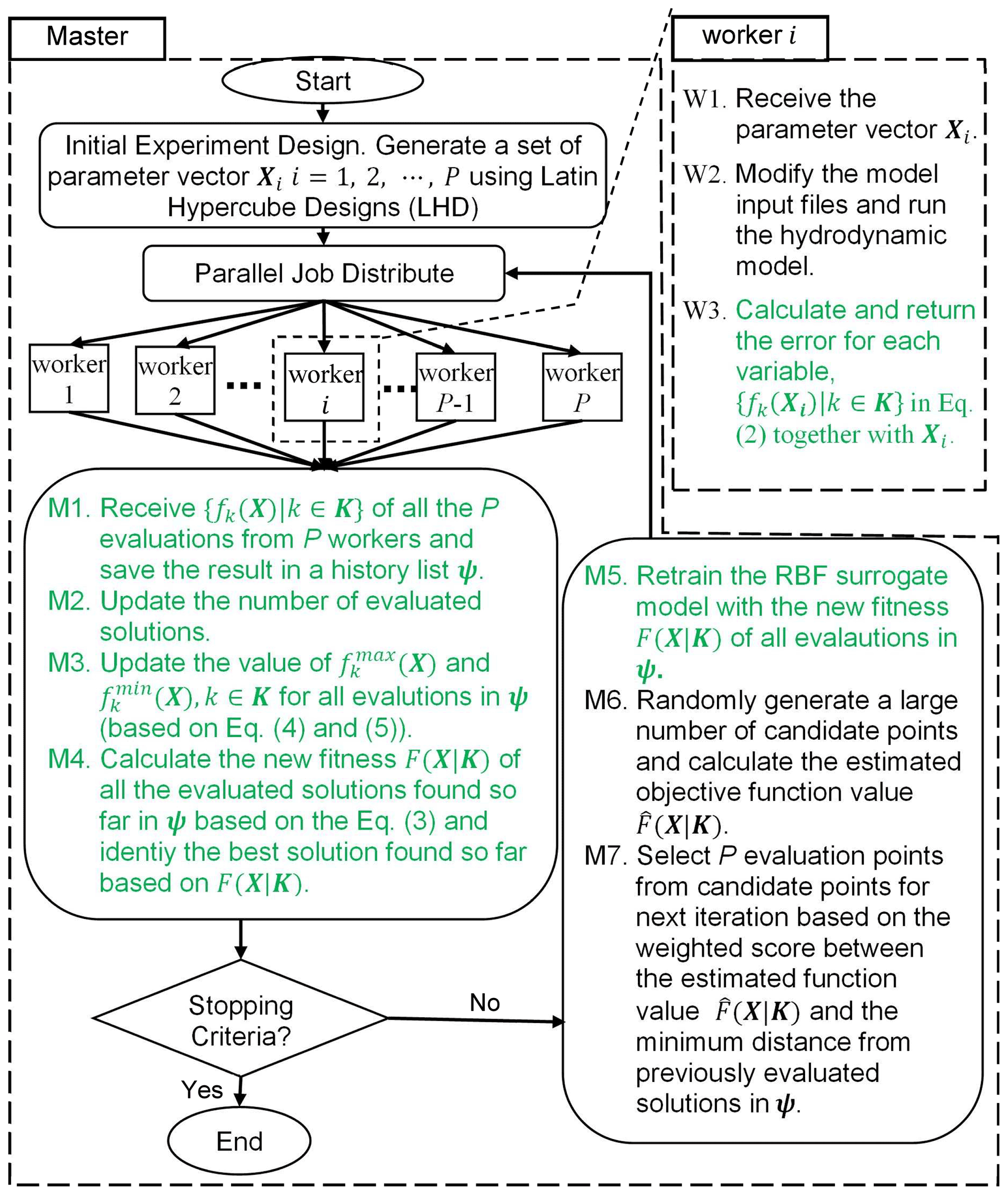
Figure 2Diagram of the implementation of DYNO with the parallel algorithm PODS. P is the number of processors available. The green texts (i.e., steps W3, M1–5) are changes made on PODS to incorporate DYNO. The rest of the text follows the original PODS method.
The PODS algorithm begins the optimization from an initial experiment design where a random initial set of evaluation points are generated with the Latin hypercube design (LHD). These evaluation points are distributed randomly to P workers for simulation evaluations. Each worker will calculate the error or objective function of each variable {fk(Xi)|k∈K} based on Eq. (2) and return them to the master. This step (W3 in Fig. 2) for DYNO-based PODS is different from the original PODS. In the original PODS, only the final objective function value (instead of the error of each variable) is returned to the master.
After the master collects the results of all the Pevaluations, it will add these new results into the history list ψ that saves all evaluation results found in previous iterations. The history list of ψ is not in the original PODS and it is necessary for the calculation of the DYNO objective function (F(X|K), X) (as shown in Eq. 3). For instance, the maximum and minimum value of the error of each variable and , respectively, are dynamically changing with the increase of the history list ψ. The objective function value F(X|K) for all evaluations found in current and previous iterations needs to be recalculated because of the update of and . And the best solution found so far is identified based on the newly calculated F(X|K). When only one variable (e.g., temperature or velocity) is considered in the objective function, the best solution is the evaluation with the lowest error between the simulation output and observations of the variable considered. In cases where multiple variables are considered in calibration, the best solution should be the evaluation with the smallest value of F(X|K) after considering the error of multiple variables (as shown in Eq. 3). Because the objective function value for all evaluations in ψ changed after each iteration, the RBF is also rebuilt with these new objective function values of all evaluated solutions (F(X|K), X). The rebuilt RBF surrogate is used for the generation of the evaluation points for the next iteration.
PODS with DYNO implementation uses the RBF surrogate in the same way as the original PODS does. PODS first generates a large number of candidate points around the best solution found so far (refer to Sect. 2.2 in Xia et al., 2021). The algorithm then selects P evaluation points from these candidate points on the basis of their estimated objective function based on the RBF surrogate and the minimum distance from all previous evaluation solutions in ψ. A lower estimated objective function is better since it is more likely to lead to solutions with lower objective function value. Moreover, candidate points that are far from previous solutions are also preferred since they help the algorithm to explore regions of the solution domain that were not explored in previous iterations. These unexplored regions could possibly be regions where better solutions are located. The consideration of estimated objective function and distance information are both considered when selecting the candidate points through a weighted score based on these two aspects. For detailed information on the implementation of evaluation point selection criteria, one can refer to Sect. 2.3 in Xia et al. (2021). The selected P evaluation points are then distributed to P workers for evaluations, and the iteration loop continues until the stopping criteria are met (e.g., the computing budget is finished).
In summary, the implementation of DYNO affects the selection of the best solution found so far and also the surrogate model (these steps are W3 and M1–5, as highlighted in green in Fig. 2). We should stress that the fitting of the surrogate model is computationally inexpensive compared with the runtime of the expensive objective function. Hence it does not affect the overall algorithm runtime.
2.7 Experiment setup
All computational experiments in this study are implemented on a single node on the National Supercomputer Center (NSCC) of Singapore, which is a Linux-based platform with dual Intel Xeon E5-2690 v3 processors, with each node having 24 cores. Hence, we set the number of processors P to be 24. Due to the stochastic nature of the optimization algorithm (i.e., PODS) used in this study, multiple optimization runs are executed for each calibration experiment in Table 3. Considering that the calibrated hydrodynamic model in this study is extremely expensive, we perform three optimization trials for each calibration experiment (see Table 3 for a list of experiments). Furthermore, to remove any initial sampling bias, each concurrent optimization trial for the three calibration experiments is initialized with the same Latin hypercube experimental design (thus the calibration in each scenario starts from the same initial solutions). We also investigated the performance of different forms of DYNO on the Cali-Both scenario.
We set the same evaluation budget (i.e., the maximum number of hydrodynamic model runs) for each trial and calibration scenario (i.e., Cali-Tem, Cali-Vel, and Cali-Both). The maximum number of hydrodynamic model runs in each trial is 192, which is 8 iterations with 24 evaluations in each iteration. Our result indicates that eight iterations is a sufficient calibration budget, as the calibration progress plot in Fig. S1 in the Supplement shows that the optimization experiments almost converged in the last few iterations.
The computational time of one simulation is approximately 5 h on a Windows desktop with a CPU Intel Core i7-4790 processing unit. However, when running 24 simulations simultaneously on the multicore platform, the computational time gets longer because of the limited cache memory resources (as discussed in Xia and Shoemaker, 2022a). Cache memory is a small amount of much faster memory than main memory. The wall-clock time for one iteration with 24 cores simultaneously running is about 12 h if using the default process scheduling of the nonuniform memory access (NUMA) multicore system. We used the mixed affinity scheduling proposed by Xia and Shoemaker (2022a), and the wall-clock time is reduced to about 8 h per iteration. The mixed affinity scheduling changed the default affinity setting by setting a hard affinity on the simulation of each PDE model (i.e., fixing the process of each PDE simulation to one core). This approach proved to be efficient for memory usage and reduced the simulation time. More details about the mixed affinity scheduling and the NUMA system can be found in the study by Xia and Shoemaker (2022a). Hence, the wall-clock time of each trial takes about 64 h (8 iteration × 8 h/iteration).
3.1 Comparison of calibrating to temperature and/or velocity
3.1.1 Final solutions in goodness-of-fit metrics
We first compare the three calibration formulations in terms of goodness-of-fit metrics for both temperature and velocity. Table 4 summarizes this comparison for the three formulations, i.e., (i) Cali-Tem, (ii) Cali-Vel, and (iii) Cali-Both (see definition in Table 3), with PODS used as the optimization algorithm and with a budget of 192 simulations.
Table 4Summary table of the solution obtained by PODS for each scenario (Cali-Both, Cali-Vel, and Cali-Tem). fTem(X*|K) and fVel(X*|K) are the temperature error fTem(X*) and velocity error fVel(X*) (calculated in Eq. (7) and Eq. (10), respectively, with the optimal solution X* obtained in each trial). The mean and standard deviation of fTem(X*|K) and fVel(X*|K) among three trials are reported. The variable error is bold in each scenario when the observation of the variable is included in the calibration in each scenario. (Some terms defined in Table 1).
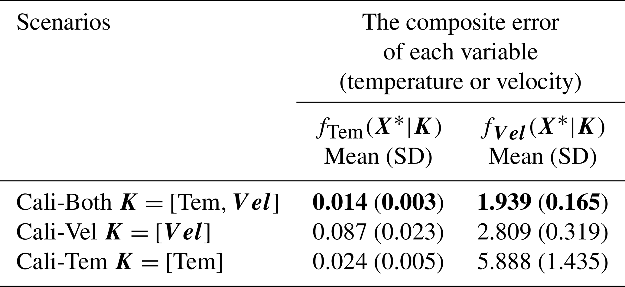
The mean as well as the standard deviation of both temperature error fTem(X*|K) (calculated as Eq. 7) and velocity error fVel(X*|K) (calculated as in Eq. 10) over three trials are reported in Table 4, for all three calibration scenarios. X* in Table 4 denotes the optimal calibration solution obtained by PODS in each trial for a given scenario (defined by the set of variables K). The solution with the lowest variable error (fTem(X*) or fVel(X*)) is highlighted in bold in Table 4. Table 4 reports the variable errors of both temperature and velocity for all formulations to understand the impact of excluding or including a variable in the calibration formulation. Please note that the temperature error, fTem(X|K=[Tem]), reported in Table 4, is exactly the calibration objective function in the Cali-Tem scenario (F(X|K=[Tem]) as shown in Eq. 7). Similarly, the velocity error fVel(X|K=[Tem]) is exactly the calibration objective function in the Cali-Vel scenario (i.e., F(X|K=[Vel]) as shown in Eq. (10). We use the word “variable error” instead of “objective function value” when referring to the values in Table 4 in subsequent discussions since we are in part looking at the impact of using data from one variable to predict another variable for which we do not have data. It is also worth mentioning that the value in Table 4 is a sum of temperature or velocity error at multiple (in total 12) locations. Hence the error at each location is smaller than the value in the table.
Table 4 shows that the solution obtained when calibrating to temperature observation only (Cali-Tem) has smaller temperature errors but larger velocity errors than that if calibrating to velocity observation data only (Cali-Vel). However, it is surprising that when calibrating to both temperature and velocity (Cali-Both), the solution obtained by PODS has the lowest temperature and lowest velocity error compared with calibrating to either temperature observation or velocity observation only. This might be because calibrating to temperature will help to improve the fit of velocity and vice versa. This makes sense because water temperature and velocity are two related variables in hydrodynamic modeling, and they affect each other. Velocity is the fundamental variable of hydrodynamics with directional information not provided by temperature; temperature (via the heat flux model) may also affect the velocity field since it affects water density. Our analyses here are based on physical models, which are built based on physics laws and knowledge humans have acquired over hundreds of years. Our findings here are in line with the study by Baracchini et al. (2020), who also suggested having both temperature and velocity for a complete system calibration.
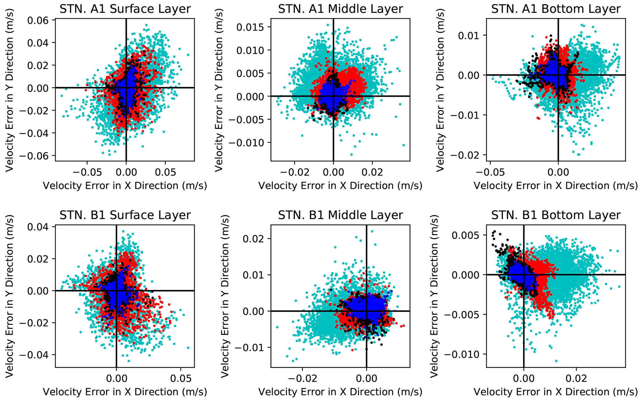
Figure 3Scatter plot of velocity error ΔVel in horizontal (X and Y direction) between simulated velocity and observed velocity at location j. Each dot denotes the velocity error ΔVel of location j at one time step. j = surface layer of STN. A1 for upper panel and j = STN. B1 for lower panel. X* is the optimal solution found by PODS in each scenario: Cali-Tem (red dots), Cali-Vel (black dots), and Cali-Both (blue dots) as listed in Table S1. The “true” solution is on or near the intersection of the two perpendicular black lines. An initial uncalibrated solution (cyan dots) is plotted for reference.
3.1.2 Visual comparison of calibration errors
The above analysis is based on the average variable error statistics only (i.e., fTem(X*|K) and fVel(X*|K)), of the best results obtained from PODS (over multiple trials) for all calibration scenarios. In order to further analyze the difference between calibration formulations (in terms of their effectiveness in calibrating both temperature and velocity), we visually compare the best calibration solutions (X*) obtained by PODS for each scenario, i.e., Cali-Tem, Cali-Vel, and Cali-Both. We select one representative optimal solution (X*) from three trials in each scenario for this comparison. An initial uncalibrated solution is included in the comparison. The parameter value of the uncalibrated solution (in Table S1 in the Supplement) uses the mean of the calibration range in Table 2.
The objective function value in terms of temperature and velocity composite error (over multiple locations) (fTem(X) and (fVel(X), as formulated in Eqs. 7 and 10, respectively) and the corresponding parameter configuration (X*) of the selected solution (among three trials) are plotted in Fig. 5 and reported in Table S1. In general, the solution in the Cali-Both scenario is closer to the true solution than solutions in the other two scenarios in terms of parameter values. Calibrated values proposed by the Cali-Both scenario are closest (relative to other scenarios) to the true values for four parameters (i.e., , , HSecchi, cH). Moreover, besides the Manning coefficients, the calibrated values proposed by the Cali-Both scenario are not the worst (relative to the other two scenarios) for any other parameter. By contrast, calibrated values proposed by the Cali-Tem scenario are the worst (i.e., the parameter values are farthest from the true solution, relative to other scenarios) for five parameters (i.e., , , , , ce) and calibrated parameter values for the Cali-Vel scenarios are the worst for Loz, HSecchi, cH. This indicates that calibrating to both temperature and velocity can help to prevent the value of the nine calibration parameters from being very far from the corresponding value for the true solution.
The horizontal velocity error ΔVel (2D) between simulated velocity and observed velocity (in the horizontal plane) is plotted as scatter plots of time series in Fig. 3 (for all calibration scenarios). The temperature error ΔTem between simulation temperature and observed temperature is plotted as a time series (for each calibration scenario) in Fig. 4.

Figure 4Time series plots of temperature error ΔT between simulated water temperature and and observed water temperature () at location j where j = surface layer of STN4 for left panel and j = STN1 for the right panel. X* is the optimal solution found by P-DYCORS in each scenario: Cali-Tem (red lines), Cali-Vel (black lines), and Cali-Both (blue lines) as listed in Table S1. An initial uncalibrated solution (cyan lines) is plotted for reference.
The error plots for the two sampling locations at multiple depths (i.e., surface layers of station STN. A1 and STN. B1 as shown in Fig. 1)) are visualized in Figs. 3 and 4 (for 1 year). Since the velocity error ΔVel at a particular time and location is a vector (and not a scalar like temperature) and velocity error in three dimensions (for a time series) is hard to represent visually, Fig. 3 only plots the velocity error (for 1 year) ΔVel in the horizontal plane (i.e., X and Y directions only). Moreover, each dot represents the error at one point in time during the study period.
Figure 3 plots the difference between the simulated velocity (for the optimized parameter values obtained from Cali-Tem (red scatter points), Cali-Vel (black scatter points), and Cali-Both (blue scatter points) scenarios) and observed velocity. Ideally, the error for each scatter point should be zero, i.e., at the intersection of the two lines. Figure 3 illustrates that calibrating to temperature data only (red scatter plot) results in a larger velocity error ΔVel, relative to velocity error when calibrating to velocity data only (Cali-Vel scenario, i.e., black scatter plot) or to both velocity and temperature data (Cali-Both scenario, i.e., blue scatter plot). Figure 3 also shows that solutions of all the three scenarios improved the temperature fit compared with the initial solution, which demonstrates the effectiveness of the optimization calibration.
Figure 4 shows the temperature error of solutions from three different calibration scenarios: Cali-Tem (red time series), Cali-Vel (black time series), and Cali-Both scenarios (blue time series). The errors between simulated and observed water temperature at the surface, middle, and bottom layers of two stations (STN. A1 and STN. B1) are plotted. In general, the temperature error of the solution in the Cali-Both scenario is generally close to 0 ∘C for all the layers and stations shown. The solution in the Cali-Tem scenario also achieved temperature errors close to 0 ∘C in the middle and bottom layer at STN. A1, but it has larger temperature errors than the solution in the Cali-Both at the surface layer of STN. A1 and all layers of STN. B1. The solution in the Cali-Vel scenario generally overestimated the water temperature in all locations (i.e., all the surface, middle, and bottom layers at both stations). The temperature error of the solution in the Cali-Vel scenario is much larger than that of the solution in Cali-Tem and Cali-Both scenarios in the middle and bottom layers of both stations. The temperature error at most times, for the Cali-Vel scenario, is greater than 0.1 ∘C. This might be because both the Stanton and Dalton numbers are underestimated in the Cali-Vel scenario when compared with the true solution (XR) (as shown in Fig. 5). The Dalton number Ce affects the evaporative heat flux modeling and the Stanton number CH influences the convective heat flux modeling in the Delft3D-FLOW model (Deltares, 2014). For the solution in Cali-Vel, a smaller Stanton number CH (shown in Fig. 5) might lead to underestimated convective heat flux, which will lead to the overestimation of the water temperature. In summary, calibrating to temperature and velocity (i.e., Cali-Both) gives the best solution in terms of temperature error compared with calibrating to temperature or velocity only (i.e., Cali-Tem or Cali-Vel). Calibrating to velocity only (Cali-Vel) gives the worst result in terms of temperature fit. Simulation of vertical temperature, vertical velocity, vertical eddy diffusivity, and vertical eddy viscosity (Figs. S2–S5) also shows that the solution in the Cali-Both scenario is much better than solutions in the Cali-Tem and Cali-Vel scenarios. For example, the solution in the Cali-Both scenario can almost capture the vertical time-varying temperature profiles of the true solution. By contrast, calibrating to one variable did not fully capture the vertical time-varying temperature profiles (e.g., April–May for the Cali-Tem scenario; March–May and August–September for the Cali-Both scenario in Fig. S2). The solution in the Cali-Both scenario also gives much smaller vertical velocity, eddy diffusivity, and eddy viscosity error than solutions in the other two scenarios (in Figs. S3–S5). The results indicate that using both temperature and velocity data in model calibration also helps to improve the complex time-varying vertical mixing behavior.

Figure 5Parallel axis plot for the parameter value and the composite error of temperature and velocity of calibration solutions under different scenarios (Cali-Tem, Cali-Vel, and Cali-Both). True solution defined in Table 2 is given for reference. Smaller variable errors (fTem(X), see Eq. 5 and fVel(X), see Eq. 8) are better, and the variable errors of the true solution (XR) are zero (for both fTem(X) and fVel(X)). The parameter symbols are defined in Table 2.
3.2 Optimization search dynamics under different calibration scenarios
We further analyze the calibration progress of PODS for Cali-Tem, Cali-Vel and Cali-Both, to understand the calibration convergence speeds of the three formulations. The purpose of the calibration progress analysis is to visualize the improvement in calibration quality of both temperature and velocity variables from the LHD, for all three formulations. As discussed in the experiment setup section, we conducted eight iterations of the optimization search. This is a reasonable number of iterations for our case, given that (1) the problem is computationally expensive (one experiment takes about 64 h to run and there are nine experiments) and (2) the calibration progress plot in iterations (Fig. S1) indicates that the optimization search almost converged in eight iterations.
Figure 6 plots the calibration progress of the three formulations (i.e., Cali-Tem, Cali-Vel, and Cali-Both) using PODS. Each subplot in Fig. 6 corresponds to the different concurrent optimization trials (i.e., trials of the stochastic optimization method using the same initial points from LHD) for each formulation. The best solutions are near the origin of each graph. Moreover, Fig. 6 plots the progress (quantified by visualizing both temperature and velocity errors) of the best solution found (measured in terms of the objective function value in each calibration scenario) during the search. Figure 6 indicates that when calibrating to temperature or velocity only, the optimization search cannot guarantee the improvement of the fit of another variable. For example, in Fig. 6a, when calibrating to velocity only, the temperature error of the best solution found at the end of the optimization search stage is worse than the temperature error of the best solution found after the initial LHD, even though there is improvement in terms of velocity fit. Similarly, when calibrating to temperature only, the improvement in velocity fit is also not significant (for instance, in Fig. 6a). When calibrating to the fit of both temperature and velocity using the DYNO formulation, the fit of both temperature and velocity improves in all trials, and the improvement remains balanced during the optimization search. Figure 6 also indicates that the final solution found in Cali-Both scenarios dominates the best solution found by PODS in Cali-Tem and Cali-Vel in terms of both temperature and velocity fit.

Figure 6Calibration progress plot of the best solution found (in terms of objective function value) during optimization search by PODS when calibrating to temperature only (Cali-Tem), calibrating to velocity only (Cali-Vel), and calibrating to both temperature and velocity (Cali-Both). Three random trials (i.e., T1, T2, and T3) are plotted in (a)–(c). Lower velocity and temperature error are better. The yellow markers are evaluation points in the initial experiment design using LHD. Besides solutions in LHD, only the best solution in each of the optimization iterations is plotted (i.e., markers joined by lines). The line links the best previous solution in one iteration to the best solution in next iteration. The arrow indicates the direction from the previous solution to the next solution.
Figure 6 also shows that when calibrating to one variable, the optimization search is easily convergent (i.e., the best solution does not continue improving after a few iterations even in terms of the fit of the variable considered in calibration). For example, in Fig. 6a, when calibrating to temperature only, the best solution in terms of temperature error does not improve much (in the last few iterations). The reason might be that when the velocity error is large, it is less likely that the temperature fit would be improved further. By contrast, when calibrating to both temperature and velocity, the optimization search continues improving in both the temperature and velocity fit. Hence only considering one variable in the calibration, it is difficult to get a solution that has small (or close to zero) errors of the variable considered. We should also stress that even though the optimization gets a solution that has zero error in one variable, it does not mean that the error of another variable would be zero. The reason is that only the observation in part of the simulation space is used for calibration (not the observation data at each grid and each time step of the simulation space that are used to calculate the temperature error). Thus, the temperature error may be zero at these observation locations, while the temperature error is not zero at other locations where observation is not used in the calibration. In this case, getting a temperature error of zero for the observation locations cannot guarantee the velocity error is zero.
It is also important to understand the “frequency” or likelihood with which PODS can find good temperature and velocity calibrations via the three different formulations proposed in this study. Hence, we also do a comparative frequency analysis of the errors (for velocity or temperature) of all evaluated points (, …, 3×Nmax) from all trials (three trials) of PODS when using different calibration formulations (see Table 3). The purpose of this frequency analysis is to understand the likelihood with which the three different formulations can obtain good velocity and temperature calibrations. The frequency analysis results are presented in Fig. 7 via visualizations of empirical histograms of both velocity error and temperature error (from all solutions of three trials of PODS) for each calibration scenario.
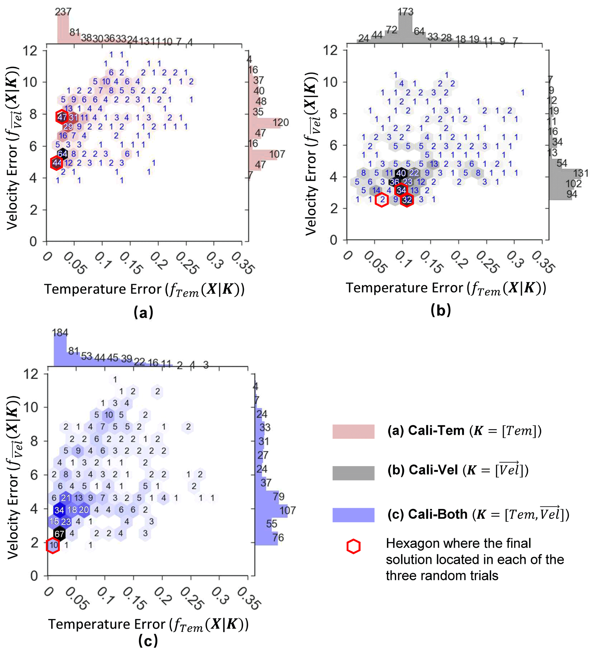
Figure 7Distribution plot of all the evaluated points found by PODS (over three trials) in terms of temperature composite error fTem(X|K) and velocity composite error fVel(X|K) in each scenario: Cali-Tem (K=[Tem]), Cali-Vel (K=[Vel]), and Cali-Both (). The number inside each hexagon represents the number of evaluated points located in that hexagon (e.g., with the combination temperature and velocity error associated with the corresponding values on the axes.) A darker color in the hexagon means a larger number of evaluated points is located in that hexagon. The bar plot along the upper x axis (fTem(X|K)) shows the distribution of the evaluation points in terms of temperature error only. The bar plot along the y axis (fVel(X|K)) is the distribution of the evaluation points in terms of velocity error only. The number above the bar shows how many evaluated points are located in that bin. Smaller error (fTem(X|K) or fVel(X|K)) is better. The true solution (fTem(XR|K), fVel(XR|K)) is the origin of each subplot.
Figure 7 plots the error distribution of all the evaluated points over three trials (576 evaluations) for each scenario: Cali-Tem (K=[Tem]), Cali-Vel (K=[Vel]), and Cali-Both (). The different subplots in Fig. 7 provide a visualization of the velocity (vertical axis) and temperature (horizontal axis) error distribution via hexagonal bin (hexbin) plots (inside the square) and error histograms (outside the square) for each of the calibration scenarios. The number inside each hexbin denotes the number of evaluated points (for that combination of temperature error and velocity error) located in that hexbin. Furthermore, the hexbin with a larger number of evaluated points is highlighted with a darker shade. The temperature histogram columns (above the square) represent the sum of all the hexbins inside the square directly beneath the number in the column. For the velocity histogram (on the right side of the square), the column height depends on the sum of all the hexbins in the row to the left of the number.
The temperature and error velocity distribution visualizations of Fig. 7 clearly show that calibrating to both temperature and velocity data (see Fig. 7c, i.e., error distribution for the Cali-Both scenario) provides good temperature and velocity calibrations with a higher frequency. Figure 7c shows that it is highly likely that both temperature and velocity errors are lower (indicated by darker hexbins with temperature error fTem(X|K) less than 0.05 and velocity error fVel(X|K) less than 4). Consequently, Fig. 7c also illustrates that the newly proposed DYNO (see Eq. 3) works effectively, in this case, to calibrate multiple variables simultaneously.
Figure 7 also illustrates that it is better to calibrate the hypothetical hydrodynamic model to velocity data rather than temperature data (see Fig. 7a and b) (if data for both variables are not available). Figure 7a indicates that calibrating to temperature only (i.e., the Cali-Tem scenario) results in a greater likelihood that velocity error would be high (see the velocity error histogram in Fig. 7a). However, Fig. 7b illustrates that the errors in temperature when calibrating to velocity only (Cali-Vel) are likely to be relatively small in magnitude (see the temperature error histogram of Fig. 7b).
From the above discussion, we can conclude that calibrating to both temperature and velocity data with the newly proposed DYNO (implemented within the efficient surrogate algorithm PODS) is effective in obtaining a balanced calibration of both temperature and velocity variables. In real-world hydrodynamic lake applications, if available, both temperature and velocity data should be used for lake hydrodynamic model calibration. However, the very common practice of calibrating only to temperature data is shown to be unable to reproduce the flow dynamics well. This supports the extra effort and expense to collect velocity data that is expected to give a beneficial effect.
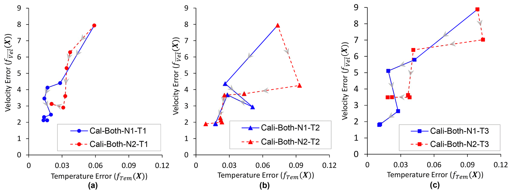
Figure 8Calibration progress plot in terms of the best solution found during optimization search when using DYNO-N1 and DYNO-N2 as the objective function. Three random trials (T1, T2, and T3) are plotted in (a)–(c). Lower velocity and temperature error are better. This figure uses the same format as Fig. 6.
3.3 Impact of different forms of normalization on the performance of DYNO
This section investigates the impact of using different forms of normalization in the new objective function DYNO on optimization search performance. In Eq. (3), the error of each variable is normalized by the maximum and minimum values and of fk(X), respectively, among all the evaluations examined so far. One concern of using the maximum value is that the objective function can be affected by extremely bad evaluation points. Another approach is to use the median value of fk(X) among all the evaluations examined so far as a replacement of to normalize the error of each variable. We refer to DYNO using the median value as “DYNO-N2” (as shown in Eq. 13) to differentiate it from DYNO using the maximum value (as shown in Eq. 3), which we refer to as “DYNO-N1” in the following text.
where and are the median and minimum values of fk(X), respectively, among all the evaluations evaluated so far, and hence they are updated dynamically in each iteration during optimization.
The implementation of DYNO-N2 is similar to the implementation of DYNO-N1 (Eq. 3). The only change is replacing the calculation related to with . We tested the relative efficiencies of DYNO-N1 and DYNO-N2, by comparing three calibration trials, of each DYNO variant (using PODS), where each concurrent calibration trial was initialized using the same LHD. Figure 8 shows the progress of PODS with the two forms of DYNO as the objective functions. Figure 8 is similar in design to Fig. 6, and indicates that both forms of DYNO are able to balance the calibration on temperature and velocity. There are two trials where PODS with DYNO-N1 (using for normalization) found a better solution than PODS with DYNO-N2 (using for normalization).
The results here indicate that DYNO-N1 is not adversely affected by the bad solution. A reason for this may be that PODS typically do not generate extremely bad solutions (i.e., outlier solutions with extremely large errors), since the algorithm search is concentrated around the best solution found so far. However, if other optimization algorithms are used for calibration, especially algorithms that explore the search space more, there might be a higher likelihood of encountering outlier or extremely bad solutions during the optimization search. Consequently, the performance of such an algorithm with DYNO-N2 might be better than with DYNO-N1, which might need further investigation. The outlier solutions here mean solutions (obtained during the optimization search phrase) that have much larger errors than other solutions found so far. Outlier or extremely bad solutions are also likely to occur for calibration problems where the model output is very sensitive to the calibration parameters (i.e., a small change in model parameters can cause huge changes in the model output that leads to much worse solutions).
3.4 Value of velocity measures in 3D lake model calibration
High-quality hydrodynamic simulations (e.g., thermal structure, current velocities, flow advection, and vertical mixing) are vital for accurate spatial modeling of water quality in lakes. The hydrodynamic process influences the transport and production or transformation of biological and chemical components. Hence, if the simulation of flow dynamics is not accurate enough, there is no way to achieve accuracy in the simulation of water quality. Previous studies use mostly temperature observations for the 3D hydrodynamic lake model calibration. Whereas velocity data are less commonly used compared with temperature data for model calibration.
Our results in Sect. 3.1 indicate that calibrating to temperature data only cannot guarantee accuracy in velocity simulation in our case. Not using velocity data in model calibration (i.e., using temperature data in model calibration only) may thus lead to large velocity errors (as indicated in Fig. 3). The inclusion of velocity measurements in calibration not only reduces velocity error but also helps improve the temperature fit. For example, in Fig. 4, when calibrating to both temperature and velocity data, the temperature error is smaller than the temperature error when calibrating to temperature data only. This is most obvious in the surface layers of both STN. A1 and STN. B1, where the temperature error when calibrating to both temperature and velocity (i.e., Cali-Both) is much smaller compared to calibrating to temperature only (i.e., Cali-Vel). The better result (better fit of temperature as well as velocity) in Cali-Both demonstrates the effectiveness of using velocity measures in 3D hydrodynamic lake model calibration. The comparison of calibrated parameter values in Cali-Both and Cali-Tem scenarios (in Fig. 5) also demonstrates the value of using velocity data besides temperature data in model calibration. In Fig. 5, we can see that the calibrated value of viscosity and diffusivity parameters in Cali-Both is much closer to the true value than that in Cali-Tem. This shows that the use of velocity measures helps to improve the calibration of these viscosity and diffusivity parameters. Our analysis is based on synthetic observation data from the physical model since we do not have real velocity measurements. These physical models are based on physics laws. The analysis from modeling can provide some implications for the real-world situation. Hence, it is worthwhile to repeat the analysis based on real data if there are real velocity measurements available in the future.
The risk of using only temperature data without velocity data, even for accurately simulating water temperature, is that temperature simulation is affected by both the flow dynamics and the heat transfer process. The fit of temperature data is a result of the combination of these two processes. However, the fit of the temperature data cannot guarantee accurate simulation of each of the processes, although accurate simulation of each process does guarantee the fit of temperature data. The velocity observation hence is valuable to help improve the flow dynamics simulation of the model, which is not only important for temperature simulation but also for simulation of other water-quality substances (e.g., biological and chemical components). Our research implication of the use of velocity observations is also in line with the study of Baracchini et al. (2020), who also suggest having both temperature and current velocity for complete system calibration.
3.5 Possibilities for other applications
In this study, we only demonstrate how DYNO can be incorporated into the PODS parallel surrogate global optimization algorithm (see Sect. 2.6). However, the new objective function DYNO could also be easily utilized with other heuristic optimization methods (e.g., serial or parallel versions of the genetic algorithm (Davis, 1991) and differential evolution (Tasoulis et al., 2004) for effective calibration of other multivariable calibration problems. We have not provided a precise methodology for incorporating DYNO into other optimization methods, however, because the incorporation of DYNO depends on the structure of an optimization method, and structures of optimization methods vary greatly. We illustrated in Sect. 2.6 and Fig. 3 how components of parallel PODS are modified in order to use DYNO. Other optimization methods could be modified in a similar way to incorporate DYNO for use in multivariable calibration.
Also, there are numerous other model calibration paradigms in general hydrology and water resources (besides the hydrodynamic model calibration) where simultaneous multivariable and multisite calibrations are required. Some examples of such multivariable and multisite calibration problems include watershed model calibration (Franco et al., 2020; Odusanya et al., 2019), seawater intrusion model calibration (Coulon et al., 2021), and water quality model calibration (Xia and Shoemaker, 2021; Xia and Shoemaker, 2022b) among others. In these problems, there are usually multiple constituents (e.g., substances) to be calibrated and the observations are usually available at multiple locations. Our new DYNO can potentially be used to calibrate them simultaneously. A popular calibration strategy for such problems in general hydrology is to use multiobjective calibration where it is assumed that a trade-off exists between multiple hydrologic responses (e.g., high flow, low flow, water balance, water quality etc.)
Using multiobjective algorithms, however, to calibrate hydrologic and watershed quality models may not be the most suited strategy for some case studies because (i) multiobjective calibration can be computationally intensive if underlying simulations are computationally expensive and (ii) meaningful trade-offs between different objectives may not exist. Kollat et al. (2012) demonstrate that prior multiobjective calibration exercises may have over-reported the number of meaningful trade-offs in hydrologic model calibration. DYNO is a reasonable alternative to classic multiobjective calibration in calibration problems where the trade-off between multiple-component calibration objectives is not significant, because (i) a balance between multiple constituent objectives is maintained with DYNO and (ii) a single objective algorithm can be used with DYNO, which is computationally more efficient than a multiobjective algorithm. This is especially true for multiconstituent watershed model calibration problems where the achievable objective function ranges for different constituents (e.g., flow, sediment, phosphorus etc.) are quite different. Multiple prior studies (Moriasi et al., 2007, 2015) highlight that achievable ranges of statistical calibration measures (e.g., Nash–Sutcliffe efficiency (NSE), bias etc.) are significantly different for different constituents (e.g., streamflow, sediment, total phosphorus etc.). Moriasi et al. (2015) note that in most watershed model case studies, the achievable range of NSE for streamflow is higher than the achievable range for total phosphorus. Hence, DYNO may be extremely effective in balancing simultaneous calibration of streamflow and phosphorus for such case studies. We believe that there is immense potential in the application of DYNO for multiconstituent watershed model calibration.
DYNO is also applicable to multiconstituent calibration problems where sampling locations and temporal frequencies for the different constituents are different. For instance, in real-world hydrodynamic settings, it is very likely that sampling locations and frequencies of temperature and velocity observations are different. This is also true for watershed sampling settings, where sampling locations and frequencies for water quality (e.g., phosphorus) constituents are, typically, less than sampling distributions of streamflow. While the synthetic experiments of this study assume identical sampling locations and frequencies for temperature and velocity, DYNO requires the observations of multiple constituents (e.g., temperature and velocity in our case). It is worth mentioning that DYNO does not require the same number of locations or same time frequency for different observation constituents. This is because DYNO first calculates the composite error of each constituent separately and then normalizes the composite error of each constituent dynamically, to balance the calibration of each constituent. This feature of DYNO allows it to be used in cases where different constituents are measured in different locations or time frequencies.
Our analysis of the role of temperature and velocity measurements in 3D hydrodynamic model calibration is based on synthetic observation data generated from models. We think it is worthwhile to further investigate the role of temperature and velocity measurements in hydrodynamic model calibration if there are velocity measurements available in the future. Moreover, the synthetic observation data used in our analysis did not account for the measurement uncertainty of the observation data. Further investigations related to the impact of measurement errors on the calibration setup proposed here will also be beneficial. It is important to note that the measurement uncertainty and distribution of different variables could be different (and, thus, our new objective function formulation DYNO could be very useful in balancing the calibration process in such a scenario). For example, Baracchini et al. (2020) reported that the measured and computed velocity value (at a magnitude of 1 cm s−1 for velocity in the hypolimnion layer) is close to velocity measurement uncertainty 0.8 cm s−1 (the velocity measurement instrument precision) while the computed and measured temperature value is an order of magnitudes larger relative to temperature measurement uncertainty in their study. The difference in terms of measurement accuracy and measurement value could lead to a different magnitude of error function value for each variable (temperature or velocity). (In their study, the error function is the square of temperature (or velocity) difference between the computed and measured value divided by the observational uncertainty). Baracchini et al. (2020) pointed out that such discrepancy hinders the use of different kinds of data (e.g., temperature and velocity) simultaneously because the impact of velocity on the cost function is almost negligible compared with temperature observations. Hence, they carried out a separate discussion for both types of observation data. Their argument is true if the calibration objective function is a sum of temperature or velocity error function with a fixed weight. In this case, the difference in the magnitude of the error function value might lead to a biased calibration to the variable that has a larger impact on the error function.
However, our proposed new objective function DYNO dynamically normalizes the error function value of each variable using the maximum and minimum value of each variable's error function value obtained during the calibration and hence balances the impact of each variable on the objection function. Therefore, DYNO is designed to work well in scenarios where the error function values of each variable are significantly different due to differences in measurement uncertainty and the distribution of each variable's observations.
Another possible future work is the consideration of the spatial–temporal variability of calibration parameters (such as Secchi depth, Ozmidov length scale, Dalton number, and Stanton number). We considered them as constant parameters in our study to simplify the problem. This is reasonable since our study area is relatively small and there is not much seasonal variation. In cases where the study areas are large and there is significant seasonal variation, there might be a need to consider these parameters as space- and time-varying calibration parameters. The consideration of space and time variability will, of course, increase the number of decision variables for the optimization problems, which will bring more challenges. In that case, new methods on how to reduce the parameter dimensions might be needed (e.g., designing some low-dimensional controlling parameters, like curve number in hydrology (Bartlett et al., 2016), to represent the high-dimensional space–time variability of these parameters).
We conclude that the DYNO objective function that we propose is a new effective way of balancing the calibration to different variables (i.e., temperature and velocity) in optimization-based calibration. It is possible that the magnitudes of goodness-of-fit measures for different variables are very different (which may fluctuate during the optimization search), and thus the optimization search cannot maintain the balance between different variables. Hence DYNO dynamically modifies the objective function, for multivariable calibration, so that the error for each variable is dynamically normalized in each iteration. This is to ensure that the search gives approximately equal weight to each variable (e.g., velocity and temperature).
The proposed DYNO is tested in this study for simultaneous temperature and velocity calibration of a lake model. Moreover, DYNO is integrated with the PODS algorithm for testing on expensive hydrodynamic lake model calibration in parallel. The results indicate that using DYNO ensures a balanced calibration between temperature and velocity. We provide a detailed analysis to illustrate that DYNO balances the weight between different objectives dynamically, and thus allows for a balanced parameter search during optimization.
We conclude that calibrating to the error of one variable (either temperature or velocity) cannot guarantee the goodness-of-fit of another variable in our case. Of course, the most accurate predictions can be obtained by having both temperature and velocity data. These comparisons are possible because we have, via synthetic simulation, the true solution for the lake model. Our analysis suggests that for practical applications, both temperature and velocity data might need to be considered for model calibration. The common practice of calibrating only to temperature data might not be sufficient to reproduce the flow dynamics accurately, and extra effort and expense to collect velocity data are expected to give a beneficial effect. However, our analysis is based on synthetical data from models, hence it is worthwhile to further investigate the role of temperature and velocity in model calibration with real temperature and velocity measurements.
There are many possible future areas for the application of this method. DYNO would be effective for other multivariable and multisite calibration problems (especially for problems with many variables). Future research could apply the DYNO methods to other problems and use other optimization algorithms.
The tropical reservoir hydrodynamic numerical model and data were provided by PUB, Singapore's National Water Agency (https://www.pub.gov.sg/, PUB Singapore, 2022). The Delft3D open source code can be downloaded from https://oss.deltares.nl/web/delft3d/source-code (Delft, 2022). The PODS open source code can be download from https://github.com/louisXW/PODS (last access: 9 July 2022) or https://doi.org/10.5281/zenodo.6120211 (Wei, 2022a). The code for objective function can be downloaded from https://github.com/louisXW/DYNO-pods (last access: 9 July 2022) or https://doi.org/10.5281/zenodo.6117769 (Wei, 2022b).
The supplement related to this article is available online at: https://doi.org/10.5194/hess-26-3651-2022-supplement.
WX was responsible for the methodology, software, formal analysis, investigation, original draft preparation, and visualization. WX, TA, and CAS discussed the design and results and edited the manuscript.
The contact author has declared that none of the authors has any competing interests.
Publisher's note: Copernicus Publications remains neutral with regard to jurisdictional claims in published maps and institutional affiliations.
This research was supported by the National Research Foundation, Prime Minister's Office, Singapore, under its Campus for Research Excellence and Technological Enterprise (CREATE) program and from Professor Shoemaker's start-up grant from the National University of Singapore (NUS). The authors acknowledge PUB, Singapore's National Water Agency, for providing the tropical reservoir hydrodynamic numerical model and data. The computational work for this article was entirely performed using resources of the National Supercomputing Centre, Singapore (https://www.nscc.sg, last access: 9 July 2022).
This research has been supported by the National University of Singapore (Professor Shoemaker's start-up grant) and the National Research Foundation Singapore (Campus for Research Excellence and Technological Enterprise (CREATE) program).
This paper was edited by Damien Bouffard and reviewed by Christoph Schürz and two anonymous referees.
Akhtar, T. and Shoemaker, C. A.: Multi objective optimization of computationally expensive multi-modal functions with RBF surrogates and multi-rule selection, J. Global Optimiz., 64, 17–32, 2016.
Afshar, A., Kazemi, H., and Saadatpour, M.: Particle swarm optimization for automatic calibration of large scale water quality model (CE-QUAL-W2): Application to Karkheh Reservoir, Iran, Water Resour. Manage., 25, 2613–2632, 2011.
Afshar, A., Shojaei, N., and Sagharjooghifarahani, M.: Multiobjective calibration of reservoir water quality modeling using multiobjective particle swarm optimization (MOPSO), Water Resour. Manage., 27, 1931–1947, 2013.
Alfonso, L., Jonoski, A., and Solomatine, D.: Multiobjective optimization of operational responses for contaminant flushing in water distribution networks, J. Water Resour. Pl. Manage., 136, 48–58, 2010.
Amadori, M., Giovannini, L., Toffolon, M., Piccolroaz, S., Zardi, D., Bresciani, M., Giardino, C., Luciani, G., Kliphuis, M., and van Haren, H.: Multi-scale evaluation of a 3D lake model forced by an atmospheric model against standard monitoring data, Environ. Model. Softw., 139, 105017, https://doi.org/10.1016/j.envsoft.2021.105017, 2021.
Ayala, A. I., Moras, S., and Pierson, D. C.: Simulations of future changes in thermal structure of Lake Erken: proof of concept for ISIMIP2b lake sector local simulation strategy, Hydrol. Earth Syst. Sci., 24, 3311–3330, https://doi.org/10.5194/hess-24-3311-2020, 2020.
Baracchini, T., Hummel, S., Verlaan, M., Cimatoribus, A., Wüest, A., and Bouffard, D.: An automated calibration framework and open source tools for 3D lake hydrodynamic models, Environmental Model. Softw., 134, 104787, https://doi.org/10.1016/j.envsoft.2020.104787, 2020.
Bartlett, M., Parolari, A. J., McDonnell, J., and Porporato, A.: Beyond the SCS-CN method: A theoretical framework for spatially lumped rainfall-runoff response, Water Resour. Res., 52, 4608–4627, 2016.
Bartz-Beielstein, T. and Zaefferer, M.: Model-based methods for continuous and discrete global optimization, Appl. Soft Comput., 55, 154–167, 2017.
Beletsky, D., Schwab, D., and McCormick, M.: Modeling the 1998–2003 summer circulation and thermal structure in Lake Michigan, J. Geophys. Res.-Oceans, 111, C10010, https://doi.org/10.1029/2005JC003222, 2006.
Chanudet, V., Fabre, V., and van der Kaaij, T.: Application of a three-dimensional hydrodynamic model to the Nam Theun 2 Reservoir (Lao PDR), J. Great Lakes Res., 38, 260–269, 2012.
Coulon, C., Pryet, A., Lemieux, J.-M., Yrro, B. J. F., Bouchedda, A., Gloaguen, E., Comte, J.-C., Dupuis, J. C., and Banton, O.: A framework for parameter estimation using sharp-interface seawater intrusion models, J. Hydrol., 600, 126509, https://doi.org/10.1016/j.jhydrol.2021.126509, 2021.
Davis, L.: Handbook of genetic algorithms, Van Nostrand Reinhold, New York, ISBN 0442001738, 1991.
Delft: Delft3D-FLOW open source, Delft [code], https://oss.deltares.nl/web/delft3d/source-code, last access: 9 July 2022.
Deltares: Delft3D-FLOW user manual, Deltares, Delft, the Netherlands, https://content.oss.deltares.nl/delft3d/manuals/Delft3D-FLOW_User_Manual.pdf (last access: 9 July 2022), 2014.
Elhakeem, A., Elshorbagy, W., and Bleninger, T.: Long-term hydrodynamic modeling of the Arabian Gulf, Mar. Pollut. Bull., 94, 19–36, 2015.
Fabio, P., Aronica, G. T., and Apel, H.: Towards automatic calibration of 2-D flood propagation models, Hydrol. Earth Syst. Sci., 14, 911–924, https://doi.org/10.5194/hess-14-911-2010, 2010.
Franco, A. C. L., Oliveira, D. Y. d., and Bonumá, N. B.: Comparison of single-site, multi-site and multi-variable SWAT calibration strategies, Hydrolog. Sci. J., 65, 2376–2389, 2020.
Galelli, S., Castelletti, A., and Goedbloed, A.: High-Performance Integrated Control of water quality and quantity in urban water reservoirs, Water Resour. Res., 51, 9053–9072, 2015.
Gaudard, A., Schwefel, R., Vinnå, L. R., Schmid, M., Wüest, A., and Bouffard, D.: Optimizing the parameterization of deep mixing and internal seiches in one-dimensional hydrodynamic models: a case study with Simstrat v1.3, Geosci. Model Dev., 10, 3411–3423, https://doi.org/10.5194/gmd-10-3411-2017, 2017.
Giuliani, M., Castelletti, A., Pianosi, F., Mason, E., and Reed, P. M.: Curses, tradeoffs, and scalable management: Advancing evolutionary multiobjective direct policy search to improve water reservoir operations, J. Water Resour. Pl. Manage., 142, 04015050, https://doi.org/10.1061/(ASCE)WR.1943-5452.0000570, 2016.
Gupta, H. V., Kling, H., Yilmaz, K. K., and Martinez, G. F.: Decomposition of the mean squared error and NSE performance criteria: Implications for improving hydrological modelling, J. Hydrol., 377, 80–91, 2009.
Haftka, R. T., Villanueva, D., and Chaudhuri, A.: Parallel surrogate-assisted global optimization with expensive functions – a survey, Struct. Multidisciplin. Optimiz., 54, 3-13, 2016.
Herman, J. D., Zeff, H. B., Reed, P. M., and Characklis, G. W.: Beyond optimality: Multistakeholder robustness tradeoffs for regional water portfolio planning under deep uncertainty, Water Resour. Res., 50, 7692–7713, 2014.
Huang, A., Rao, Y. R., Lu, Y., and Zhao, J.: Hydrodynamic modeling of Lake Ontario: An intercomparison of three models, J. Geophys. Res.-Oceans, 115, C12076, https://doi.org/10.1029/2010JC006269, 2010.
Hui, Y., Zhu, Z., and Atkinson, J. F.: Mass balance analysis and calculation of wind effects on heat fluxes and water temperature in a large lake, J. Great Lakes Res., 44, 1293–1305, 2018.
Jin, K.-R., Hamrick, J. H., and Tisdale, T.: Application of three-dimensional hydrodynamic model for Lake Okeechobee, J. Hydraul. Eng., 126, 758–771, 2000.
Kaçýkoç, M. and Beyhan, M.: Hydrodynamic and water quality modeling of Lake Eðirdir, Clean-Soil Air Water, 42, 1573–1582, 2014.
Kollat, J. B., Reed, P. M., and Wagener, T.: When are multiobjective calibration trade-offs in hydrologic models meaningful?, Water Resour. Res., 48, W03520, https://doi.org/10.1029/2011WR011534, 2012.
Lu, D., Ricciuto, D., Stoyanov, M., and Gu, L.: Calibration of the E3SM land model using surrogate-based global optimization, J. Adv. Model.Earth Syst., 10, 1337–1356, 2018.
Luo, L., Hamilton, D., Lan, J., McBride, C., and Trolle, D.: Autocalibration of a one-dimensional hydrodynamic-ecological model (DYRESM 4.0-CAEDYM 3.1) using a Monte Carlo approach: simulations of hypoxic events in a polymictic lake, Geosci. Model Dev., 11, 903–913, https://doi.org/10.5194/gmd-11-903-2018, 2018.
Marti, C. L., Mills, R., and Imberger, J.: Pathways of multiple inflows into a stratified reservoir: Thomson Reservoir, Australia, Adv. Water Resour., 34, 551–561, 2011.
Moriasi, D. N., Arnold, J. G., Van Liew, M. W., Bingner, R. L., Harmel, R. D., and Veith, T. L.: Model evaluation guidelines for systematic quantification of accuracy in watershed simulations, Transactions of the ASABE, 50, 885–900, https://doi.org/10.13031/2013.23153, 2007.
Moriasi, D. N., Gitau, M. W., Pai, N., and Daggupati, P.: Hydrologic and water quality models: Performance measures and evaluation criteria, Transactions of the ASABE, 58, 1763–85, https://doi.org/10.13031/trans.58.10715, 2015.
Odusanya, A. E., Mehdi, B., Schürz, C., Oke, A. O., Awokola, O. S., Awomeso, J. A., Adejuwon, J. O., and Schulz, K.: Multi-site calibration and validation of SWAT with satellite-based evapotranspiration in a data-sparse catchment in southwestern Nigeria, Hydrol. Earth Syst. Sci., 23, 1113–1144, https://doi.org/10.5194/hess-23-1113-2019, 2019.
Parsapour-Moghaddam, P. and Rennie, C. D.: Calibration of a 3D hydrodynamic meandering river model using fully spatially distributed 3D ADCP velocity data, J. Hydraul. Eng., 144, 04018010, https://doi.org/10.1061/(ASCE)HY.1943-7900.0001424, 2018.
Paturi, S., Boegman, L., Bouffard, D., and Rao, Y. R.: Three-dimensional simulation of Lake Ontario North-Shore hydrodynamics and contaminant transport, J. Hydraul. Eng., 141, 04014082, https://doi.org/10.1061/(ASCE)HY.1943-7900.0000963, 2014.
Pelletier, G. J., Chapra, S. C., and Tao, H.: QUAL2Kw – A framework for modeling water quality in streams and rivers using a genetic algorithm for calibration, Environ. Model. Softw., 21, 419–425, 2006.
Pijcke, G.: Water quality modelling for Gardens by the Bay, Singapore, National University of Singapore, Singapore, https://repository.tudelft.nl/islandora/object/uuid:aafa8936-35b5-41c7-b294-26c72860feec/datastream/OBJ/download (last access: 9 July 2022), 2014.
PUB Singapore: PUB, Singapore’s National Water Agency, PUB [data set], https://www.pub.gov.sg/, last access: 9 July 2022.
Råman Vinnå, L., Wüest, A., and Bouffard, D.: Physical effects of thermal pollution in lakes, Water Resour. Res., 53, 3968–3398, 2017.
Razavi, S., Tolson, B. A., and Burn, D. H.: Review of surrogate modeling in water resources, Water Resour. Res., 48, W07401, https://doi.org/10.1029/2011WR011527, 2012.
Reed, P. M., Hadka, D., Herman, J. D., Kasprzyk, J. R., and Kollat, J. B.: Evolutionary multiobjective optimization in water resources: The past, present, and future, Adv. Water Resour., 51, 438–456, 2013.
Regis, R. G. and Shoemaker, C. A.: Combining radial basis function surrogates and dynamic coordinate search in high-dimensional expensive black-box optimization, Eng. Optimiz., 45, 529–555, 2013.
Solomatine, D. P., Dibike, Y. B., and Kukuric, N.: Automatic calibration of groundwater models using global optimization techniques, Hydrolog. Sci. J., 44, 879–894, 1999.
Soulignac, F., Vinçon-Leite, B., Lemaire, B. J., Martins, J. R. S., Bonhomme, C., Dubois, P., Mezemate, Y., Tchiguirinskaia, I., Schertzer, D., and Tassin, B.: Performance Assessment of a 3D Hydrodynamic Model Using High Temporal Resolution Measurements in a Shallow Urban Lake, Environ. Model. Assess., 22, 309–322, 2017.
Tasoulis, D. K., Pavlidis, N. G., Plagianakos, V. P., and Vrahatis, M. N.: Parallel differential evolution, in: Proceedings of the 2004 Congress on Evolutionary Computationm, IEEE Cat. No. 04TH8753, 19–23 June 2004, Portland, OR, USA, 2023–2029, https://doi.org/10.1109/CEC.2004.1331024, 2004.
Uittenbogaard, R. E., Van Kester, J. T. M., and Stelling, G. S.: Implementation of Three Turbulence Models in TRISULA for Rectangular Horizontal Grids: Including 2DV-testcases, Delft Hydraulics, Delft, https://puc.overheid.nl/doc/PUC_96984_31 (last access, 9 July 2022), 1992.
Wagner, C. R. and Mueller, D. S.: Use of velocity data to calibrate and validate two-dimensional hydrodynamic models, in: Proceedings of the Second Federal Interagency Hydrologic Modeling Conference, 28 July–1 August 2002, Las Vegas, Nevada, https://www.researchgate.net/publication/242185919, last access: 9 July 2022.
Wahl, B. and Peeters, F.: Effect of climatic changes on stratification and deep-water renewal in Lake Constance assessed by sensitivity studies with a 3D hydrodynamic model, Limnology and Oceanography, 59, 1035-1052, 2014.
Wilson, H. L., Ayala, A. I., Jones, I. D., Rolston, A., Pierson, D., de Eyto, E., Grossart, H.-P., Perga, M.-E., Woolway, R. I., and Jennings, E.: Variability in epilimnion depth estimations in lakes, Hydrol. Earth Syst. Sci., 24, 5559–5577, https://doi.org/10.5194/hess-24-5559-2020, 2020.
Xia, W.: PODS, Zenodo [code], https://doi.org/10.5281/zenodo.6120211, 2022a.
Xia, W.: DYNO-pods, Dynamically Normalized Objective Function, Zenodo [code], https://doi.org/10.5281/zenodo.6117769, 2022b.
Xia, W. and Shoemaker, C.: GOPS: efficient RBF surrogate global optimization algorithm with high dimensions and many parallel processors including application to multimodal water quality PDE model calibration, Optimiz. Eng., 22, 2741–2777, https://doi.org/10.1007/s11081-020-09556-1, 2021.
Xia, W. and Shoemaker, C. A.: Improving the speed of global parallel optimization on PDE models with processor affinity scheduling, Comput.-Aid. Civ. Infrastruct. Eng., 37, 279–299, 2022a.
Xia, W. and Shoemaker, C. A.: A Repetitive Parameterization and Optimization Strategy for the Calibration of Complex and Computationally Expensive Process-based Models with Application to a 3D Water Quality Model of a Tropical Reservoir, Water Resour. Res., 58, e2021WR031054, https://doi.org/10.1029/2021WR031054, 2022b.
Xia, W., Shoemaker, C., Akhtar, T., and Nguyen, M.-T.: Efficient Parallel Surrogate Optimization Algorithm and Framework with Application to Parameter Calibration of Computationally Expensive Three-dimensional Hydrodynamic Lake PDE Models, Environ. Model. Softw., 135, 104910, https://doi.org/10.1016/j.envsoft.2020.104910, 2021.
Xu, C., Zhang, J., Bi, X., Xu, Z., He, Y., and Gin, K. Y.-H.: Developing an integrated 3D-hydrodynamic and emerging contaminant model for assessing water quality in a Yangtze Estuary Reservoir, Chemosphere, 188, 218–230, 2017.
Xue, P., Schwab, D. J., and Hu, S.: An investigation of the thermal response to meteorological forcing in a hydrodynamic model of Lake Superior, J. Geophys. Res.-Oceans, 120, 5233–5253, 2015.