Technical note: Analyzing river network dynamics and the active length–discharge relationship using water presence sensors

Despite the importance of temporary streams for the provision of key ecosystem services, their experimental monitoring remains challenging because of the practical difficulties in performing accurate high-frequency surveys of the flowing portion of river networks. In this study, about 30 electrical resistance (ER) sensors were deployed in a high relief 2.6 km² catchment of the Italian Alps to monitor the spatio-temporal dynamics of the active river network during 2 months in the late fall of 2019. The setup of the ER sensors was customized to make them more flexible for the deployment in the field and more accurate under low flow conditions. Available ER data were compared to field-based estimates of the nodes' persistency (i.e., a proxy for the probability to observe water flowing over a given node) and then used to generate a sequence of maps representing the active reaches of the stream network with a sub-daily temporal resolution. This allowed a proper estimate of the joint variations of active river network length (L) and catchment discharge (Q) during the entire study period. Our analysis revealed a high cross-correlation between the statistics of individual ER signals and the flow persistencies of the cross-sections where the sensors were placed. The observed spatial and temporal dynamics of the actively flowing channels also highlighted the diversity of the hydrological behavior of distinct zones of the study catchment, which was attributed to the heterogeneity in catchment geology and stream-bed composition. Our work emphasizes the potential of ER sensors for analyzing spatio-temporal dynamics of active channels in temporary streams, discussing the major limitations of this type of technology emerging from the specific application presented herein.

1 Introduction

Headwater streams – as well as rivers located in semi-arid regions – are often characterized by the presence of reaches (or river segments) where water does not flow permanently throughout the year. While the terminology might vary among different authors, these non-permanent rivers are typically referred to as temporary streams. Temporary streams are frequently classified into a number of different categories (e.g., intermittent, ephemeral, episodic, seasonal), depending on the underlying temporal patterns of flow persistency (Williamson et al., 2015; Skoulikidis et al., 2017; Costigan et al., 2016). In recent years, many studies have emphasized the ability of temporary streams to perform unique biogeochemical functions and provide a number of important ecosystem services, among which is the transport of material or organisms that support the biodiversity of downstream ecosystems (Datry et al., 2014; Leigh et al., 2016; Stubbington et al., 2017; Acuna and Tockner, 2010). The development of specific laws governing the use of water in non-permanent streams would represent an important step forward in water policy, since the number and extension of temporary streams is likely to increase in the future due to the combined action of urbanization, ground and surface water withdrawal and climate change (Creed et al., 2017; Jaeger et al., 2019; Ward et al., 2020). To raise awareness of the importance of temporary streams in the scientific community and the society it is fundamental to provide the community with new data about network expansion and contraction, possibly exploiting recent technological advancements in instrumentation and models (Acuna et al., 2014; Wohl, 2017).

Different types of measurements have been conducted over the years to monitor network dynamics (Bhamjee and Lindsay, 2011). In most cases, maps of the active network were obtained from field surveys carried out under diverse hydrologic conditions. While on-the-ground inspections are especially suited to characterize monthly or seasonal variations of the wet length of small catchments (Day, 1980; Morgan, 1972; Floriancic et al., 2018; Godsey and Kirchner, 2014; Jaeger et al., 2007; Lovill et al., 2018), this method was also applied for the description of the effect of event-based rainfall variability on the spatial and temporal patterns of flowing streams (Durighetto et al., 2020; Jaeger et al., 2019; Jensen et al., 2018; Ward et al., 2018). However, this method also proved to be highly time-consuming for relatively small catchments. Recent technological advances in the field of environmental sensing provide a good opportunity to support the observational reconstruction of stream network dynamics. The most widespread automatic techniques applied for the study of temporary streams include high-resolution aerial photographs, LiDAR data (Spence and Mengistu, 2016; Roelens et al., 2018) and temperature sensors (Constantz et al., 2001; Blasch et al., 2004). More recently, electrical resistance (ER) sensors have also been proposed as a new alternative to the already existing methods commonly used to detect spatio-temporal variations of active channels. ER sensors are as cost effective as temperature sensors, and they can be used with high temporal resolutions (up to 1 measurement every 5 min), thereby enabling a proper assessment of the impact of short-term climate variability on the active channel length. Two main techniques are reported in the literature for the deployment of ER sensors. The first technique consists in manufacturing a sensor made up of two distinct parts: (i) the head containing the electrodes, which is located on the channel bed and (ii) the logger used to measure and record the response of the sensor head, which is typically located nearby (Bhamjee et al., 2016; Peirce and Lindsay, 2015; Assendelft and vanMeerveld, 2019). The second technique, instead, consists in converting already existing temperature sensors (Blasch et al., 2004; Adams et al., 2006; Jaeger and Olden, 2012) or commercially available temperature and light data loggers into ER sensors (Chapin et al., 2014; Goulsbra et al., 2014; Jensen et al., 2019; Kaplan et al., 2019; Paillex et al., 2020). For each specific case study, the setup of the deployment in the field was typically chosen based on the properties of the riverbed and the related substrate (e.g., rock surfaces, soil, alluvial sediments, meadows).

Despite the spreading of the use of ER sensors to monitor water presence in dynamical stream networks, the major practical difficulties implied by the deployment of ER sensors under different setups have been seldom discussed in the literature, and a flexible setup that can be suited to the heterogeneous substrates usually found in high relief headwater catchments is yet to be found. Moreover, in most cases, ER sensors were designed to provide information on the flow conditions experienced at a specific point within the cross-section of a stream, and they were not able to keep track of the hydrodynamic conditions along the whole perimeter of the cross-section where the sensors were placed, unless the stream bed was properly reshaped to convey the entire water flow towards the sensors (Assendelft and vanMeerveld, 2019). Additionally, while ER time series were often used to represent the spatial and temporal evolution of the active network in dynamical rivers, the statistical properties of individual ER time series have never been compared with independent empirical estimates of the local persistency of the channel segments hosting the sensors.

In the search for a mathematical synthesis of the co-evolution of network dynamics and the hydrological response of catchments, the observed variations of the active channel length were frequently compared to the corresponding discharge values observed at the catchment outlet (Godsey and Kirchner, 2014; Jensen et al., 2017, 2019; Lapides et al., 2021). This led to the formulation of a power-law model connecting the active channel length L and the catchment streamflow Q, which was often used to obtain a simple mathematical description of the hydrologic dynamics involved both in rainfall–runoff mechanisms and river network dynamics. While the L vs. Q power-law relationship is empirical, its parameters have been shown to bear the signature of major geomorphological traits of the contributing catchment (Prancevic and Kirchner, 2019). As of now, the observed discharge vs. active length power-law relationships were mostly derived by observational data characterized by a relatively low temporal resolution (i.e., from weekly to seasonal) (Prancevic and Kirchner, 2019). As coupled high-frequency discharge and active stream length dynamics were seldom observed empirically (Jensen et al., 2019), the observed changes in the flowing length of a river network within and across a sequence of rain events still need to be investigated.

On this basis, we have identified the following research questions for this study: (1) can we identify a setup for ER sensors suitable for the heterogeneous land covers of high relief headwater catchments and capable of detecting water flows in any portion of the stream section? And what are the major practical problems in the deployment of this type of ER sensors? (2) How is the persistency of individual nodes of the network reflected by the statistical features of ER signals across different substrates and flow intermittencies? (3) How do wet length and catchment discharge co-evolve in response to a sequence of rain events?

These questions are addressed by combining empirical data obtained from a network of ER sensors placed in a small catchment in the Italian Alps, a series of statistical analysis of the collected field data and some modeling exercises.

2 Materials and methods

2.1 Study site

This study took place in an alpine creek located in northeastern Italy, the Rio Valfredda (Fig. 1).

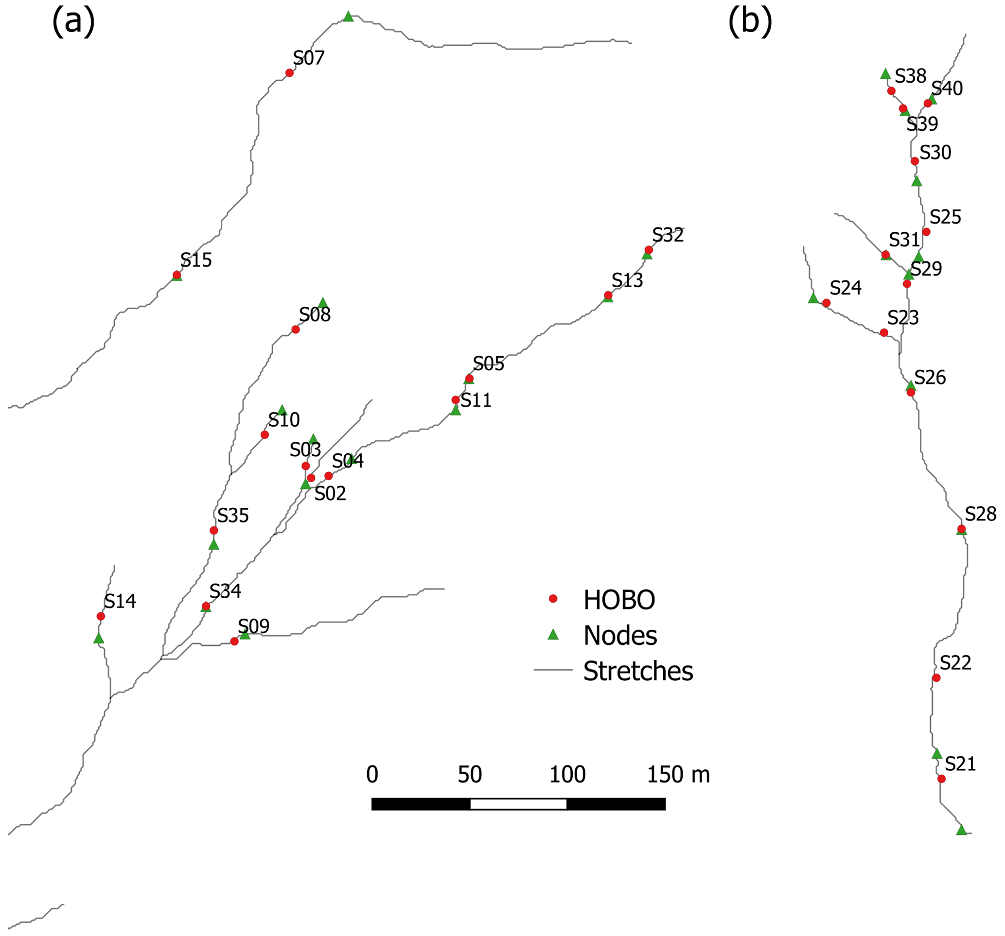
Figure 1 (a) Ortophoto of the Valfredda catchment and its location in northern Italy (green dot), position of the meteorological station (red dot) and the section where discharge measurements were taken (white square). Sensors placed along the tributaries of Zone 1 (c) and Zone 2 (b). The map was generated with Arcgis Pro 2.7.1 (https://www.arcgis.com/index.html, last access: 4 October 2019).

In particular, the test catchment comprises the northern part of the Rio Valfredda, which has a total contributing area of 2.6 km² and is characterized by an average annual rainfall of approximately 1500 mm. Most of the precipitation is concentrated between April and August, while during winter, the catchment is usually covered by snow. Temperatures vary between seasons: in 2019, the minimum was recorded in January (−11.9 ^∘C) and the maximum in July (30 ^∘C). The catchment area spans a wide range of elevations (between 1900 and 3000 m a.s.l) and is characterized by heterogeneous morphological traits. On the upper part of the catchment, deposits of gravel and rocky debris are predominant. These deposits are covered by thin grasslands and ensure a high soil permeability. Below 2100 m a.s.l., trees grow mostly along the streams on a sedimentary bedrock (Durighetto et al., 2020). This heterogeneity of the landscape strongly influenced the observed hydrological dynamics and placed a constraint on the experimental setup of the study.

While the average drainage density of our study catchment (D_d=2.22 km⁻¹) is in line with that of other sites where similar analyses were conducted (Jensen et al., 2018; Botter et al., 2021; Senatore et al., 2021), the internal distribution of the channel network is uneven. The analysis of a high-resolution DTM indicates that the hydrographic network of the upper Valfredda, here seen as the sum of permanent and temporary reaches, directly drains 65 % of the total contributing area (1.7 km² out of 2.6 km²). The remaining 35 % of the catchment, instead, drains into a number of pits located in the central part of the catchment, where water is allowed to infiltrate in the subsurface without generating surface runoff owing to the presence of a fractured bedrock and a karst region. In the central part of the study catchment, there are a couple of localized springs with a seasonally variable discharge that ranges from about 60 L s⁻¹ in late spring to 35 L s⁻¹ in fall. These springs feed a perennial channel with a total length of approximately 1100 m, which constitutes the non-dynamical fraction of the network. The presence of karst areas adds complexity to the hydrological processes responsible for the spatial patterns of surface runoff. Nevertheless, it is interesting to study these kinds of catchments, since karst formations are a quite widespread phenomenon, typical of the southeastern side of the Alps (Jurkovsek et al., 2016) and common also in the USA (USGS, 2020). These landscapes are shaped by the erosion of sedimentary rocks, such as limestone, dolomite and chalks, which are frequently observed in the northeast of Italy, as documented by the geologic map released by the Italian Institute for Environmental Protection and Research (ISPRA, 2022).

For this research, experimental data were collected between 4 September and the end of October 2019, when major snowfall covered the whole landscape and all the sensors. The limited duration of the study period (2 months) is partly implied by the characteristics of the catchment, which is usually covered by snow from early December until the end of spring (June). This per se constrains the maximum duration of the time window available to analyze river network dynamics in the upper Valfredda catchment, as long as the winter season freezes the system for 6 months and renews the underlying stream dynamics.

2.2 Water presence sensors

The dynamics of the active stream network during the study period (September and October 2019) were observed using 31 onset HOBO Pendant loggers (HOBO UA-002-64, Onset Computer Corp, Bourne, MA, USA, hereafter HOBO) suitably modified following the methodology suggested by Chapin et al. (2014). The main changes introduced in this study consisted in removing the light sensor and adding two long electrodes, which recorded a positive electrical signal when connected by the flowing water. The obtained ER sensors were placed along the river network to estimate flow intermittency within different network nodes. The electrical conductivity signal recorded by the HOBOs ranged from 0 to 330 000 lux (corresponding to the maximum value recorded by the sensors when the two electrodes were fully immersed in water) and the temporal sampling resolution was set to 5 min.

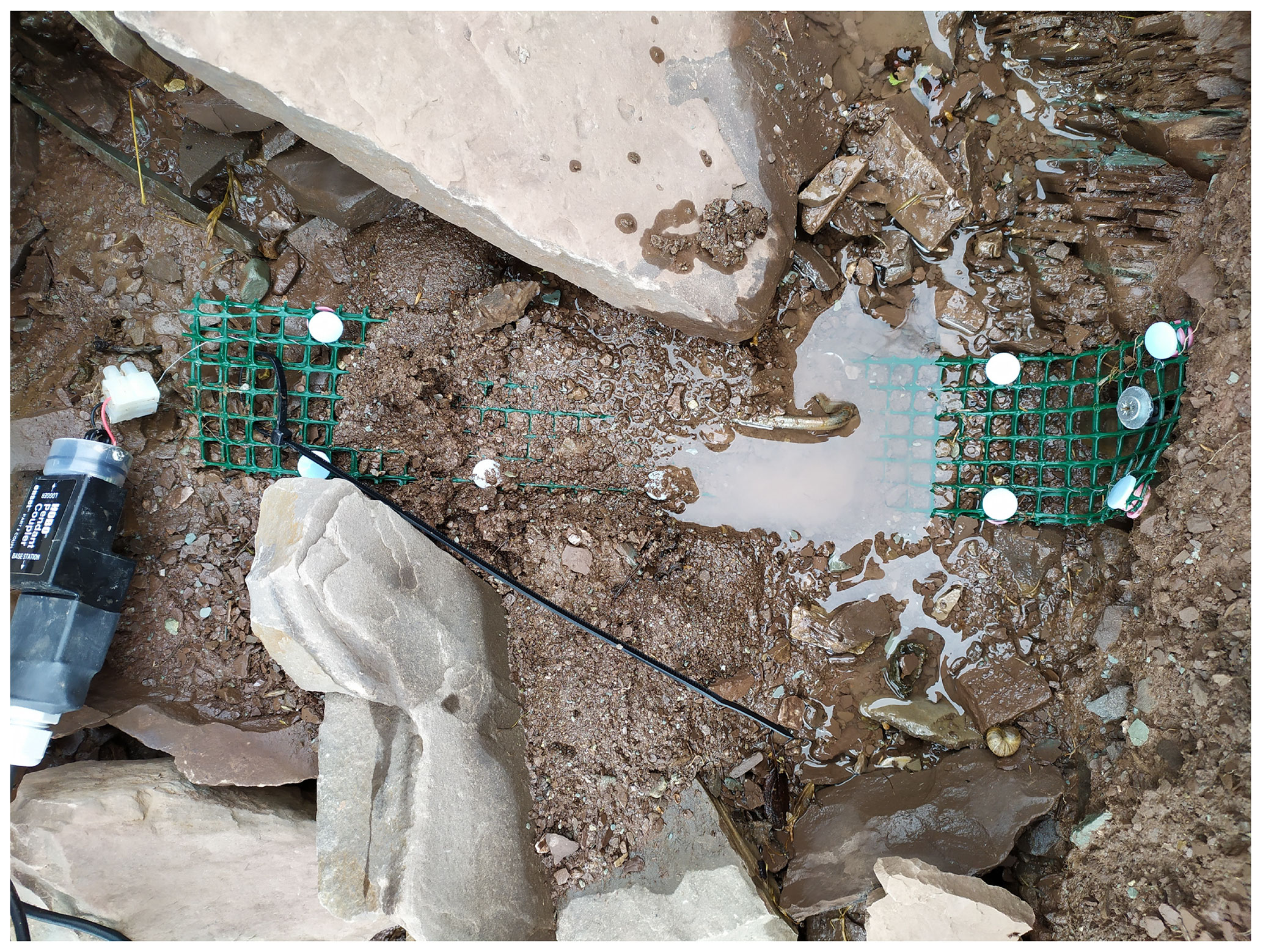
The riverbed of the Valfredda Creek is highly heterogeneous and hydro-morphodynamical variations induced by changes in flow magnitude might cause the flowing water to dodge the sensors, thereby impairing the reliability of the recorded data. To avoid cases in which water flow paths could bypass the sensors, particularly during low-flow conditions, a novel experimental setup was identified, allowing the monitoring of the hydrological state of the whole cross-section where the sensors were placed. The two machine pin electrodes coming out of the sensors' housing cap were connected with two stainless steel wires, from 50 to 100 cm long, rolled up to a geotextile net. The length of the geotextile and wires guaranteed that the entire cross-section of the channel was connected to the sensor, avoiding interference due to possible variations of the flow field. Rolling the cables on the network prevented them from moving when flooded, possibly creating artificial short circuits or bypasses that might impair the reliability of the electrical signal recorded. The net was then attached to another geotextile using plastic buttons to separate the electrodes from the ground by a few millimeters and avoid interference with the wet soil. When placed in field, HOBOs were secured to their networks with suitable plastic strips; furthermore, silicon was used to protect all the sensors' housing caps and prevent infiltration of water within the sensors.

The water presence sensors were installed in mainly two different regions of the test catchment, as shown in Fig. 1. The location of each sensor was chosen based on field surveys carried out prior to the installation of the instruments. Technical difficulties and the time needed to reach each node of the network were carefully considered in the selection process. The specific location of the sensors was also chosen taking into account the heterogeneous substrates of the catchment, so as to enable an accurate analysis of the sensors' behavior in different settings while granting an even distribution of the nodes' persistency (see Sect. 2.3.1). Fifteen sensors were deployed along tributaries of the southeastern part of the basin (Zone 1), an area that has glacial morphogenesis and is characterized by moraine deposits shaped on mild slopes covered by pastures (Fig. 2a); therein, river width ranges from 20 to 80 cm, and the sensors were fixed to the ground using pickets (Fig. 2c). This led to a quite uneven spatial distribution of the sensors, with an average distance between them of approximately 55 m. Thirteen sensors were placed in the northwestern part of the network (Zone 2), where the riverbed is on a steep canyon composed of quartz porphyry rocks (Fig. 2b). These rocks are small, unstable, and can move along the channel in response to rainfall events, thereby supporting the intermittent nature of hydrologic flows. In this region, the channel width ranges from 20 cm to about 1 m, and the sensors' nets were screwed on rock ledges (Fig. 2d). In Zone 2, the criteria used in the selection of the HOBOs' positions were the same as for Zone 1. However, a more even spatial distribution of the ER sensors and a smaller average distance between the probes (30 m) were obtained in this case. The other three sensors were installed along three disconnected branches of the network, on the grassland between Zones 1 and 2. Data collected from the latter sensors were used only for analysis of the underlying network dynamics and not for the statistical analysis of Sect. 3.2, because they experienced very few wet and dry transitions. Some of the tributaries of Valfredda Creek were monitored only through visual inspection, as field surveys allowed a simple, yet reliable, characterization of the hydrological conditions experienced by those reaches during the study period (these tributaries were permanently wet even under extreme low flow conditions, or they were completely dry even during the most intense precipitation event of the entire period). The field surveys are described in the following sections.

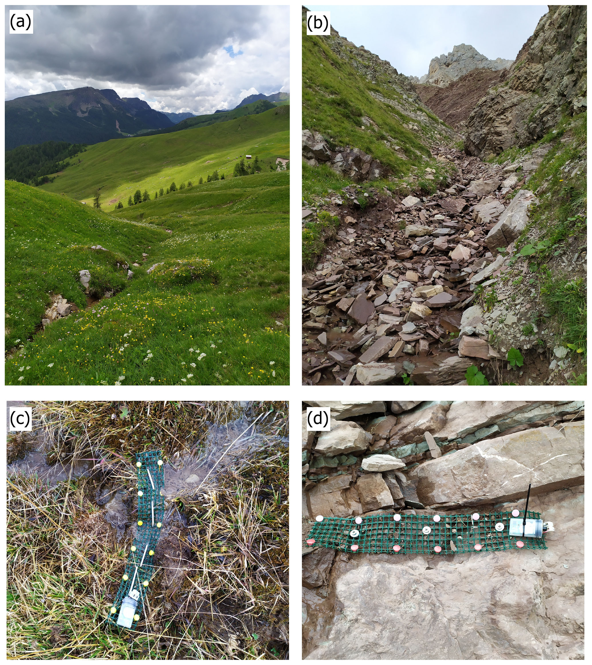
Figure 2 (a, c) Picture of Zone 1 (a) and a sensor on the grass (c). (b, d) Picture of Zone 2 (b) and a sensor net screwed on a rock (d).

2.3 Data analysis

2.3.1 Water presence data and flow persistency

The data collected by the HOBOs were analyzed, and two hydrologically relevant indexes were calculated from the available time series: the average intensity (AI) and the exceedance of the threshold (E). Average intensity is the mean of the electrical signal registered by each HOBO in the period of record. Exceedance of the threshold indicates the probability that the electrical signal registered by a sensor is greater than or equal to a chosen threshold value, ideally separating wet from dry conditions. Different thresholds were initially considered, but the final value (270 000 lux) was chosen based on the intensity measured by the instruments placed in wet nodes during the field surveys. We decided to infer the threshold value directly from field observations instead of relying on laboratory experiments (e.g., with a soil column), to obtain a more reliable representation of the complexity of the natural environments typically found in most headwater catchments of the alpine region. The above hydrological indexes (AI and E) were calculated for each ER sensor and subsequently correlated with the persistency of the corresponding nodes, which was estimated as detailed below.

During the study period, several field surveys were conducted to check the reliability of the signal recorded by the ER sensors, download the data and monitor the status of the network nodes under different hydrological conditions. However, these surveys were not homogeneous in space or systematic in time, thereby making a reliable estimation of the persistency of the network nodes impossible during the study period on a purely experimental basis. Therefore, we decided to estimate the persistency of the nodes using a model that links the spatial configuration of the network to rainfall data, as detailed in the study by Durighetto and Botter (2021). The main model assumptions and its performance in reproducing observed stream dynamics are detailed in Appendix C. The model was calibrated and validated based on 24 complete field surveys carried out for the whole Valfredda catchment from the summer of 2018 to the fall of 2020. During each survey, more than 500 nodes were classified as wet or dry, based on the observed hydrologic conditions of the network (Appendix A). In the light of the good performance of the model (Durighetto et al., 2020; Botter and Durighetto, 2020; Durighetto and Botter, 2021), this was used to estimate the persistency of the nodes (here defined as the fraction of time during which a node was simulated as active in the reference period), exploiting information on the antecedent precipitation accumulated over 5 and 35 d.

2.3.2 Rainfall and discharge data

Discharge measurements were taken in a cross-section at the outlet of the study catchment where water flows permanently. A pressure transducer allowed the measurement of the water stage with a temporal resolution of 5 min. Seven-point streamflow measurements were combined to stage data to estimate the rating curve at the outlet of the catchment with discharges ranging between 9 and 300 L s⁻¹ and a coefficient of determination R²=0.99. Discharge data were collected with a three-dimensional flow tracker under different hydrologic conditions, so as to derive a reliable rating curve. Discharge time series were then derived for the entire study period with a temporal resolution of 3 h, so as to reduce the noise in the recorded signal. The same method was applied to measure the constant discharge originated by the localized springs that feed the permanent fraction of the river network.

To visualize the hydroclimatic dynamics experienced by the study catchment during the focus period, we used rainfall data gathered from a meteorological station that was installed within the basin in 2018 (Fig. 1). The meteorological station is used to monitor precipitation, temperature, relative humidity, net solar radiation and wind speed with a sub-hourly temporal resolution.

2.3.3 Corrections applied to the ER data

A common problem affecting the data recorded by the water presence sensors of this study is that not all the probes could be deployed in the field at the same time. Moreover, several sensors did not work properly during their deployment. In particular, two HOBOs placed on the grass (Zone 1) – where water flow was not observed permanently, as the channel activated only during and after precipitation events – exhibited a tendency to silt, while others were found detached from their geotextile nets because of the presence of several horses grazing in the area. In Zone 2, debris flows triggered by precipitation prompted the accumulation of wet sediments around the geotextile, altering the signal recorded by the electrodes of a probe placed along the rock canyon. Thus, for both these reasons, there were many missing data in the time series that had to be dealt with. In Appendix B, we describe all the corrections that were applied to the data to take into account the lack of synchronicity of the available water presence data and the technical problems encountered during the deployment.

2.4 Spatial and temporal dynamics of the active network

A visual representation of spatial and temporal dynamics of the river network was obtained based on the intensity signal recorded by the HOBOs, as detailed below. At each time step, the electrical signals recorded by each sensor and its neighbors were interpolated in space, in order to define which part of the stretch connecting the nodes was wet or dry. The threshold value of the electrical signal used to determine the wet or dry status of the stretches was 270 000 lux, as detailed above (Sect. 2.3.1). Probes were divided into three categories, depending on the electrical signal recorded:

• Active, when the value of intensity was greater than the threshold, and the cross-section where the HOBO was placed was identified as wet.

• Inactive, when the signal collected was lower than the threshold, and the cross-section was identified as dry.

• Missing data, in the case of no data and zeros induced by malfunctioning of the sensors (Sect. 2.2).

We identified a river stretch as a reach connecting two subsequent HOBOs. When two neighboring sensors were both active, inactive or missing data, the stretch in between was defined as active, inactive or missing data accordingly. In contrast, if two neighboring HOBOs had data, but one of them was active and the other was inactive (or when a sensor with missing data had two neighboring HOBOs providing reliable data), the wet length in the stretch connecting those sensors was calculated using a linear interpolation of the electrical signal measured by the nearest probes. Whenever a stretch had both missing data sensors at its end points, and it was located between two concurrently active or concurrently inactive stretches, it was classified as active or inactive accordingly. In contrast, if a stretch with missing data was located between two stretches with a different status (i.e., one active and one inactive), it was plotted as a stretch with missing data – as the available data did not allow a proper identification of the status of the sensors and the location of the wet/dry transition. This method could not be applied to stretches classified as missing data if they were located at the sources or in presence of confluences. In these cases, the behavior of the neighboring stretches, experimental evidence and the observed spatial patterns of persistency were considered in order to define the status of the stretch (active, inactive or missing data). Finally, a time-lapse visualization of the stream network dynamics with a temporal resolution of 3 h was obtained using a MATLAB code.

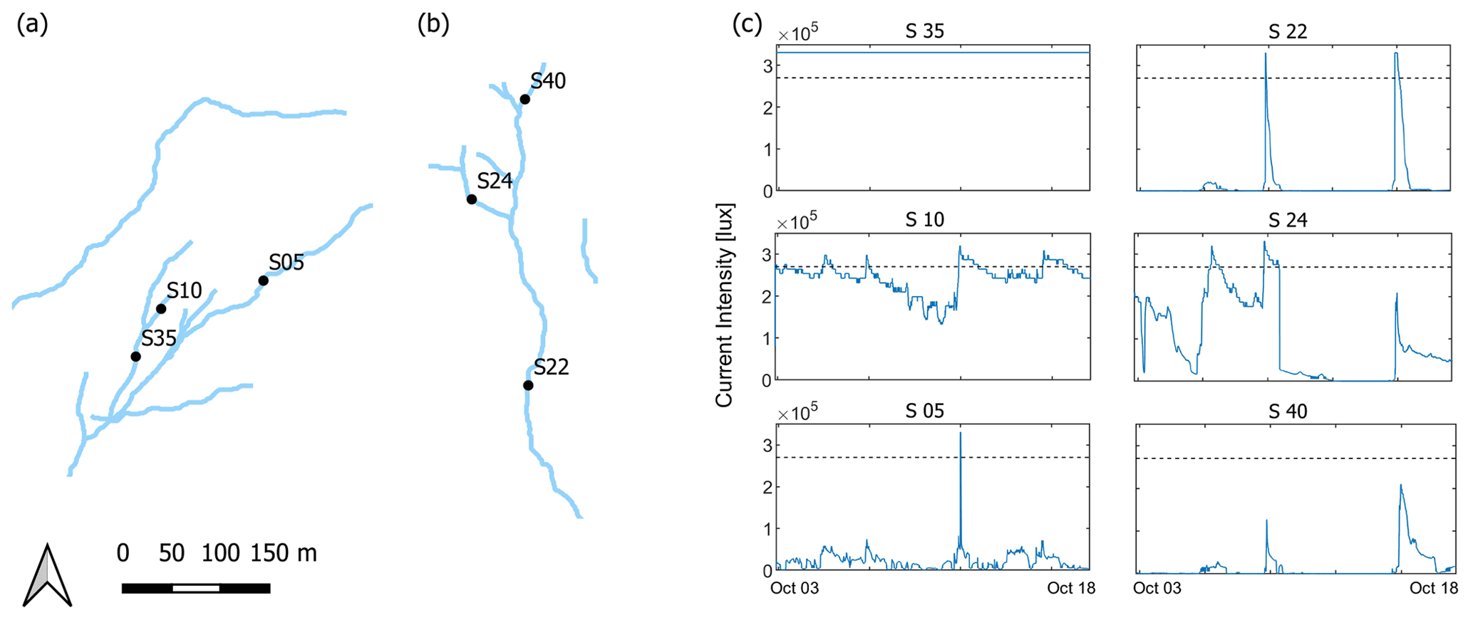
Figure 3 Examples of time series recorded by some of the sensors for 2 weeks between 3 and 18 October. Location of these sensors along the tributaries of Zone 1 (a) and 2 (b). The dashed line represents the threshold of 270 000 lux (c).

2.5 Active length vs. discharge power-law model

Catchments can be seen as dynamical systems where the discharge at the outlet and the active length co-evolve in time, in response to the underlying climate forcing. In this study, we seek to use high frequency ER data to evaluate the robustness of an empirical model often proposed in the literature, linking the wet length and the corresponding discharge using a power-law relationship (Godsey and Kirchner, 2014; Jensen et al., 2017; Lapides et al., 2021):

$$\begin{array}{}\text{(1)}& L=a{Q}^b.\end{array}$$

Operationally, the analysis was performed as follows. Logarithms of synchronous observations of L and Q were plotted in a Cartesian plane, and a linear regression was applied to the data. The equation of the interpolating line corresponded to the linearization of the power-law model:

$$\begin{array}{}\text{(2)}& \log \left(L\right)=\log \left(a\right)b\log \left(Q\right).\end{array}$$

The parameters log (a) (vertical intercept) and b (slope) were first calculated for the whole set of available L and Q data with a temporal resolution of 3 h, and the goodness of fit of the linear regression to the data was evaluated through the coefficient of determination, R². A resampling procedure was also used to analyze how the parameters of Equation (1) and the goodness of fit of the linear regression depend on the temporal resolution of the available data (Appendix D).

3 Results

3.1 Time series of water presence and electrical resistance

In most cases, the time series of the electrical signals recorded by the sensors placed in the field, I(t), show a pronounced temporal variability within the whole period of record. The analysis of the time series of the electrical signals recorded by the HOBOs elucidates the different hydrological behavior of the two study zones and also emphasizes the heterogeneity of the signal recorded by different sensors within each zone.

The HOBOs belonging to Zone 1, which were all placed on a grassy substrate, exhibited quite heterogeneous behavior. Some sensors, such as S₃₅ (Fig. 3), systematically recorded intensity values close to the maximum intensity, as they were located along streams where water flowed permanently during the entire study period. Other sensors, instead, were placed in more dynamical streams and displayed an electrical signal that fluctuated between the maximum intensity (during rainfall events) and 100 000–150 000 lux (during the driest periods: S₁₀). Other sensors, mainly located in the higher part of Zone 1, recorded no intensity at all during most of the time, with intensity peaks over the threshold that were observed only during rainfall events, when discontinuous ephemeral ponds were generated in correspondence of the stream network (S₀₅).

Unlike the HOBOs of Zone 1, none of those placed in Zone 2 (Fig. 3) was consistently wet during the whole study period. The probes activated during rainfall events and dried out afterwards with heterogeneous velocities, depending on their position: sensors located in the central part of the creek persisted being wet for longer (see, e.g., S₂₄), while those placed close to the channel heads turned off very quickly after each rain event (S₂₂). Other sensors, while they recorded an increase in the electrical signal during precipitation events, remained consistently below the 270 000 lux threshold for the entire study period (S₄₀).

3.2 Statistical analysis

A statistical analysis was carried out to assess the consistency between the hydrologically relevant indexes (namely, the average intensity and the exceedance of the threshold) calculated for each sensor and the persistency of the corresponding nodes, as derived from field surveys (Sect. 2.3.1). Figure 4 shows the scatter plots of persistency vs. AI and persistency vs. E for 28 sensors of Zones 1 and 2. All the available data were represented in the same two plots in order to emphasize differences and similarities among the HOBOs located in different zones.

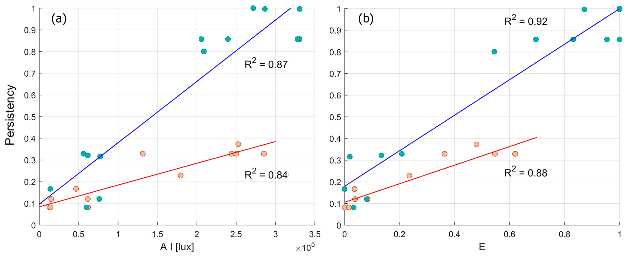
Figure 4 Scatter plots of persistency vs. average intensity (a) and persistency vs. exceedance of the threshold (b) of the sensors of Zone 1 (green points) and Zone 2 (orange points).

We hypothesize that a higher persistency of the nodes is reflected by a higher average intensity of the current recorded by the sensors and an enhanced probability that the electrical signal exceeds the selected saturation threshold. These hypotheses seem to be supported by the high coefficients of determination that were calculated from the data (R² always above 0.84). However, Fig. 4 also shows that the morphological characteristics of the zones studied (altitude and heterogeneous land cover) can influence the electrical signal registered by the instruments. Data collected from sensors of Zone 1 are not homogeneous, despite being located close-by in the field. The HOBOs of Zone 1 are clustered in two separate groups (Fig. 4): one cluster includes the sensors located downstream, which are mostly wet (E>0.7 and $\mathrm{AI}>\mathrm{2}\times {\mathrm{10}}^{\mathrm{5}}$ lux), and the other includes the HOBOs located upstream, that turn on only during rainfall events (E≤0.2 and $\mathrm{AI}<\mathrm{0.8}\times {\mathrm{10}}^{\mathrm{5}}$ lux). Instead, the tributary where the sensors of Zone 2 are located dries down completely, as indicated by the low value of the maximum persistency observed in this area. The data points in these cases are evenly distributed along the regression line, indicating a more homogeneous internal distribution of node persistencies. It is also interesting to note that the two zones display very heterogeneous regression slopes between mean intensity and persistency. In contrast, the slopes of the regression lines between exceedance of the threshold and persistency are comparatively more similar in the two zones. This suggests that E might be a more robust indicator of the underlying hydrological dynamics experienced by the nodes in the network, regardless of the specific position of the sensors in the catchment.

3.3 Stream network dynamics

Data collected by the sensors deployed along the watercourse provided information regarding the high-frequency spatial and temporal dynamics of the stream network. The full video of the observed river network dynamics is shown in the video supplements, while the main text presents a sequence of snapshots taken from the video that represent the temporal evolution of the spatial configuration of active channels in the study catchment (Fig. 5). Figure 5a represents the channel network during the most intense rainfall event of the study period, on 8 September, when all of the sensors of Zone 1 (left) were wet (blue dots). Not all the sensors of Zone 2 (right) had been installed at that time. This circumstance explains the reason why some stretches are represented as no data (white dots) in that region. Nonetheless, on 8 September most of the network streams were wet also in Zone 2, with the exception of two river segments (shown in orange) that remained dry during the entire study period.

After the rainfall event that was observed on 8 September 2019, the network kept drying out for several weeks and then wetted up again, owing to a rain event that was observed on 25 September (shown in Fig. 5b). This precipitation event was less intense than the previous one, and it was characterized by a lower antecedent precipitation. Consequently, some headwater branches in both zones did not get wet.

The snapshot in Fig. 5c shows the network on 5 October, 3 d after an isolated precipitation event that took place during a relatively dry period. On that date, all the HOBOs of Zone 2 were dry, while only the downstream sensors of Zone 1 (those closer to the permanent part of the network) became wet. Figure 5c once again emphasizes the dynamical nature of the channel network in the study catchment and the different hydrological behavior of the two focus regions identified in this study.

Figure 5 Map of the active stream network of Zone 1 (left column) and Zone 2 (right column) on 8 September (a, d), on 25 September (b, e) and on 5 October (c, f). Active stretches and sensors are blue, inactive ones are orange and no-data elements are white.

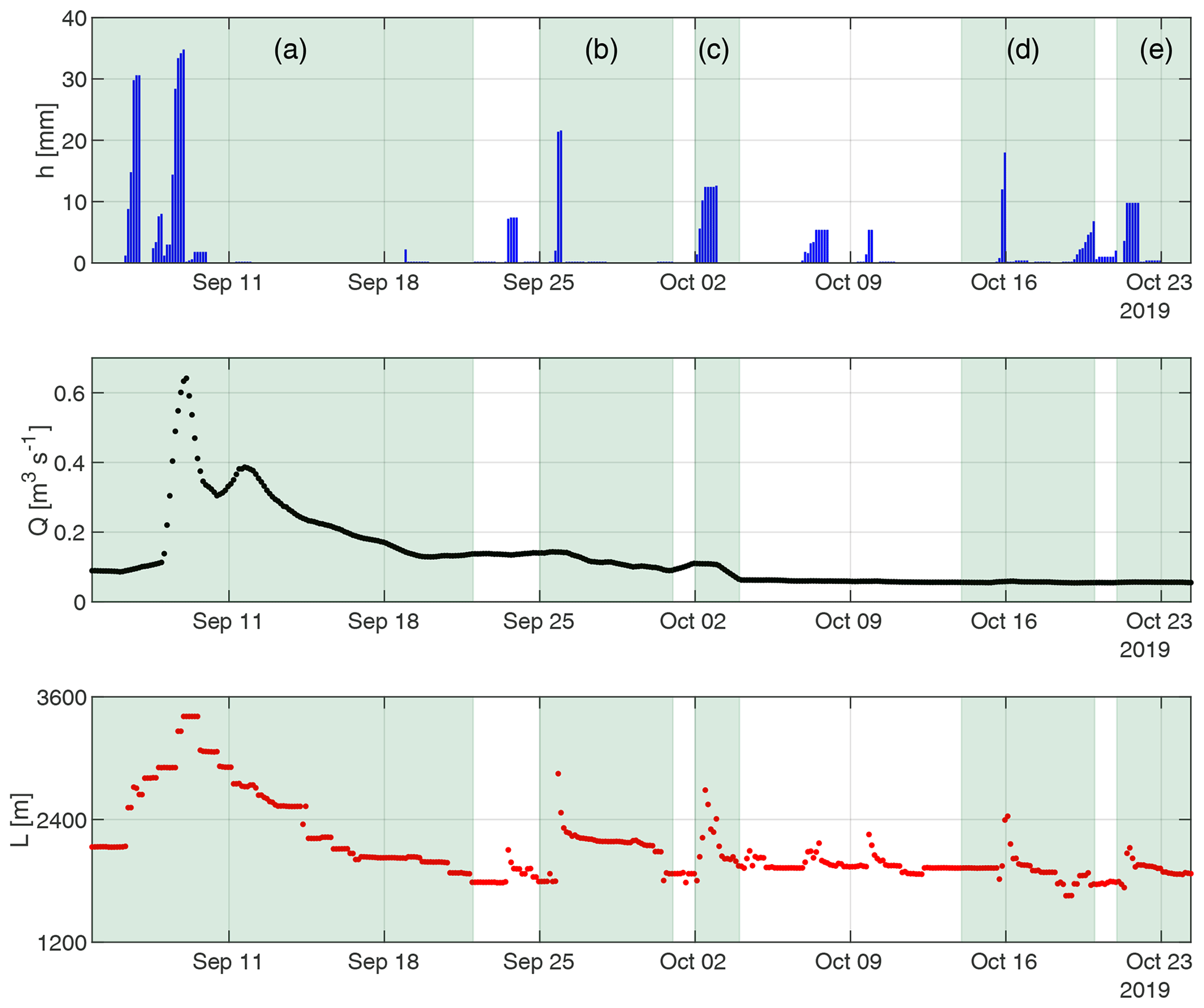
Figure 6 Top panel: temporal evolution of rainfall during the study period. Center panel: temporal evolution of catchment discharge, Q(t), during the study period. Bottom panel: temporal dynamics of active length, L(t), during the study period. Areas in green represent the periods during which active length and discharge are plotted in Fig. E1.

3.4 Active length–discharge relationship

The temporal evolution of rainfall (h), total discharge and total active length during the entire study period is shown in Fig. 6. During the first precipitation event, the most intense of the period, observed variations of Q and L were both significant. After 11 September, instead, the intensity of the events was smaller and discharge variations were less important. However, ER sensors indicate that small rainfall volumes were able to activate several channels for some days, leading to noticeable changes in the total wet length L. Overall, the figure indicates that the dynamics of L were mainly driven by precipitation, the temporal pattern of which differs from the corresponding streamflow dynamics.

Figure 7 summarizes the joint changes of wet length and discharge during the whole study period. The variations of Q caused by the first precipitation event (blue dots) are larger than those observed in the remainder of the period. Instead, active length dynamics are observed during the entire study period. The available data of Q and L were fitted with a power-law relationship, of the type shown in Eq. (1). While we found that log (L) and log (Q) are linearly correlated (Fig. 7), we also observed some scatter of the points around the regression line (R²≃0.5), which is due to intra and inter-event changes in the responsiveness of Q and L to the underlying rainfall forcing. The exponent of the power-law model, b, is close to 0.2, which is a relatively low value but still falls within the range given in the literature (Godsey and Kirchner, 2014; Prancevic and Kirchner, 2019). The high-frequency data gathered in this study allowed us to analyze the relationship between catchment discharge and active length also during individual rain events, discussed in Appendix E.

Figure 7 Plot of total discharge (Q) and total active length (L).

4 Discussion

Our customized version of water presence ER sensors was successfully deployed in the field in two different regions of the Valfredda catchment, which are characterized by heterogeneous substrates and different types of riverbed. The sensors proved to be reliable in recording the hydrologic conditions of the whole cross-section where the sensors were placed, especially during low-flow conditions, when the observed stages were very low, and the flow field was spatially heterogeneous and irregular within many cross-sections. Nevertheless, our study indicates that water presence sensors require particular caution during their deployment in the field and the interpretation of the field data. The major issues that were faced during the deployment changed based on the location where the HOBOs were placed: in the portion of the network dominated by debris (Zone 2), ER sensors were prone to be covered by sediments or flushed away by the flow field; conversely, in other regions of the network where the substrate was made by a thin organic soil covered by grass (Zone 1), the main problems were represented by grazing animals and the formation of local pools with standing water during the drying of the network that could not be distinguished from flowing stream in the ER time series. In addition, in both regions, there were issues related to the fragility of the steel cables and/or the sealing system used to protect them from water infiltration during floods. Thus, intensive field surveys were necessary to check the functioning of the sensors and repair possible damage during the study period.

The high sampling frequency set for each instrument (5 min) and the large number of sensors used (more than 30 sensors for a maximum network length close to 2 km) allowed us to reconstruct maps of the active stream network with a high spatio-temporal resolution. A similar result could not have been obtained through visual inspections of the catchment. The low cost of the HOBOs and their long-lasting batteries support their potential to monitor active network dynamics in a wide range of contexts. However, when planning the use of these sensors, it should be taken into account that some probes can be damaged or lost during the deployment and data acquisition, creating frequent gaps in the time series available.

Our data suggest that the two regions of the study catchment are strongly heterogeneous, not only in terms of land cover but also in many features of the underlying network dynamics. The lower part of Zone 1 was permanently wet, with high values of E and persistencies close to 1 for most of the sensors. In the upper part of the same zone, instead, the network branches were more dynamical, and they usually became wet in response to precipitation events. Along the main channel of Zone 2, instead, water was able to infiltrate and exfiltrate rapidly, creating frequent stream disconnections promoted by the unstable morphology of the riverbed. In this case, mean current intensities and node persistencies were consistently smaller than those observed in Zone 1.

In both regions, we found a good correlation between the persistency of the nodes and two statistical features of the electrical signal recorded by the ER sensors (namely, the mean intensity and the exceedance of a suitably selected saturation threshold). This suggests that the statistics of the ER signals recorded in the field could be robust indicators of the hydrological status of different network nodes. In particular, ER time series could be used to extrapolate information on the spatial patterns of node persistency, which could, in turn, be used to define the hierarchy according to which the nodes in the network are activated in response to rain events and then deactivated during the subsequent drying (Botter and Durighetto, 2020).

Our data indicate the presence of some hysteresis in the active length vs. discharge relationship at fine temporal resolution, especially during low-flow conditions (Fig. 7). Network length was found to be more sensitive than discharge to small precipitation inputs: while most rain events induced visible changes in the active channel length, the catchment streamflow was sensitive only to rain events lasting for several consecutive days (6–9 September, 13–18 October, 20–24 October) and to intense storms (more than 20–30 mm in 9–12 h). In particular, when rain events were moderate, the channel network activated, but the amount of water conveyed to the outlet was limited, owing to network disconnections and limited flow velocities; conversely, when rain events were more intense, the same active length contributed a much larger discharge to the outlet. Interestingly, in this case, the use of a bijective L–Q function to infer active length changes from discharge variations would underestimate the observed standard deviation of the active length by 35 %. It is worth noting that while some scatter in the L vs. Q plots has been already observed in the literature (Jensen et al., 2019; Senatore et al., 2021), caution should be placed in generalizing our results. In fact, the Valfredda catchment is a high relief catchment with several temporary and permanent disconnections in the channel network and a marked spatial variability of geologic substrate and stream persistency. All these factors might possibly contribute to enhance the non-linearity of the hydrological response of the Valfredda, thereby preventing the emergence of a clear one-to-one relationship between total active length and catchment discharge in this specific case.

5 Conclusion

In this work, we tested the use of ER sensors for the monitoring of active network dynamics in a high-relief 2.6 km² catchment of the Italian Alps during the fall of 2019. To this aim, we utilized a customized version of the HOBO sensors previously proposed in the literature, which was modified to be suited for a deployment under different substrates and is deemed to be more accurate under unstable hydrodynamic conditions and during low-flow conditions. The following conclusions are worth emphasizing:

• ER sensors provided valuable information about high-frequency, space–time network dynamics in the study catchment during the fall of 2019; in particular, the ER data collected were used to produce a video and a sequence of maps representing the dynamics of the active network with a sub-daily temporal resolution.

• The mean intensity of the ER signal and the exceedance of a suitably selected intensity threshold were found to be highly correlated with the persistency of the network nodes. This suggests that ER signals provide statistically meaningful information on the hydrologic status of different nodes of the river network.

• The successful application of ER sensors under the heterogeneous environmental conditions found in the Valfredda catchment suggests a good potential and flexibility of the tool for river network mapping. Likewise, the study highlighted the major shortcomings of this type of technology and the dependence of these shortcomings on the type of substrate: in steep rocky channels, the main problem is the sensor flushing during floods and the accumulation of sediments; in grassy regions, the major problems relate to water ponding and grazing of animals, which might remove the sensors during the deployment. For the above reasons, we propose that the use of ER sensors for river network mapping needs to be quite intensively supervised.

• The high-frequency monitoring of active stream lengths and flow rates performed in this study allowed an analysis of the co-evolution of active length and catchment discharge in response to a sequence of rain events. Our data highlighted the larger responsiveness of the active length to small rain events and evidenced non-synchronous variations of L and Q at sub-daily time scales during the 2 months of field campaign performed in this study.

It is fair to stress that a longer dataset could further enhance the robustness of our results, as new events could be included in the analysis. This, however, would require significant efforts, especially in the light of the challenges imposed by the specifics of the site (e.g., the heterogeneous substrate, snow dynamics, the high frequency of floods and the presence of grazing animals, which might interfere with the sensors). This is deferred to future work.

Appendix A: Flow persistency

A conventional criterion was identified in order to classify the nodes as wet or dry along the intermittent tributaries of Valfredda Creek during surveys in the field: if the streamflow had a width equal to or greater than 10 cm, the node was considered as wet (otherwise the node was identified as dry). This lays at the basis of all the calculations of active network lengths and the persistencies of the nodes, as detailed in Appendix C. The analysis of the persistency of the nodes along the tributaries helped in the selection of the position of the HOBOs. This position was identified so as to guarantee a reliable representation of the underlying stream network dynamics (Fig. A1). In doing that, a one-to-one association between the ER sensors and specific network nodes was established.

Figure A1 Nodes and corresponding sensors of the tributaries of Zone 1 (a) and Zone 2 (b).

Appendix B: Corrections applied to the data

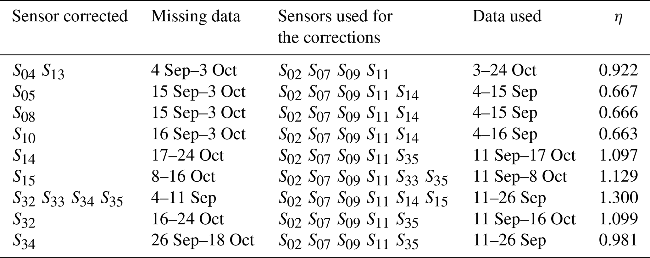
To account for missing data, weights (η) that relate the probability of exceedance of the threshold of all the active sensors of a zone to the exceedance of the threshold of a sensor during a period of time containing missing data were calculated (Tables B1 and B2).

The ratio between the probability of exceeding the threshold of a sensor during the period t_A, when it is not active, and t_B, when it is functioning, is assumed to be equal to the ratio between the mean probability of exceeding the threshold of all the other active sensors of the zone during $t_A\left(P_{t_A}\right)$ and $t_B\left(P_{t_B}\right)(\mathit{\eta }$).

$$\begin{array}{}\text{(B1)}& \mathit{\eta }={\displaystyle \frac{P_{t_A}}{P_{t_B}}}.\end{array}$$

During rainfall events, some of the sensors were buried by sediments, but they kept measuring 330 000 lux as if they were completely wet even when there was no longer any water flowing on the channel. Their time series were reconstructed based on those of the closest sensors not affected by sediment dynamics.

Table B1 Corrections applied to some of the HOBOs of Zone 2.

Table B2 Corrections applied to some of the HOBOs of Zone 1.

In some parts of the tributary of Zone 2, the channel bedrocks were particularly fragile and unstable, and this prompted the movement of debris along the channel and their deposition between a sensor and its geotextile network. In the upper part of Zone 2, sensor S₃₉ was subject to frequent sediment depositions. During one of the surveys, it was found covered by debris (Fig. B1), and the luminous intensity that it registered was 330 000 lux, as if it was completely wet even though there was no flowing water at the time. After cleaning the sensor (on 7 October), the measured value of electrical current dropped drastically and, as shown by the time series (Fig. B2), the intensity recorded by the sensor remained low until the following rainfall event (9 October).

Figure B1 Sensor S₃₉ covered by sediments.

The temporal dynamics of the electrical signal in the periods from 26 September to 7 October and from 17 to 18 October were reconstructed based on the time series of sensor S₃₈, not affected by sediment dynamics and close to S₃₉. The recession rate with which the signal of S₃₈ declines after a rainfall event was estimated, and that same rate was applied to S₃₉ (Fig. B2).

To correct the asynchronicity between the electrical signals recorded by the sensors and the persistencies of the corresponding nodes the model developed by Durighetto et al. (2020), Botter and Durighetto (2020) and Durighetto and Botter (2021) was applied. It links the spatial configuration of the network to weather data, and here it was applied to estimate the persistency of the nodes between 4 September and 24 October 2019, knowing rainfall heights of that same period as well as the persistencies and precipitation data collected between July 2018 and January 2019 used to develop the model (Fig. C1).

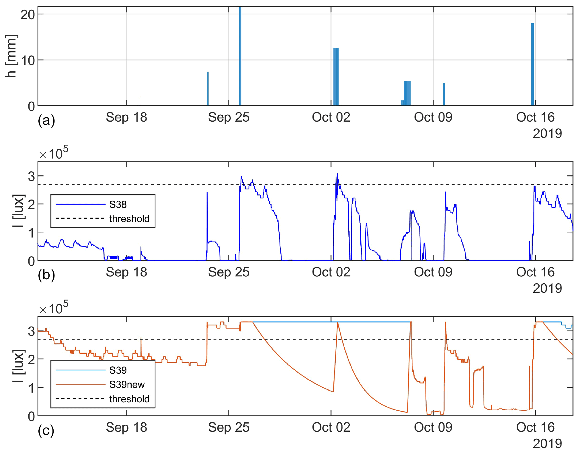
Figure B2 (a) Hyetograph of the period during which the corrections to S₃₉ were applied. (b) Time series of S₃₈. (c) Time series of S₃₉ before the corrections (light blue) and after the corrections (orange).

Appendix C: Empirical model for local persistency

The local persistency of each node during the study period (4 September to 24 October 2019) was estimated by means of the field surveys carried out in 2018 and 2020 and the models described in Durighetto et al. (2020), Botter and Durighetto (2020) and Durighetto and Botter (2021). The procedure is composed of three steps. In the first step, the active length is estimated from antecedent precipitation via the equation:

$$\begin{array}{}\text{(C1)}& L\left(t\right)=k_{\mathrm{0}}+k_{\mathrm{5}}{h}_{\mathrm{5}}\left(t\right)+k_{\mathrm{35}}{h}_{\mathrm{35}}\left(t\right),\end{array}$$

where L(t) is the active length, h₅(t) and h₃₅(t) are the antecedent daily precipitation accumulated over 5 and 35 d, respectively, and k₀, k₅, k₃₅ are calibrated regression coefficients. The daily precipitation was measured by a weather station of the Veneto Region Environmental Protection Agency (ARPAV), located 4.5 km far from the catchment centroid. The coefficients were calibrated on the 9 field surveys carried out during 2018 (mean absolute error = 1.1 %) and validated with the 13 field surveys of 2020 (MAE = 3 %). The simulated active length and the corresponding field surveys are shown in Fig. C1 (for more information, the reader is referred to Durighetto et al., 2020).

The second step consists in simulating the spatial patterns of the active network, starting from the active length. This was accomplished exploiting the hierarchical model of network activation introduced by Botter and Durighetto (2020). The hierarchical model states that, during network expansion, nodes are activated in a given order (from the most persistent to the least persistent nodes in the network) and deactivated in the reverse order during network contraction. Botter and Durighetto (2020) proved the robustness of this model in the Valfredda catchment (average F₁ score equal to 0.98). The specific order of node activation (and, thus, the hierarchy of the nodes) was identified from the field surveys. Then, for each day of the study period, the active nodes were determined by combining the hierarchical model and the empirical model for the active length.

In the third and last step, the local persistency of each node was calculated as the fraction of time for which that node was active during the study period.

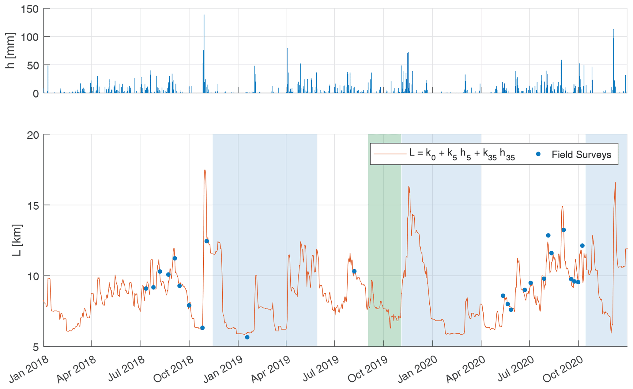
Figure C1 Time series of daily precipitation h, and the corresponding active length L estimated by the empirical model in Durighetto et al. (2020). Blue dots show the 24 field surveys carried out on the catchment. The blue shade identifies periods with snow cover, while the green shade highlights the period during which the ER sensors were employed.

Appendix D: Resampling of the collected data

The resampling of the data was an attempt to reproduce a fictitious sampling campaign with sporadic measurements of active length and discharge, assuming that a standard power-law was applied to the sampled data, as was typically done in all previous studies where the relationship between Q and L was studied (Godsey and Kirchner, 2014; Jensen et al., 2017; Lovill et al., 2018; Prancevic and Kirchner, 2019). First, we subdivided the study period into non-overlapping sub-periods with a constant duration equal to T days and we extracted a single random date and time within each sub-period. Then, the values of Q and L observed during the extracted set of dates and times (one pair for each period with length T) were selected from the available time series of discharge and active length. The linear regression given by Eq. (2) was applied to the resampled Q and L data in order to calculate the corresponding values of R² and b. The random extraction was repeated 50 times, and the mean value and the standard deviation of R² and b (〈R²〉 and 〈b〉, respectively), were calculated. All the above operations were repeated using different values of T: 1, 2, 4 and 7 d.

Figure D1 shows the mean values of b and R² (and the corresponding standard deviations) as a function of the mean sampling interarrival, T. The variations of the mean slope of the regression exponent, 〈b〉, is not significantly impacted by the specific sampling strategy adopted (Fig. D1a). The standard deviation of b instead increases with T, but even at weekly timescales, the observed intersample variations of b are not huge (±30 % for T=7 d), suggesting a certain stability of the exponent of the power-law model. The moderate variations of b observed across different samples with various mean sample frequencies were not expected in the light of the pronounced scattering of the points in the Q vs. L points of Fig. 7. We attributed this behavior to the fact that the scattering in the L vs. Q relationship is particularly enhanced during individual events. Nevertheless, when a set of (L, Q) points belonging to different events is considered (which corresponds to select a set of points with different colors in Fig. 7), they are interpolated by a power-law model with an exponent that does not change dramatically if the specific dates of the sampled points are modified.

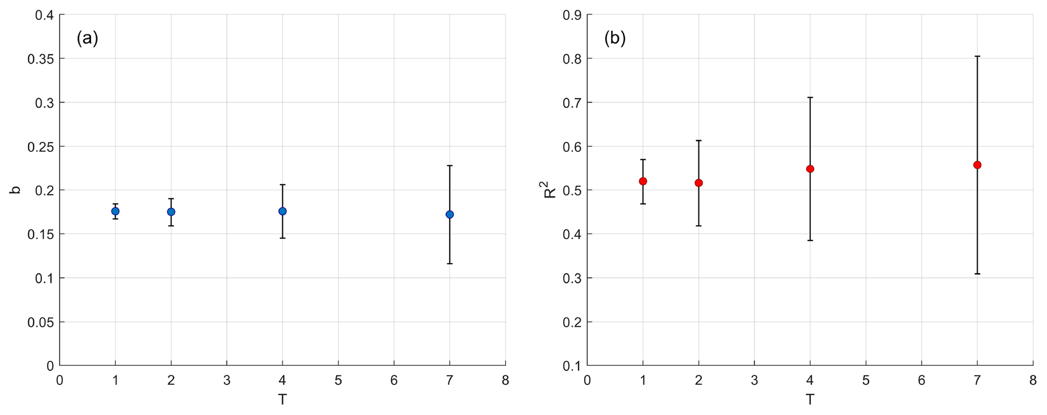
Figure D1 Plot of resampled b (a) and R² (b) mean values and standard deviations as a function of the mean frequency of the resampling T calculated for total active length (L) and discharge (Q).

Our analysis also suggests that when the frequency of the data is low, the hysteresis in the L vs. Q relationship are on average similar to those observed at higher temporal resolutions, as shown by the pattern of 〈R²〉 vs. T in Fig. D1b. Nevertheless, when the mean interarrival between the observations increases, the variability across the samples is more pronounced, and the chances that the experimental (L,Q) pairs do not exhibit a clear power-law trend also increase, as shown by the growth of the standard deviation of R² with T (about 50 % of the mean for T=7 d). This shows, as statistics suggest, that the goodness of fit of the power-law model can be strongly dependent on the specific timing of the field surveys in which active length and discharge are evaluated, making the observed pattern of 〈R²〉 poorly informative.

To conclude, the exponent of the power-law relationship between catchment discharge and total active length was found to be relatively stable in the case of changes of the underlying sampling frequency, which instead had a larger impact on the goodness of fit of the power-law model. When the frequency of the data is lower, the scattering in the L–Q plane is highly sensitive to the specific times during which L and Q observations are taken.

Appendix E: Analysis of the L–Q relationship for single events

Figure E1 shows the joint changes in active length and catchment discharge observed during the five periods shaded in green in Fig. 6.

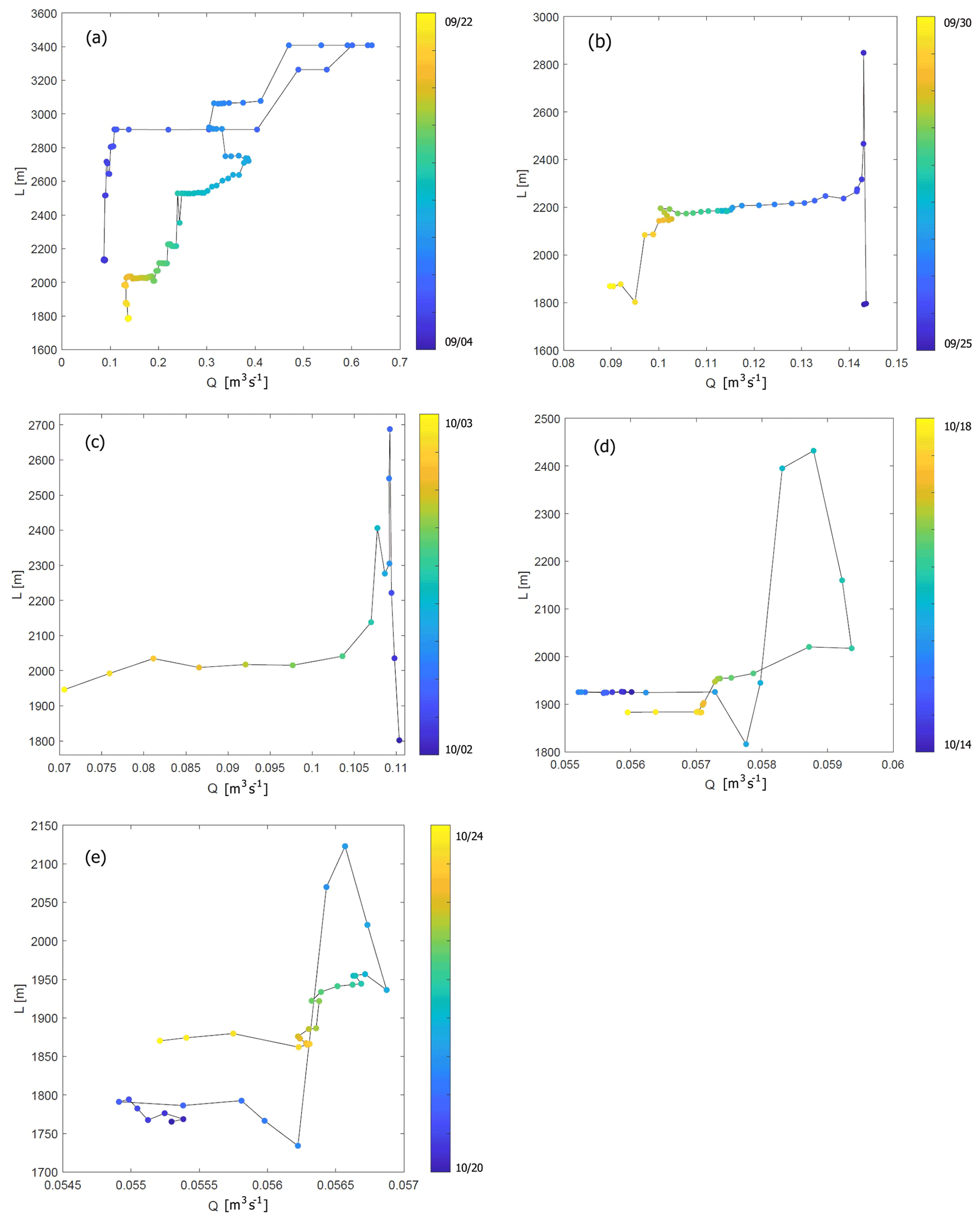
Figure E1 Plots of discharge and active length during individual events across the study period, as indicated in Fig. 6.

During the most consistent precipitation event of the period (8 September), the peaks of active length and streamflow were reached at the same time (Fig. E1a). However, during the early recession of Q, the active length remained stable and close to its peak value. Afterwards, the discharge showed a non-monotonic behavior with a small second peak, while L decreased consistently.

During the precipitation events that took place between 25 and the 30 September (Fig. E1b), and between 2 and 3 October (Fig. E1c), the maximum active length was reached a few hours after each rain pulse – although in the absence of significant Q variations. Afterwards, the wet length first experienced a rapid decrease (again without significant changes in the discharge), and then it remained almost steady while the discharge kept decreasing. A rainfall event preceded the event shown in Fig. E1b, and it was responsible for the increase of the catchment moisture conditions at the beginning of the considered event. Therefore, after the end of the rainfall input, the active length remained stable for some time before it started declining. The trend observed during the event that occurred between 2 and 3 October (Fig. E1c) is similar to that shown in Fig. E1), but in this case, the soil was drier before the event, and the precipitation was less intense, thereby inducing a quicker decrease of the active length as compared to what observed in the recession between 25 and 30 September. In both cases, however, consistent variations of the wet length (ΔL≃1 km) corresponded to comparatively small variations of the discharge (ΔQ≃50 L s⁻¹).

The rain events that took place between 14 and 18 October (Fig. E1d) and between 20 and 24 October (Fig. E1e), instead, exhibited a different trend: the maximum wet length preceded the maximum discharge that was reached only when the active length was almost back to its initial value. In both these cases, the intensity of the rainfall events was small, and the variations of Q were barely noticeable (ΔQ≤5 L s⁻¹).

To summarize, within a single intense rain event, the hysteresis in the L vs. Q relationship depended on the fact that the active length increased more quickly than Q in the early stages of the event, while it decreased much more slowly than Q in the recession. In contrast, the hysteresis across different events was generated by shifts in the sensitivity of Q and L to different types of rain events. In particular, the same active length corresponded to different amounts of water conveyed to the outlet, depending on rain events intensity, network disconnections and flow velocities (e.g., 11 September: L=2900 m Q=338 L s⁻¹; 26 September : L=2900 m Q=143 L s⁻¹).