the Creative Commons Attribution 4.0 License.
the Creative Commons Attribution 4.0 License.
 | 07 Jul 2022
A comparison of hydrological models with different level of complexity in Alpine regions in the context of climate change
Francesca Carletti
Adrien Michel
Francesca Casale
Alice Burri
Daniele Bocchiola
Mathias Bavay
Michael Lehning
This study compares the ability of two degree-day models (Poli-Hydro and a hybrid degree-day implementation of Alpine3D) and one full energy-balance melt model (Alpine3D) to predict the discharge on two partly glacierized Alpine catchments of different size and intensity of exploitation, under present conditions and climate change as projected at the end of the century. For the present climate, the magnitude of snowmelt predicted by Poli-Hydro is sensibly lower than the one predicted by the other melt schemes, and the melting season is delayed by 1 month. This difference can be explained by the combined effect of the reduced complexity of the melting scheme and the reduced computational temporal resolution. The degree-day implementation of Alpine3D reproduces a melt season closer to the one obtained with its full solver; in fact, the onset of the degree-day mode still depends upon the full energy-balance solver, thus not bringing any particular benefit in terms of inputs and computational load, unlike with Poli-Hydro. Under climate change conditions, Alpine3D is more sensitive than Poli-Hydro, reproducing discharge curves and volumes shifted by 1 month earlier as a consequence of the earlier onset of snowmelt. Despite their benefits, the coarser temporal computational resolution and the fixed monthly degree days of simpler melt models like Poli-Hydro make them controversial to use for climate change applications with respect to energy-balance ones. Nevertheless, under strong river regulation, the influence of calibration might even overshadow the benefits of a full energy-balance scheme.
- Article
(6118 KB) - Full-text XML
- BibTeX
- EndNote


The hydrology of high Alpine catchments is dominated by the melt of seasonal snow cover and glaciers and is thus particularly sensitive to climate change (Barnett et al., 2005). The amount of runoff and its seasonal pattern are likely to be heavily modified in the future, impacting ecology, water resource management, and the overall quality of life in inhabited areas (Yvon-Durocher et al., 2010; Schaefli and Gupta, 2007). Change in summer discharge in Alpine areas will also increase the sensitivity to air temperature, enhancing the warming of Alpine rivers with climate change (Michel et al., 2022). Therefore, the development of models reproducing reliable predictions of the response of Alpine catchment discharge to climate change is a crucial step.
Previously, both degree-day and energy-balance melt models have been implemented to simulate runoff in Alpine catchments (Huss et al., 2008; Bavay et al., 2009; Magnusson et al., 2011; Zhang et al., 2012; Farinotti et al., 2012; Gallice et al., 2016). Even if these two types of models are different with respect to how the physics is represented, they have proven to give similar results when considering present climatic conditions (Zappa et al., 2003; Magnusson et al., 2011; Kobierska et al., 2013; Bavera et al., 2014). Degree-day models might be preferred because they reduce the computational load and require simpler, commonly available input data (Zappa et al., 2003). However, when considering climate change, the use of such models may be disputable since the value of the calibrated parameters required may change under different climatic conditions (Hock, 1999; Magnusson et al., 2010). This is particularly relevant for (partly) glacierized catchments, as models have to deal with snowmelt and ice melt under global warming and therefore a varying glacier surface. In this study, two different models are compared: the Poli-Hydro degree-day model (Bocchiola et al., 2018; Casale et al., 2020) and the process-based Alpine3D+StreamFlow model chain in its full energy-balance configuration (Lehning et al., 2006; Gallice et al., 2016) and with a new hybrid degree-day model. Both models have been used recently to perform climate change studies (Michel et al., 2022; Fuso et al., 2021).
Alpine3D is a good example of a physically based model that accurately describes many Alpine surface processes. As it has been designed from the start for avalanche warning applications (Lehning et al., 2006), it must describe the snow metamorphism and microstructure, the snow density, temperature and liquid water content (Köhler et al., 2018), the liquid water transport in snow (Wever et al., 2017), the liquid water preferential flow (Würzer et al., 2017), the turbulent kinetic energy exchanges at the surface (Schlögl et al., 2018) and, of course, the snow stability (Richter et al., 2021). Besides, in view of its use for avalanche risk forecasting (Morin et al., 2020), it is continuously being tested during the snow season. The StreamFlow (Gallice et al., 2016) distributed hydrological model based on A3D has specifically been designed for Alpine catchments with the ability to simulate discharge and streamflow temperatures (Gallice et al., 2016; Michel et al., 2022). Moreover, Alpine3D does not require any calibration in principle, and it is used “as is” on any new catchment. It has been used in various conditions, from the European Alps to Canada (Côté et al., 2014; Mortezapour et al., 2020), Antarctica (Wever et al., 2021), Finland (Rasmus et al., 2004), Japan (Sato and Iwamoto, 2004; Hirashima et al., 2004), and central Asia (Bair et al., 2020). Moreover, the influence of the configuration parameters has been examined. SNOWPACK (Lehning et al., 1999), the snow physics model running for each cell within Alpine3D, has participated in ESM-SnowMIP (Menard et al., 2021), among the most data-rich model intercomparison projects entirely dedicated to snow modelling. In the context of this MIP, a total of 27 models are compared in terms of simulations at five mountain sites, one urban–maritime site and one Arctic site. Among all the experiment sites, SNOWPACK showed a slightly negative bias for SWE and snow surface temperature, a slightly positive bias for albedo and almost no bias for soil temperature as representative of the family of multi-layer snow physics models.
On the other hand, Poli-Hydro is a well-assessed model that has been used over a large array of conditions from high-altitude, heavily cryospheric conditions to low-altitude, arid or semi-arid areas, with or without snow/ice contributions, and over catchments of largely varying sizes (from ∼10 to ∼10 000 km2) in Italy (Casale et al., 2020), Ethiopia (Bombelli et al., 2021) and Nepal (Soncini et al., 2016), with satisfactory accuracy in reproducing streamflows, snow/ice dynamics and cryospheric contributions. No direct comparisons between Poli-Hydro and other models have been pursued yet. However, the choice of this model as representative for the degree-day model family applied to cryospheric studies is motivated by the aforementioned wide range of applications with acceptable results. Moreover, a recent study (Soncini et al., 2017) discusses the gain in information obtained when using properly tuned degree-day models for snowmelt/ice melt, demonstrating satisfactory results in terms of the meltwater amount and the streamflow tuning.
Model comparisons were performed before on partly glacierized catchments. The work of Magnusson et al. (2011) showed accurate runoff simulations provided by the Alpine3D energy-balance model during the snowmelt season and reduced performances during the glacier ice ablation phase. On the other hand, the degree-day model (based on an approach proposed by Hock, 1999) showed poor performance in reproducing snowmelt, and the simulated total runoff was considerably overestimated during the snowmelt phase. Runoff was accurately reproduced in the ice melt season. However, due to the fact that the study relied upon data from temporary stations in the catchment working for a maximum of 2 years, no long-term comparisons were possible. Kobierska et al. (2013) compared full energy-balance Alpine3D runoff predictions against those obtained with the PREVAH degree-day model (Viviroli et al., 2009). Their results showed a lower sensitivity of PREVAH to climate change, which was accentuated in summer, when glacierized parts of the basin show the highest contribution to runoff. The authors explained this behaviour by considering that degree-day models might not perceive the faster seasonal albedo change due to the earlier exposure of glacier ice to solar radiation. For this reason, the absorbed shortwave radiation in the energy balance might be underestimated. However, two completely different model frameworks were used in this study, with differences involving not only the melt model. Thereby, it was difficult to ascribe the differences uniquely to the models' melting scheme. With this in mind, Shakoor et al. (2018) used Alpine3D to simulate both energy-balance and degree-day melt schemes on high-altitude, snow-covered Alpine catchments. These experiments allowed us to identify uncertainties associated with each melt model and to exclude the possibility that differences in reproduced meteorological variables might arise from the use of different data interpolation methods or different set-ups of snow vertical profiles (single- versus multi-layer). This study showed that an energy-balance melt scheme can outperform a degree-day approach in the representation of the correct melt dynamics if the former is carefully fed with solid input datasets which are truly representative of the catchment. On the other hand, the energy-balance melt scheme showed less accurate performance compared with the degree-day one in catchments where data coverage was rather poor and unrepresentative. By distributing surrounding meteorological input data to the catchment, the model generated a few variables (wind speed and longwave radiation) that were not representative of the catchment's weather, and as a consequence discharge was significantly overestimated.
In this paper, we build upon the work of Shakoor et al. (2018) in the sense that Alpine3D will be used to simulate both energy-balance and degree-day melt schemes, coupled with the StreamFlow hydrological model for discharge computation. Additionally, the spatially semi-distributed degree-day model, Poli-Hydro, will be used. In the context of this case study, we want to assess how one kind of melt scheme and/or hydrological model outperforms the other, in order to gain a better understanding of the limitations and potential of certain models applied to different river basin types and to corroborate the aforementioned findings. The most important pursuit that this paper follows compared with previous works is to assess which kind of model might be more appropriate for representing future discharge changes induced by climate change. In fact, the development and identification of suitable models to predict the response of Alpine catchments to climate change are crucial challenges nowadays. However, it would be simplistic to focus on the melting schemes alone in order to assess the models' suitability for climate change studies based on their performances in the present climatic conditions. Thus, a key point of this paper is to assess the relative weight that has to be given to the melt scheme and to the calibration process itself, which might force the model to give realistic results in the current condition but prevent further application under a changing climate. This study presents the results of hydrological discharge simulation and the major runoff components, i.e. precipitation and snowmelt and glacial melt, with a focus on the melt dynamics. It is performed over two Alpine catchments which differ from each other in size, exploitation and quality of data coverage. The first one is the small, almost-natural Dischma catchment, where many studies have previously been conducted due to its dense monitoring by means of high-altitude stations in the surroundings (Gallice et al., 2016; Wever et al., 2017; Brauchli et al., 2017). The second one is the bigger, transboundary Mera catchment, which originates and partly flows across Switzerland and then stretches to the Valchiavenna in Italy. The Mera catchment is approximately 10 times larger than the Dischma catchment and its resources are highly exploited through hydropower operations. Here, meteorological observations and gauging are rather sparse.
The paper is organized as follows. In Sect. 2, we present the study areas and the available data for model calibration, validation and impact study. Then, in Sect. 3, the used models are presented and described. In Sect. 4, calibration results are presented and the model comparison is performed for the present climate. In the same section, climate change simulation results are presented. Results are finally discussed throughout Sect. 5.
2.1 Mera
The Mera catchment (Fig. 1) contains the homonymous river flowing across Switzerland and Italy. The source is located near Piz Mungiroi, Canton Grisons, Switzerland, in the relatively dry central Alps. From its source, it flows east towards the Maloja Pass and then turns west through Val Bregaglia, flowing into the Lobbia Dam reservoir and crossing the border with Italy in Castasegna. Mera ends in Lake Como, located in the pre-Alpine region of Italy. The basin spans a surface of 560 km2, 3 % of which is glacierized. The length of the river is 50 km, 24 of which flow in Swiss territory. Elevation ranges from 3217 to 202 m a.s.l.

Figure 1The Mera and Dischma catchments.
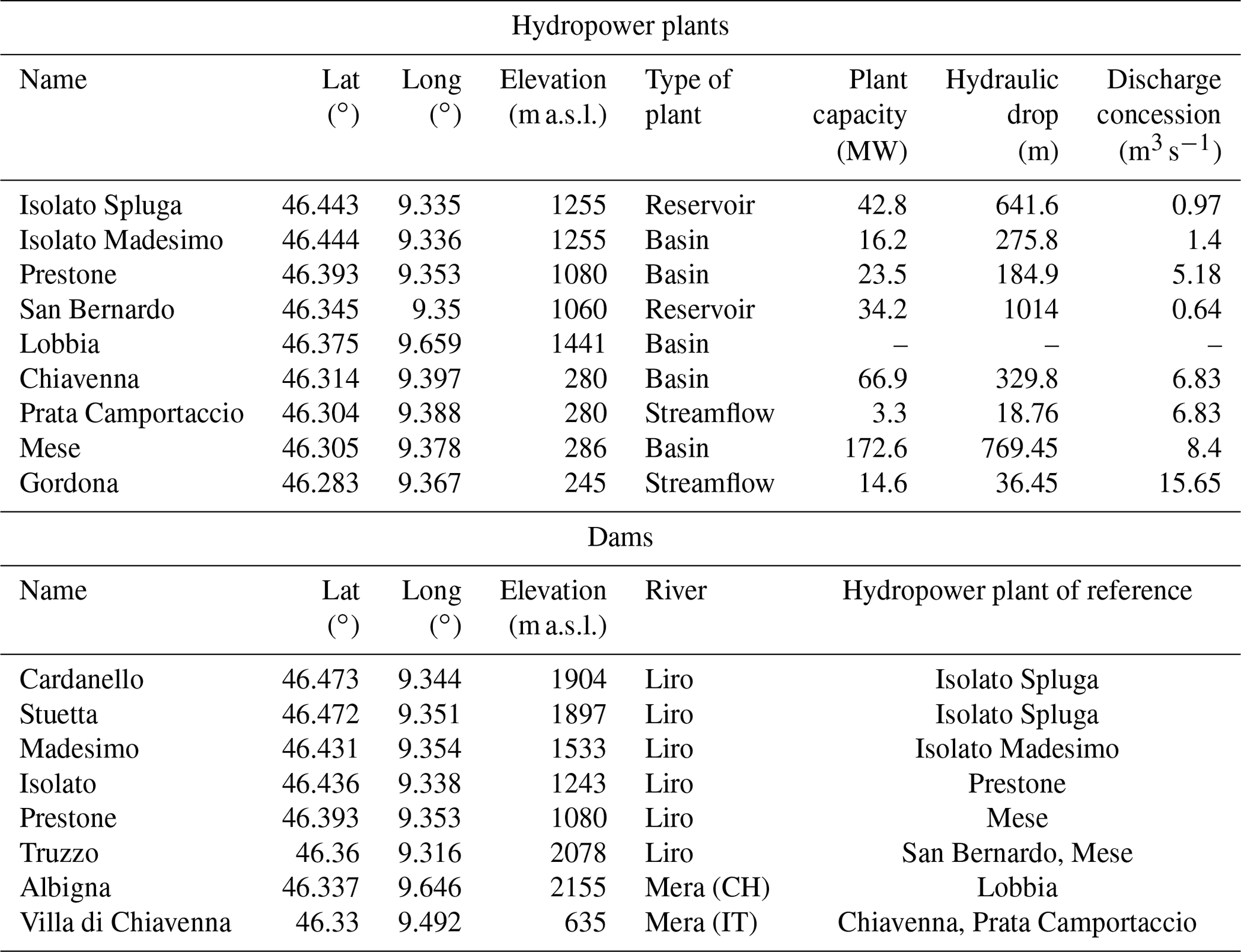
The area is particularly important for hydropower production, and its water resources are largely exploited. Hydropower plants and dams are sketched and described in Fig. 1 and Table 1.
Table 1Description of hydropower plants and dams exploiting Mera water resources. The Liro stream is one of the main tributaries of the Mera River and joins the latter in Prata Camportaccio.
2.2 Dischma
The Dischmabach is a steep, high-Alpine catchment located in the eastern part of the Swiss Alps (Fig. 1). It has two equal source streams whose source areas are the Scaletta Pass and Fuorcla da Grialetsch. Both source streams unite at Dürrboden; the Dischmabach then flows 15 km north-west into the Landwasser in Davos Dorf. The climatological region of the catchment is in the transition zone between the wet northern Alps and the dry central Alps. The aspect is S/SE to N/NW. The catchment's surface is 43.3 km2, including a small glacierized part of 2.1 % of the basin's extension. Elevation ranges from 1668 to 3146 m a.s.l. with a mean altitude of 2378 m a.s.l. In the lowest part, snow accumulates between November and February, whereas in the highest part, the accumulation season ends in April (Zappa et al., 2003).
2.3 Hydrological data
2.3.1 FOEN data
The discharge gauge of Kriegsmatte is the only measuring station within the Dischma catchment. The gauge is located at 1668 m a.s.l. on the right-hand side of the stream. Data monitoring started in 1963. Quality-controlled discharge at hourly resolution is provided by the Swiss Federal Office for the Environment (FOEN, 2018).
2.3.2 Adda Consortium data
Despite its size, discharge data for the Mera catchment are only available at Samolaco, close to Lake Mezzola, in one of the final sections of the river. Discharge data are available from the Adda Consortium (Adda Consortium, 2022) for a fee. The consortium provides the hydrometric level and the rating curve from which discharge is evaluated. Data are available at semi-hourly scale and eventually aggregated at daily scale. Discharge modelling here may be slightly disturbed by hydropower regulation: specifically, there is a shift in volume at the hourly scale on working days (Monday to Friday). However, at the daily scale and at longer timescales, streamflows are not largely disturbed overall, and hydrological modelling exercise provides acceptable results (Fuso et al., 2021). Unfortunately, due to their difficult availability, there is no specific information on water use by plants of the Valchiavenna.
2.3.3 River regulation over the Mera catchment
As mentioned in Sect. 2.1, this area is exploited quite intensely by a complex system of reservoirs and hydroelectric power stations (Table 1). As a consequence, discharge modelling here may be disturbed due to regulation: specifically, there is a shift in volumes at the hourly scale on working days (Monday to Friday). The problem of regulation data availability over the Valchiavenna has already been addressed directly or indirectly in the literature (Fuso et al., 2021; Giudici et al., 2021; Maruffi et al., 2022). In the work of Giudici et al. (2021), dams and plants of the Valchiavenna are simply not considered. In the work of Fuso et al. (2021), the authors underline overall agreement between observed and modelled discharge at the monthly scale, which deteriorates at the daily scale as a result of regulation. The Climate Lab of the Politecnico di Milano has made several attempts at trying to model reservoir operations in the Valchiavenna, but given the impossibility of verifying the assumptions made about reservoir management, the results have never been published. Given these points, and considering the main obstacle of the lack of data in this respect, we decided to neglect the influence of reservoir operation on discharge modelling in the Mera River.
2.4 Meteorological data
2.4.1 MeteoSwiss stations
Meteorological data over Switzerland are partly acquired from the MeteoSwiss (MCH) automatic monitoring network (IDAWEB, 2019). Since no MCH station is installed within the Dischma catchment itself, the nearby stations of Davos (DAV) and Weissfluhjoch (WFJ) provide daily values for air temperature (TA), precipitation (PSUM), wind velocity (VW), relative humidity (RH), and incoming shortwave solar radiation (ISWR). The same variables, except for PSUM, are used for the Swiss side of the Mera catchment from the Samedan (SAM) station in the Upper Engadine.
2.4.2 Intercantonal Measurement and Information System (IMIS) stations
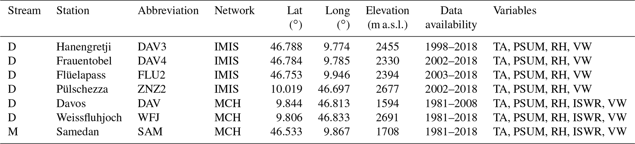
The second part of the meteorological data used for Switzerland comes from the IMIS station network (IMIS, 2019), operated by the WSL Institute for Snow and Avalanche Research (SLF). The IMIS station network does not provide ISWR measurements. Additionally, IMIS rain gauges are not heated, and therefore winter precipitation is obtained indirectly based on snow depth variations and snow settling computed by the SNOWPACK model (Lehning et al., 1999). The information used in this study comes from the IMIS stations located in Davos (DAV), the Flüela Pass (FLU), and Zernez (ZNZ) (see Fig. 1). All data coming from Swiss stations (IMIS, MCH) are presented in Table 2.
Table 2Details about Swiss meteorological stations (IMIS and MCH). The first column of the table indicates the associated river (D and M for Dischma and Mera, respectively). In contrast to ARPA in Table 3, all variables started to be recorded automatically in the same year: 1981.
2.4.3 ARPA Lombardia stations
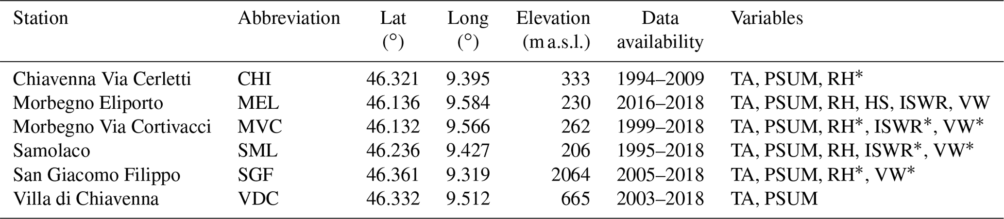
The first automatic meteorological stations were installed in the Italian region of Lombardy only in the late 1980s. Thus, Lombardy can only count on observational time series which, at most, date back to those years. Nowadays, ARPA counts on a network of 318 meteorological stations, but the vast majority of them were only installed in the last 2 decades. As a consequence, there are only few and sparse robust observational time series of the past 30 years in the Valchiavenna. Moreover, historical time series often contain a large number of missing data due to interruption. The stations used in this work are presented in Table 3, and locations are shown in Fig. 1.
Table 3Details about Italian meteorological stations (ARPA). The * symbol next to some of the available variables indicates that such variables started to be recorded later than the first recorded year for TA and PSUM.
2.5 Climate change data
2.5.1 CH2018 data
The climate change section of this paper relies upon the CH2018 climate change scenarios (MeteoSwiss, 2018). These scenarios were derived from the new EURO-CORDEX ensemble of climate simulations with regional climate models (RCMs) (Jacob et al., 2014; Kotlarski et al., 2014). The RCM simulations of EURO-CORDEX were performed using a common model domain centred on western Europe. RCMs dynamically downscale coarser global projections (from global climate models, GCMs) into a resolution which is more suitable for representing the topography of Switzerland. However, RCM simulations from EURO-CORDEX do provide information at a spatial resolution of 0.11 or 0.44∘, which is still too coarse for local impact assessments and might lead to biases, especially for complex orographies. CH2018 applied quantile mapping for spatial downscaling to both observations at station scale and gridded observations at 2 km to derive site-specific projections. Thus, CH2018 can provide projections at daily resolution for the MCH automatic weather station network. Available variables are the mean, minimum and maximum near-surface air temperature, relative humidity, wind speed, cumulative precipitation and incoming shortwave radiation; 68 model chain outputs are provided under three representative concentration pathways: RCP8.5, RCP4.5 and RCP2.6. In this paper, we considered a selected subset of 17 out of the original ensemble, summarized in Table 4. This subset of model chains has already been used in previous studies (Epting et al., 2021; MeteoSwiss, 2018), and it was chosen because it allows us to capture both high and low climate change signals for air temperature and precipitation, limiting the computational demand at the same time.
Table 4Details about the considered climate models. GCM: global climate model. RCM: regional climate model. RCP: representative concentration pathway.

2.5.2 Quantile mapping on MCH, IMIS and ARPA data
The availability of CH2018 downscaled scenarios is restricted to the MCH station network. We adopt the methodology presented by Rajczak et al. (2016) and apply it to IMIS stations (Michel et al., 2021). This quantile mapping (QM) methodology enables the spatial transfer of the future climate projections from the set of CH2018 MCH stations to a different network. We extend the dataset from Michel et al. (2021) to the ARPA network to have consistent climate change projections for all our stations.
The procedure is summarized in the following: as a first step, the so-called most representative station (MRS) is selected from the MCH CH2018 network for each ARPA station. The MRS is selected by maximizing a combined correlation score between observed mean daily temperature and cumulative daily precipitation time series. The combined correlation score is computed over a time span which depends on the first available observations within the ARPA network (see Table 3). Climate scenarios are bias-corrected to match the long-term observational MCH CH2018 time series and, as a second step, they are spatially transferred from the selected MRS to the sparsely observed site within the ARPA network. For further details on this method, we refer readers to Rajczak et al. (2016). On the one hand, Rajczak et al. (2016) performed a robust validation of this method using long-term, multi-variate measurements, revealing satisfactory performance even in topographically complex terrains. On the other hand, limitations for the application of the method remain and concern different aspects besides the well-known uncertainties related to climate projections themselves (Hawkins and Sutton, 2009, 2011). The main untailed uncertainties can be related to (1) possible non-stationarities of transfer functions under climate change (Christensen et al., 2008; Boberg and Christensen, 2012; Maraun, 2012; Bellprat et al., 2013), (2) the fact that climate change signals are imposed by the location of the MRS, and (3) the fact that the spatial transfer also bears uncertainties, especially for spatially and temporally heterogeneous variables such as precipitation. Nonetheless, this method was specifically tailored to improve climate projections for sites affected by data scarcity, also addressing the fact that the closest station is not necessarily the most representative for the observed one. The QM spatial transfer is thus applied to the ensemble of ARPA stations, resulting in climate projections spanning to the end of the century.
Climate change simulations presented in Sect. 4.2.4 are run for the hydrological years 1991–2000 and 2081–2090. We will refer to the first decade as the “reference period” and to the last one as the “climate change period”. For simplicity, we use full decade names further in the paper (e.g. 1990–2000 for the hydrological decade 1991–2000, meaning October 1990 to September 2000).
2.5.3 Temporal downscaling
CH2018 scenarios for Switzerland only provide data at daily resolution. However, such temporal resolution can be too coarse for these data to be used as input to physically based models such as Alpine3D and StreamFlow. This paper follows the method recently proposed by Michel et al. (2021), which provides hourly downscaled climate change time series for MCH and IMIS stations. The same approach was used to obtain hourly climate projections for ARPA stations by first disaggregating the MRS time series (according to the approach by Rajczak et al., 2016, described in the previous Sect. 2.5.2) and then applying the trend to ARPA stations. This approach is based on the delta-change method, which was also used in the previous CH2011 scenario (MeteoSwiss, 2011). In Michel et al. (2021), this procedure is further developed, especially in the sense of the quality assessment of the generated time series and the validation of the parameters. This enhanced method highlights that the original approach used in CH2011 did not represent correctly the seasonal cycle of the climate change scenarios. Furthermore, the method originally developed was validated only for temperature and precipitation, whereas the new method is validated on the five variables that are used in this paper. Time periods of 10 years are used (using the period 2005–2015 for a historical baseline). The work of Michel et al. (2022) shows that using 10-year time periods for applications such as in this study leads to similar results to using 30-year periods. This finding is highly relevant for this paper for a twofold reason. On the one hand, this allows us to include data from IMIS stations. Although IMIS data are not available over the last 30 years to well represent climatic cycles, the 10 years available have proven to improve discharge simulations over Alpine areas (Schlögl et al., 2016). On the other hand, without this finding, no climate change study would be possible within poorly gauged catchments whose surveying does not date 30 years back, such as Mera.
2.6 Geographical data
2.6.1 Digital elevation model (DEM) and land use
On the Swiss side, the DEM used is the DTM25 dataset at 25 m resolution provided by Swisstopo, which is then resampled to the desired resolution of 500 m. Land cover data are derived from the 2006 version of the Copernicus Corine Land Cover (European Environment Agency, 2013) dataset at 100 m resolution and then upscaled to 500 m. Corine Land Cover classes are translated into the land cover classes available in A3D, listed in Michel et al. (2021). On the Italian side, the DEM is provided by NASA (https://earthdata.nasa.gov/, last access: 27 March 2021) and land cover data by CLC. The initial resolution of the DEM is 30 m and is then upscaled to 500 m.
For the Alpine3D model over the Dischma catchment, the computational resolution was chosen, referring to the work of Schlögl et al. (2016). In this paper, the authors test the effects of Alpine3D input variation on snow water equivalent (SWE) quantification, and a big effort is spent on testing different horizontal DEM resolutions. The authors selected four different resolutions (25, 200, 500, 1000 m) for the DEM grid and land cover data. Results show that, downscaling from a horizontal resolution of 500 m to one of 25 m, the relative difference in SWE decreases by only 3 % approximately. Considering such findings, we decided that this simplification would have been acceptable for the scopes of our paper. Besides, the focus of our paper is finally the estimation of the discharge and the benefits of a slightly more accurate SWE quantification risk being lost in the flow-routing process – especially during the calibration. In addition, A3D being a complex model, a 100 m resolution over the ∼5 times larger Mera catchment, i.e. a computational cost multiplied by 25, is technically not doable. For consistency, a resolution of 500 m was kept in Poli-Hydro as well. Given that we had no previous similar sensitivity studies over Mera, we tried an alternative calibration therein with a resolution of 100 m using the Poli-Hydro model. This has not led to significant improvements in performance scores in the face of considerably higher computational times. Therefore, the use of a 500 m resolution was justified over Mera as well.
For the StreamFlow flow-routing model (see Sect. 3.1.2), watershed, sub-watershed and stream network are derived using the TauDEM software (Tarboton, 1997) coupled with a wrapper (Michel et al., 2022) to force it to reproduce exactly the stream network provided by the FOEN (Swiss Federal Office for the Environment, 2020).
Conversely, the Poli-Hydro model simulates the hydrological balance and the flow routing for the catchment area (through flow directions and flow accumulations), which is identified from the DEM using ArcGIS software (ESRI, 2012). The DEM used was previously upscaled to match the chosen resolution of 500 m.
It is important to underline here that the two approaches prepare the DEM in different ways, thus justifying slight differences in basin shape hereafter.
2.6.2 Glacier data
For both catchments, we use glacier height maps from Zekollari et al. (2019). By means of an innovative model called GloGEMflow, the authors have developed the first regional Alpine glacier modelling making use of high-resolution climate model outputs from EURO-CORDEX (Jacob et al., 2014; Kotlarski et al., 2014). Glacier height needs to be understood as the ice depth above a bottom surface. Such maps are used as an initial condition of each past and future (climate change) simulation. For historical periods, all calibrations are run with the 2005 glacier map as the initial condition. Glacier evolution is then treated and simulated according to the two models and melt schemes. A due consideration is that glacier maps do overwrite the CLC land cover classes, and in the case that a pixel is classified as a glacier by CLC but not by Zekollari et al. (2019), that pixel is simply converted into bare rock.
3.1 Model description
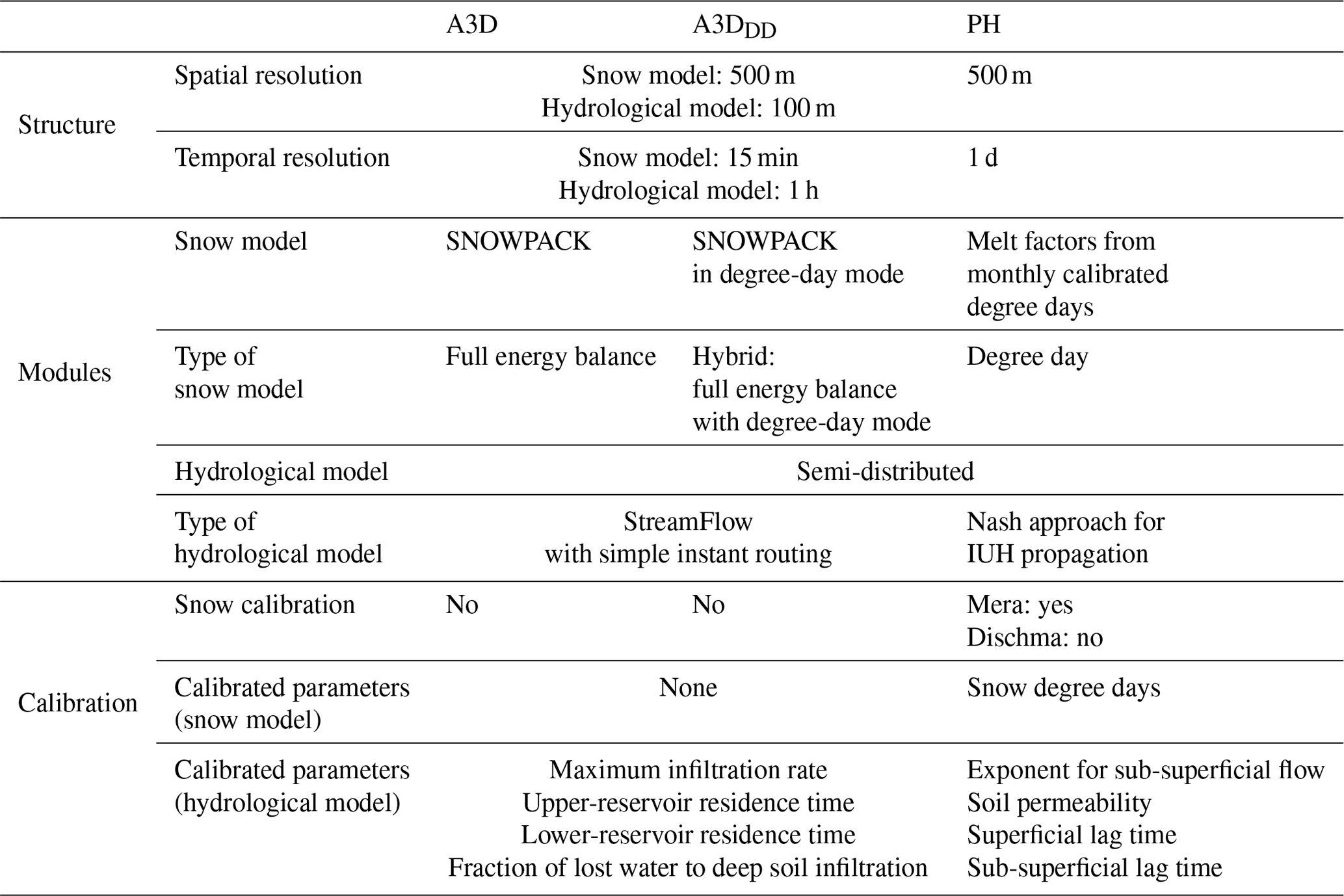
In this study, two different models are compared: the process-based Alpine3D + StreamFlow model chain in its full energy-balance solver and in a hybrid degree-day version (A3D + SF and A3DDD + SF, respectively, hereafter) and the Poli-Hydro degree-day model (PH hereafter). Interestingly, both models have been used recently to perform climate change studies. In Michel et al. (2022), the A3D + SF chain is used to investigate future water temperature of Swiss rivers under climate change. Fuso et al. (2021) used PH to evaluate future hydrological scenarios for the Lake Como catchment in Italy according to three GCMs of the Sixth Assessment Report (AR6) of the IPCC driven by four shared-socio-economic-pathway-based scenarios. A3D is first run in order to obtain the soil runoff, and in a second step SF is run for the hydrological routing using A3D output as input. PH solves within the same model the surface mass and energy balance in order to obtain soil runoff and the hydrological routing. All the models rely on a semi-distributed routing model. The use of a semi-distributed modelling approach rather than a fully distributed one can be justified by the following reasons. In the first place, the increase in spatial resolution introduces two well-known problems: overparametrization and equifinality (Beven, 1989, 1993, 2006). More complexity in spatial detail results in more parameters being involved and, therefore, potential issues in calibration, such as equifinality. Secondly, computational times are consistently higher for fully distributed models. For these reasons, semi-distributed or purely conceptual models are preferred in most studies, justifying our choice to rather assess those kinds of models. Overall model differences (structure, modules, calibrated parameters) are summarized in Table 5. The models are then introduced separately in Sect. 3.1.1 and 3.1.3.
Table 5Summary of the main features and differences of the models used for the case studies.
The forcing meteorological data at the station location are extrapolated to the grids in A3D using a distance-weighted method with vertical lapse rate corrections (see details in Michel et al., 2022). Longwave radiation is also computed in A3D using TA, RH and cloud cover derived from ISWR using the approach described in Omstedt (1990). The gridded data are written out and also used in PH in order to use exactly the same forcing data. The grids are produced at a 500 m resolution to match the topographical resolution.
3.1.1 Alpine3D
The Alpine3D model (Lehning et al., 2006) is a deterministic and spatially distributed model designed for high-resolution simulation of snow processes in topographically complex areas. In A3D, the SNOWPACK model (Lehning et al., 2002) is applied to each cell of the catchment (here a 500×500 m grid). SNOWPACK is a physical 1-D multi-layer snow and soil model formerly developed for avalanche warning. It comes with a detailed description of the snow micro-structure, and it resolves phase changes in snow on a physical basis. SNOWPACK also contains a two-layer canopy module simulating the micro-meteorology in the forest, the evapotranspiration and the interaction between trees and snow, including snow interception (Gouttevin et al., 2015). Within A3D, the SNOWPACK model is run for every cell of the catchment at a 15 min time step, while the forcing boundary conditions are updated on an hourly basis. A3D also has a radiative sub-module enabling the consideration of topographic shading, terrain reflection and atmospheric cloudiness on shortwave radiation distribution. Topographic effects deeply influence radiation balance in mountain regions. In fact, the intensity of incoming and outgoing radiative fluxes depends on many factors, such as surface inclination angle, shading and surface properties (von Rütte et al., 2021). In mountain terrain, incoming longwave radiation decreases with elevation because higher areas have an enhanced angular exposure to the radiating sky, which is colder than the terrain (Lehning et al., 2006). A3D is run with the same set-up described in detail in Michel et al. (2022), to which we refer the reader for further details.
A3D can also be run in a hybrid simpler melt-factor energy-balance mode (Shakoor et al., 2018). This set-up is called A3DDD. In A3DDD, the melt rate is linearly linked to air temperature by the temperature melt factor (TMF). In A3D, A3DDD can be used within SNOWPACK as an energy boundary condition at the snow–atmosphere interface. When a melt phase occurs, i.e. when water and ice are coexisting in the snow element and air temperature is larger than snow surface temperature, the energy entering the snowpack is computed with A3DDD. Radiative fluxes are set to zero in the uppermost snow element and the turbulent fluxes are not computed anymore. When the snowpack is not in a melting phase, the net energy flux at the snow surface is computed by solving the standard energy-balance boundary condition (Schlögl et al., 2016). Ice and snow are not distinguished by the A3DDD melt model: a single TMF value is used for both of them, although such an approach has been shown to be oversimplified for glacierized catchments (Hock, 1999). The energy balance (EB) in case of melting is computed by A3DDD as in Eq. (1).
In Eq. (1), TMF is the temperature melt factor; Tair and Tsnow are the air temperature and snow temperature, respectively.
3.1.2 StreamFlow
StreamFlow is a semi-distributed hydrological model described in Gallice et al. (2016). The runoff output produced in A3D is collected into each sub-watershed in SF, and the residence time in the soil is determined with an approach using two linear reservoirs. The water is then routed to the river. While SF offers multiple routing schemes, the simple instant routing scheme shows a similar performance to more complicated ones for Alpine catchment studies (Michel et al., 2022), and thus we use this scheme in the present work. SF is run at an hourly time step and at a spatial resolution of 100 m. Further details about the set-up used for SF can be found in Michel et al. (2022).
3.1.3 Poli-Hydro
Poli-Hydro is a spatially semi-distributed, cell-based hydrological model suitable for the simulation of high-altitude, poorly gauged catchments (Bocchiola et al., 2018; Casale et al., 2020). It is able to reproduce deposition of snow and ablation of snow and ice through the accumulation of thermal time, i.e. the daily sum of degree days. The model works at a daily timescale, and it is based on the mass conservation equation. The mass balance involves liquid and solid precipitation, snowmelt, glacial ablation, effective evapotranspiration and groundwater discharge. The model takes as input data a DEM, a land cover map and daily values for air temperature and total precipitation. As mentioned before, input data are the meteorological forcing grids extrapolated by A3D. This model conceives the formation of flow by means of two mechanisms: superficial and groundwater discharge.
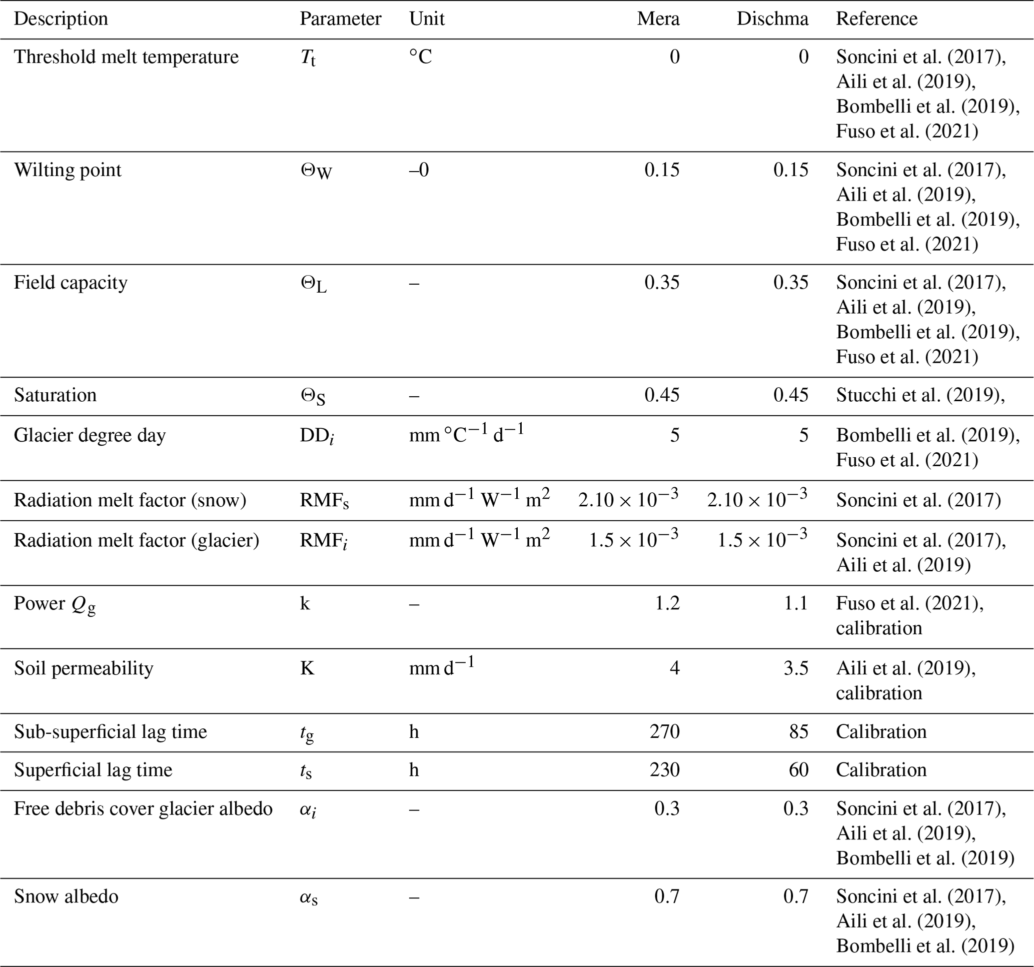
Snowmelt and glacial ablation are estimated by means of a melt factor (Eq. 2). Here, the model takes into consideration contributions from shortwave radiation and temperature (Aili et al., 2019; Bombelli et al., 2019; Stucchi et al., 2019).
In Eq. (2), Ms and Mi are the melt factors for snow and ice, respectively, T the mean daily temperature, DDs and DDi the degree days for snow and ice (Table 8), Tt the threshold temperature equal to 0 ∘C, RMFs and RMFi the radiation melt factors, αs,i the snow and ice albedo (Soncini et al., 2017), and qsw the shortwave radiation flux. Ice melt and snowmelt occur only when the average daily temperature is higher than the threshold temperature. Ice melt occurs on ice-covered domain cells once snowmelt is completed.
Superficial flow Qs is only generated in the condition of saturated soil (Eq. 3).
In Eq. (3), S is the soil water content evaluated from the mass balance equation for each time step and Smax is the greatest potential soil storage calculated by the curve number method (Cronshey, 1986) from a land cover map for each cell of the catchment. The sub-superficial discharge Qg is computed as in Eq. (4).
In Eq. (4), K is the saturated permeability and k is a power exponent.
Then, for the flow routing, two parallel systems are considered, one for superficial flow and one for sub-surface flow. Two instantaneous unit hydrograms u(t) (IUHs) are evaluated for each cell using the Nash approach (Rosso, 1984) for superficial and sub-surface flow, respectively.
3.2 Statistical scores
Statistical scores are used to assess the models' predictive performance. In this work, three metrics are used: the root mean square error (RMSE, Eq. 5) for the snow cover analysis in Sect. 4.2.1, the Nash–Sutcliffe efficiency (NSE, Nash and Sutcliffe, 1970, Eq. 6) and the Kling–Gupta efficiency (KGE, Gupta et al., 2009, Eq. 7) for the comparison of predicted discharge in Sect. 4.2.
With respect to NSE (Eq. 6), the value NSE=0 is commonly regarded as an inherent benchmark for model performance (Schaefli and Gupta, 2007; Knoben et al., 2019), as it describes the situation where the average of the observations has the same explanatory power as the model's predictions.
The KGE score (Eq. 7) further extends NSE into three different components: the correlation r, the flow variability error α and the mean flow bias β. It is important to remark that, as explained in Knoben et al. (2019), it is impossible to define within KGE a benchmark value that acts as a threshold between a “good” and “bad” model. To keep consistency with NSE, here we will consider as a benchmark the case where , which yields (Knoben et al., 2019) and corresponds to NSE=0. The need to consider the KGE in addition to the widely used NSE mostly arises from two important drawbacks of the NSE. In the first place, the use of the observed annual mean as a benchmark can be a mediocre predictor (Schaefli and Gupta, 2007), especially for strongly seasonal discharge time series such as those dominated by snowmelt, leading to the overestimation of the model efficiency. Secondly, the NSE computes squared differences between the observed and predicted values. As a result, the metric becomes excessively sensitive to extreme values by enhancing higher-magnitude streamflows and neglecting lower ones (Legates and McCabe, 1999; Criss and Winston, 2008). It is important to note that PH is calibrated using the NSE metric as the score to maximize, while SF uses the KGE metric, so each model might be biased toward better performance in its respective calibration metric.
4.1 Calibration
4.1.1 Alpine3D
As mentioned in the Introduction, A3D is used “as is” and does not need to be calibrated in a strict sense. As explained in Michel et al. (2022), a number of runs are normally performed with different values of precipitation vertical lapse rate to match the yearly total mass over the catchments, and where available, modelled snow heights are compared against measurements to assess the model's capacity to reproduce snow season dynamics in terms of its duration. Therefore, although some parameters are effectively adjusted, no real calibration is performed within A3D.
4.1.2 StreamFlow
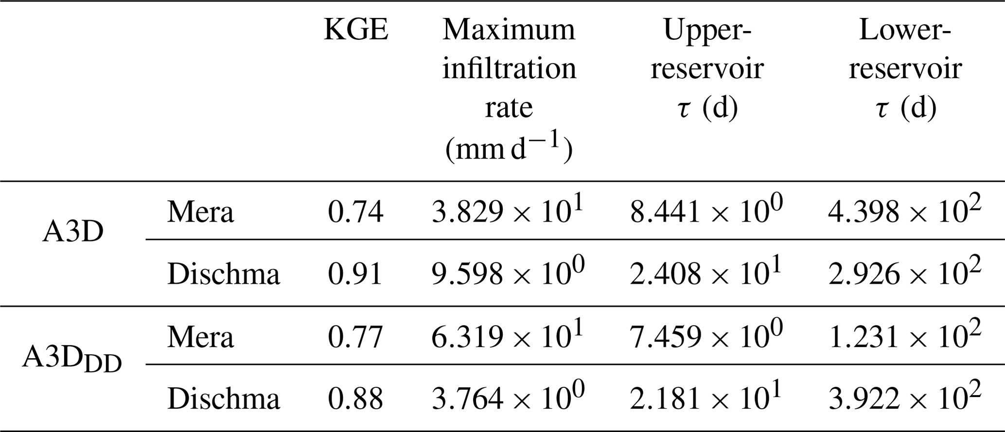
To calibrate the model SF, 10 000 calibration runs are performed over the calibration period October 2010 to September 2014 (the validation period being from October 2014 to September 2018). The following parameters are calibrated: maximum infiltration rate, upper-reservoir residence time (τ), lower-reservoir τ and fraction of water lost to deep soil infiltration. The calibration is achieved with a Monte Carlo approach using 10 000 random parameter sets and the corresponding model runs over the historical period. The random sets are drawn from uniform distributions, with bounds corresponding to standard values available in the literature (see Gallice et al., 2016). The performance is assessed using the KGE. SF is calibrated separately for the run with A3D in full energy-balance mode and for the run with A3DDD.
For the Mera catchment, a KGE value of 0.74 is obtained for the calibration period (0.77 with A3DDD). For the Dischma catchment, a value of KGE=0.91 is obtained (0.88 with A3DDD). The values of the parameters obtained are given in Table 6.
4.1.3 Poli-Hydro
Snowmelt calibration
In PH, degree days for snowmelt are calibrated using a two-step method. First, the simulated snow cover area (SCA) is compared against MODIS satellite images (snow cover extent, Copernicus Global Land Service, available online: https://land.copernicus.eu/global/products/sce, last access: 30 March 2021). Such validation is performed once every 15 d, i.e. the overpassing frequency of the MODIS satellite in the area of the Valchiavenna. This method gives information about the SCA extension, although it is not possible to verify snow depth. To cover this, snow depth data measured at AWS are collected. For the Mera catchment, snow depth data for the entire simulation period are only available at the San Giacomo Filippo station (SGF, lat 46.361∘, long 9.319∘; 2064 m a.s.l.). Monthly values of snow degree days are reported in Table 7. The simulated snow water equivalent is compared with measured snow depth at the AWS. Within the Dischma catchment itself, MCH/IMIS snow depth data are not available; therefore, only SCA is verified. Detailed approach and results are reported for the Mera catchment in Fuso et al. (2021). The validation of the modelled snow dynamics is performed by comparing observed and modelled time series of snow depth. To this aim, the daily modelled snow water equivalent is converted to snow depth using the approach proposed by Martinec and Rango (1989) and more recently implemented in Aili et al. (2019). It is important to remark that the approach by Martinec and Rango (1989) is only used to verify the modelled snow water equivalent against the measured snow depth. The PH model does not model physical processes and energy fluxes within the snowpack layers. For additional details on this procedure, we refer to the aforementioned papers.
Table 7Snow degree days used by the Poli-Hydro model for the Mera and Dischma catchments.

Flow-routing calibration
For the flow propagation, PH is then fed with a set of fixed calibration parameters from other previous studies on the same areas of the central Alps and Valtellina (Soncini et al., 2017; Aili et al., 2019; Fuso et al., 2021). To feed the model with plausible parameters verified in previous studies is a common practice in operational hydrology to ease the multi-objective optimization problem. Moreover, many such fixed parameters are physically based and refer to the soil type, land cover and other “static” properties of the area, which are unlikely to change in the short term. The following parameters are calibrated: soil permeability, saturated permeability K, power exponent k and lag times (superficial ts and sub-superficial tg). The initial values of K and k are taken based on literature research on the study area (Aili et al., 2019) and then (manually) iteratively tuned by fitting modelled discharge against observed discharge. Lag times are assessed according to power law functions of the basins' contributing area for both superficial and sub-superficial flow (Casale et al., 2020). Model parameters are listed with references in Table 8 for the Mera and Dischma catchments. Calibration is performed from October 2010 to September 2014 and validation from October 2015 to September 2018. For model calibration and validation, simulated discharge at each catchment's closure section is compared with the observed value. The percentage bias (PBIAS) and the NSE are computed during the calibration: the absolute value of the PB is minimized and the NSE is maximized. Results are reported in Table 9.
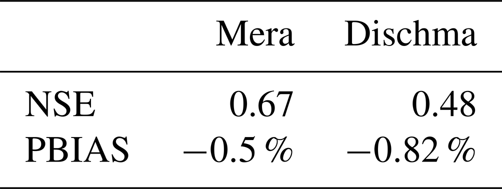
We are aware that the calibration score obtained over the Dischma catchment is not ideal, even though it is still considerably higher than zero, thus holding more explanatory power than the time series mean. The explanation we give to this score is twofold. On the one hand, there is the spatial resolution of the computations. In Sect. 2.6.1, several reasons have been listed why a resolution of 500 m might be the best compromise for this case study. Such a resolution, which may be functional for full energy-balance schemes and/or large catchments, may prove to be not optimal for degree-day schemes applied to catchments like Dischma. Indeed, as explained in Sect. 2.2, Dischma is a small and steep catchment with a very significant altitude range. It could be the case that, in contrast to what might happen in a larger and less topographically complex basin like Mera, over the same domain cell the elevation difference could vary a lot. To flatten this difference implies flattening temperature variation and thus snowmelt dynamics within a scheme (i.e. the degree day) that already flattens temperature variations within the same day. On the other hand, unlike in the case of Mera, due to the lack of MCH/IMIS snow height measurements within the basin, snow is not calibrated over Dischma by the PH model. All hydrological parameters are therefore calibrated with a single objective function (i.e. the measured discharge), so achieving convergence becomes more complex, resulting in poorer performance scores. However, we believe that the resolution of 500 m is still adequate for our case study, and despite these drawbacks in the specific case of Dischma, we believe that it does not invalidate the general findings of our work.
4.2 Model comparison
As mentioned in the Introduction, the use of degree-day models might be preferred for the lighter computational load and the lowest number of input data required, but on the other hand, their use for climate change impact studies is disputable. With the aim of performing climate change impact studies, the objective is to assess the models' efficiency in reproducing discharge and total volumes at the river section of interest. However, high-performance discharge simulations strongly depend on the correct representation of runoff formation. Specifically, runoff in Alpine catchments can be separated into two main components: fast runoff, which is mainly due to precipitation and surface flow, and slow runoff, generated by snowmelt and ice melt and sub-surface flow. In this section we compare the models presented in Sect. 3.1.1–3.1.3 in three different ways: (1) by means of a snow cover analysis, (2) before flow routing (referring to the water volume released at each pixel of the catchment domain) considering the different contributions to the total runoff (precipitation, snowmelt and glacier melt) and (3) after flow routing (referring to discharge and volumes). When discussing runoff contributions, before flow routing, we refer to the models as A3D, A3DDD and PH, respectively, for Alpine3D (in its full solver and hybrid degree-day version) and Poli-Hydro (Sect. 3.1.1 and 3.1.3). Conversely, for discharge and volumes, after flow routing, we refer to the same models as A3D + SF, A3DDD + SF and PH + PHR, respectively, for streamflow (forced with A3D and A3DDD) and the flow-routing scheme of PH (Sect. 3.1.2 and the flow-routing scheme in Sect. 3.1.3).
4.2.1 Snow cover analysis
In the first place, the models are implemented with different temperature thresholds for rain–snow separation, 0 ∘C for PH (Fuso et al., 2021) and 1.5 ∘C for A3D and A3DDD (Michel et al., 2022), as this is the way they are typically used. As a result, PH may simulate more liquid precipitation than A3D in winter which does not accumulate as snow (see Fig. 2).

Figure 2Comparison of solid and liquid precipitation in A3D/A3DDD and PH for the Mera (a) and Dischma (b) catchments.
Figure 3 shows observed and modelled snow height and snow water equivalent within the Mera domain in the cell where the high-elevation station of San Giacomo Filippo is located. Snow water equivalent (i.e. snow density) measurements are not available for this station. A similar analysis was not possible for Dischma, because the MCH/IMIS dataset used for this paper did not contain snow depth or snow water equivalent measurements within the basin itself. Model performance in reproducing snow height is rated by means of RMSE. Snow height is best reproduced by A3D, which gives the lowest RMSE (top right of Fig. 3a). A3DDD tends to underestimate snow height; however, RMSE is only slightly higher than A3D. PH shows the highest RMSE. Common errors for A3D seem to be related to compaction, for A3DDD to an excessively fast melting, whereas PH shows errors in accumulation and melting. The poorer performance of PH may be explained by the relative simplicity of the assessment of snow depth from snow water equivalent by means of the approach from Martinec and Rango (1991) mentioned in Sect. 4.1.3. PH systematically simulates a lower snow water equivalent than A3D. Exceptions are the years 2010 and 2014, when snow water equivalent predicted by A3DDD is more in agreement with PH rather than A3D. Despite measured snow water equivalent not being available here, the literature generally agrees on A3D often outperforming simpler models in reproducing it, for example in Terzago et al. (2020). With reference to Sect. 4.1.3, it is important to remark that the station of San Giacomo Filippo is used to calibrate/validate snow water equivalent in the PH model but not in A3D/A3DDD. On the one hand, the comparison is uneven, but on the other hand it is relevant that A3D and A3DDD outperform PH there.
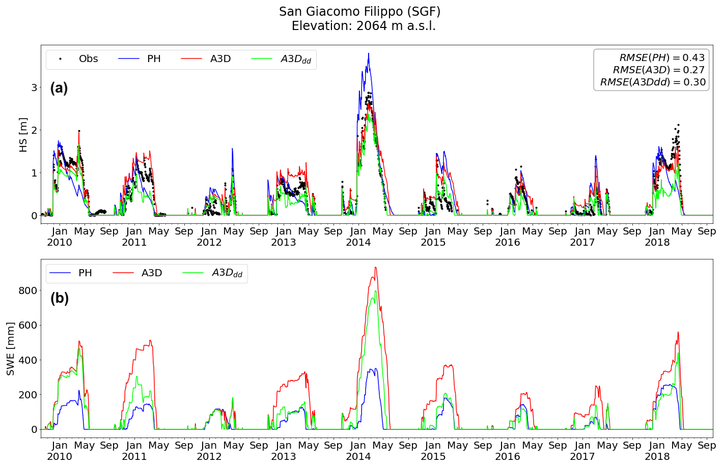
Figure 3Snow cover analysis for the high-altitude station of San Giacomo Filippo within the Mera catchment. Panel (a) shows observed and modelled HS, and panel (b) shows modelled SWE.
Modelled snow water equivalent at basin scale is shown in Figs. 4 and 5. As already observed in Fig. 3, A3D reproduces systematically higher snow water equivalent compared with A3DDD and PH. Snow water equivalent peaks are equally reproduced by all models in terms of seasonality. However, regardless of the catchment and year, PH shows a longer melting season. The reason might be a protracted snowmelt process due to PH's degree-day scheme and the resolution of meteorological forcing: as mentioned in Sect. 3.1.3, the melting scheme only takes into account a mean daily temperature value, which needs to be higher than the melting threshold for any snowmelt to be represented. This condition is likely to be met only after melting has already set in reality, delaying the process of snow ablation and leading to more snow mass predicted for summer months. These findings are confirmed by the work of Terzago et al. (2020), where melt models of lower complexity did show higher biases against observations with respect to more complex ones like SNOWPACK. In Terzago et al. (2020), high biases for simpler models are related both to their underestimation of snow water equivalent peak values and to the protraction of the snowmelt season that they reproduce. Maps of summer months in Figs. 4 and 5 corroborate that PH reproduces a higher snow water equivalent in high-elevation areas, especially in early summer.
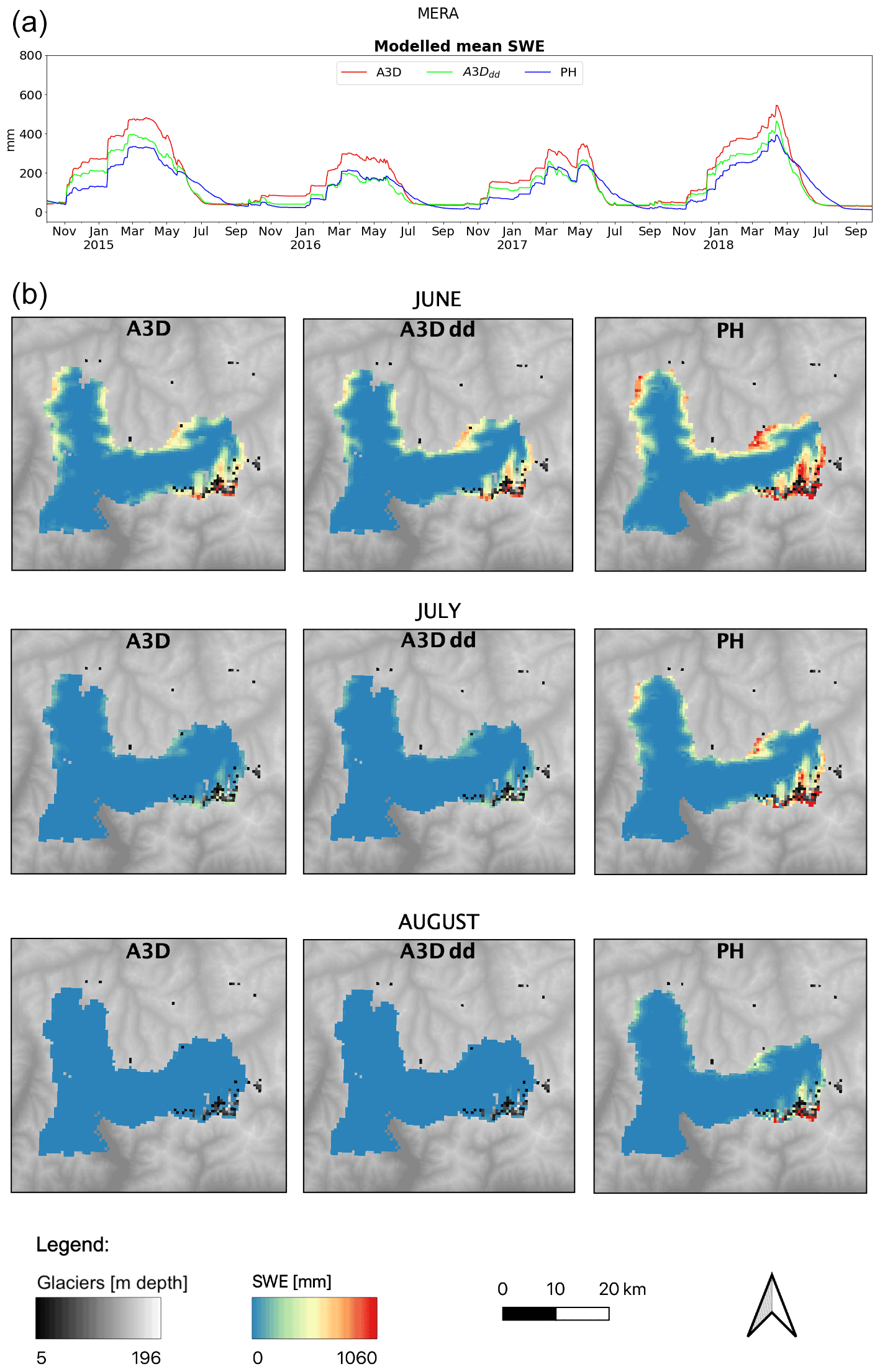
Figure 4(a) Modelled mean SWE over the Mera basin for the validation period. (b) SWE maps for summer months over the Mera basin for the calibration and validation periods.

Figure 5(a) Modelled mean SWE over the Dischma basin for the validation period. (b) SWE maps for summer months over the Mera basin for the calibration and validation periods.

Figure 6Panels (a–c): modelled runoff components over the Mera catchment reproduced with the full solver of Alpine3D (A3D), the degree-day melting scheme of Alpine3D (A3DDD) and Poli-Hydro (PH), respectively. Panels (d, e): discharge and monthly volumes modelled by StreamFlow using output from the full solver of Alpine3D (SF) or its degree-day scheme (SFDD) and modelled by Poli-Hydro (PHR) compared with measurements. Results for the validation years 2015–2018, averaged by day of the year and by month.
4.2.2 Runoff formation
The different components of runoff are shown in Figs. 6 and 7. Throughout Sect. 4.2.1, we underlined major differences among models in terms of snow cover. Such differences lead to discrepancies in modelled snowmelt. As a consequence of the model's structure described in Sects. 3.1.3 and 4.2.1, PH reproduces a delayed and reduced melt season compared with both versions of A3D. Interestingly, A3DDD reproduces a melt season closer to the one obtained with the full solver and more important melt events during the winter.
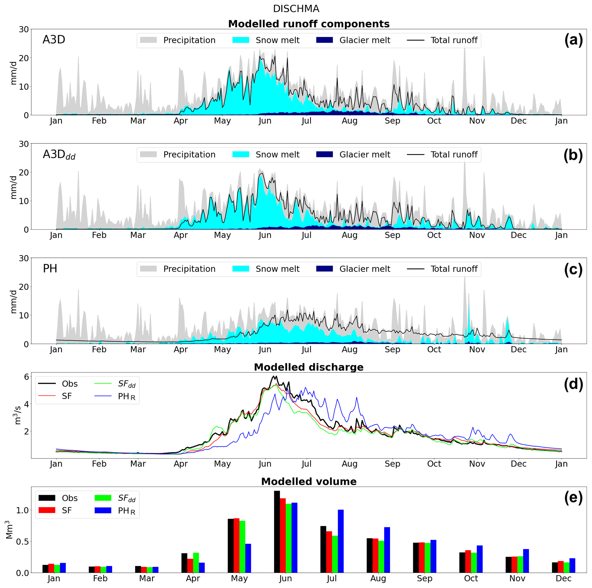
Figure 7Panels (a–c): modelled runoff components over the Dischma catchment reproduced with the full solver of Alpine3D (A3D), the degree-day melting scheme of A3DDD and PH, respectively. Panels (d, e): discharge and monthly volumes modelled by StreamFlow using output from the full solver of Alpine3D (SF) or its degree-day scheme (SFDD) and modelled by Poli-Hydro (PHR) compared with measurements. Results for the validation years 2015–2018, averaged by day of the year and by month.
An altered reproduction of snowmelt seasonality affects model performance in reproducing discharge. In Figs. 6 and 7, observed and modelled discharge after flow routing and monthly averaged volumes are shown. For the Mera catchment, the general behaviour of the three models is quite similar, being characterized by an underestimation of the observed discharge over the accumulation season and overestimation over the melting season. Besides a similar general pattern, SF reproduces the observed flow with more accuracy during the melting season (regardless of being forced with A3D in its full-solver or degree-day version), whereas PHR shows a constant bias towards higher discharges. In addition, PHR does not distinguish between snowmelt- or glacier-melt-dominated seasons, as contributions are smoothed and do not show a predominant presence throughout the melting season. The effect of this is a poorer representation of the observed discharge, where peaks are smoothed and discharge is generally overestimated. For the nivo-glacial regime of the Dischma catchment, the difference between the models is even more evident. The different timings of snowmelt have an important impact on predicted discharge: PHR delays the spring snowmelt-induced discharge by 1 month compared with observations, and additionally it fails to represent the accentuated discharge peak forced by snowmelt characterizing nival rivers (Déry et al., 2009). The explanation is twofold: on the one hand, there is the different rain–snow threshold temperature the schemes are normally implemented with. On the other hand, PH is run at a daily resolution, relying on a melting scheme which only considers the daily average temperature, whereas both versions of A3D are run sub-daily. This has repercussions for the melt dynamics, as will be explained later in Sect. 5.1. The consequence is a poor reproduction of discharge regime and volumes throughout the entire melting season, with severe underestimations in early spring and, correspondingly, overestimation in summer and autumn. Conversely, as a consequence of the correct representation of the melt dynamics, both versions of A3D almost equally reproduce discharge and volumes accurately.
4.2.3 Statistical performance of discharge simulations
In this section, performance metrics described in Sect. 3.2 are used to evaluate discharge simulations. After showing that simpler melt schemes provide an altered representation of runoff seasonality in the previous section, such alterations will be quantified here.
Table 10Performance scores over the validation period for discharge in the Mera and Dischma catchments, for StreamFlow forced by the full-solver output of Alpine3D (SF), the degree-day melting scheme of Alpine3D (SFdd) and Poli-Hydro (PHR).
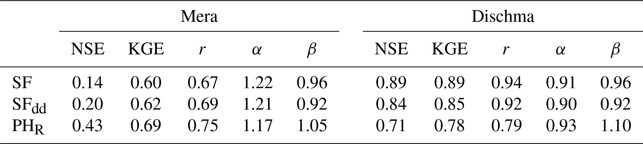
Table 10 shows the models' performance scores over the validation period. In general, better performances are obtained over the Dischma catchment than over Mera, in agreement with what can be seen in Figs. 6 and 7. The Mera River being regulated by multiple dams (Sect. 2.3.3, Fig. 1 and Table 1), this result is not surprising and underlines the issue of not explicitly considering such infrastructures in models. With PHR, better scores are obtained in terms of both annual NSE and KGE over the Mera, although we previously showed that the predicted melt dynamics is substantially wrong, and Fig. 6 shows a clear overestimation of runoff during the summer season. Table 10 also shows the r, α and β components of KGE scores, which express errors in correlation, variability and mean, respectively. Over Mera, PH exhibits a better linear correlation with observed values, a slightly lower variability error and a slightly higher mean error with respect to both versions of A3D. The lower variability error can be explained by the less-accentuated snowmelt-generated discharge, whereas the higher mean error is likely due to the slightly higher baseflow simulated by PH, which may well be induced by calibration. On the other hand, over Dischma, the linear correlation modelled by PH is poorer with respect to both versions of A3D and the mean error is higher, with variability error not changing significantly among models. Errors for correlation and mean are explained by the shifted discharge curve induced by the poorer accuracy of the snowmelt simulation. Both versions of A3D have very similar values of correlation, variability error and bias. All the models predict a higher flow variability with respect to the observed one over the Mera catchment but not over the Dischma catchment, suggesting again the influence of the flow regulation. Over the Dischma catchment, both NSE and KGE show a lower performance of PHR compared with SF, as we can expect since PHR tends to delay the melt season by 1 month. As mentioned earlier, for catchments with strong seasonal signals, using quality metrics on a yearly basis is not optimal. Many authors have addressed this issue by using those metrics on a seasonal basis (Garrick et al., 1978; Martinec and Rango, 1989; Legates and McCabe, 1999; Schaefli and Gupta, 2007). We thus evaluate the models' performances by dividing the validation interval according to seasons. With this approach, the observed discharge is no longer averaged over the ensemble of validation years but rather over the ensemble of validation seasons. As a consequence, the mean flow as a benchmark case gains specific significance as a function of the considered season. The seasonal performance analysis (Fig. 8) shows that, again, lower scores are obtained for the Mera catchment. Overall, both versions of the SF + A3D chain outperform PH + PHR in almost all seasons and in both catchments. PHR obtains remarkably low scores in winter. The delayed melt season of PH for the Dischma catchment is also clearly visible in the scores obtained in the spring season by PHR. Interestingly, both versions of SF + A3D obtain similar scores.
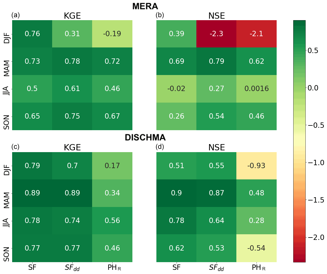
Figure 8Seasonal KGE (a, c) and NSE (b, d) scores obtained over the Mera (top panels) and Dischma (bottom panels) catchments. Scores are shown for the two versions of A3D + SF and for PHR.
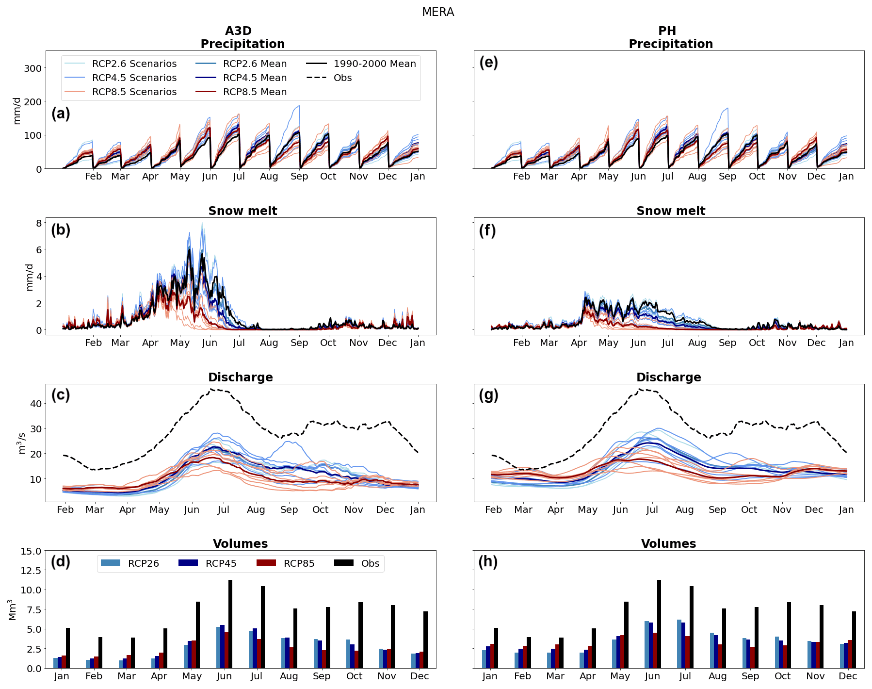
Figure 9Climate change scenarios over the Mera catchment for 2080–2090 against the reference mean over 1990–2000 for precipitation (a), snowmelt (b), discharge (c) and volumes (d) predicted by A3D (a–d) and PH (e–h). Precipitation and volumes are presented as average monthly cumulates. Snowmelt is presented as the average year. Discharge is presented as the average year, smoothed by a moving average with a window of 30 d.
4.2.4 Climate change
Climate change simulations are run over the period 2080–2090 and forced by the set of RCMs listed in Table 4. In the following, we present the predicted evolution of precipitation, snowmelt (as of the most significant seasonal forcing for total runoff and the major difference between the two melt schemes), discharge and total volumes with the aim of discussing the sensitivity of the models to climate change. Glacier melt will not be covered because its influence by 2050–2060 and later is predicted to be extremely small due to glacier retreat. In the following, A3D's degree-day configuration will not be used anymore since, (1) as mentioned before, there are no real computational advantages in using such a scheme with respect to the full solver, and (2) differences with respect to A3D are very small, although they could also increase in a future changed climate. For precipitation and snowmelt, climate change simulations are compared against the mean over the reference period 1990–2000, whereas for discharge and volumes they are compared with the observed time series. The reference period is used here with the only aim of showing seasonality changes induced by climate change, as the models' differences in reproducing melt were already discussed throughout Sect. 4.2.
The predicted evolution of precipitation, snowmelt, discharge and volume patterns is shown in Figs. 9 and 10 for Mera and Dischma, respectively. Boxplots in Figs. 11 and 12 show deviations of the RCP8.5 mean from the mean over the reference period.
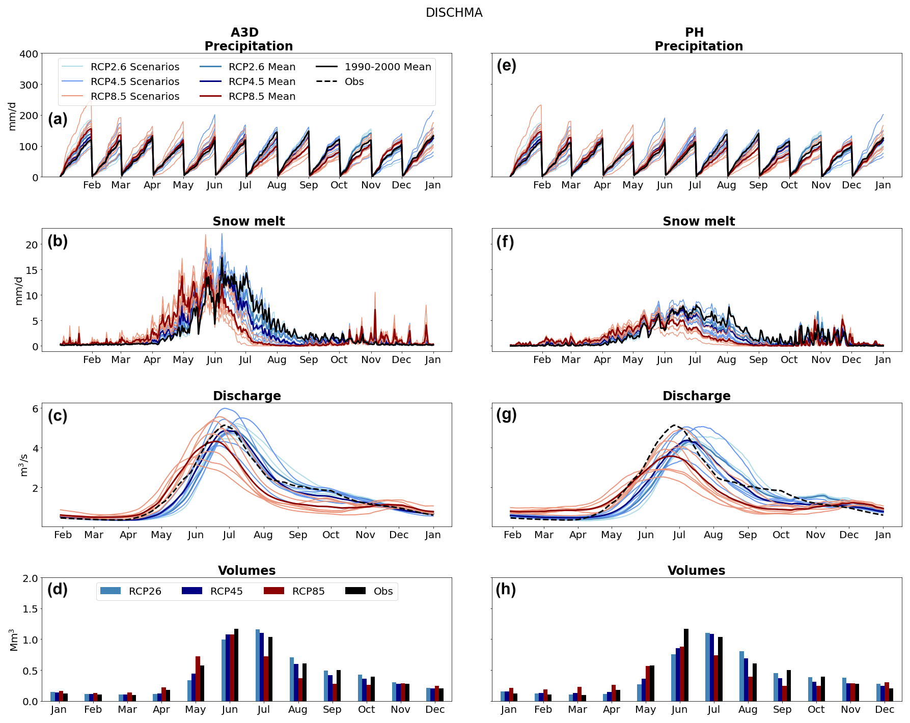
Figure 10Climate change scenarios over the Dischma catchment for 2080–2090 against the reference mean over 1990–2000 for precipitation (a), snowmelt (b), discharge (c) and volumes (d) predicted by A3D (a–d) and PH (e–h). Precipitation and volumes are presented as average monthly cumulates. Snowmelt is presented as the average year. Discharge is presented as the average year, smoothed by a moving average with a window of 30 d.
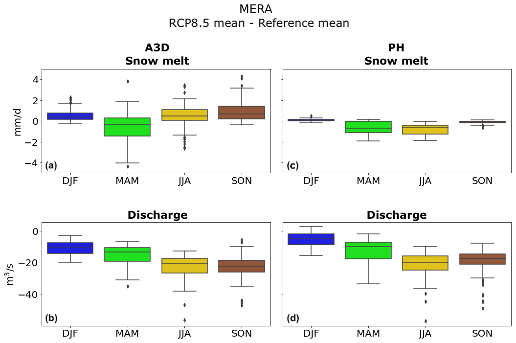
Figure 11Boxplot illustrating the difference between the 2080–2090 RCP8.5 scenario mean and the reference mean (1990–2000) for snowmelt (a) and discharge (b) predicted by A3D (a, b) and PH (c, d) for the Mera catchment.

Figure 12Boxplot illustrating the difference between the 2080–2090 RCP8.5 scenario mean and the reference mean (1990–2000) for snowmelt (a) and discharge (b) predicted by A3D (a, b) and PH (c, d) for the Dischma catchment.
Both models show identical precipitation predictions, thus excluding possible downscaling inconsistencies (Figs. 9a, e and 10a, e).
Changes in snowmelt predicted by A3D and PH are consistent at a seasonal level: with respect to the reference mean over 1990–2000, a net increase is predicted in spring (most evidently in the nivo-glacial Dischma catchment), a net decrease in late summer (August to September) and late autumn (October to November), and an increase during winter months (December to March). Such findings are in line with previous studies, e.g. Bavay et al. (2013) and Kobierska et al. (2013). Although tendencies are similar amongst the two melt models, the magnitude of changes is rather different. The A3D energy-balance model appears to be more sensitive to climate change than the degree-day PH model: not only is the predicted snowmelt significantly higher (up to +50 %), but changes with respect to the reference period are also more marked for both catchments (see Figs. 11b and 12b). Differences in melting magnitude and change are mostly ascribed to spring and summer months. To explain this, the basis of the degree-day melt scheme needs to be discussed again. The main physical processes involved in the energy balance are incoming and outgoing longwave radiation, absorbed shortwave radiation, and turbulent heat fluxes and melt (Ohmura, 2001; Zappa et al., 2003). The degree-day estimation approach of snowmelt/glacial melt of PH relies on air temperature, which is considered to be a good predictor for the majority of energy fluxes taking part in the balance and in absorbed shortwave radiation (see Eq. 2), which is incompletely described by air temperature and whose effect is included through calibrated parameters.
The predicted shift in melting season affects the seasonality of the discharge regime for both catchments. Figures 9c, g and 10c, g show an increase in late autumn and winter discharge for both catchments, which is likely linked to the enhanced snowmelt in late autumn months. Such findings are in line with previous studies about climate change in mountain catchments, e.g. Michel et al. (2022). However, changes in discharge seasonality are more pronounced when looking at A3D over the Dischma catchment. Even if the discharge peak timing is not expected to shift significantly, the RCP8.5 mean reproduces a discharge curve which is shifted by 1 month with respect to the average observations (see Fig. 10c). The same pattern is reproduced by the predicted monthly volumes (see Fig. 10d). A greater magnitude of change in spring and summer months predicted by A3D is also shown in Figs. 11 and 12, especially for the nivo-glacial Dischma catchment.
Another interesting aspect that this analysis brings to light concerns predicted discharge magnitude for the Mera catchment. As shown by Fig. 9c–d and g–h illustrating discharge and volumes, both models reproduce a significant reduction in the river's streamflow magnitude. This behaviour is only ascribed to the Mera River because no mass seems to be lost for Dischma (Fig. 10c–d and g–h), where the curve is shifted by new climatic conditions but the volumes are overall preserved. Discharge magnitude reductions go as far as −85 % for RCP2.6, −82 % for RCP4.5, −86 % for RCP8.5 predicted by A3D, and −77 %, −78 % and −82 % predicted by PHR.
Finally, it is interesting to notice that snowmelt and discharges under RCP2.6 are generally higher than under RCP8.5. With increasing temperatures, it is likely that more precipitation will fall as rain instead of snow. As a consequence, snow will only accumulate at high to very high elevations (where low temperatures may even reduce or slow down the melting), with mid to high elevations experiencing considerably less snowfall and snow accumulation and thus less snowmelt and snowmelt-induced discharge.
5.1 Present
The annual scores shown in Table 10 suggest that the simpler PHR model outperforms the A3D + SF model chain in the Mera catchment while obtaining decent results over the Dischma catchment. However, from Figs. 6 and 7, the superiority of the PHR model is not evident in the Mera catchment, whereas for the Dischma catchment the error in the melt season timing cannot be considered a satisfactory result, contrary to what the annual NSE (0.71) and KGE (0.78) values may suggest. The seasonal analysis of the metrics shows a completely different picture with a clear superiority of the A3D + SF model chain, especially over the Dischma catchment. This highlights the limitation of using such metrics on an annual basis and the benefits of narrowing them on a seasonal perspective.
In general, both versions of A3D used reproduce the melt dynamics more correctly than PH, the main issues with PH being the shifted seasonality of the melting and the absence of a peak behaviour. Indeed, PH tends to reproduce a rather constant melt. This result is similar to the findings by Magnusson et al. (2010). The degree-day version of A3D obtains results surprisingly close to the full energy-balance solver. In the Mera catchment, snowmelt events are more important in winter with A3DDD, leading to a reduced snow height and thus snowmelt later in the year. In the Dischma catchment, the melt is slightly enhanced in spring and thus reduced in summer in A3DDD. Besides, the in-depth snow cover analysis in Sect. 4.2.1 shows the superiority of both versions of A3D against PH, which does not model snow depth directly. However, the differences in discharge between the two versions of A3D are rather low, and the seasonal scores obtained are similar. This shows that part of the difference between outputs of A3D can be absorbed in the calibration of the soil reservoir residence time in SF, leading in the end to similar discharge simulations.
A key point regarding the higher performances of both A3D versions on Dischma compared with PH is the higher temporal resolution at which the energy balance is solved. The melt scheme used by PH is based on the mean daily temperature, which means that if the mean is lower than the melting threshold, the model does not simulate any snowmelt, whereas temperatures might well reach higher values during the daytime and melting could happen instead. As a consequence, the melt during the spring season is delayed in PH. Previous studies showed that adopting shorter time steps in hydrological modelling can be beneficial for runoff simulations, not only for short-duration events, but also for the analysis of outputs at a larger timescale (Ficchi et al., 2016). This however requires us to have forcing time series at hourly resolution, which is not always the case, especially for climate change scenarios. In addition to the shorter time step, the degree-day scheme of A3D benefits from the enhanced complexity of the model. In particular, this scheme is enabled only when the melting starts (i.e. liquid and solid water coexist in the snowpack). The onset of melting is thus still determined by the full energy-balance solver. Moreover, A3DDD remains a multi-layer snow model, which is generally desired for representing snow processes in a physically based model, given the significant vertical variations of snow properties (Arduini et al., 2019). This version of A3D is thus not at all similar to a simple degree-day model such as PH. It is important to note that, unlike PH, the degree-day scheme in A3D does not bring any particular advantage in terms of required input variables and computational speed, but it is only used here for sensitivity analysis purposes.
All models used here obtain lower performance in the Mera catchment than in the Dischma catchment. The explanation is twofold. First, the Mera catchment is highly regulated by dams, which is not accounted for in the models. The errors of the models (overestimation of runoff in summer and underestimation in winter) match the pattern of dam usage: water retention in summer to produce electricity in winter during the demand peak. Besides regulation, another key point affecting the representation of discharge in the Mera catchment could be the scarcity of input data. Lack of data might be an impairment for models with a higher degree of complexity like A3D, as they are more sensitive to poor interpolation of meteorological data (Bougamont et al., 2007; Magnusson et al., 2011; Schlögl et al., 2016). The scarcity of meteorological input forcing in the Mera catchment, compared with the Dischma catchment, could explain why A3D does not outperform the PH model there. The important difference we observe in the snowmelt seasonality between the two models does not allow comparison of the performance of the water-routing schemes. Such a comparison should be done by forcing both water-routing models with the same input, which was not possible here since the water-routing module of PH is deeply linked to the snowmelt module in the model. In summary, from model comparison over the validation period, we conclude the following.
-
Both versions of A3D outperform PH in the simulation of snow cover. The PH model is effectively underestimating the contribution of snowmelt and ice melt during the melting season.
-
Such underestimation has strong repercussions for the correct representation of the sharp and narrow discharge peak characterizing nival rivers' hydrograms.
-
The degree-day version of A3D obtains slightly lower performances in the representation of snow, but these differences are compensated during the calibration of SF, and the simulated runoff is then very similar.
-
Input data scarcity in the Mera catchment leads to lower performances with A3D, while all models fail at correctly representing the discharge in the Mera catchment (possibly also in response to water regulation from dams).
For the application to climate change, the differences observed between PH and A3D must be considered. Indeed, the PH model, despite an extensive calibration and the usage of ad hoc values for many parameters corresponding to present-day conditions (see Table 8), exhibits a poorer representation of the snowmelt contribution to runoff. This is a strong indication that snowmelt may be incorrectly captured in the future by such models when the climate regime will exhibit substantial change. Additionally, the temperature melt factors are assumed to be constant for the whole basins and throughout the years, even if this approach could be wrong, especially for climate change applications. However, large basins such as Mera often range from low to high and inaccessible elevations, where data accessibility is likely limited, thus justifying the need to use simpler schemes for such applications in present conditions.
5.2 Climate change
Results illustrated by Figs. 9–12 in Sect. 5.2 show that there are two substantial limitations in the use of a degree-day melting scheme for climate change applications, despite its advantages in terms of input data. On the one hand, snow degree-day parameters of PH are calibrated and fixed for each month (see Table 7). As a consequence, the model gains less sensitivity towards air temperature changes, and it cannot capture changes in melt seasonality under climate change conditions, leading to possibly altered results. On the other hand, the generally higher temperatures predicted for the end of the century may lead to (1) less snowfall and a faster aging of the snow cover and (2) an earlier melt of the seasonal snow cover. Both effects induce a lower mean albedo over the melting period, as old snow has lower albedo than new snow. Within A3D, snow albedo is computed at each time step with the specific sub-module of SNOWPACK. Conversely, albedo is set as a fixed parameter within the PH model (see Table 8), and hence any albedo decrease could not be captured. As a consequence, the contribution of net shortwave radiation is likely underestimated, leading to lower melt rates in spring and summer.
With respect to the streamflow magnitude issue highlighted by Figs. 9c–d and g–h, the explanation is probably overfitting. If both models show coherent volumes for a nearly natural catchment such as Dischma, it is likely that for a strongly regulated catchment such as Mera, the calibration process is the one that most influences the models' ability to reproduce volumes correctly. Under changed climatic conditions, the parameters that have been calibrated or fixed under the current climate may fail to reproduce the baseflow correctly. To test this hypothesis, one may refer to the predicted evapotranspiration over the catchments. At the time when these simulations were run, this output was not yet implemented within A3D, so that it is impossible to make a comparison with the output from PH. In the meantime, this information was outputted (Michel et al., 2022), but nevertheless it is shown there that the evapotranspiration term will not have a great influence in cryospheric areas.
To conclude, our findings are twofold. On the one hand, the analysis of the almost natural Dischma catchment confirmed what previous studies discussed before (Hock, 2005; Magnusson et al., 2010), i.e. that the use of degree-day models for future hydro-climatic studies is questionable since they rely on parameters which are calibrated in current climatic conditions and on a partial representation of the energy balance, whose inner physical processes will not change under changing climate. On the other hand, the case of Mera suggested that the use of either complex or simple melt models coupled with routing modules alone might be disputable when applied to strongly regulated, scarcely monitored large catchments, because the calibration process might influence models' predictive ability more profoundly than the energy balance alone.
This paper compares the discharge response of two Alpine catchments to present conditions and climate change, predicted by one energy balance, one hybrid degree-day version of an energy balance, and one degree-day melt model: A3D, A3DDD and PH, respectively. The two catchments of this case study, Mera and Dischma, are different in size, data availability and extent of water resource exploitation by human activities.
Under current climatic conditions, both the full energy-balance and degree-day versions of A3D outperform PH in reproducing the melt dynamics, especially over the almost-natural, nivo-glacial Dischma catchment, where snowmelt is severely underestimated by PH. Over the Mera catchment, monthly volumes are underestimated in winter and overestimated in summer by all the models, suggesting that, regardless of the melt scheme, hydropower operations can reduce models' discharge predicting capacity. The superiority of both versions of A3D compared with PH is particularly evident when analysing snow depth and spatial distribution. In terms of predicted discharge, seasonal performance scores over the entire validation period do not show a significant difference between models for Mera, with scores being satisfactory but not outstanding. The explanation is twofold. On the one hand, flow regulation might alter monthly volumes relatively, but the impact on daily flow regimes is certainly heavy, thus hindering each model and melt scheme in reaching high scores at all. On the other hand, data scarcity over Mera might be more problematic for the more complex energy-balance approach, which may explain why A3D does not outperform the simpler melt scheme there. Conversely, performance metrics over the well-gauged, almost-natural Dischma catchment show better performance for both versions of A3D + SF over PH + PHR. Seasonal scores, however, show that both versions of the A3D + SF chain outperform PH + PHR in almost all seasons and all catchments. Interestingly, in terms of snowmelt magnitude/seasonality and discharge, results from the degree-day version of A3D + SF are very similar to those obtained from its full energy-balance one. However, the A3DDD scheme is only enabled at the melting onset, which is still computed by a full energy-balance model. This implementation cannot be compared with a simpler degree-day model as PH, which lacks A3D's predicting capacity but brings desirable advantages such as reduced input detail and computational load. However, A3DDD also carries the advantage of being a simplification of a multi-layer snow model in the first place.
Under climate change, end-of-century changes in snowmelt seasonality predicted by A3D and PH are qualitatively the same: a net increase in spring and winter and a net decrease in summer and autumn. However, A3D's melt scheme appears to be more sensitive to climate change than PH's, as the discharge curve predicted by A3D + SF is shifted by 1 month under the RCP8.5 scenario. Likely, the use of a degree-day melt scheme like PH for climate change studies is not suitable, since (1) fixed monthly degree days compromise the model's ability to perceive seasonal changes in snowmelt and (2) albedo changes cannot be captured, and thus the contribution of net shortwave radiation might be underestimated. Such results are consistent with previous climate change studies.
The newest finding of this paper is brought to light when analysing the predicted discharge for the Mera catchment under climate change, as both models and melt schemes substantially fail in reproducing the baseflow there. The same behaviour is not observed for the almost-natural Dischma catchment, and the analysis of precipitation input and considerations of evapotranspiration allowed us to exclude other possible influences. Our interpretation is that, over Mera, the calibration process parameterized not only fixed physical properties of the basin (which are not supposed to change significantly over time), but also anthropogenic disturbances. Such disturbances are likely absorbed in the calibration generating overfitting, so that as soon as the conditions are altered (i.e. under climate change), the modelled parametrization fails. Thus, we conclude that the calibration process for strongly regulated catchments as Mera might even overshadow the benefits of a full energy-balance scheme but with the result that the obtained parametrization could be of no use under changed conditions like climate change. Moreover, we believe that there would be no interest in applying any benefit deriving from the calibration to climate change impact studies because there is no certainty whether they would still be valid in the future, whereas the physics is certainly not expected to change.
The greatest limitation of this model comparison case study is certainly data scarcity over the Mera catchment. A denser monitoring network for input meteorological data would have likely contributed to more accurate results. Dam operation data, if available, could have been used to validate assumptions of water retention and release to couple PH with energy production plans, as has been done in previous studies. On the other hand, for SF such implementation is not yet available. Despite such limitations, the model comparison was still possible and brought to light many interesting aspects for future developments on the modelling and monitoring of Alpine catchments highly exploited for hydropower production in the context of a changing climate.
All codes and results developed and produced throughout this paper are available upon request to the main author. Each model used in this work now has a dedicated website where normal and/or advanced users can have access to source codes, example simulations and general information: MeteoIO (https://models.slf.ch; SLF, 2022a), SNOWPACK (https://snowpack.slf.ch/; SLF, 2022b), Alpine3D (https://alpine3d.slf.ch/; SLF, 2022c) and StreamFlow (https://models.slf.ch/p/streamflow/; SLF, 2022d). The following versions have been used in this work: MeteoIO 3.0.0 (rev 2723), SNOWPACK 3.6.1 (rev 1878), Alpine3D 3.2.1 (rev 570) and StreamFlow 1.2.2 (rev 368). The source code of the GloGEMflow model can be obtained upon request to the corresponding author. The downscaled climate change scenarios are available on Envidat (https://doi.org/10.16904/envidat.201; Michel et al., 2021c).
FCar participated in the design of the study, performed the data analysis and wrote the paper. AM performed the Alpine3D and StreamFlow simulations, significantly helped the design of the study and participated in the analysis and the redaction. FCas performed Poli-Hydro simulations and participated in the analysis and the redaction. ML and DB helped design the study and supported in data analysis and re-reading. This paper builds upon an original idea by ML and previous work done by AB, MB and ML. All the authors discussed the results and contributed to the writing of the final paper.
The contact author has declared that neither they nor their co-authors have any competing interests.
Publisher's note: Copernicus Publications remains neutral with regard to jurisdictional claims in published maps and institutional affiliations.
This article is part of the special issue “Hydrological response to climatic and cryospheric changes in high-mountain regions”. It is not associated with a conference.
The work presented in the paper was in fulfilment of Interreg project GERIKO-MERA. The Federal Office of Meteorology and Climatology (MeteoSwiss), the WSL Institute for Snow and Avalanche Research (SLF), the Swiss Federal Office of Topography (Swisstopo), the Federal Office for the Environment (FOEN), and ARPA Lombardia are thanked for the free access to their data. The Adda Consortium is thanked for providing their data. The vast majority of this work was performed with open and free languages and softwares (mainly bash, Python, MeteoIO, SNOWPACK, Alpine3D, StreamFlow, TauDEM, GDAL, and QGIS, along with countless libraries), and all the authors thank the open-source community for its invaluable contribution to science. Alpine3D simulations were performed on the Piz Daint supercomputer of the Swiss National Supercomputing Center (CSCS). The CSCS technical team is thanked for its help and support during this project. The Climate Lab of the Politecnico di Milano is thanked for support with the use of the Poli-Hydro model. Harry Zekollari is thanked for performing the GloGEMflow simulations.
This paper was edited by Yue-Ping Xu and reviewed by two anonymous referees.
Adda Consortium: Consorzio dell'Adda, https://www.addaconsorzio.it/ (last access: 6 May 2020), 2022. a
Aili, T., Soncini, A., Bianchi, A., Diolaiuti, G., D'Agata, C., and Bocchiola, D.: Assessing water resources under climate change in high-altitude catchments: a methodology and an application in the Italian Alps, Theor. Appl. Climatol., 135, 135–156, https://doi.org/10.1007/s00704-017-2366-4, 2019. a, b, c, d, e, f, g, h, i, j, k
Arduini, G., Balsamo, G., Dutra, E., Day, J., Sandu, I., Boussetta, S., and Haiden, T.: Impact of a Multi‐Layer Snow Scheme on Near‐Surface Weather Forecasts, J. Adv. Model. Earth Syst., 11, 4687–4710, https://doi.org/10.1029/2019MS001725, 2019. a
Bair, E. H., Rittger, K., Ahmad, J. A., and Chabot, D.: Comparison of modeled snow properties in Afghanistan, Pakistan, and Tajikistan, The Cryosphere, 14, 331–347, https://doi.org/10.5194/tc-14-331-2020, 2020. a
Barnett, T. P., Adam, J. C., and Lettenmaier, D. P.: Potential impacts of a warming climate on water availability in snow-dominated regions, Nature, 438, 303–309, https://doi.org/10.1038/nature04141, 2005. a
Bavay, M., Lehning, M., Jonas, T., and Löwe, H.: Simulations of future snow cover and discharge in Alpine headwater catchments, Hydrol. Process., 23, 95–108, https://doi.org/10.1002/hyp.7195, 2009. a
Bavay, M., Grünewald, T., and Lehning, M.: Response of snow cover and runoff to climate change in high Alpine catchments of Eastern Switzerland, Adv. Water Resour., 55, 4–16, https://doi.org/10.1016/j.advwatres.2012.12.009, 2013. a
Bavera, D., Bavay, M., Jonas, T., Lehning, M., and De Michele, C.: A comparison between two statistical and a physically-based model in snow water equivalent mapping, Adv. Water Resour., 63, 167–178, https://doi.org/10.1016/j.advwatres.2013.11.011, 2014. a
Bellprat, O., Kotlarski, S., Lüthi, D., and Schär, C.: Physical constraints for temperature biases in climate models, Geophys. Res. Lett., 40, 4042–4047, https://doi.org/10.1002/grl.50737, 2013. a
Beven, K.: Changing ideas in hydrology – The case of physically-based models, J. Hydrol., 105, 157–172, https://doi.org/10.1016/0022-1694(89)90101-7, 1989. a
Beven, K.: Prophecy, reality and uncertainty in distributed hydrological modelling, Adv. Water Resour., 16, 41–51, https://doi.org/10.1016/0309-1708(93)90028-E, 1993. a
Beven, K.: A manifesto for the equifinality thesis, J. Hydrol., 320, 18–36, https://doi.org/10.1016/j.jhydrol.2005.07.007, 2006. a
Boberg, F. and Christensen, J.: Overestimation of Mediterranean summer temperature projections due to model deficiencies, Nat. Clim. Change, 2, 433–436, https://doi.org/10.1038/nclimate1454, 2012. a
Bocchiola, D., Soncini, A., Senese, A., and Diolaiuti, G.: Modelling Hydrological Components of the Rio Maipo of Chile, and Their Prospective Evolution under Climate Change, Climate, 6, 57, https://doi.org/10.3390/cli6030057, 2018. a, b
Bombelli, G. M., Soncini, A., Bianchi, A., and Bocchiola, D.: Potentially modified hydropower production under climate change in the Italian Alps, Hydrol. Process., 33, 2355–2372, https://doi.org/10.1002/hyp.13473, 2019. a, b, c, d, e, f, g
Bombelli, G. M., Tomiet, S., Bianchi, A., and Bocchiola, D.: Impact of Prospective Climate Change Scenarios upon Hydropower Potential of Ethiopia in GERD and GIBE Dams, Water, 13, 716, https://doi.org/10.3390/w13050716, 2021. a
Bougamont, M., Bamber, J., Ridley, J., Gladstone, R., Grueull, W., Hanna, E., Payne, A., and Rutt, I.: Impact of model physics on estimating the surface mass balance of the Greenland Ice Sheet, Geophys. Res. Lett., 34, L17501, https://doi.org/10.1029/2007GL030700, 2007. a
Brauchli, T., Trujillo, E., Huwald, H., and Lehning, M.: Influence of Slope-Scale Snowmelt on Catchment Response Simulated With the Alpine3D Model, Water Resour. Res., 53, 10723–10739, https://doi.org/10.1002/2017WR021278, 2017. a
Casale, F., Bombelli, G. M., Monti, R., and Bocchiola, D.: Hydropower potential in the Kabul River under climate change scenarios in the XXI century, Theor. Appl. Climatol., 139, 1415–1434, https://doi.org/10.1007/s00704-019-03052-y, 2020. a, b, c, d
Christensen, J., Boberg, F., Christensen, O., and Lucas-Picher, P.: On the need for bias correction of regional climate change projections of temperature and precipitation, Geophys. Res. Lett., 35, L20709, https://doi.org/10.1029/2008GL035694, 2008. a
Côté, K., Madore, J.-B., and Langlois, A.: Evaluating The Potential Of Using Snowpack And Alpine3D Simulations In Three Candadian Mountain Climates, ISSW, https://doi.org/10.13140/2.1.3463.9363, 2014. a
Criss, R. and Winston, W.: Do Nash Values Have Value? Discussion and Alternate Proposals, Hydrol. Process., 22, 2723–2725, https://doi.org/10.1002/hyp.7072, 2008. a
Cronshey, R.: Urban hydrology for small watersheds, 2nd Edn., US Dept. of Agriculture, Soil Conservation Service, Engineering Division, http://hdl.handle.net/1969.3/24438 (last access: 20 June 2022), 1986. a
Déry, S. J., Stahl, K., Moore, R. D., Whitfield, P. H., Menounos, B., and Burford, J. E.: Detection of runoff timing changes in pluvial, nival, and glacial rivers of western Canada, Water Resour. Res., 45, W04426, https://doi.org/10.1029/2008WR006975, 2009. a
Epting, J., Michel, A., Annette, A., and Peter, H.: Climate change effects on groundwater recharge and temperatures in Swiss alluvial aquifers, J. Hydrol. X, 11, 100071, https://doi.org/10.1016/j.hydroa.2020.100071, 2021. a
ESRI: Environmental Systems Research Institute (ESRI)/ArcGIS Release 10.8.1, https://www.esri.com/en-us/arcgis/products/arcgis-desktop/overview (last access: 20 June 2020), 2012. a
European Environment Agency: CORINE Land Cover (CLC) 2006, Version 17, Kopenhagen K, Denmark, https://land.copernicus.eu/pan-european/corine-land-cover/clc-2006 (last access: 27 May 2021), 2013. a
Farinotti, D., Usselmann, S., Huss, M., Bauder, A., and Funk, M.: Runoff evolution in the Swiss Alps: Projections for selected high-alpine catchments based on ENSEMBLES scenarios, Hydrol. Process., 26, 1909–1924, https://doi.org/10.1002/hyp.8276, 2012. a
Ficchi, A., Perrin, C., and Andréassian, V.: Impact of temporal resolution of inputs on hydrological model performance: An analysis based on 2400 flood events, J. Hydrol., 538, 454–470, https://doi.org/10.1016/j.jhydrol.2016.04.016, 2016. a
FOEN: Hydro-CH2018, https://www.bafu.admin.ch/bafu/en/home/topics/water/info-specialists/state-of-waterbodies/state-of-watercourses/water-flow-and-flow-regime-in-watercourses/climate-change-and-hydrology/hydro-ch2018.html (last access: 14 January 2020), 2018. a
Fuso, F., Casale, F., Giudici, F., and Bocchiola, D.: Future Hydrology of the Cryospheric Driven Lake Como Catchment in Italy under Climate Change Scenarios, Climate, 9, 8, https://doi.org/10.3390/cli9010008, 2021. a, b, c, d, e, f, g, h, i, j, k, l, m
Gallice, A., Bavay, M., Brauchli, T., Comola, F., Lehning, M., and Huwald, H.: StreamFlow 1.0: an extension to the spatially distributed snow model Alpine3D for hydrological modelling and deterministic stream temperature prediction, Geosci. Model Dev., 9, 4491–4519, https://doi.org/10.5194/gmd-9-4491-2016, 2016. a, b, c, d, e, f, g
Garrick, M., Cunnane, C., and Nash, J. E.: A criterion of efficiency for rainfall-runoff models, J. Hydrol., 36, 375–381, https://doi.org/10.1016/0022-1694(78)90155-5, 1978. a
Giudici, F., Anghileri, D., Castelletti, A., and Burlando, P.: Descriptive or normative: How does reservoir operations modeling influence hydrological simulations under climate change?, J. Hydrol., 595, https://doi.org/10.1016/j.jhydrol.2021.125996, 2021. a, b
Gouttevin, I., Lehning, M., Jonas, T., Gustafsson, D., and Mölder, M.: A two-layer canopy model with thermal inertia for an improved snowpack energy balance below needleleaf forest (model SNOWPACK, version 3.2.1, revision 741), Geosci. Model Dev., 8, 2379–2398, https://doi.org/10.5194/gmd-8-2379-2015, 2015. a
Gupta, H. V., Kling, H., Yilmaz, K. K., and Martinez, G. F.: Decomposition of the mean squared error and NSE performance criteria: Implications for improving hydrological modelling, J. Hydrol., 377, 80–91, https://doi.org/10.1016/j.jhydrol.2009.08.003, 2009. a
Hawkins, E. and Sutton, R.: The potential to narrow uncertainty in regional climate predictions, B. Am. Meteorol. Soc., 90, 1095–1107, https://doi.org/10.1175/2009BAMS2607.1, 2009. a
Hawkins, E. and Sutton, R.: The potential to narrow uncertainty in projections of regional precipitation change, Clim. Dynam., 37, 407–418, https://doi.org/10.1007/s00382-010-0810-6, 2011. a
Hirashima, H., Nishimura, K., Baba, E., Hachikubo, A., and Lehning, M.: SNOWPACK model simulations for snow in Hokkaido, Japan, Ann. Glaciol., 38, 123–129, https://doi.org/10.3189/172756404781815121, 2004. a
Hock, R.: A distributed temperature-index ice- and snowmelt model including potential direct solar radiation, J. Glaciol., 45, 101–111, https://doi.org/10.3189/S0022143000003087, 1999. a, b, c
Hock, R.: Glacier melt: a review of processes and their modelling, Prog. in Phys. Geogr., 29, 362–391, https://doi.org/10.1191/0309133305pp453ra, 2005. a
Huss, M., Farinotti, D., Bauder, A., and Funk, M.: Modelling runoff from highly glacierized alpine drainage basins in a changing climate, Hydrol. Process., 22, 3888–3902, https://doi.org/10.1002/hyp.7055, 2008. a
IDAWEB: MeteoSwiss, Federal Office of Meteorology and Climatolgy, https://gate.meteoswiss.ch/idaweb/login.do (last access: 28 September 2020), 2019. a
IMIS: WSL Institute for Snow and Avalanche Research, SLF, IMIS measuring network, https://www.slf.ch/en/avalanche-bulletin-and-snow-situation/measured-values/description-of-automated-stations.html (last access: 28 September 2020), 2019. a
Jacob, D., Petersen, J., Eggert, B., Alias, A., Christensen, O., Bouwer, L., Braun, A., Colette, A., Déqué, M., Georgievski, G., Georgopoulou, E., Gobiet, A., Menut, L., Nikulin, G., Haensler, A., Hempelmann, N., Jones, C., Keuler, K., Kovats, S., and Yiou, P.: EURO-CORDEX: new high-resolution climate change projections for European impact research, Reg. Environ. Change, 14, 563–578, https://doi.org/10.1007/s10113-013-0499-2, 2014. a, b
Knoben, W. J., Freer, J. E., and Woods, R. A.: Technical note: Inherent benchmark or not? Comparing Nash-Sutcliffe and Kling–Gupta efficiency scores, Hydrol. Earth Syst. Sci., 23, 4323–4331, https://doi.org/10.5194/hess-23-4323-2019, 2019. a, b, c
Kobierska, F., Jonas, T., Zappa, M., Bavay, M., Magnusson, J., and Bernasconi, S.: Future runoff from a partly glacierized watershed in Central Switzerland: A two-model approach, Adv. Water Resour, 55, 204–214, https://doi.org/10.1016/j.advwatres.2012.07.024, 2013. a, b, c
Köhler, A., Fischer, J.-T., Scandroglio, R., Bavay, M., McElwaine, J., and Sovilla, B.: Cold-to-warm flow regime transition in snow avalanches, The Cryosphere, 12, 3759–3774, https://doi.org/10.5194/tc-12-3759-2018, 2018. a
Kotlarski, S., Keuler, K., Christensen, O. B., Colette, A., Déqué, M., Gobiet, A., Goergen, K., Jacob, D., Lüthi, D., van Meijgaard, E., Nikulin, G., Schär, C., Teichmann, C., Vautard, R., Warrach-Sagi, K., and Wulfmeyer, V.: Regional climate modeling on European scales: a joint standard evaluation of the EURO-CORDEX RCM ensemble, Geosci. Model Dev., 7, 1297–1333, https://doi.org/10.5194/gmd-7-1297-2014, 2014. a, b
Legates, D. R. and McCabe, G. J.: Evaluating the use of `goodness-of-fit' measures in hydrologic and hydroclimatic model validation, Water Resour. Res., 35, 233–241, https://doi.org/10.1029/1998WR900018, 1999. a, b
Lehning, M., Bartelt, P., Brown, B., Russi, T., Stöckli, U., and Zimmerli, M.: SNOWPACK model calculations for avalanche warning based upon a network of weather and snow stations, Cold Reg. Sci. Technol., 30, 145–157, https://doi.org/10.1016/S0165-232X(99)00022-1, 1999. a, b
Lehning, M., Bartelt, P., Brown, B., and Fierz, C.: A physical SNOWPACK model for the Swiss avalanche warning Part III: Meteorological forcing, thin layer formation and evaluation, Cold Reg. Sci. Technol., 35, 169–184, https://doi.org/10.1016/S0165-232X(02)00072-1, 2002. a
Lehning, M., Völksch, I., Gustafsson, D., Nguyen, T. A., Stähli, M., and Zappa, M.: ALPINE3D: a detailed model of mountain surface processes and its application to snow hydrology, Hydrol. Process., 20, 2111–2128, https://doi.org/10.1002/hyp.6204, 2006. a, b, c, d
Magnusson, J., Jonas, T., López-Moreno, I., and Lehning, M.: Snow cover response to climate change in a high alpine and haif-glacierized basin in Switzerland, Hydrol. Res., 41, 230–240, https://doi.org/10.2166/nh.2010.115, 2010. a, b, c
Magnusson, J., Farinotti, D., Jonas, T., and Bavay, M.: Quantitative evaluation of different hydrological modelling approaches in a partly glacierized Swiss watershed, Hydrol. Process., 25, 2071–2084, https://doi.org/10.1002/hyp.7958, 2011. a, b, c, d
Maraun, D.: Nonstationarities of regional climate model biases in European seasonal mean temperature and precipitation sums, Geophys. Res. Lett., 39, L06706, https://doi.org/10.1029/2012GL051210, 2012. a
Martinec, J. and Rango, A.: Merits of statistical criteria for the performance of hydrological models, J. Am. Water Resour. Assoc., 25, 421–432, https://doi.org/10.1111/j.1752-1688.1989.tb03079.x, 1989. a, b, c
Martinec, J. and Rango, A.: Indirect evaluation of snow reserves in mountain basins, in: XX General Assembly IUGG, IAHS-IUFRO Symposium Snow, Hydrology and Forests in High Alpine Areas, Vienna, 111–119, 1991. a
Maruffi, L., Stucchi, L., Casale, F., and Bocchiola, D.: Soil erosion and sediment transport under climate change for Mera River, in Italian Alps of Valchiavenna, Sci. Total Environ., 806, 150651, https://doi.org/10.1016/j.scitotenv.2021.150651, 2022. a
Menard, C. B., Essery, R., Krinner, G., Arduini, G., Bartlett, P., Boone, A., Brutel-Vuilmet, C., Burke, E., Cuntz, M., Dai, Y., Decharme, B., Dutra, E., Fang, X., Fierz, C., Gusev, Y., Hagemann, S., Haverd, V., Kim, H., Lafaysse, M., Marke, T., Nasonova, O., Nitta, T., Niwano, M., Pomeroy, J., Schädler, G., Semenov, V. A., Smirnova, T., Strasser, U., Swenson, S., Turkov, D., Wever, N., and Yuan, H.: Scientific and Human Errors in a Snow Model Intercomparison, B. Am. Meteorol. Soc., 102, E61–E79, https://doi.org/10.1175/BAMS-D-19-0329.1, 2021. a
MeteoSwiss: CH2011, Swiss Climate Change Scenarios, Technical Report, National Centre for Climate Services, Zurich, https://doi.org/10.3929/ethz-a-006720559, 2011. a
MeteoSwiss: CH2018, Climate Scenarios for Switzerland, Technical Report, National Centre for Climate Services, Zurich, https://doi.org/10.18751/Climate/Scenarios/CH2018/1.0, 2018. a, b
Michel, A., Sharma, V., Lehning, M., and Huwald, H.: Climate change scenarios at hourly time-step over Switzerland from an enhanced temporal downscaling approach, Int. J. Climatol., 41, 3503–3522, https://doi.org/10.1002/joc.7032, 2021. a, b, c, d, e
Michel, A., Sharma, V., Lehning, M., and Huwald, H.: Dataset for: Climate change scenarios at hourly time-step over Switzerland from an enhanced temporal downscaling approach, EnviDat [data set], https://doi.org/10.16904/envidat.201, 2021c. a
Michel, A., Schaefli, B., Wever, N., Zekollari, H., Lehning, M., and Huwald, H.: Future water temperature of rivers in Switzerland under climate change investigated with physics-based models, Hydrol. Earth Syst. Sci., 26, 1063–1087, https://doi.org/10.5194/hess-26-1063-2022, 2022. a, b, c, d, e, f, g, h, i, j, k, l, m, n
Morin, S., Horton, S., Techel, F., Bavay, M., Coléou, C., Fierz, C., Gobiet, A., Hagenmuller, P., Lafaysse, M., Lžar, M., Mitterer, C., Monti, F., Müller, K., Olefs, M., Snook, J. S., van Herwijnen, A., and Vionnet, V.: Application of physical snowpack models in support of operational avalanche hazard forecasting: A status report on current implementations and prospects for the future, Cold Reg. Sci. Technol., 170, 102910, https://doi.org/10.1016/j.coldregions.2019.102910, 2020. a
Mortezapour, M., Menounos, B., Jackson, P., Erler, A., and Pelto, B.: The role of meteorological forcing and snow model complexity in winter glacier mass balance estimation, Columbia River basin, Canada, Hydrol. Process., 34, https://doi.org/10.1002/hyp.13929, 2020. a
Nash, J. E. and Sutcliffe, J. V.: River flow forecasting through conceptual models part I – A discussion of principles, J. Hydrol., 10, 282–290, https://doi.org/10.1016/0022-1694(70)90255-6, 1970. a
Ohmura, A.: Physical Basis for the Temperature-Based Melt-Index Method, J. Appl. Meteorol., 40, 753–761, https://doi.org/10.1175/1520-0450(2001)040<0753:PBFTTB>2.0.CO;2, 2001. a
Omstedt, A.: A coupled one-dimensional sea ice–ocean model applied to a semi-enclosed basin, Tellus A, 42, 568–582, https://doi.org/10.3402/tellusa.v42i5.11899, 1990. a
Rajczak, J., Kotlarski, S., Salzmann, N., and Schär, C.: Robust climate scenarios for sites with sparse observations: A two-step bias correction approach, Int. J. Climatol., 36, 1226–1243, https://doi.org/10.1002/joc.4417, 2016. a, b, c, d
Rasmus, S., Räisänen, J., and Lehning, M.: Estimating snow conditions in Finland in the late 21st century using the SNOWPACK model with regional climate scenario data as input, Ann. Glaciol., 38, 238–244, https://doi.org/10.3189/172756404781814843, 2004. a
Richter, B., Schweizer, J., Rotach, M. W., and van Herwijnen, A.: Modeling spatially distributed snow instability at a regional scale using Alpine3D, J. Glaciol., 67, 1147–1162, https://doi.org/10.1017/jog.2021.61, 2021. a
Rosso, R.: Nash Model Relation to Horton Order Ratios, Water Resour. Res., 20, 914–920, https://doi.org/10.1029/WR020i007p00914, 1984. a
Sato, A., I. M. S. M. K. T. N. K. N. S. S. T. A. O. K. K. Y. S. and Iwamoto, K.: Construction of snow disaster forecasting system in Japan, Snow Engineering V, 235–238, ISBN 9058096343, 2004. a
Schaefli, B. and Gupta, H.: Do Nash values have value?, Hydrol. Process., 21, 2075–2080, https://doi.org/10.1002/hyp.6825, 2007. a, b, c, d
Schlögl, S., Marty, C., Bavay, M., and Lehning, M.: Sensitivity of Alpine3D modeled snow cover to modifications in DEM resolution, station coverage and meteorological input quantities, Environ. Model. Softw., 83, 387–396, https://doi.org/10.1016/j.envsoft.2016.02.017, 2016. a, b, c, d
Schlögl, S., Lehning, M., and Mott, R.: How Are Turbulent Sensible Heat Fluxes and Snow Melt Rates Affected by a Changing Snow Cover Fraction?, Front. Earth Sci., 6, 154, https://doi.org/10.3389/feart.2018.00154, 2018. a
Shakoor, A., Burri, A., Bavay, M., Ejaz, N., Ghumman, A. R., Comola, F., and Lehning, M.: Hydrological response of two high altitude Swiss catchments to energy balance and temperature index melt schemes, Polar Sci., 17, 1–12, https://doi.org/10.1016/j.polar.2018.06.007, 2018. a, b, c
SLF: MeteoIO, https://meteoio.slf.ch/ (last access: 27 June 2022), 2022a. a
SLF: SNOWPACK, https://snowpack.slf.ch/ (last access: 27 June 2022), 2022b. a
SLF: Alpine3D, https://alpine3d.slf.ch/ (last access: 27 June 2022), 2022c. a
SLF: StreamFlow, https://models.slf.ch/p/streamflow/ (last access: 27 June 2022), 2022d. a
Soncini, A., Bocchiola, D., Confortola, G., Minora, U., Vuillermoz, E., Salerno, F., Viviano, G., Shrestha, D., Senese, A., Smiraglia, C., and Diolaiuti, G.: Future hydrological regimes and glacier cover in the Everest region: The case study of the upper Dudh Koshi basin, Sci. Total Environ., 565, 1084–1101, https://doi.org/10.1016/j.scitotenv.2016.05.138, 2016. a
Soncini, A., Bocchiola, D., Azzoni, R., and Diolaiuti, G.: A methodology for monitoring and modeling of high altitude Alpine catchments, Prog. Phys. Geogr., 41, 393–420, https://doi.org/10.1177/0309133317710832, 2017. a, b, c, d, e, f, g, h, i, j
Stucchi, L., Bombelli, G. M., Bianchi, A., and Bocchiola, D.: Hydropower from the Alpine Cryosphere in the Era of Climate Change: The Case of the Sabbione Storage Plant in Italy, Water, 11, 1599, https://doi.org/10.3390/w11081599, 2019. a, b
Swiss Federal Office for the Environment: Subdivision de la Suisse en bassins versants (Bassins versants Suisse), ref: J417-0015, https://www.bafu.admin.ch/bafu/en/home/topics/water/state/maps/maps-and-evaluations/the-swiss-hydrographic-network.html, last access: 26 June 2020. a
Tarboton, D.: TauDEM, Utah State University, http://hydrology.usu.edu/taudem/taudem5/ (last access: 26 June 2020), 1997. a
Terzago, S., Andreoli, V., Arduini, G., Balsamo, G., Campo, L., Cassardo, C., Cremonese, E., Dolia, D., Gabellani, S., Hardenberg, J., Morra di Cella, U., Palazzi, E., Piazzi, G., Pogliotti, P., and Provenzale, A.: Sensitivity of snow models to the accuracy of meteorological forcings in mountain environments, Hydrol. Earth Syst. Sci., 24, 4061–4090, https://doi.org/10.5194/hess-24-4061-2020, 2020. a, b, c
Viviroli, D., Zappa, M., Gurtz, J., and Weingartner, R.: An introduction to the hydrological modelling system PREVAH and its pre- and post-processing-tools, Environ. Model. Softw., 24, 1209–1222, https://doi.org/10.1016/j.envsoft.2009.04.001, 2009. a
von Rütte, F., Kahl, A., Rohrer, J., and Lehning, M.: How Forward-Scattering Snow and Terrain Change the Alpine Radiation Balance With Application to Solar Panels, J. Geophys. Res.-Atmos., 126, e2020JD034333, https://doi.org/10.1029/2020JD034333, 2021. a
Wever, N., Comola, F., Bavay, M., and Lehning, M.: Simulating the influence of snow surface processes on soil moisture dynamics and streamflow generation in an alpine catchment, Hydrol. Earth Syst. Sci., 21, 4053–4071, https://doi.org/10.5194/hess-21-4053-2017, 2017. a, b
Wever, N., Maksym, T., White, S., and Leonard, K. C.: Ice mass balance data PS81/517 from Weddell Sea, Antarctica, 2013, PANGEA [data set], https://doi.org/10.1594/PANGAEA.933424, 2021. a
Würzer, S., Wever, N., Juras, R., Lehning, M., and Jonas, T.: Modelling liquid water transport in snow under rain-on-snow conditions – considering preferential flow, Hydrol. Earth Syst. Sci., 21, 1741–1756, https://doi.org/10.5194/hess-21-1741-2017, 2017. a
Yvon-Durocher, G., Allen, A. P., Montoya, J. M., Trimmer, M., and Woodward, G.: The Temperature Dependence of the Carbon Cycle in Aquatic Ecosystems, Adv. Ecol. Res., 43, 267–313, https://doi.org/10.1016/B978-0-12-385005-8.00007-1, 2010. a
Zappa, M., Pos, F., Strasser, U., Warmerdam, P., and Gurtz, J.: Seasonal water balance of an Alpine Catchment as Evaluated by different methods for spatially distributed snowmelt modelling, Nord. Hydrol., 34, 179–202, https://doi.org/10.2166/nh.2003.0003, 2003. a, b, c, d
Zekollari, H., Huss, M., and Farinotti, D.: Modelling the future evolution of glaciers in the European Alps under the EURO-CORDEX RCM ensemble, The Cryosphere, 13, 1125–1146, https://doi.org/10.5194/tc-13-1125-2019, 2019. a, b
Zhang, S., Ye, B., Liu, S., Zhang, X., and Hagemann, S.: A modified monthly degree-day model for evaluating glacier runoff changes in China. Part I: model development, Hydrol. Process., 26, 1686–1696, https://doi.org/10.1002/hyp.8286, 2012. a