Revisiting parameter sensitivities in the variable infiltration capacity model across a hydroclimatic gradient

Despite the Variable Infiltration Capacity (VIC) model being used for decades in the hydrology community, there are still model parameters whose sensitivities remain unknown. Additionally, understanding the factors that control spatial variations in parameter sensitivities is crucial given the increasing interest in obtaining spatially coherent parameter fields over large domains. In this study, we investigate the sensitivities of 43 soil, vegetation and snow parameters in the VIC model for 101 catchments spanning the diverse hydroclimates of continental Chile. We implement a hybrid local–global sensitivity analysis approach, using eight model evaluation metrics to quantify sensitivities, with four of them formulated from runoff time series, two characterizing snow processes, and the remaining two based on evaporation processes. Our results confirm an overparameterization for the processes analyzed here, with only 12 (i.e., 28 %) parameters found to be sensitive, distributed among soil (7), vegetation (2) and snow (3) model components. Correlation analyses show that climate variables – in particular, mean annual precipitation and the aridity index – are the main controls on parameter sensitivities. Additionally, our results highlight the influence of the leaf area index on simulated hydrologic processes – regardless of the dominant climate types – and the relevance of hard-coded snow parameters. Based on correlation results and the interpretation of spatial sensitivity patterns, we provide guidance on the most relevant parameters for model calibration according to the target processes and the prevailing climate type. Overall, the results presented here contribute to an improved understanding of model behavior across watersheds with diverse physical characteristics that encompass a wide hydroclimatic gradient from hyperarid to humid systems.

1 Introduction

Over the past 4 decades, the increasing demand for more realistic spatial representations of water storages and fluxes across large domains has motivated the development of more complex physics-based models (e.g., Niu et al., 2011; Clark et al., 2015; Lawrence et al., 2019). The progress in this field has been partly facilitated by new observational datasets (e.g., McCabe et al., 2017; Berg et al., 2018) and advances in computing (see discussion on tradeoffs in Clark et al., 2017), enabling hydrological characterizations of national (e.g., Tian et al., 2017; Zink et al., 2017), continental (e.g., Xia et al., 2012; Abbaspour et al., 2015) and global (e.g., Schmied et al., 2014; Arheimer et al., 2020) domains.

Although spatially constant parameters can be used for large-domain applications, improving model realism requires the specification of parameter values that reflect spatial heterogeneities in landscape properties. Because increasing model complexity is often associated with a larger number of parameters, many models rely on lookup tables to assign soil thermal and hydraulic parameters as well as vegetation optical and physiological parameters for each modeling unit (e.g., Mitchell et al., 2004; Yang et al., 2011). However, parameter uncertainties may be considerable (Rosero et al., 2010; Hou et al., 2012), and such a problem is exacerbated by the existence of parameters that, despite being “adjustable” (e.g., runoff generation parameters), remain fixed and hard-coded (Mendoza et al., 2015a; Cuntz et al., 2016).

To address overparameterization problems that are typical in environmental models, sensitivity analysis has become a key tool that provides information on which parameter values are the most influential for the dynamics of specific model responses (Razavi and Gupta, 2015). The outcomes of sensitivity analysis not only help to improve the understanding of model functioning but also to inform decisions regarding parameter estimation problems. The literature provides many examples of sensitivity analysis studies with process-based hydrological models, including the Biosphere–Atmosphere Transfer Scheme, BATS (Bastidas et al., 1999); TOPKAPI (Foglia et al., 2009); PRMS (Mendoza et al., 2015b); the Noah land surface model (Bastidas et al., 2006; Rosero et al., 2010); Noah-MP (Mendoza et al., 2015a; Cuntz et al., 2016); the Simple Biosphere model, SiB3 (Prihodko et al., 2008; Rosolem et al., 2012); the MESH modeling system (Razavi and Gupta, 2016); the Community Land Model, CLM (Göhler et al., 2013; Massoud et al., 2019); and the Variable Infiltration Capacity (VIC) model (e.g., Demaria et al., 2007; Melsen et al., 2016), which is one of most popular modeling platforms in the hydrology community (Addor and Melsen, 2019).

The VIC model (Liang et al., 1994; Hamman et al., 2018) has been used for myriad applications all over the world, including snow modeling (Andreadis et al., 2009; Chen et al., 2014), streamflow forecasting (Wood et al., 2005; DeChant and Moradkhani, 2014), water balance studies (Mizukami et al., 2016; Vásquez et al., 2021), extreme event characterization (Melsen et al., 2019), land use change impacts (Chawla and Mujumdar, 2015) and climate change impact assessments (e.g., Vano and Lettenmaier, 2014; Chegwidden et al., 2019). Despite the large number of parameters contained in VIC – either “free” (e.g., the infiltration shape parameter “INFILT”, the exponent in baseflow curve) or “observable” (e.g., leaf area index) – many studies have relied on the calibration of only two or three soil-related parameters (Huang and Liang, 2006; Chawla and Mujumdar, 2015). Conversely, other authors have advocated for characterizing parameter sensitivities by using different approaches and sensitivity metrics as well as including different parameters. For example, Liang and Guo (2003) assessed the sensitivity of annual runoff, annual evapotranspiration (ET), annual mean soil moisture and annual mean sensible heat flux to variations in five soil and vegetation parameters at three experimental locations (i.e., point scale), finding that sensitivities varied with climatic and physiographic site characteristics. Demaria et al. (2007) examined sensitivities in simulated catchment-scale runoff responses using lumped VIC configurations, a Monte Carlo method and five objective functions computed for four basins with varying hydroclimates. They concluded that (i) 3 (out of 10) soil parameters dominated the simulated runoff response, (ii) the INFILT parameter and the drainage parameter (Expt_i) depended strongly on local hydroclimatology, and (iii) the baseflow model formulation is overparameterized.

Subsequent studies aiming at calibrating the VIC model to simulate observed catchment-scale responses have revisited its parametric sensitivity. Mendoza et al. (2015b) applied the Distributed Evaluation of Local Sensitivity Analysis method (DELSA; Rakovec et al., 2014) to find the parameters that provided the largest sensitivities in root-mean-square errors (RMSE) between simulated and observed streamflow; they showed that 9 (out of 34) parameters provided the largest sensitivities in three subcatchments from the Upper Colorado River basin. Melsen et al. (2016) also used the DELSA method to find influential parameters in three catchments located in Switzerland, identifying 4 (out of 28) very sensitive parameters for three calibration metrics. Wi et al. (2017) applied the method of Morris (1991) to quantify parameter sensitivities on the Nash–Sutcliffe efficiency (NSE; Nash and Sutcliffe, 1970) with daily flows, finding 6 soil parameters and 2 temperature threshold parameters as the most influential (out of 15). Gou et al. (2020) characterized the sensitivities provided by 13 soil parameters across 14 catchments in China, finding that INFILT, Depth₁ and Depth₂ dominated streamflow responses. Lilhare et al. (2020) applied the Variogram Analysis of Response Surfaces (VARS) method (Razavi and Gupta, 2016) to examine the sensitivities of three streamflow performance metrics to variations in six soil parameters across 10 catchments in Canada, finding that the INFILT and Depth₂ parameters dominated streamflow responses. Yeste et al. (2020) quantified relative sensitivities provided by five soil parameters to water balance components across 31 basins on the Iberian Peninsula, concluding that INFILT and Depth₂ control runoff components and evapotranspiration (ET). Finally, Melsen and Guse (2021) characterized VIC parameter sensitivities for a historical (1985–2008) and future (2070–2093) period in 605 catchments of the conterminous United States, finding that, in the historical period, R_min, Depth₂ and Expt₂ controlled average streamflow, while D_s, $D_{{\mathrm{s}}_{\mathrm{MAX}}}$ and many more parameters influenced streamflow timing. Melsen and Guse (2021) also projected increased (decreased) sensitivities to Depth₂ (snow parameters) for the future period when examining average streamflow and increased (decreased) future sensitivities to deep soil (snow) parameters when looking at discharge timing.

Table 1 A summary of the sensitivity analysis (SA) studies conducted with VIC that incorporate at least five parameters^a.

^a The studies are listed in order of publication date. The present study has been added for completeness. ^b We exclude two routing parameters that were found to be sensitive but were not used in the other studies. The abbreviations/acronyms used in the table are as follows: CDF – cumulative distribution function; KGE – Kling–Gupta efficiency (Gupta et al., 2009); PBIAS – percent bias in flow volumes; LAI – leaf area index; SWE – snow water equivalent; FFA – fractional factorial analysis (Montgomery, 1991); DELSA – Distributed Evaluation of Local Sensitivity Analysis (Rakovec et al., 2014); DT – Delta test (Pi and Peterson, 1994); SOT – sum-of-trees model (Chipman et al., 2010); MARS – multivariate adaptive regression splines (Friedman, 1991); VARS – Variogram Analysis of Response Surfaces (Razavi and Gupta, 2016); SRC – standardized regression coefficients (Saltelli et al., 2008); VISCOUS – Variance-based sensitivity analysis using copulas (Sheikholeslami et al., 2021).

Table 1 summarizes the main characteristics of parameter sensitivity studies with VIC. Note that we have excluded a recent study conducted by Sheikholeslami et al. (2021), who quantified parameter sensitivities in a modified version of VIC – specifically, using a slow linear reservoir (Gharari et al., 2019) model instead of the traditional ARNO formulation. Most studies listed in Table 1 focused on streamflow responses, attributing the largest sensitivities to a few soil parameters (Demaria et al., 2007; Gou et al., 2020; Lilhare et al., 2020). Only two studies – also characterizing streamflow responses – have included a large number of soil-, vegetation- and snow-related parameters (Melsen et al., 2016; Mendoza et al., 2015b). Additionally, only two studies (Chaney et al., 2015; Bennett et al., 2018) aimed to characterize sensitivities across model grid cells. Chaney et al. (2015) quantified the effects of nine parameters on annual flow biases, runoff seasonality and daily flow extremes at 1^∘ resolution grid cells across the globe. Bennett et al. (2018) examined the sensitivities of projected changes in water balance components to variations in 46 VIC parameters, across a suite of ∼7 km grid cells in the Colorado River basin. Sensitivity analyses at higher resolutions are particularly relevant for the hydrology community, considering recent developments in meteorological datasets (Tang et al., 2021) and global, gridded runoff datasets (e.g., Do et al., 2018; Ghiggi et al., 2019) as well as the increasing interest in improving the calibration density – i.e., using high-resolution data in the calibration process – in distributed hydrology and land surface models (Yang et al., 2019).

In this paper, we quantify VIC parameter sensitivities across 5574 grid cells ($\mathrm{0.05}{}^{\circ }\times \mathrm{0.05}{}^{\circ }$) covering 101 catchments located in continental Chile, including a suite of 43 standard and hard-coded parameters as well as a set of metrics that span different runoff, ET and snow processes. The results presented here contribute to an improved understanding of model behavior across watersheds with diverse physical characteristics, spanning from hyperarid to humid hydroclimates. With this, we seek to answer the following research questions:

1. Are there other vegetation and snow parameters, either standard or hard-coded, affecting simulated runoff responses in VIC?

2. What are the effects of standard and hard-coded parameters on other simulated processes?

3. How do parameter sensitivities relate to local climatic and physiographic characteristics?

Figure 1 Spatial distribution of climatic and physiographic attributes across all grid cells: (a) mean annual precipitation (period 1979–2020), (b) mean annual temperature (period 1979–2020), (c) mean elevation, (d) aridity index and (e) bare-soil fraction. In each panel, the black thick lines represent the boundaries of six basins representative of the hydroclimatic diversity within the study domain; from north to south, the basins are as follows: (a) Loa River upstream of Lequena reservoir, (b) Pulido River at Vertedero, (c) Colorado River before the junction with the Maipo River, (d) Palos River at the junction with the Colorado River, (e) Biobío River at Rucalhue and (f) Cautín River at Cajón.

2 Study domain and data

In this work, we select 101 catchments with near-natural hydrological regimes from the CAMELS-CL dataset (Alvarez-Garreton et al., 2018). The selected basins span a total area of 139 350 km² (i.e., 19 % of the territory of continental Chile) and meet the following criteria: (i) a maximum threshold value of 5 % for the relationship between the annual volume of water assigned as permanent consumptive rights and the average annual flow (Table 3 in Alvarez-Garreton et al., 2018) and (ii) the absence of large reservoirs within each catchment. The location, hydroclimatic and land cover characteristics across the domain are shown in Fig. 1, and the descriptors used to characterize the grid cells are listed in Table 2. These catchments cover a wide range of physiographic attributes, with drainage areas spanning from 100 to 7500 km², mean elevations ranging from 119 to 4824 m a.s.l. (above sea level), mean slopes varying from 52 to 306 m km⁻¹ and markedly different land cover types (ranging from completely covered by native forest or grassland to fully covered by impermeable land). Moreover, the selected basins represent the diversity in hydroclimatic conditions across the country. Figure 2 illustrates this by showing the aridity indices and seasonal cycles of rainfall, snowfall, runoff and temperature for a sample of six basins with very different hydroclimatic regimes. The hydrology of catchment 2101001 (Loa River before Lequena dam, Fig. 2a) is influenced by arid conditions between March and November, and altiplanic winter events triggering runoff increases between December and March; towards the south, there is a transition from arid to semiarid conditions (see progression in Fig. 2b and c), with precipitation events occurring mostly during fall and winter (especially May–August), favoring the accumulation of snow in the headwaters of Andean catchments, and thus snowmelt-driven regimes. Catchments 7115001 (Palos River at the junction with the Colorado River; Fig. 2d) and 8317001 (Biobío River at Rucalhue; Fig. 2e) reflect the transition towards mixed regimes, with larger contributions of winter rainfall events to runoff. Finally, catchment 9129002 (Cautín River at Cajón; Fig. 2f) has a rainfall-dominated hydrological regime, with the largest runoff volumes during the winter season (i.e., June–September).

Figure 2 Seasonal cycles of catchment-averaged rainfall, snowfall, runoff and temperature (period 1979–2020) for six basins representative of the hydroclimatic diversity within the study domain. From north to south, the basins are as follows: (a) Loa River upstream of Lequena reservoir, (b) Pulido River at Vertedero, (c) Colorado River before the junction with the Maipo River, (d) Palos River at the junction with the Colorado River, (e) Biobío River at Rucalhue and (f) Cautín River at Cajón. The location of these catchments is shown in Fig. 1.

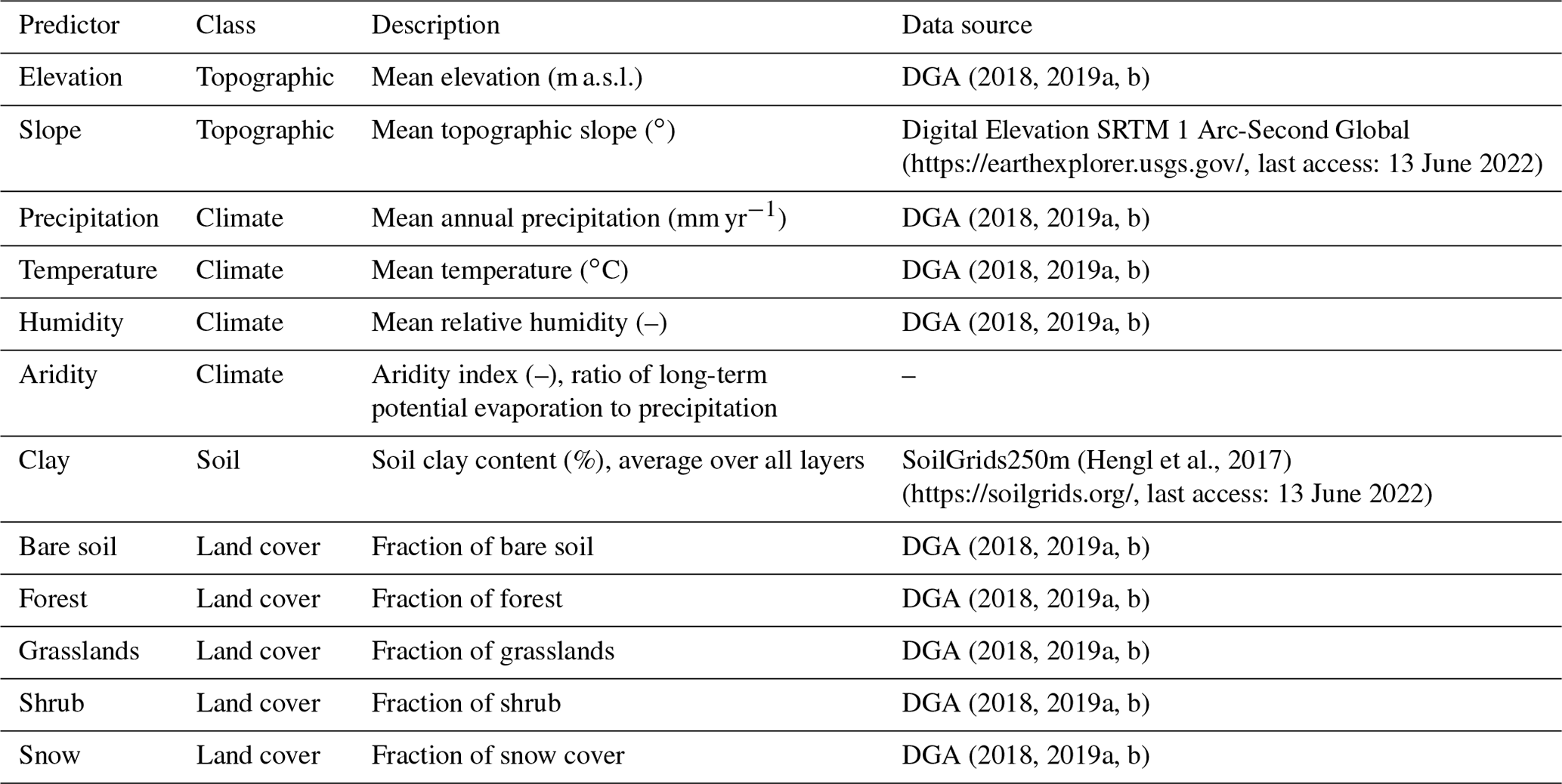
Table 2 List of physiographic and hydroclimatic attributes used to characterize model grid cells.

In this study, meteorological forcing data are obtained from various sources. Time series of daily precipitation and maximum, average and minimum daily temperature are obtained from the CR2MET meteorological dataset (Boisier et al., 2018), introduced in DGA (2017), which provides data for continental Chile at a horizontal resolution of $\mathrm{0.05}{}^{\circ }\times \mathrm{0.05}{}^{\circ }$ (∼5 km) for the period from 1979 to 2016. The precipitation product builds upon a statistical post-processing technique that uses topographic descriptors and simulated meteorological variables from ERA-Interim (Dee et al., 2011) and ERA5 (C3S and Copernicus Climate Change Service, 2017) as predictors and uses daily precipitation records as the predictand. A similar approach is used to generate time series of daily maximum and minimum temperatures, including additional predictors from MODIS land surface products. Daily precipitation and temperature variables are disaggregated into 3-hourly time steps using the sub-daily distribution provided by ERA-Interim. Finally, relative humidity and wind speed were obtained from a blend between ERA-Interim and ERA5, which was subsequently rescaled to the CR2MET horizontal grid through spatial interpolation. It is important to note that this product combination was created because ERA5 was not available during the entire study period (1985–2015) at the time of data acquisition (early 2018, when only 2010–2016 data were available). However, the updated reanalysis information, despite the short time coverage, was included due to various developmental improvements.

3 Methods

3.1 Hydrological model

The Variable Infiltration Capacity (VIC; Liang et al., 1994) model is a semi-distributed, physically based hydrological model that simulates snow accumulation and melt, evapotranspiration (ET), canopy interception, surface runoff, baseflow, and other hydrological processes at daily or sub-daily time steps. While the model was originally designed as a land surface scheme for coupled simulations within Earth system models (Liang et al., 1994), most applications have involved uncoupled simulations for hydrological characterizations; accordingly, the literature reports many attempts to improve process representations (e.g., Liang et al., 1996, 1999; Cherkauer et al., 2003; Andreadis et al., 2009). VIC is predominantly used in the USA (Addor and Melsen, 2019), with many studies focused on water and energy balances (e.g., Andreadis and Lettenmaier, 2006; Cayan et al., 2010); however, its use has expanded to other geographical domains, including China (e.g., Zhao et al., 2013; Gou et al., 2021), Chile (e.g., Vásquez et al., 2021; Vicuña et al., 2021), Europe (e.g., Lohmann et al., 1998; Roudier et al., 2016) and globally (e.g., Shukla et al., 2013; Yang et al., 2021). Ongoing community efforts using the VIC model include the NASA Land Information System (LIS; https://lis.gsfc.nasa.gov/, last access: 25 January 2022), the NASA Land Data Assimilation System (LDAS; https://ldas.gsfc.nasa.gov/, last access: 25 January 2022) and the Regional Arctic System Model (RASM; https://www.oc.nps.edu/NAME/RASM.htm, last access: 25 January 2022). This study uses VIC version 4.1.2.g, which can be downloaded from https://github.com/UW-Hydro/VIC/releases (last access: 13 June 2022), along with other versions.

In VIC, the domain of interest can be spatially discretized into grid cells. Sub-grid land use type variability is accounted for by providing vegetation tiles and the fractional areas, for which water and energy balance equations are solved separately; model states and fluxes are then spatially averaged to provide results at the pixel scale. In VIC, each grid cell can have up to three soil layers: the two top layers represent the interaction between moisture and vegetation, and the bottom soil layer is used to simulate baseflow processes. VIC does not incorporate an aquifer at the bottom of the soil column nor lateral exchange of fluxes between grid cells. Finally, snowpack dynamics are simulated by a two-layer mass and energy balance model (Cherkauer et al., 2003; Andreadis et al., 2009), where the surface layer solves the energy exchange between the snowpack and the atmosphere, and the lower layer stores the excess snow mass from the upper surface layer.

3.2 Parameters considered for sensitivity analysis

We considered a suite of 43 parameters (Table 3) to incorporate most of the soil, vegetation and snow processes simulated by VIC. It should be noted that three of the snow parameters are not exposed to model users (NEW ALB, ALB AA and ALB THA), although the associated relationships and default values were proposed decades ago (USACE, 1956). For parameters with monthly variations, we examined sensitivities using regularization “superparameters” (Tonkin and Doherty, 2005), also called multipliers (Pokhrel and Gupta, 2010), which are uniformly applied over all monthly values. Hence, multipliers are used for the leaf area index (LAI), vegetation albedo (ALB), vegetation roughness length (ROU) and vegetation displacement (DIS). Despite the fact that some of these parameters are considered observable, a non-negligible degree of uncertainty may be involved in their determination; an example of this is the LAI parameter (Tian et al., 2002; Fang et al., 2012, 2013), whose implementation in many hydrology and land surface models is simplified through static monthly values. Assumptions like this motivate us to explore the sensitivity of these types of parameters, which may have the potential to be included in the calibration process.

Table 3 Parameters of the VIC model considered in this study.

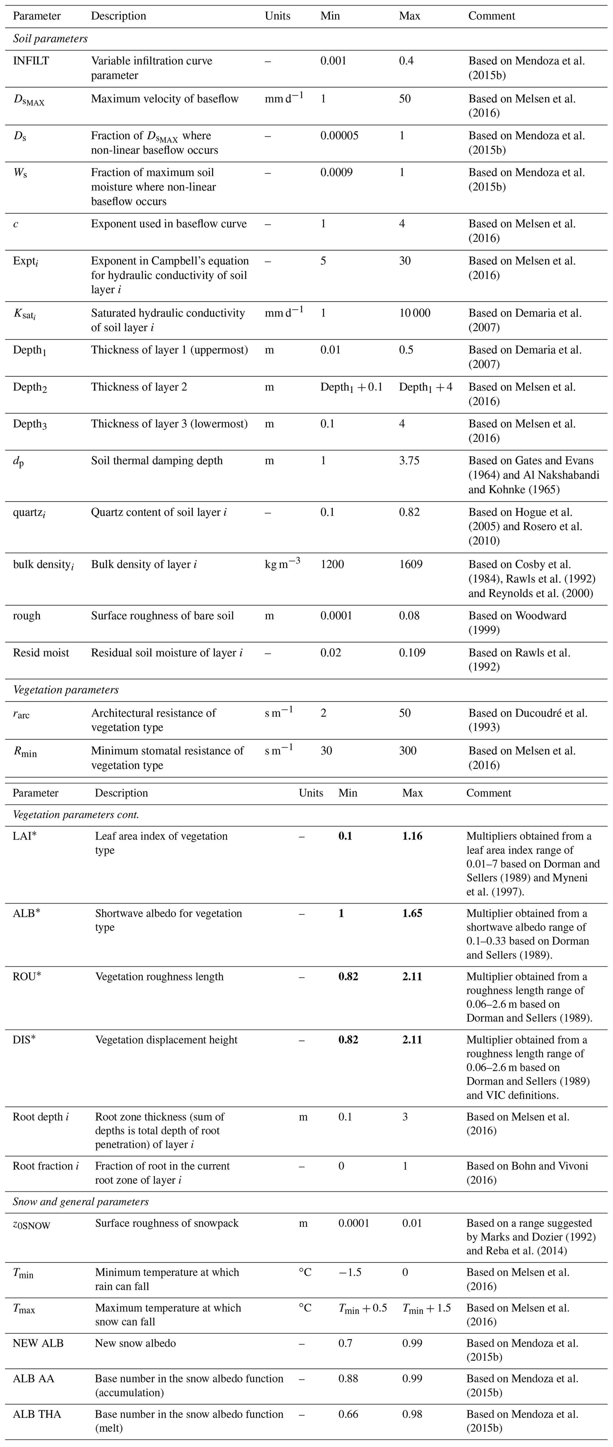
^* This parameter is temporally distributed (monthly variations); therefore, its sensitivity is analyzed based on multipliers. Although the description and units refer to actual parameters of VIC, parameter values in bold represent the multiplier values (instead of actual parameters).

Despite the aim to include the largest possible number of parameters, some of them were discarded for different reasons. For example, a few soil parameters (e.g., soil bubbling pressure) are not active unless the frozen soil algorithm is turned on. We also excluded the “trunk ratio” parameter – i.e., the ratio of total tree height that is trunk (no branches) – because it is activated only in those grid cells with forest (i.e., vegetation class with overstory, spanning 22 % of our study domain) as the land cover type. Finally, we found five mutually related soil parameters that do not allow independent variations: soil bulk density (bd), soil particle density (sd), fractional soil moisture content at the critical point (θ_cr), fractional soil moisture content at the wilting point (θ_wp) and residual soil moisture (θ_r). These parameters are related as follows:

$$\begin{array}{}\text{(1)}& {\mathit{\theta }}_{\mathrm{cr}}\ge {\mathit{\theta }}_{\mathrm{wp}}\ge {\displaystyle \frac{{\mathit{\theta }}_{\mathrm{r}}}{\left(\mathrm{1}-\frac{\mathrm{bd}}{\mathrm{sd}}\right)}}.\end{array}$$

From these five parameters, we only include θ_r and bd, as (1) perturbing θ_r and bd values did not affect numerical solutions, and (2) Bennett et al. (2018) showed that θ_cr, θ_wp, bd and sd did not have substantial effects on model simulations. Finally, those parameters that showed little or no sensitivity in the initial phases of the study were purposely discarded.

3.3 Sensitivity analysis approach

We used the Distributed Evaluation of Local Sensitivity Analysis (DELSA; Rakovec et al., 2014) method, which is a derivative-based, hybrid local–global approach. DELSA combines elements from the method of Morris (1991), the Sobol' method (Sobol', 2001) and regional sensitivity analysis (Hornberger and Spear, 1981), and it provides robust results with fewer model simulations compared with variance-based global methods such as the Sobol' technique. Although DELSA only examines first-order sensitivities, it has unexplored potential to be expanded with the aim of quantifying parameter interactions (Zegers et al., 2020), which could be achieved by including additional terms in the local total variance (Sobol' and Kucherenko, 2010).

Consider a transformation f and a vector θ with k parameters, which provides a metric Ψ describing model output:

$$\begin{array}{}\text{(2)}& \mathrm{\Psi }=f\left(\mathit{\theta }\right),f:R^k\to R.\end{array}$$

Given a sample point θ^* in the parameter space, the gradient for metric Ψ and parameter θ_j around this point – i.e., $\frac{\partial \mathrm{\Psi }}{\partial {\mathit{\theta }}_j}{\mathrm{|}}_{{\mathit{\theta }}^{*}}$ – is considered a measure of local sensitivity. In this work, we follow Rakovec et al. (2014) and compute such a gradient using a forward, finite difference approach with a 1 % change in the parameter value:

$$\begin{array}{}\text{(3)}& {\displaystyle \frac{\partial \mathrm{\Psi }}{\partial {\mathit{\theta }}_j}}{\mathrm{|}}_{{\mathit{\theta }}^{*}}={\displaystyle \frac{\mathrm{\Psi }\left({\mathit{\theta }}_j^{*}+\mathrm{0.01}{\mathit{\theta }}_j^{*}\right)-\mathrm{\Psi }\left({\mathit{\theta }}_j^{*}\right)}{\mathrm{0.01}{\mathit{\theta }}_j^{*}}}.\end{array}$$

In Eq. (3), Ψ(θ^*) is a signature measure of hydrologic behavior, formulated by contrasting model output at the point θ^* with that obtained from a reference parameter set θ^ref in the grid cell of interest (see Sect. 3.3.2 for details). The first-order sensitivity measure for the jth parameter is calculated at each sample point as

$$\begin{array}{}\text{(4)}& S_j^{\mathrm{L}}={\displaystyle \frac{{\left(\frac{\partial \mathrm{\Psi }}{\partial {\mathit{\theta }}_j}{\mathrm{|}}_{{\mathit{\theta }}^{*}}\right)}^{\mathrm{2}}{s}_j^{\mathrm{2}}}{V_{\mathrm{L}}\left({\mathit{\theta }}^{*}\right)}}.\end{array}$$

Here, $s_j^{\mathrm{2}}$ is the a priori parameter variance of the jth parameter, and V_L(θ^*) is the linearized local variance:

$$\begin{array}{}\text{(5)}& V_{\mathrm{L}}\left({\mathit{\theta }}^{*}\right)=\sum _{j=\mathrm{1}}^k{\left({\displaystyle \frac{\partial \mathrm{\Psi }}{\partial {\mathit{\theta }}_j}}{\mathrm{|}}_{{\mathit{\theta }}^{*}}\right)}^{\mathrm{2}}{s}_j^{\mathrm{2}}.\end{array}$$

Finally, $s_j^{\mathrm{2}}$ is obtained from the variance of a uniform distribution (Rakovec et al., 2014), which is $\frac{\mathrm{1}}{\mathrm{12}}{\left({\mathit{\theta }}_{j,\max }-{\mathit{\theta }}_{j,\min }\right)}^{\mathrm{2}}$.

The first-order sensitivity indices vary between zero and one, and the sum of first-order sensitivities from all parameters at each sampling point is equal to one. Local sensitivities can be examined through their cumulative frequency distribution across the parameter space or by computing a specific statistical property. Here, we quantify the relative contribution of a specific parameter using the area above the curve of the full frequency distribution:

$$\begin{array}{}\text{(6)}& {\mathrm{IS}}_j^{\mathrm{L}}=\mathrm{1}-\underset{\mathrm{0}}{\overset{\mathrm{1}}{\int }}F\left(S_j^{\mathrm{L}}\right)d{S}_j^{\mathrm{L}}.\end{array}$$

3.4 Performance metrics

We use eight model evaluation metrics to quantify the sensitivity of simulated hydrological processes to variations in model parameters. The notation, brief description, mathematical formulation and physical process associated with each metric are detailed in Table 4. These metrics are computed by contrasting model output from sampling points produced for DELSA with a reference national-scale dataset with simulated states and fluxes obtained from the national water balance database (DGA, 2018, 2019a, b) for the historical period from 1985 to 2015. This dataset was developed by running the VIC model at the same grid discretization as employed here (i.e., $\mathrm{0.05}{}^{\circ }\times \mathrm{0.05}{}^{\circ }$) and using a combination of CR2MET version 2.0, ERA-Interim and ERA5 output as meteorological forcings. The spatially distributed parameter fields for our reference simulation were developed via parameter regionalization, based on the similarity between possible donor catchments – whose parameters were calibrated individually (Vásquez et al., 2021) – and each grid cell across the domain, following Beck et al. (2016). The reader is referred to Vásquez et al. (2021) and DGA (2018, 2019a, b; in Spanish) for more details on individual model calibration and parameter regionalization procedures used to generate the reference simulation.

Table 4 Parameter sensitivity metrics used in this study.

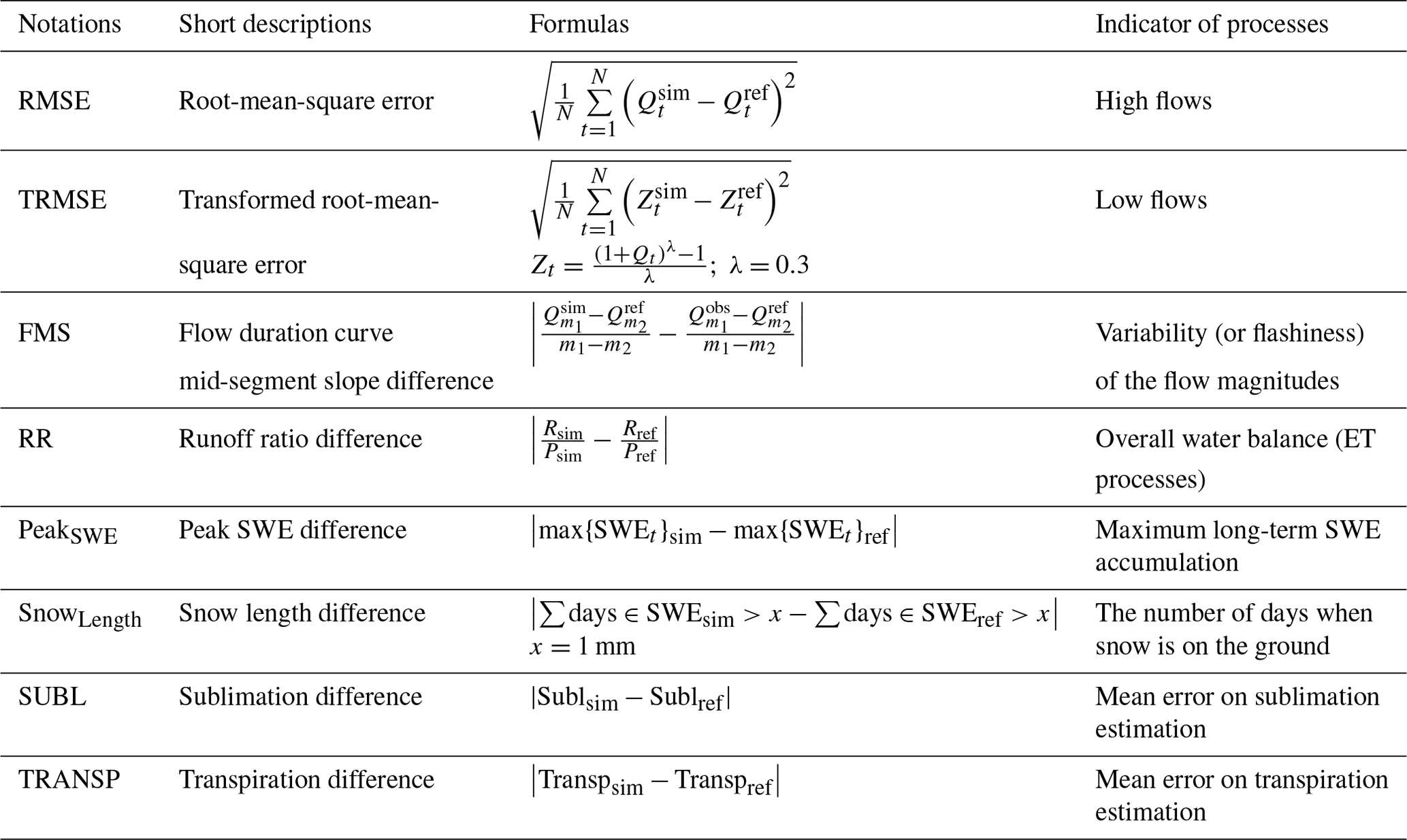
The abbreviations used in the table are as follows: N – number of time steps; Q_t – flow for time step t; Z_t – flow transformed for time step t; $Q_{m_{\mathrm{1}}}$ – m₁ percentile flow of simulated flow duration curve, where m₁=70; $Q_{m_{\mathrm{2}}}$ – m₂ percentile flow of simulated flow duration curve, where m₂=30; R – grid-averaged mean annual runoff; P – grid-averaged mean annual precipitation; SWE_t – snow water equivalent for time step t; Subl – grid-averaged mean annual sublimation; Transp – grid-averaged mean annual transpiration.

Four evaluation metrics are formulated from runoff time series. The first objective function is the root-mean-square error (RMSE), which is a standard metric that emphasizes high flows. The second metric selected is the transformed-root-mean-square error (TRMSE), for which the simulated and observed runoff time series are transformed using a Box–Cox transformation to emphasize low flows (Misirli et al., 2003). The third objective function is the flow duration curve (FDC) mid-segment slope difference (FMS), which represents the variability (or flashiness) of the flow magnitudes; thus, it measures how well a model captures the distribution of the mid-level flows. A steep slope of the FDC indicates flashiness of the streamflow response, whereas a flatter curve indicates a relatively damped response and a higher storage (Yadav et al., 2007; Casper et al., 2012). The fourth evaluation metric is the runoff ratio difference (RR), considered as a measure of the general water balance and, therefore, as a signature of the evapotranspiration model component (Mendoza et al., 2015b).

We use two metrics to characterize snow cover processes: the difference in the long-term simulated peak SWE (Peak_SWE), which is an integrated measure of processes occurring during the snowfall season, and the difference in snow cover duration, quantified by the number of days with snow on the ground (Snow_Length; Mizukami et al., 2014). Finally, we include two metrics based on evaporation fluxes: the sublimation difference (SUBL), which emphasizes the net sublimation from the snowpack surface, and the plant transpiration difference (TRANSP).

3.5 Experimental setup

We apply the DELSA method in 5574 grid cells across continental Chile, which are contained within the 101 catchments described in Sect. 2. In each grid cell, hydrologic model simulations are conducted at 3-hourly time steps for a 12-year period (April 1999–March 2011), with the first 2 years used to initialize model states (i.e., spin-up period). The model is run in full energy balance mode, which means that both energy and water balances are solved, and 3-hourly outputs are aggregated to daily time steps for subsequent analyses.

In this study, we use the Latin hypercube sampling (LHS) method to obtain 200 sample points across the parameter space, for which first-order sensitivity indices are computed. LHS is an efficient simulation technique, especially suitable for statistical and sensitivity calculations (Vořechovský, 2015). To stratify the parameter space, we sample uniformly in a 43-dimensional hypercube and then map onto the parameter space using the inverse cumulative distribution function of each parameter's prior. As DELSA is used here, all parameter distribution functions are assumed to be uniform. The computational cost of applying DELSA at each cell is $N_l(k+\mathrm{1})=\mathrm{8800}$ model runs, where N_l is the number of sample points (200), and k is the number of parameters (43); hence, the total number of models runs required for this study is 49 051 200.

In this paper, a parameter is considered redundant or insensitive when the median value of the integrated first-order sensitivity index (i.e., median IS${}_j^{\mathrm{L}}$) across all grid cells is smaller than 0.05 for at least seven of the eight evaluation metrics listed in Table 4. Parameter sensitivity results are also examined per metric (Sect. 3.4) and grid cell climate type based on the aridity index (Table 5; UNEP, 1997; Verbist et al., 2010).

Table 5 Climate classification used to group model grid cells.

Finally, we use the Spearman rank correlation coefficient (r_s) to measure the degree of association between the parameter sensitivities and physiographic/hydroclimatic characteristics listed in Table 2. These attributes were chosen due to their ability to improve the prediction of hydrological signatures (Addor et al., 2018) and because they are relatively easy to obtain.

4 Results and discussion

4.1 Intra- and inter-basin variability in parameter sensitivities

Figure 3 shows the cumulative distribution functions (CDFs) of sensitivity indices $S_j^{\mathrm{L}}$ for evaluation metric–parameter combinations across six hydroclimatically different catchments – also displayed in Figs. 1 and 2. Each panel located in the first six rows includes the CDFs of all the grid cells contained in a specific basin, and the last row in Fig. 3 comprises the CDFs of all grid cells contained in the six basins. The results reveal high parametric sensitivities for RMSE–INFILT in basins located in northern Chile (arid regime) and lower sensitivities along central and southern catchments, whereas the opposite behavior is observed for TRMSE–$D_{{\mathrm{s}}_{\mathrm{MAX}}}$, FMS–D_s and RR–LAI (i.e., increasing sensitivities towards the south). Such dependence between hydroclimatic basin characteristics and parameter sensitivities was also reported by Demaria et al. (2007). Moreover, Gou et al. (2020) found that sensitivities were strongly related to environmental characteristics, including climate, vegetation, soil and topographic features. Figure 3 also enables the comparison between intra-catchment (top six rows) and inter-catchment (bottom row) variability in parameter sensitivities. For the sample of basins included here, one can note that inter-basin variability in sensitivities is larger than intra-basin variability in runoff-related metrics. Nevertheless, for some metric–parameter combinations, intra-catchment variability is comparable to inter-basin variations in parametric sensitivities. For example, the spread in the CDFs displayed for SUBL–z_0SNOW at basin 8317001 (Biobío River at Rucalhue) – characterized by a wet hydroclimate – is comparable to the spread arising from all basins (see same column, last row).

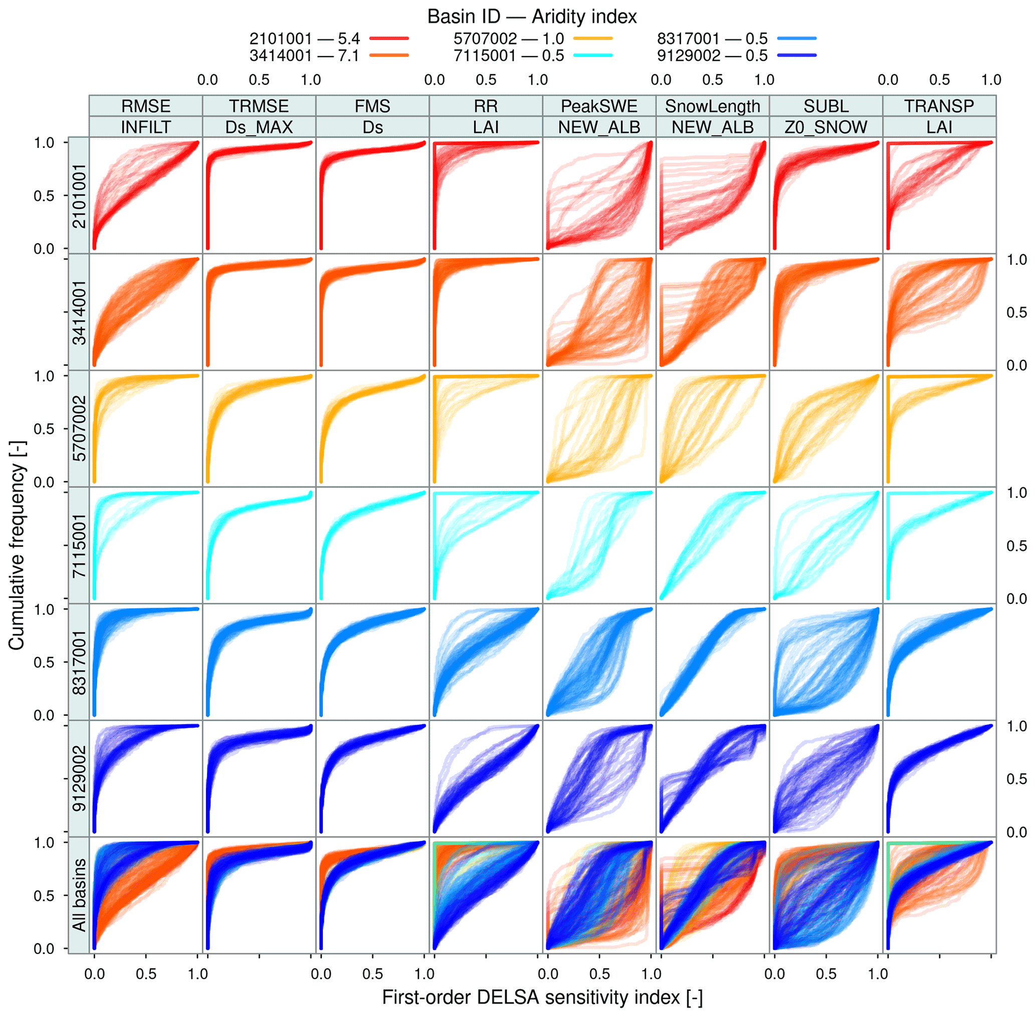
Figure 3 Comparison of cumulative frequency distributions of first-order DELSA indices ($S_j^{\mathrm{L}}$) across six hydroclimatically different basins (displayed in different rows, sorted by latitude). The location and seasonal cycles for these basins are displayed in Figs. 1 and 2, respectively. Results are displayed for the most sensitive parameter associated with each evaluation metric (displayed in different columns); thus, each panel (except those in the last row) comprises the CDFs of all grid cells contained in a specific basin, for a particular metric–parameter combination. The most sensitive parameter was determined based on the median sensitivity index IS${}_j^{\mathrm{L}}$ from all the grid cells contained in the study domain (see text for details). The number next to each basin code at the top of this figure is the catchment-scale aridity index.

To further illustrate intra-basin differences in parameter sensitivities, Figs. 4 and 5 show the spatial distribution of the IS${}_j^{\mathrm{L}}$ indices for the leaf area index (LAI) and the snow albedo parameter ALB THA, respectively, over a cluster of subhumid and humid basins located in southern Chile. For the LAI parameter (Fig. 4), a west–east gradient in IS${}_j^{\mathrm{L}}$ is observed for RMSE (high flows), TRMSE (low flows) and FMS (flashiness of runoff), with increasing sensitivity to LAI variations towards the coast, whereas an inverse pattern is observed for the same metrics and ALB THA (i.e., larger sensitivities towards the Andes, Fig. 5). For Peak_SWE, SUBL and – to a smaller degree – Snow_Length, LAI yields larger sensitivities in vegetated areas, where snow accumulates during winter (Fig. 4), matching those locations where forest is the dominant land cover type, which is also the only vegetation class with an overstory (e.g., trees). Notably, very large variations in Peak_SWE sensitivities to LAI are observed over relatively short distances due to differences among grid cells with respect to the fraction of land cover defined as forest. Such dependence among SWE sensitivities, LAI and canopy fractions was also reported by Bennett et al. (2018). Figure 4 also shows that LAI does not yield a clear sensitivity pattern in RR and TRANSP throughout this subdomain, although IS${}_j^{\mathrm{L}}$ values are higher for RR. For this metric, there are spatial singularities where the sensitivity is minimal or null, as the fraction of ground cover defined as bare soil in these areas increases considerably, reaching up to 100 % bare soil (LAI ∼ 0) in some grid cells.

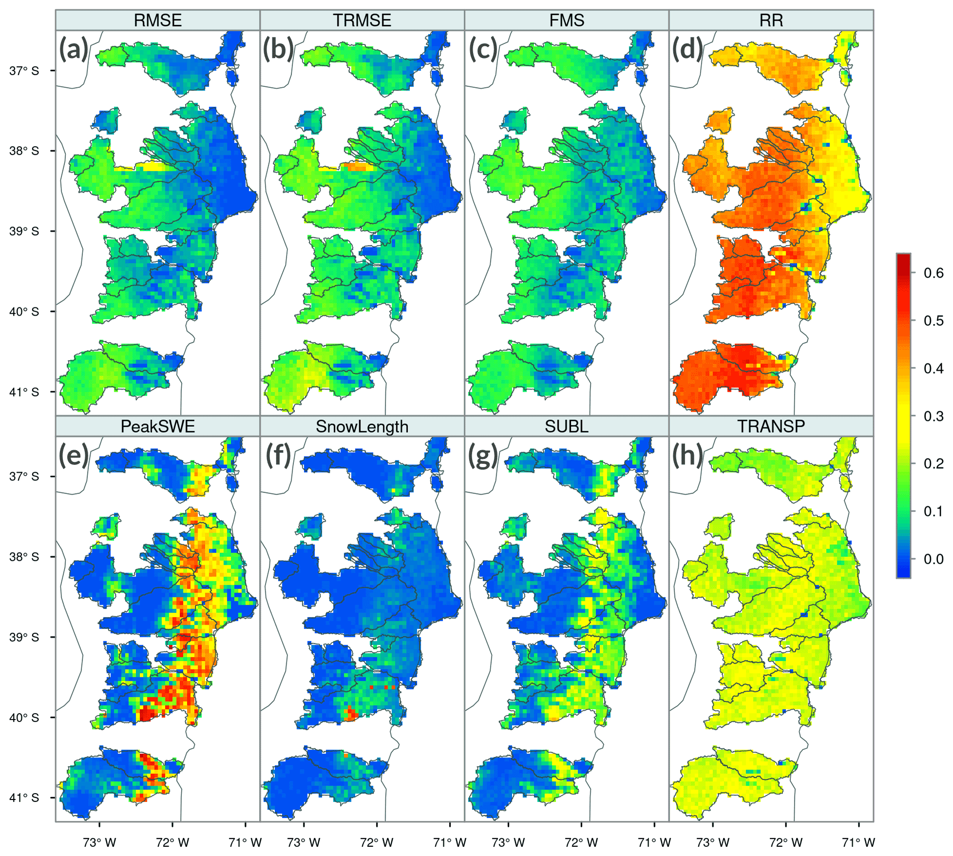
Figure 4 Spatial distribution of integrated first-order DELSA sensitivity indices (IS${}_j^{\mathrm{L}}$) for the leaf area index (LAI) across a humid subdomain located in southern Chile. Results are displayed for eight sensitivity metrics: (a) RMSE, (b) TRMSE, (c) FMS, (d) RR, (e) Peak_SWE, (f) Snow_Length, (g) SUBL and (h) TRANSP.

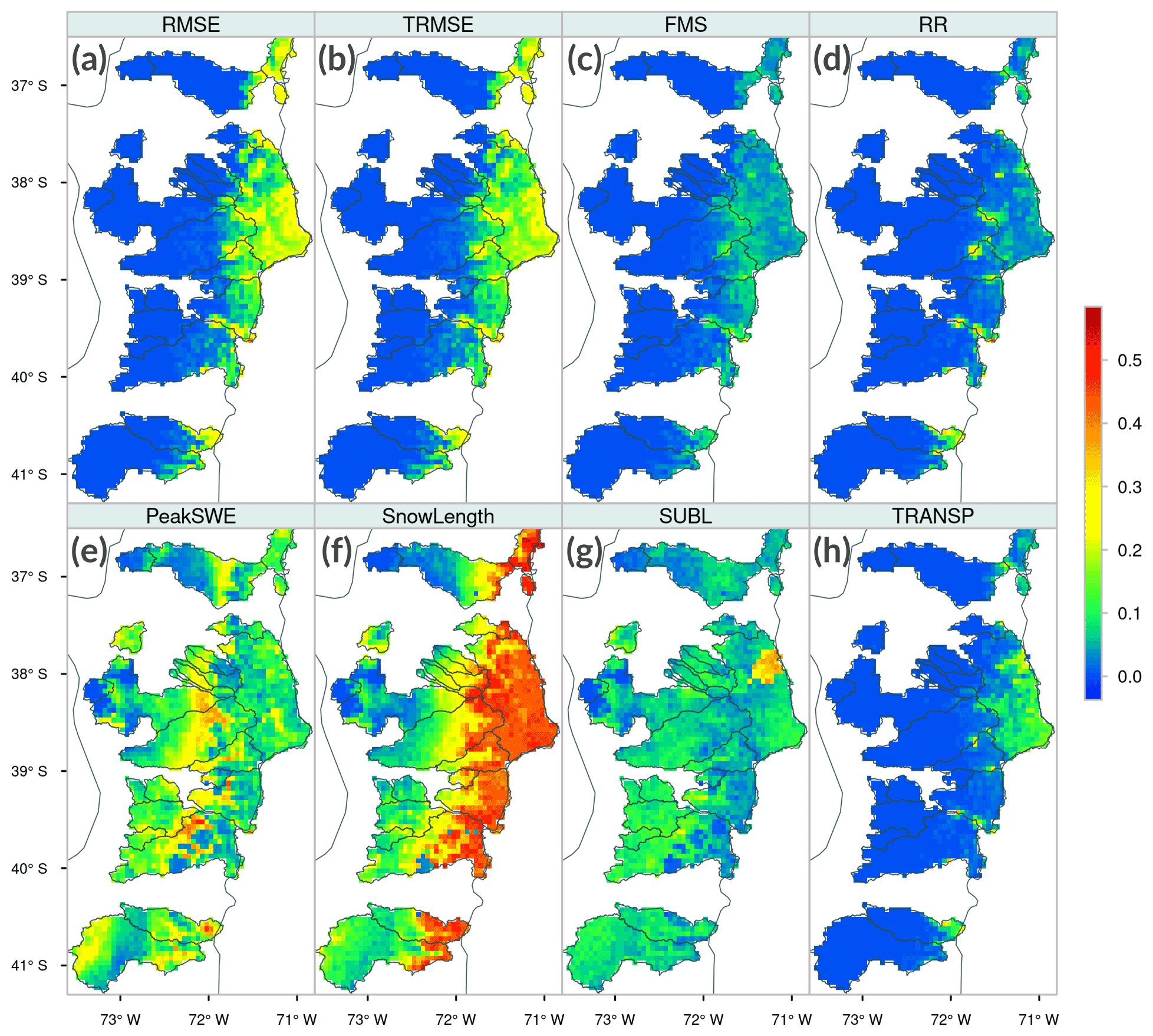
Figure 5 Same as in Fig. 4 but for the base number in the snow albedo function ALB THA (melt).

The results presented in Fig. 5 reinforce the idea that hard-coded parameters should be exposed to users (Mendoza et al., 2015a; Cuntz et al., 2016). In particular, Fig. 5 shows the large effects of ALB THA variations on Snow_Length (with a very pronounced east–west gradient) and, to a smaller degree, on Peak_SWE and SUBL. ALB THA also affects runoff-based metrics along the Andes, especially simulated high (RMSE) and low (TRMSE) flows.

4.2 Identification of the most sensitive parameters

Figure 6 displays box plots comprising IS${}_j^{\mathrm{L}}$ results from all grid cells in the study domain, for each parameter and evaluation metric (displayed in different panels). The results show that 72 % of the parameters analyzed (i.e., 31) yielded small sensitivity indices for the metrics examined here. Conversely, a suite of 12 sensitive parameters are associated with soil (INFILT, D_s, $D_{{\mathrm{s}}_{\mathrm{MAX}}}$, W_s, Expt₂, Depth₂ and Depth₃), snow (NEW ALB, ALB THA and ALB AA) and vegetation (R_min and LAI) processes. Figure 7 shows the spatial variability in IS${}_j^{\mathrm{L}}$ for the 12 parameters identified as the most sensitive across the 101 basins of continental Chile.

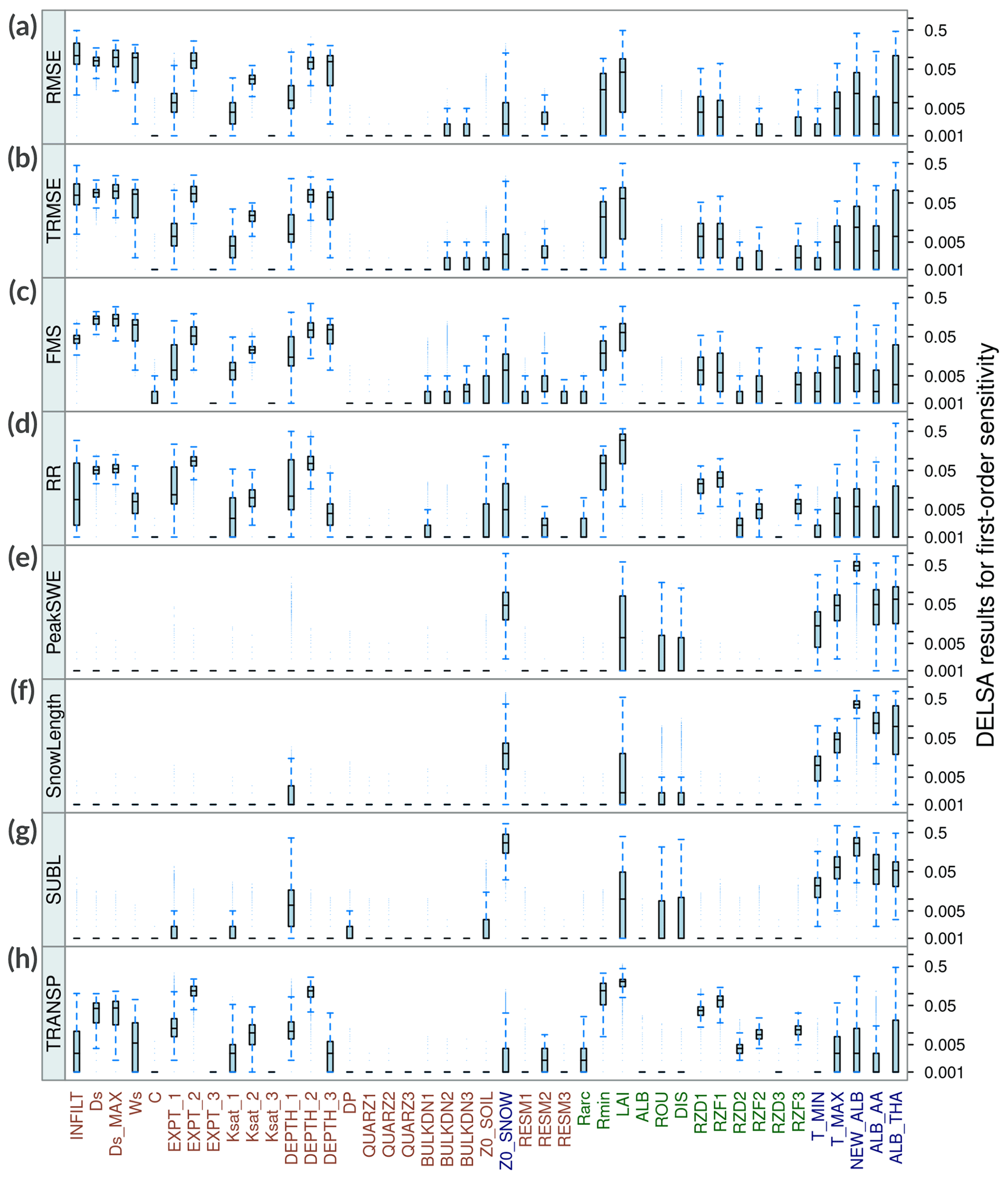
Figure 6 Box plots comprising integrated first-order DELSA sensitivity indices (IS${}_j^{\mathrm{L}}$) from all modeling units (5574 grid cells). Results are displayed for all parameters (x axis) and sensitivity metrics, which are presented in different panels: (a) RMSE, (b) TRMSE, (c) FMS, (d) RR, (e) Peak_SWE, (f) Snow_Length, (g) SUBL and (h) TRANSP.

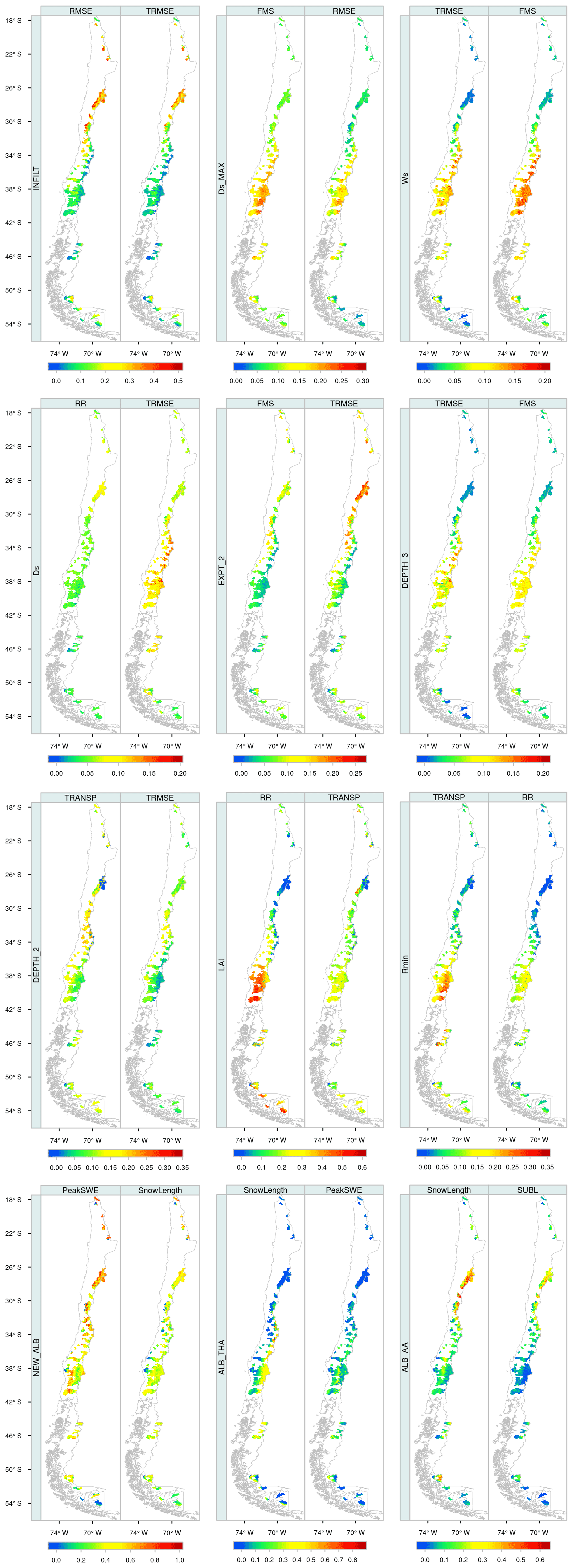
Figure 7 Integrated first-order DELSA sensitivity indices for all grid cells within our study basins. The results are displayed only for the 12 most sensitive parameters as well as their associated most impacted metrics.

For the case of high flows (RMSE), low flows (TRMSE) and flashiness of runoff (FMS), the parameters identified as sensitive are INFILT, D_s, $D_{{\mathrm{s}}_{\mathrm{MAX}}}$, W_s, Expt₂, Depth₂ and Depth₃ (see top three panels in Fig. 6). The INFILT parameter controls the shape of the variable infiltration capacity curve (Zhao et al., 1980; Wood et al., 1992) and, thus, the partitioning of rainfall or snowmelt into infiltration and surface runoff. A higher INFILT value yields less infiltration and higher surface runoff. The RMSE and TRMSE metrics are particularly sensitive to INFILT, indicating a key role in the generation and timing of high and low flows. This parameter has been identified as sensitive in all of the studies listed in Table 1. $D_{{\mathrm{s}}_{\mathrm{MAX}}}$ is the maximum velocity of baseflow, while D_s and W_s are the fraction of $D_{{\mathrm{s}}_{\mathrm{MAX}}}$ and the fraction of the maximum soil moisture content in the third layer, respectively, where non-linear baseflow occurs. These three parameters are involved in the ARNO formulation of subsurface runoff (Franchini and Pacciani, 1991; Todini, 1996), controlling the speed of baseflow release from the third soil layer (Liang et al., 1994) and, specifically, the non-linear part of the baseflow generation function. The sensitivity indices found for these parameters are consistent with the high sensitivity measures reported by Mendoza et al. (2015b), Melsen et al. (2016) and Wi et al. (2017).

The Expt₂ parameter is an exponent of the Brooks–Corey relationship (Brooks and Corey, 1964) and controls the hydraulic conductivity between the second and third soil layers. A small value for the Expt₂ parameter increases inter-layer drainage for the same soil moisture content and, therefore, increases baseflow generation. The Depth₂ parameter is the thickness of the second soil layer. In general, thicker soil layers slow seasonal peak flows and increase water loss due to evapotranspiration (Xie et al., 2007). It should be noted that the parameter Depth₂ has been identified as highly sensitive by many authors (Demaria et al., 2007; Mendoza et al., 2015b; Wi et al., 2017; Gou et al., 2020; Lilhare et al., 2020; Yeste et al., 2020; Melsen and Guse, 2021). Finally, Depth₃ is the thickness of the third layer of soil, and the large sensitivities obtained here agree with the results reported by Mendoza et al. (2015b) and Wi et al. (2017).

The results in Fig. 6 show that Expt₂ and Depth₂ also provide large sensitivities for metrics focused on evaporative fluxes (i.e., RR and TRANSP). Other parameters that are relevant for these processes are LAI and the minimum stomatal resistance (R_min). Indeed, Chaney et al. (2015) reported high sensitivity of annual flow biases to variations in R_min. LAI is a dimensionless quantity that characterizes intra-annual variations in plant canopies, and it is defined as the one-sided green leaf area per unit ground surface area. On the other hand, R_min is one of the parameters that control canopy resistance when computing transpiration from each vegetation class, following the formulations proposed by Blondin (1991) and Ducoudré et al. (1993). Both LAI and R_min provide null sensitivities if the land cover type is bare ground; however, R_min can also produce null sensitivities in vegetated grid cells.

Figure 6 reveals the large influence of hard-coded parameters on Peak_SWE, Snow_Length and SUBL – in particular, NEW ALB, ALB THA and ALB AA. The NEW ALB parameter is the new snow surface albedo, which controls the reflection of solar radiation and, therefore, the energy exchange between the atmosphere, forest canopy and the surface layer of the snowpack (Andreadis et al., 2009). Additionally. The ALB AA and ALB THA parameters represent the albedo decay in the accumulation and melting season in the snow albedo curve, respectively (USACE, 1956). These seasons are defined based on the absence or presence of liquid water in the surface snow cover. These results correspond well with the high sensitivities reported by Mendoza et al. (2015b) for these three hard-coded parameters. Finally, the snow surface roughness length (z_0SNOW) also affects sublimation rates across Andean subdomains.

4.3 What drives parameter sensitivities across different hydroclimates?

Figure 8 shows the Spearman rank correlation coefficient (r_s) between parameter sensitivities and a suite of climatic, topographic, land cover and soil-related grid cell attributes described in Table 2. The magnitude and sign of the correlation quantifies how each sensitivity index varies with a given geophysical attribute. The results show that the magnitude of the correlation varies depending on the metric–parameter combination, with the maximum correlations generally found for soil parameters, such as $D_{{\mathrm{s}}_{\mathrm{MAX}}}$ and W_s, with precipitation (r_s=0.91) and the aridity index ($r_{\mathrm{s}}=-\mathrm{0.91}$) for the FMS function (flashiness of the flow). For this example, the simulation of flow flashiness is highly sensitive to $D_{{\mathrm{s}}_{\mathrm{MAX}}}$ and W_s in the wet region but insensitive in the arid area. Conversely, the minimum correlations are found for snow parameters. It should be noted that a weak correlation indicates that there is less spatial pattern in sensitivity; however, the magnitude of the sensitivity index can be high or low. For example, NEW ALB is a highly sensitive parameter across the domain (Fig. 6).

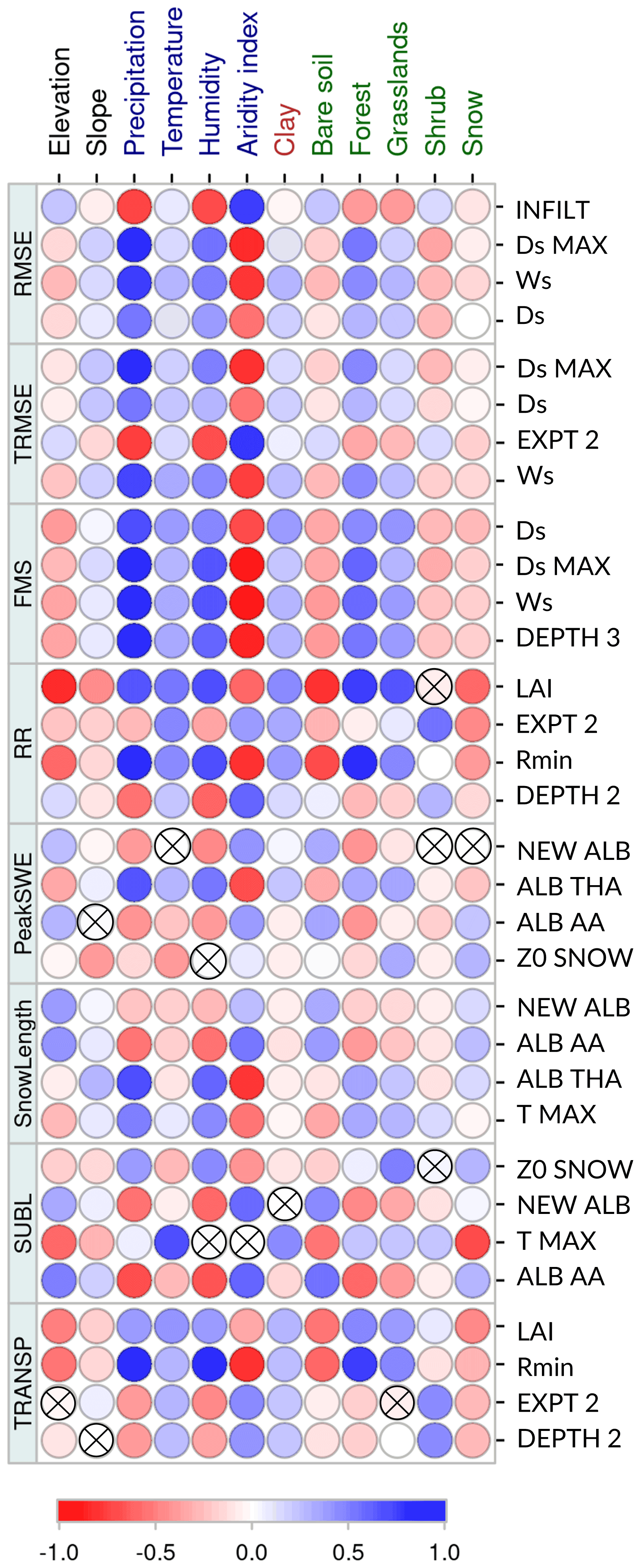
Figure 8 The Spearman rank correlation coefficient between integrated first-order DELSA sensitivity indices IS${}_j^{\mathrm{L}}$ and grid cell characteristics. Results are displayed only for the four most sensitive parameters affecting each metric. The crosses indicate correlations with p values larger than 0.05.

The results in Fig. 8 also indicate that high correlations (either positive or negative) are mainly associated with climate indices, which exert a stronger influence compared with the remaining attribute classes. These strong dependencies of the parametric sensitivity on climate variables are somewhat expected, as some combinations of hydrological signatures and parameters inherit strong spatial climate patterns (Addor et al., 2018); compare, for example, the aridity index, shown in Fig. 1d, with $D_{{\mathrm{s}}_{\mathrm{MAX}}}$–FMS and $D_{{\mathrm{s}}_{\mathrm{MAX}}}$–RMSE, shown in Fig. 7. Among climate descriptors, the aridity index, mean annual precipitation and relative humidity yield the highest correlations, and temperature exhibits a relatively lower influence on parametric sensitivity; this result was confirmed with additional correlation analyses including only grid cells with mean annual temperatures below 5 and 2 ^∘C (not shown). The lowest correlations are obtained for mean slope (topographic attribute), shrub fraction (land cover attribute) and mean clay content of soil (soil attribute). The key influence of climatic conditions on hydrological behavior is not new, as aridity is commonly regarded as the main driver of water partitioning at the land surface (Budyko, 1974; Hrachowitz et al., 2013).

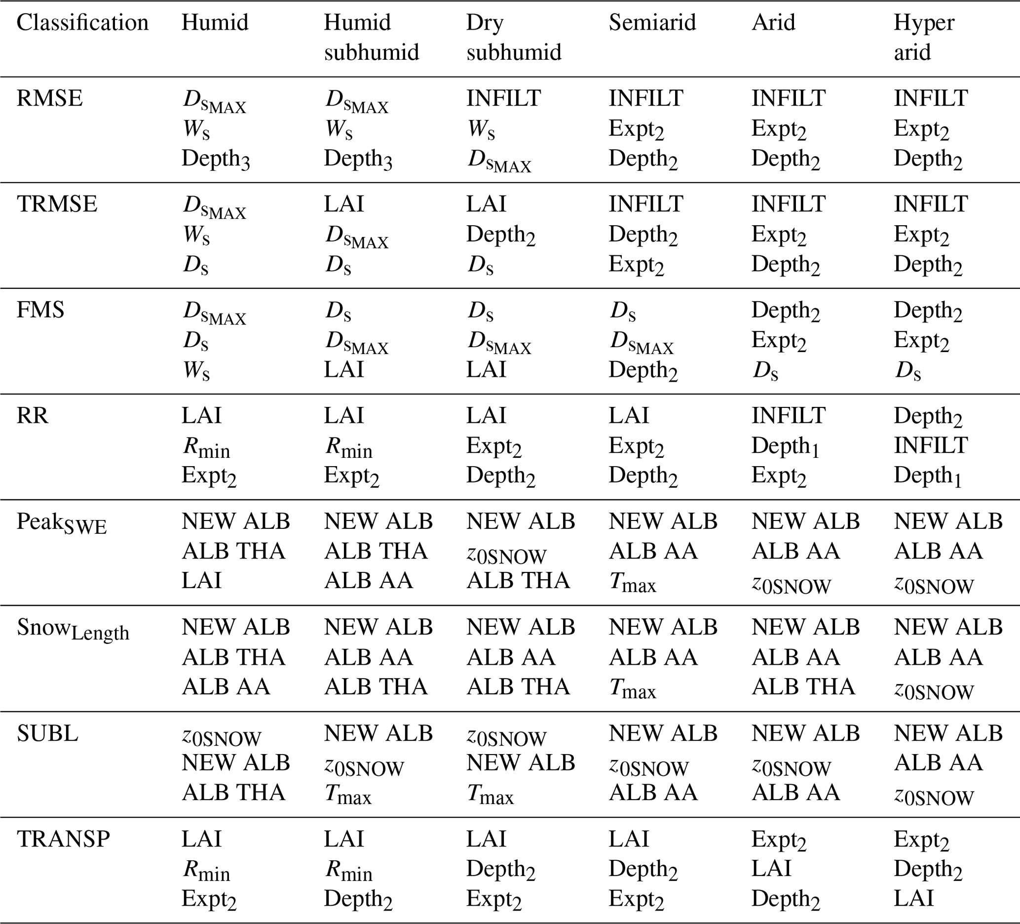
Figure 8 shows that the extent to which parametric sensitivities are related to grid cell attributes depends on the target evaluation metric (i.e., runoff, evaporative processes and snow processes), with the three distinct groups containing the same influential parameters. In the following subsections, we discuss the results based on these groups, with emphasis on spatial patterns and process interpretation across our study basins. Table 6 summarizes, for each evaluation metric (i.e., physical process to be represented) and climatic zone (using the classification from Table 5), the three most important parameters. Hence, the lists contained therein can be used to guide the selection of parameters for hydrologic model calibration, based on the hydroclimatic regime and target process that modelers would like to represent.

4.3.1 Runoff-oriented metrics

The results presented in Fig. 7 (see RMSE and TRMSE) and Fig. 8 (RMSE) show a direct relationship between the sensitivities provided by INFILT, as well as the degree of aridity, especially in semiarid to hyperarid subdomains. The runoff-oriented metrics are also sensitive to baseflow generation parameters D_s, W_s and $D_{{\mathrm{s}}_{\mathrm{MAX}}}$ in most basins – with a similar spatial distribution of IS${}_j^{\mathrm{L}}$ values – except for those located in the north and in some areas of southern Patagonia, where climatic conditions are arid or hyperarid. In basins located in the extreme north, small sensitivities can be attributed to local climate characteristics: most precipitation events in that area occur in summer (i.e., December–March) due to orographic rains caused by air masses coming from the Amazon region, and there is usually little recharge to the aquifers. Additionally, the third soil layer in these basins generally does not reach saturation; therefore, runoff simulations in those areas are insensitive to variations in D_s and W_s because the non-linear part of the baseflow function is only activated when the moisture storage in the third layer exceeds a threshold (Gou et al., 2020). Because of the dependency of $D_{{\mathrm{s}}_{\mathrm{MAX}}}$ on precipitation, this parameter could be playing a key role in the baseflow generation processes over Andean regions (Fig. 7). Finally, a similar spatial distribution of integrated first-order sensitivities for D_s, W_s and $D_{{\mathrm{s}}_{\mathrm{MAX}}}$ is expected, as they all focus on baseflow generation (see $D_{{\mathrm{s}}_{\mathrm{MAX}}}$–FMS, $D_{{\mathrm{s}}_{\mathrm{MAX}}}$–RMSE, W_s–TRMSE, W_s–FMS and D_s–TRMSE in Fig. 7).

Expt₂ is identified as sensitive for runoff-oriented metrics in basins with semiarid to hyperarid climates, characterized by small annual precipitation amounts and permanent water stress. In these hydroclimatic regimes, there is usually not enough water to reach the third soil layer, so water is stored in the second layer and drainage is mainly controlled by Expt₂, affecting the vertical redistribution of soil moisture (FMS) and low flows (TRMSE), as shown in Fig. 7. Depth₂ provides large runoff sensitivities in dry-subhumid to hyperarid hydroclimatic regimes, for the same reasons as Expt₂. Variations in the depth of the second soil layer change the soil moisture of the layer, and higher (lower) values of Depth₂ for the same volumetric water content produce lower (higher) soil moisture, affecting drainage between soil layers.

Table 6 Summary of the most sensitive VIC parameters found for each metric (rows) and climatic type. The three most important parameters are determined based on the median of the integrated first-order DELSA sensitivity indices and are sorted by ranking (i.e., first, second and third most sensitive).

Finally, Depth₃ provides large sensitivities for all runoff-oriented metrics, with similar spatial patterns to W_s, D_s and $D_{{\mathrm{s}}_{\mathrm{MAX}}}$, although to a smaller degree (Fig. 7). Depth₃ is particularly sensitive in humid-subhumid and humid catchments, suggesting a direct relationship with mean annual precipitation or with the size and intermittency of storms (Abdulla and Lettenmaier, 1997). In these climatic domains, periodic heavy-rainfall events enable a continuous recharge of the second and third soil layers – which may reach saturation – and, thus, a constant baseflow generation that affects runoff response and the retention time of soil moisture, producing higher baseflow during wet seasons (Shi et al., 2008). Interestingly, in humid subdomains, baseflow parameters yield high sensitivities in both rainfall- and snowfall-dominated grid cells, although ALB THA emerges as the most important parameter for RMSE and TRMSE in snowfall-dominated grid cells (not shown).

4.3.2 Evaporative processes

The evaluation metrics associated with these processes are RR (a measure of the overall water balance) and TRANSP (plant transpiration), with LAI, R_min, Expt₂ and Depth₂ being the most important parameters.

Figure 7 shows a pronounced spatial variability in LAI sensitivities across a large domain that comprises very different land cover types. One can note that LAI yields high sensitivities for nearly all hydroclimatic regimes, as this parameter controls the evaporation from the canopy layer and canopy transpiration. In hyperarid climates, the LAI is usually less important, given the permanent water stress common for grid cells with bare soil. In summary, LAI is influential wherever vegetation exists, regardless of the prevailing hydroclimatic regime.

The parameter R_min yields parametric sensitivities across humid-subhumid and humid areas (Fig. 7 and Table 6). In the canopy resistance process, there is a stomatal resistance multiplier, g_sm[n], defined as a soil moisture stress factor that depends on the water in the root zone for the nth surface cover class. Thus, when the soil moisture in layer n is less than the fraction of the moisture content at the wilting point, the value of g_sm[n] is zero, whereas when the soil moisture is greater than the fractional content of soil moisture at the critical point (∼70 % of field capacity), the value of g_sm[n] is one. For the intermediate condition, g_sm[n] values vary linearly with soil moisture in that layer, which explains why R_min provides high sensitivities in very humid (i.e., large precipitation) climates.

Finally, our results show that Expt₂ and Depth₂ yield large sensitivities to RR and TRANSP in all hydroclimatic regimes, as they affect the soil moisture content in layer 2, which indirectly affects the g_sm[n] factor in the canopy resistance formulation. These parameters show a lower relative sensitivity in humid/subhumid and humid climates, as the R_min parameter becomes more relevant when there is no soil moisture stress (i.e., g_sm[n]∼1).

4.3.3 Snow processes

Figure 7 shows that NEW ALB, ALB THA and ALB AA yield high sensitivities throughout the study domain, especially in areas where snow processes dominate hydrological responses. In particular, the NEW ALB parameter is important throughout the domain and reaches the highest values for snow-oriented evaluation metrics. Additionally, the results in Fig. 7 show that ALB AA and ALB THA dominate snow responses in different domains: the ALB THA parameter yields large sensitivities in humid and subhumid mountainous areas located south of 34^∘ S, with large effects on the snow season length and the maximum SWE accumulation, whereas ALB AA shows greater sensitivity for the other climatic regimes, affecting Snow_Length and sublimation in semiarid, colder environments in northern Chile (26–29^∘ S).

5 Conclusions

In this study, we have revisited parameter sensitivities in the Variable Infiltration Capacity hydrological model. To this end, we have implemented the DELSA method at every $\mathrm{0.05}{}^{\circ }\times \mathrm{0.05}{}^{\circ }$ (∼5 km) grid cell contained in 101 basins across continental Chile (i.e., a total of 5574 grid cells), spanning a broad diversity of hydroclimatic (from hyperarid to humid) and physiographic (e.g., topography and land cover) conditions. Our experiments consider a suite of 43 parameters included in soil, vegetation and snow process representations, with 3 of these corresponding to hard-coded parameters (i.e., not exposed to model users). We use eight model evaluation metrics that account for runoff components, evapotranspiration and snow processes, and we conduct correlation analyses to disentangle relationships between parametric sensitivities and pixel-scale attributes. The main findings of this study are as follows:

• A total of 31 of the 43 (i.e., 72 %) parameters yield little or no sensitivity, most of which correspond to soil and vegetation processes. Therefore, calibrating such parameters will lead to minimal improvements in system representations with considerable computational costs.

• The three model evaluation metrics focused on snow accumulation and ablation processes were found to be highly sensitive to hard-coded parameters. Exposing these parameters will certainly expand our abilities to perform extensive analysis and increase our opportunities to improve model fidelity and characterize model uncertainty.

• For some evaluation metrics, the climate attributes examined here are highly correlated with parameter sensitivities, which therefore inherit spatial patterns observed in climate variables across the territory. In particular, mean annual precipitation and the aridity index are highly correlated with D_s, W_s and $D_{{\mathrm{s}}_{\mathrm{MAX}}}$ sensitivities when examining RMSE, TRMSE and FMS. Unexpectedly, temperature yields a relatively lower influence among climate descriptors, even for metrics and parameters associated with snow processes. The rest of the attributes (topographic, soil and land cover) provided generally low correlations and, therefore, small predictive power on parameter sensitivities.

• Parametric sensitivities are strongly related to the climate types in the case study basins. In humid environments, the most important parameters are related to the third soil layer (W_s, D_s, $D_{{\mathrm{s}}_{\mathrm{MAX}}}$ and Depth₃) and vegetation (R_min); in arid regimes, the most influential parameters are associated with the first soil layers (INFILT, Expt₂ and Depth₂).

• In snow-dominated areas, the hard-coded parameters NEW ALB, ALB THA and ALB AA provide large sensitivities to maximum SWE, snow season length and sublimation.

• The leaf area index (LAI) is a crucial parameter wherever there is vegetation on the ground. Although such conditions are more frequent in humid environments, the relevance of this parameter depends on vegetation characteristics rather than the underlying climatic conditions.

This study reaffirms overparameterization issues in the VIC model (e.g., Demaria et al., 2007; Gou et al., 2020) as well as the fact that relative parameter importance varies depending on the specific metric or variable analyzed (Chaney et al., 2015; Bennett et al., 2018; Yeste et al., 2020; Melsen and Guse, 2021) and the physiographic or climatic site characteristics (Liang and Guo, 2003; Demaria et al., 2007; Lilhare et al., 2020). However, the results and conclusions reported here are not directly comparable to previous studies due to differences in the experimental designs and domains of interest. In particular, our study considers (1) a large number of soil, vegetation and snow parameters – only comparable to Bennett et al. (2018), who included 46 parameters (excluding snow processes) over the semiarid Colorado River basin; (2) a larger number of process-oriented metrics (compared with the previous efforts listed in Table 1); and (3) a very large sample of grid cells at a relatively high (∼5 km) horizontal resolution, spanning very different physiographic characteristics and hydroclimatic conditions. Hence, our study contributes to the existing literature by providing guidance on relevant VIC parameters for a suite of target processes and climate types.

Future studies aiming at improving spatial calibration density or parameter regionalization techniques using VIC – or any similar hydrology or land surface model – could incorporate this information to define spatially varying target parameters and to examine the extent to which the spatial patterns in parameter sensitivities relate to calibrated parameter fields. Finally, the strong correlations found here between parameter sensitivities and hydroclimatic properties reaffirm the need to incorporate periods with contrasting climate characteristics in sensitivity analysis and calibration strategies in order to achieve more credible hydrologic model simulations under changing climatic conditions.