the Creative Commons Attribution 4.0 License.
the Creative Commons Attribution 4.0 License.
 | 28 Jun 2022
Integrating process-related information into an artificial neural network for root-zone soil moisture prediction
Roiya Souissi
Mehrez Zribi
Chiara Corbari
Marco Mancini
Sekhar Muddu
Sat Kumar Tomer
Deepti B. Upadhyaya
Ahmad Al Bitar
Quantification of root-zone soil moisture (RZSM) is crucial for agricultural applications and the soil sciences. RZSM impacts processes such as vegetation transpiration and water percolation. Surface soil moisture (SSM) can be assessed through active and passive microwave remote-sensing methods, but no current sensor enables direct RZSM retrieval. Spatial maps of RZSM can be retrieved via proxy observations (vegetation stress, water storage change and surface soil moisture) or via land surface model predictions. In this study, we investigated the combination of surface soil moisture information with process-related inferred features involving artificial neural networks (ANNs). We considered the infiltration process through the soil water index (SWI) computed with a recursive exponential filter and the evaporation process through the evaporation efficiency computed based on a Moderate Resolution Imaging Spectroradiometer (MODIS) remote-sensing dataset and a simplified analytical model, while vegetation growth was not modeled and was only inferred through normalized difference vegetation index (NDVI) time series. Several ANN models with different sets of features were developed. Training was conducted considering in situ stations distributed in several areas worldwide characterized by different soil and climate patterns of the International Soil Moisture Network (ISMN), and testing was applied to stations of the same data-hosting facility. The results indicate that the integration of process-related features into ANN models increased the overall performance over the reference model level in which only SSM features were considered. In arid and semiarid areas, for instance, performance enhancement was observed when the evaporation efficiency was integrated into the ANN models. To assess the robustness of the approach, the trained models were applied to observation sites in Tunisia, Italy and southern India that are not part of the ISMN. The results reveal that joint use of surface soil moisture, evaporation efficiency, NDVI and recursive exponential filter represented the best alternative for more accurate predictions in the case of Tunisia, where the mean correlation of the predicted RZSM based on SSM only sharply increased from 0.443 to 0.801 when process-related features were integrated into the ANN models in addition to SSM. However, process-related features have no to little added value in temperate to tropical conditions.
- Article
(16219 KB) - Full-text XML
- BibTeX
- EndNote


Soil moisture is a major land parameter integrated into several agricultural, hydrological and meteorological applications (Koster et al., 2004; Paris Anguela et al., 2008). This essential climate variable (ECV) consists of two components, namely, surface soil moisture (SSM) (0–5 cm) and root-zone soil moisture (RZSM). RZSM corresponds to the soil moisture in the region in which the main vegetation rooting network is developing. Its definition varies depending on vegetation type and pedoclimatic conditions. The importance of RZSM is mainly highlighted in agricultural applications through vegetation stress and water needs and in carbon and nitrogen cycles, as RZSM influences biogeochemical activities in soil (Martínez-Espinosa et al., 2021). RZSM is nonlinearly related to SSM through different hydrological processes, such as diffusion processes. RZSM may be extracted by evaporation at the surface through root extraction or by capillary rises (Calvet et Noilhan, 2000). SSM quantification is achieved through three main sources: in situ measurements, model estimates and remote-sensing-based products. Microwave remote-sensing technologies involving sensors such as Soil Moisture and Ocean Salinity (SMOS) (Kerr et al., 2010), Soil Moisture Active Passive (SMAP) (Entekhabi et al., 2010), Advanced Microwave Scanning Radiometer (AMSR) (Owe et al., 2008) and Advanced Scatterometer (ASCAT) (Wagner et al., 2013) have been employed to retrieve SSM at coarse resolutions. Current satellite sensors can only provide surface soil moisture information because of the shallow penetration depth of spaceborne data (on the order of a few centimeters) (Wagner et al., 2007). Fine-spatial-resolution synthetic aperture radar (SAR) data can also be applied in synergy with optical data to retrieve soil moisture (Zribi et al., 2011; Hajj et al., 2014; Dorigo et al., 2011), but again for surface soil moisture. The International Soil Moisture Network (ISMN) is an exhaustive data-hosting facility focused on soil moisture data and associated ancillary information. The ISMN provides in situ soil moisture measurements collected from operational soil moisture networks worldwide (Dorigo et al., 2011). Various models can be adopted to estimate RZSM, such as land surface models (Surfex) (Masson et al., 2013), Interaction Sol-Biosphère-Atmosphère (ISBA) (Noilhan and Mahfouf, 1996), the Community Land Model (CLM; Oleson et al., 2010) or the Joint UK Land Environment Simulator (JULES) (Best et al., 2011) or dedicated crop models such as Aquacrop (Raes et al., 2009) or Simple Algorithm For Yield Estimate (SAFYE) (Battude et al., 2017). While these models provide the advantage of physical process-based estimates, these estimates depend on the availability and accuracy of ancillary information. Model predictions are often enhanced by the implementation of data assimilation techniques, such as the land data assimilation system (LDAS) (Sabater et al., 2007; Entekhabi et al., 2020).
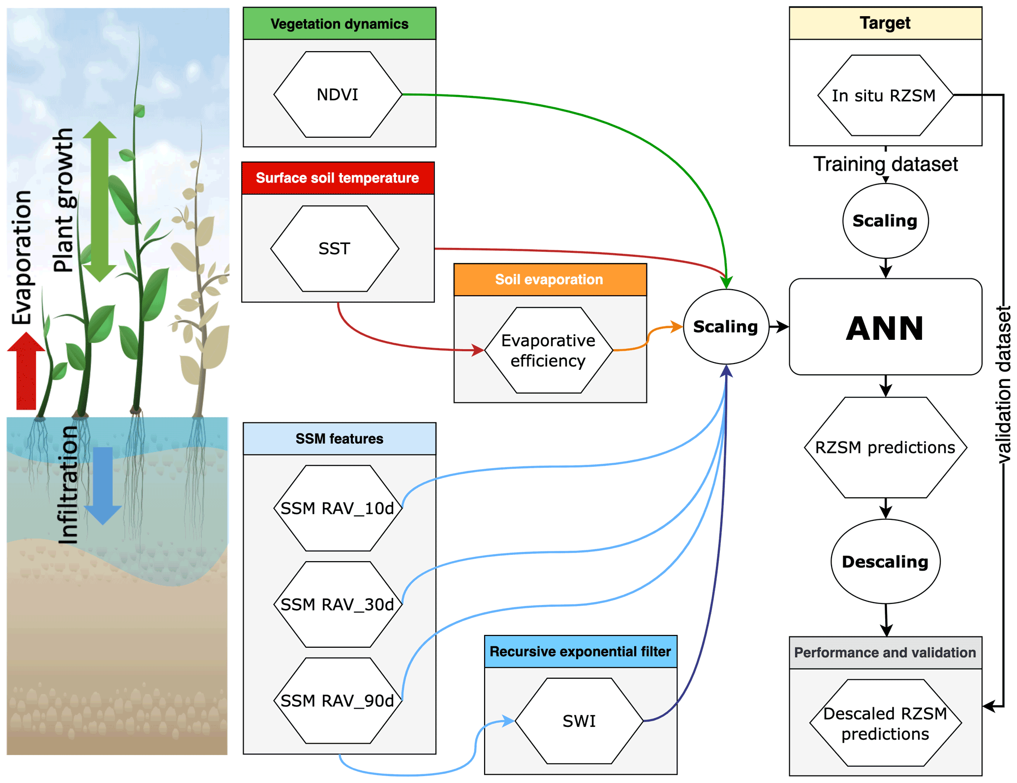
Figure 1Overview of the processing configuration showing the components of the model: the tested models are variations of this ANN with a different combination of inputs (see Table 1). The scaling and descaling are applied to each dataset separately.
Data-driven methods such as artificial neural networks (ANNs) have also been commonly applied in hydrology as detailed, for instance, by the ASCE Task Committee on Application of Artificial Neural Networks in Hydrology (2020) and in Tanty et al. (2015). One of their advantages is that these models do not require an explicit model structure to accurately represent the involved hydrological processes but instead construct a relationship between the given inputs and the process of interest. Therefore, ANNs are regarded as dynamic input–output mapping models heavily relying on the provided training data relevant to target values (Pan et al., 2017). Moreover, ANNs only require a one-time calibration to provide soil moisture estimations once instrument data are loaded and thus generate relatively low computational costs (Kolassa et al., 2018). These advantages explain the approach to estimate RZSM based on surface information with ANNs in various methodologies (Pan et al., 2017; Grillakis et al., 2021; Souissi et al., 2020). In this paper, we do not address ANN applications as a model twin where the ANN model is trained on the target for mimicking purposes and subsequently generates predictions while requiring a short computation time or fewer input simplifications. Here, we are instead interested in the adoption of ANNs as independent models trained on in situ observations. Within this context, Pan et al. (2017) successfully applied an ANN as a model for shallow 20 cm root-zone soil moisture prediction with a global correlation coefficient of 0.7. Grillakis et al. (2021) proposed employing an ANN as a means of calibrating and regionalizing the time constant of a recursive exponential filter, which was thereafter applied at the regional scale. A combined implementation of a Bayesian probabilistic approach and an ANN to infer RZSM at different depths from optical unmanned aerial vehicle (UAV) acquisitions via local training was also applied (Hassan-Esfahani et al., 2017). Multitemporal averaged features to predict RZSM based on only SSM and to investigate the transferability of a trained ANN across different climatic conditions globally were proposed in Souissi et al. (2020). Temporal information can be considered in ANNs through recurrent neural networks (RNNs), long short-term memory (LSTM) architectures (Liu et al., 2021), 1D convolutional neural networks (CNNs), or multitemporal averaging. In Souissi et al. (2020), median, maximum and minimum correlation values of 0.77, 0.96 and 0.65 were, respectively, reported across training, validation and test datasets. The use of climatic variables such as precipitation and surface temperature and intrinsic surface properties such as soil texture and land cover has also been considered in ANNs (Liu et al., 2021). The choice of variables depends not only on the data availability, but also on the objectives. Finally, ANN-based approaches pertain to the more general term of machine learning approaches, and within this framework, the random forest approach has been applied to root-zone soil moisture prediction (Carranza et al., 2021). The aforementioned studies have investigated the application of multiple information sources to predict root-zone soil moisture. The input features are commonly curated for quality, and correlation analysis is conducted to determine the useful inputs, while physical processes are not considered. In this paper, we introduce process-related features based on simplified analytical models representing the major processes contributing to root-zone soil moisture dynamics. In this work, RZSM refers to a point observation of water content at a depth ranging between 30 and 55 cm. We investigate the impact of the application of different process-related variables on the precision of RZSM predictions as well as the robustness of our approach. (1) We start from a previously developed ANN model (Souissi et al., 2020), and we extend the feature list to include NDVI time series, surface soil temperature and process-related variables, namely, the soil water index given by a recursive exponential filter and remote-sensing-based evaporation efficiency. (2) The robustness of the approach is assessed through additional tests involving stations not included in the ISMN database in Tunisia, Italy and southern India. (3) Climatic analysis is conducted to infer the most indicative process-related features for each climate pattern.
The proposed methodology entails the construction of several ANN models with both direct (SSM, surface temperature and NDVI) and intermediate sets of features (soil water index and evaporation efficiency) computed based on simplified analytical models. An overview of the processing configuration is shown in Fig. 1. Standard scaling is applied to each dataset separately so that the different inputs fall into the same range of values. Then the ANN outputs are descaled to make the comparison with actual values of RZSM possible.
This approach results in a combination of ANN models (Table 1). Each model has one or more process-related features in addition to three SSM features which correspond to backward rolling averages of in situ SSM computed over 10, 30 and 90 d. All the ANN model hyperparameters remain the same except the number of input features.
Table 1ANN model configurations with the respective input variables; a: rolling averages of SSM over 10 d; b: rolling averages of SSM over 30 d; c: rolling averages of SSM over 90 d; d: number of parameters of the ANN model.
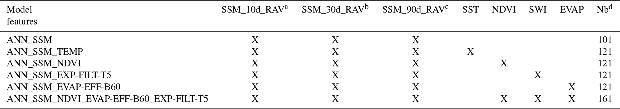
The model with the simplest starting point is ANN_SSM based on Souissi et al. (2020). The most complex model includes the full set of inputs. Intercomparison of the model performance provides information on the added value of each input. All input features are scaled, and training is performed on each of these features based on scaled in situ RZSM data retrieved from the ISMN. The RZSM model predictions are validated against an independent set of observations.
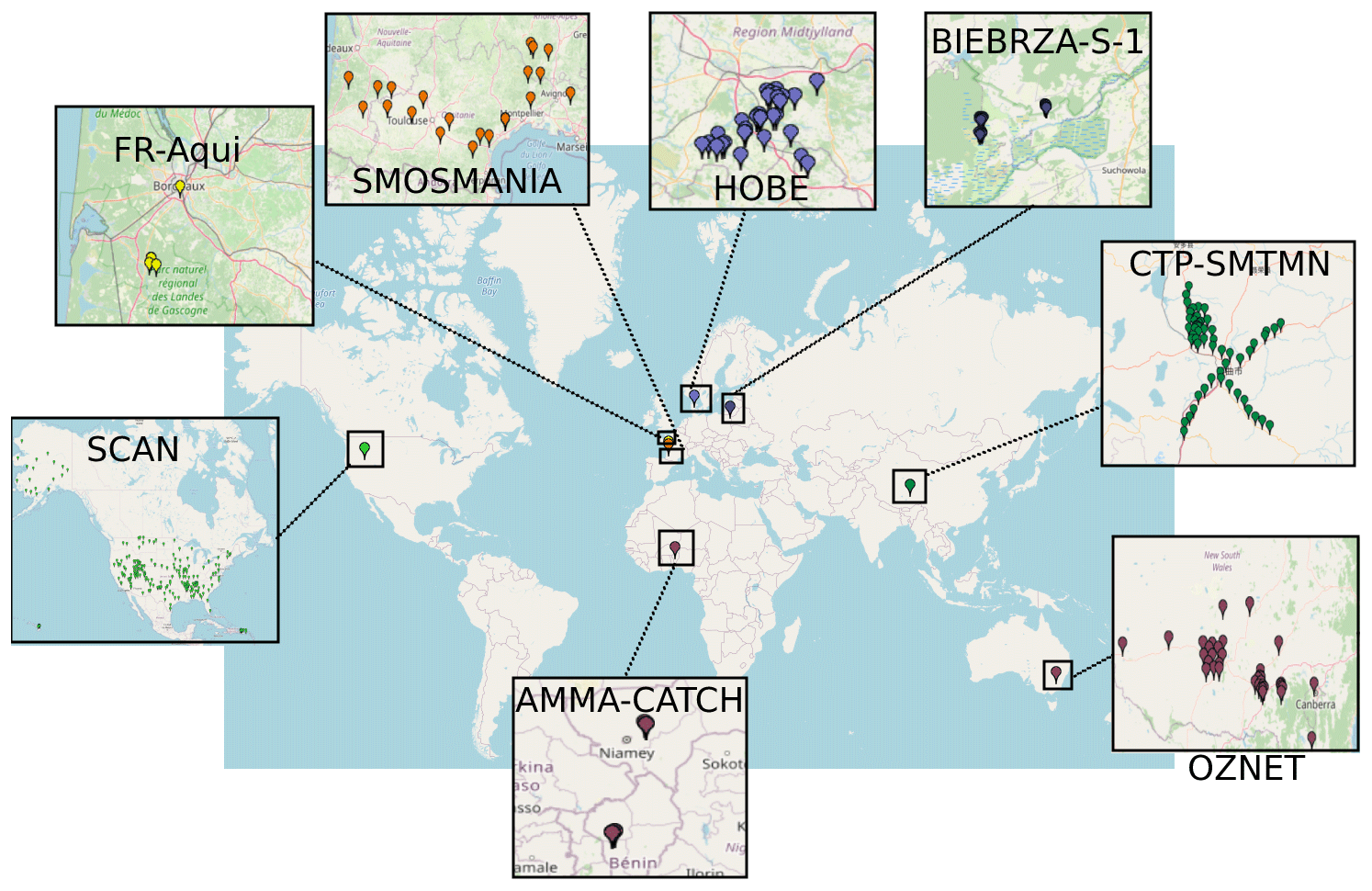
Figure 2International Soil Moisture Network (ISMN) network distribution (adapted from the ISMN web data portal: https://www.geo.tuwien.ac.at/insitu/data_viewer/, last access: 7 April 2022; scale: 1 cm = 1000 km).
2.1 Datasets
2.1.1 ISMN soil moisture data
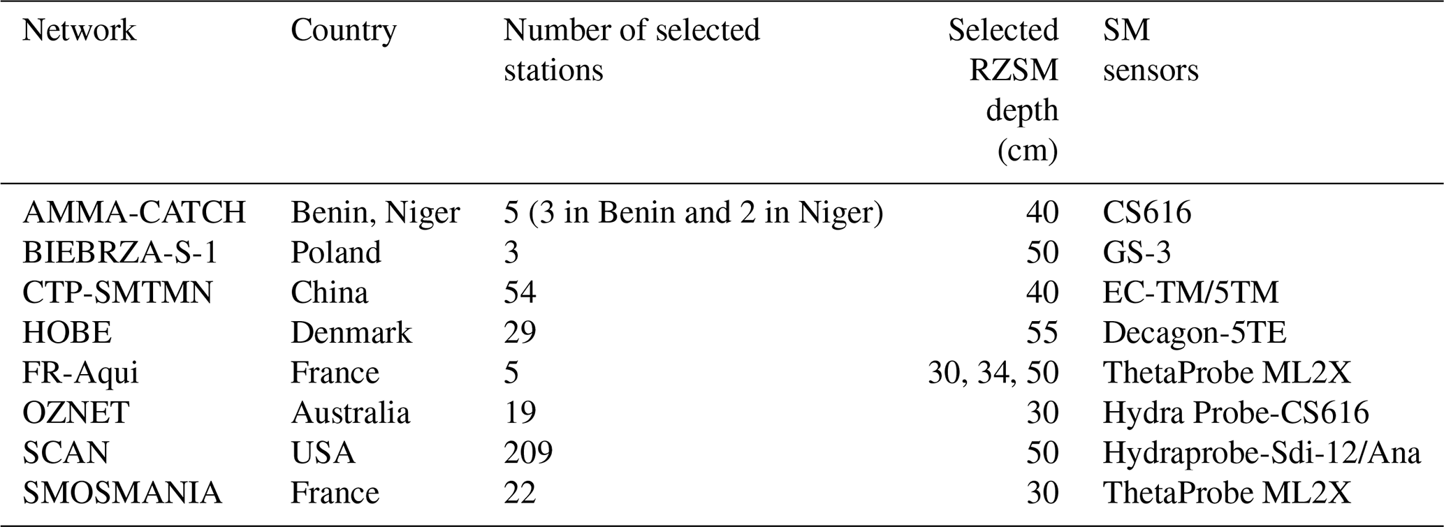
The first training and test operations were conducted on eight ISMN networks previously considered in Souissi et al. (2020). Figure 2 shows the distribution of the considered soil moisture networks with different soil textures and climatic parameters (see Appendix B). For each station, the RZSM observation point is located between 30 and 55 cm (Table 2). For each soil moisture hourly acquisition, the ISMN provides quality flags. Quality flags can be marked as “C” (exceeding the plausible geophysical range), “D” (questionable/dubious), “M” (missing), or “G” (good) (Dorigo et al., 2011). Category “D” has subset flags, namely, “D01” for which in situ soil temperature < 0 ∘C, “D02” that flags points at which in situ air temperature < 0 ∘C, as well as “D03” that also flags areas where the Global Land Data Assimilation System (GLDAS) soil temperature < 0 ∘C. In our study, only soil moisture data whose quality flag is marked “G” were retained.
2.1.2 External soil moisture data
The external networks are considered to assess the transferability and robustness of the approach. The trained models are run for predictions only over these sites. They have been selected to cover semiarid, moderate and tropical semiarid climates.
-
Tunisian site: the Merguellil site is located in central Tunisia (9∘54′ E, 35∘35′ N). This site is characterized by a semiarid climate with highly variable rainfall patterns (average equal to 300 mm yr−1), very dry summer seasons, and wet winters. The Merguellil site represents an agricultural region where croplands, namely, olive groves and cereal fields, prevail (Zribi et al., 2021). At this study site, a network of continuous ThetaProbe stations installed at bare soil locations provided moisture measurements at depths of 5 and 40 cm. All measurements were calibrated against gravimetric estimations. Data were obtained from the Système d'Information Environmental (SIE) web application catalog (SIE, 2021).
-
Italian site: the Landriano site is located in northern Italy (Pavia Province, Lombardy Region). This station is located in a maize field, which was monitored in 2006 and from 2010 to 2011 (Masseroni et al., 2014). The average rainfall in Pavia Province is 650–700 mm, the climate is classified as Cfa (see Appendix A) and the field is irrigated by the border method with an average irrigation amount of approximately 100 to 200 mm per application with one to two applications per season due to the presence of a shallow groundwater table. Soil moisture measurements were performed with time domain reflectometer (TDR) soil moisture sensors. Five TDR soil moisture sensors were installed along a profile at depths of 5, 20, 35, 50 and 70 cm.
-
Indian site: the Berambadi watershed is located in Gundalpet Taluk, Chamarajanagara district, in the southern part of Karnataka state in India and covers an area of approximately 84 km2. The average rainfall is equal to 800 mm yr−1, and the climate is classified as Aw (see Appendix A). Hydrological variables have been intensively monitored since 2009 in the Berambadi watershed by the Environmental Research Observatory ORE BVET and AMBHAS Observatory. The soil moisture levels at the surface (5 cm) and root zone (50 cm) are monitored with a HydraProbe sensor at different agricultural sites across the watershed, and in the current study, four stations were chosen.
2.1.3 Surface soil temperature
In addition to in situ soil moisture, the ISMN optionally includes meteorological and soil variables that are available over specific time periods. Values of the in situ surface soil temperature among these variables can be employed as a useful indicator of the soil moisture data quality. The soil temperature was provided in degrees Celsius, and the plausible values range from −60 to 60 ∘C. Regarding soil moisture data, surface soil temperature data were also provided with quality flags (Dorigo et al., 2011). However, the drawback is that this variable is not available in all networks, which is the case with the AMMA-CATCH network.
2.1.4 Normalized difference vegetation index
We considered the remote-sensing-based normalized difference vegetation index (NDVI) to infer vegetation dynamics. We extracted this index from the Moderate Resolution Imaging Spectroradiometer (MODIS) Vegetation Indices product (MOD13Q1 version 6). MODIS Vegetation Indices data are generated at 16 d intervals and a 250 m spatial resolution as a level-3 product. This product provides two primary vegetation layers. The first vegetation layer is the NDVI, which is referred to as the continuity index of the existing National Oceanic and Atmospheric Administration-Advanced Very High Resolution Radiometer (NOAA-AVHRR)-derived NDVI. The algorithm chooses the best available pixel value from all the acquisitions over the 16 d period. The criteria considered are low cloud coverage, low viewing angle, and the highest NDVI value (Huete et al., 1999). To obtain daily NDVI values, we conducted linear interpolation of the 16 d product.
2.1.5 Potential evapotranspiration
Similarly, we assessed the impact of considering a remote-sensing-based evaporation efficiency, which is initially defined as the ratio of actual to potential soil evaporation, on RZSM prediction. The computation details of this variable will be given later (see Sect. 2.2.2). We employed the remote-sensing-based potential evapotranspiration (PET) to compute the evaporation efficiency. We extracted the PET from the MOD16A2 Evapotranspiration/Latent Heat Flux version 6 product, which is an 8 d composite dataset produced at a 500 m pixel resolution. The algorithm used for this product collection is based on the logic of the Penman–Monteith equation, which employs inputs of daily meteorological reanalysis data along with MODIS remote-sensing data products such as vegetation property dynamics, albedo and land cover. The MOD16A2 product provides layers for the composite evapotranspiration (ET), latent heat flux (LE), potential ET (PET) and potential LE (PLE). The pixel values for the PET layer include the sum of all 8 d within the composite period (Running et al., 2017). To obtain daily PET values, we performed a linear interpolation over the 8 d product, and then we divided the interpolated value by 8.
2.2 Methods
2.2.1 Recursive exponential filter
Two ANN models presented in Table 1 contained extra knowledge on infiltration process information based on the outputs of the recursive exponential filter (Stroud, 1999) as a feature. The recursive exponential filter was first introduced by Wagner et al. (1999) to estimate the soil water index (SWI) from surface soil moisture. SWI is computed as follows:
where SWI is the soil water index at time tn, ms(tn) is the scaled surface soil moisture at time tn (scaled between maximum and minimum values), Kn is the gain at time tn, which occurs in [0, 1] and is given by
and T is a time constant and is the only required tuning parameter to compute the recursive exponential filter.
For the initialization of the filter, gain K1=1 and SWI(t1)=ms(t1).
Regarding T values, we considered an empirical list ([1, 3, 5, 7, 10, 13, 15, 20, 40, 60]), which was partly inspired by Paulik et al. (2014) (T ∈ [1, 5, 10, 15, 20, 40, 60, 100]). Given the list of T values, recursive exponential filter outputs were computed for all of the stations (346 stations) given each T value. Based on the correlation values between the in situ RZSM values and the recursive exponential filter-based RZSM pre-estimates, we established the optimal time variable T, hereafter referred to as Tbest, for each station.
2.2.2 Evaporation efficiency
An ANN model with evaporation efficiency input was also developed. This variable, which is defined as the ratio of the actual to potential soil evaporation, was first introduced in Noilhan and Planton (1989), Jacquemin and Noilhan (1990) and Lee and Pielke (1992) and thereafter readapted in Merlin et al. (2010) to include the soil thickness. In our work, we use a modified evaporation efficiency formulation based on the third model developed in Merlin et al. (2010), which can be expressed as follows (see Appendix C):
where β is evaporation efficiency and θ is the water content in the soil layer of thickness L. θmax is the maximum soil moisture at each station. P* is a parameter computed as follows:
P*, a proxy of parameter P (see Appendix C), represents an equilibrium state controlled by retention forces in the soil, which increase with the thickness L of considered soil and by evaporative demands at the soil surface. PET is the potential evapotranspiration extracted from the MODIS 500 m 8 d product (MOD16A2).
The soil evaporation efficiency computed by model 3, developed in Merlin et al. (2010), decreases when PET increases. Retention force and evaporative demand make the term P increase (replaced by P*), as if an increase in potential evaporation LEp (here replaced by PET) at the soil surface would make the retention force in the soil greater.
Merlin et al. (2010) tested this approach at two sites in southwestern France using in situ measurements of actual evaporation, potential evaporation, and soil moisture at five different depths collected in summer. Model 3 was able to represent the soil evaporation process with a similar accuracy to the classical resistance-based approach for various soil thicknesses up to 100 cm. Merlin et al. (2010) affirm that the parameterization of P as a function of LEp (here PET) indicates that β cannot be considered a function of soil moisture alone since it also depends on potential evaporation. Moreover, the effect of potential evaporation on β appears to be equivalent to that of soil thickness on β. This equivalence is physically interpreted as an increase in retention forces in the soil in reaction to an increase in potential evaporation.
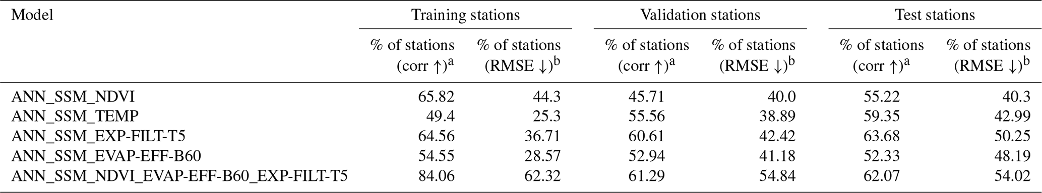
Table 3Proportion of the stations whose performance enhances using the ANN models enriched with process-related features compared to model ANN_SSM (a: % of stations at which the correlation improves over the model ANN_SSM level; b: % of stations at which RMSE improves over the model ANN_SSM level).
2.2.3 Artificial neural network implementation
The multilayer perceptron (MLP), which is a multilayer feed-forward ANN, is one of the most widely applied ANNs, mainly in the field of water resources (Abrahart and See, 2007). The multilayer perceptron contains one or more hidden layers between its input and output layers. Neurons are organized in layers such that the neurons of the same layer are not interconnected and that any connections are directed from the lower to upper layers (Ramchoun et al., 2016). Each neuron returns an output based on the weighted sum of all inputs and according to a nonlinear function referred to as the transfer or activation function (Oyebode and Stretch, 2019). The input layer, consisting of SSM values and/or other process-related variables, is connected to the hidden layer(s), which comprises hidden neurons. The final ANN-derived estimates of the ANN are given by an activation function associated with the final layer denoted as the output layer, based on the sum of the weighted outputs of the hidden neurons.
We started with the ANN model developed in Souissi et al. (2020), whose architecture consists of one hidden layer of 20 hidden neurons, a tangent sigmoid function as the activation function of the hidden layer, a quadratic cost function as the loss function and the stochastic gradient descent (SGD) technique as the optimization algorithm. This model was developed to estimate RZSM based on only in situ SSM information. SSM was not applied as a feature of hourly values but was employed in the form of three features, namely, SSM rolling averages over 10, 30 and 90 d. Additional ANN models were developed to study, through each model, the impact of the application of the NDVI, SWI, evaporation efficiency and surface soil temperature as features. A model combining surface soil moisture, NDVI, evaporation efficiency and the recursive exponential filter was further considered. These ANN models were trained and validated on the 122 ISMN stations considered to be of good quality after a data-filtering step as detailed in Souissi et al. (2020). Training of the above ANN models was conducted considering 70 % of these 122 stations. Thirty percent was reserved for validation, and testing was conducted at the rest of the stations. So, in summary, 122 stations were considered for the training/validation of the ANN models and 224 stations if all input data available were used for testing. In a second step, tests were conducted on data external to the ISMN database, namely, on sites of Tunisia, Italy and India. The trained models over the ISMN are used only in prediction mode over these sites. The data for SSM in addition to the other features are used as inputs, and RZSM is predicted in outputs.
3.1 Exponential filter characteristic time length
A large proportion of the stations attained an optimal time constant (Tbest) value equal to 60 d, which suggests an abnormally long infiltration time. These stations belong to the SCAN network and exhibit an RZSM acquisition depth of 50 cm, in contrast to other networks such as SMOSMANIA, for instance, where RZSM is retrieved at 30 cm. The high values correspond to correlation with seasonal dynamics rather than infiltration processes. This depth could explain the anomalously long infiltration time. This is consistent with Paulik et al. (2014), in which the average T value with the highest correlation (Tbest) increased with increasing depth of the in situ observations.
For comparison purposes, Paulik et al. (2014) found that 23.98 % of the stations achieved Tbest=5 d, while 21.58 % of the stations achieved Tbest≥60 d (60 or 100 d).
Albergel et al. (2008) considered an average Tbest value of 6 d for the SMOSMANIA network. This value represented the average Tbest value for all stations belonging to the SMOSMANIA network. In our case, the average Tbest value for all stations of the SMOSMANIA network reached 9 d. In this study, an average Tbest value could be established for each station or each network. However, this is not relevant to our work because we aim to evaluate maps of remote-sensing data in the next steps, and thus we did not compute Tbest at each location. We fixed the value of T to 5 d as a median infiltration time.
3.2 Intercomparison of the ANN models
The distribution histograms for training, validation and test stations (Fig. 3) show that the integration of the considered process-related features improved the prediction accuracy in certain cases compared to the reference. Time series of good and less good quality of fit were provided in Appendix E for training, validation and test stations using the reference model ANN_SSM and the most complex ANN model.
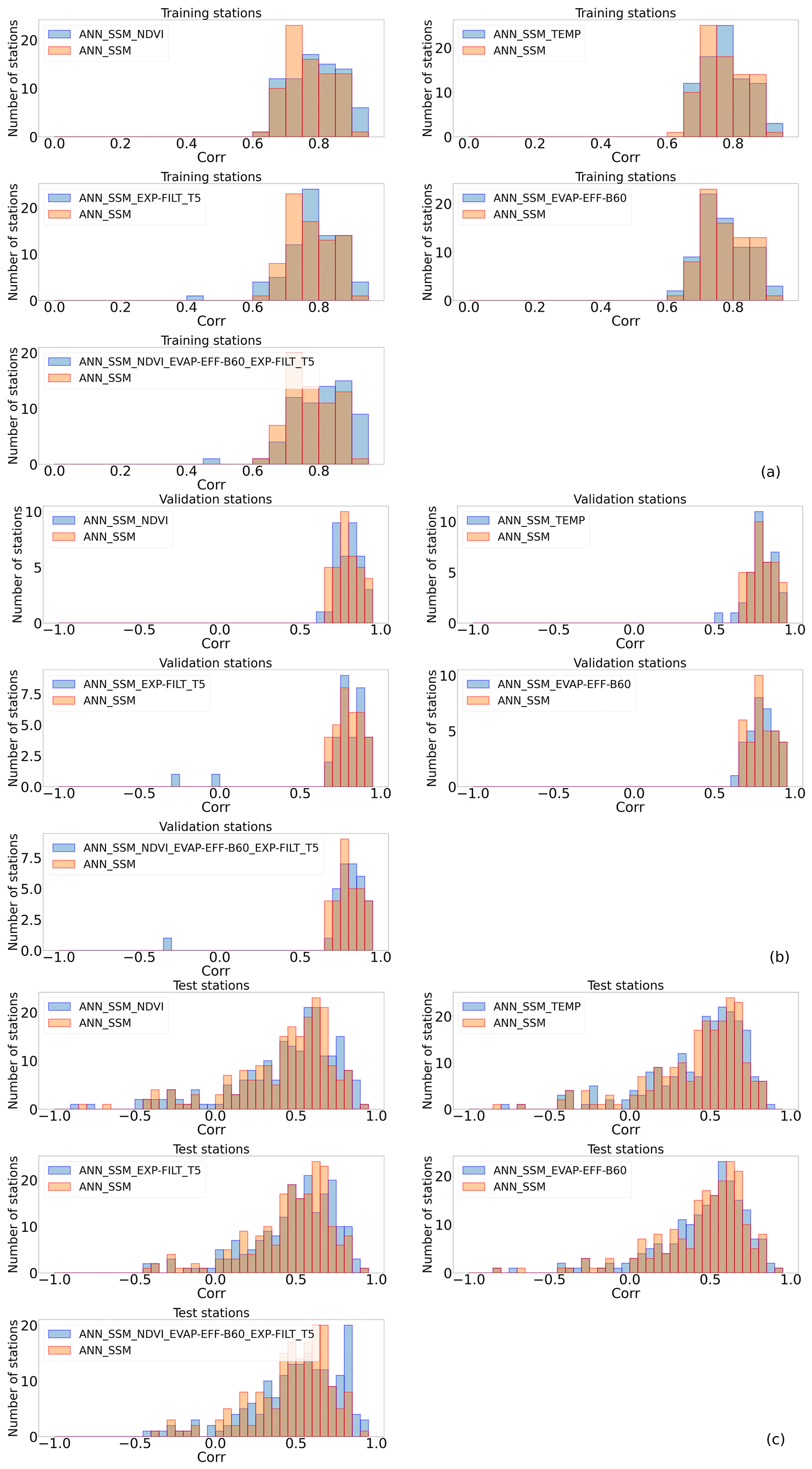
Figure 3Correlation histograms of all tested ANN models compared to ANN_SSM (a) on training stations (b), on validation stations (c) and on test stations (see Appendix D for RMSE histograms).
In terms of the NDVI, 65.82 %, 45.71 % and 55.22 % of the stations attained better correlation values with ANN_SSM_NDVI than those obtained with ANN_SSM for the training, validation and test stations, respectively. Root mean square error (RMSE) decreased for 44.3 %, 40.0 % and 40.3 % of the stations with ANN_SSM_NDVI compared to model ANN_SSM for the training, validation and test stations, respectively (Table 3).
In regard to the ANN_SSM_TEMP model that integrates the soil surface temperature, 49.4 %, 55.56 % and 59.35 % of the training, validation and test stations exhibited higher correlation values than those obtained with the ANN_SSM model, respectively. RMSE decreased with ANN_SSM_TEMP compared to model ANN_SSM for 25.3 %, 38.89 % and 42.99 % of the training, validation and test stations, respectively.
64.56 %, 60.61 % and 63.68 % of the training, validation and test stations attained better correlations than those obtained with model ANN_SSM, respectively. In addition, RMSE decreased for 36.71 %, 42.42 % and 50.25 % of the training, validation and test stations with ANN_SSM_EXP-FILT-T5 compared to model ANN_SSM, respectively.
Regarding the evaporation efficiency, we considered different values of the fitting parameter B (Eq. 4) such that B remained within the [50, 60] interval. This parameter can be fitted using different variables, such as the wind speed or relative humidity. Comparisons based on the correlation values provided by the different models for each B value indicated that the performance was insensitive to the B value. Thus, we fixed the B value to 60 W m−2. Comparison of models ANN_SSM and ANN_SSM_EVAP-EFF-B60 revealed that 54.55 %, 52.94 % and 52.33 % of the training, validation and test stations attained higher correlation values with the latter model, respectively. RMSE was reduced for 28.57 %, 41.18 % and 48.19 % of the training, validation and test stations with ANN_SSM_EVAP-EFF-B60 compared to model ANN_SSM, respectively.
Finally, we investigated the impact of the joint application of the NDVI, recursive exponential filter (T=5 d) and evaporation efficiency (B=60 W m−2) in the ANN_SSM_NDVI_EVAP-EFF-B60_EXP-FILT-T5 model. The surface soil temperature was not included, as its effect is included in the evaporation process. At 84.06 %, 61.29 % and 62.07 % of the training, validation and test stations, the correlation value obtained with this model was higher than that obtained with the ANN_SSM model, respectively. In addition, RMSE was minimized for 62.32 %, 54.84 % and 54.02 % of the training, validation and test stations with ANN_SSM_NDVI_EVAP-EFF-B60_EXP-FILT-T5 compared to model ANN_SSM, respectively.
Considering model ANN_SSM_NDVI_EVAP-EFF-B60_EXP-FILT-T5, only one training station had a decrease in correlation by more than 0.1, namely, station “Lind#1” (network “SCAN”) compared to the reference model ANN_SSM. All inputs were not available at the same dates, which implied a significant reduction in data points (see Appendix F). The decrease in correlation and increase in RMSE did not exceed 0.1 and 0.01 m3 m−3, respectively, for the rest of the stations of lower performance metrics with the most complex ANN (Table 4).
Table 4Proportion of the stations whose correlation decreases using the ANN models enriched with process-related features compared to model ANN_SSM (; X denotes one or a combination of process-related variables)
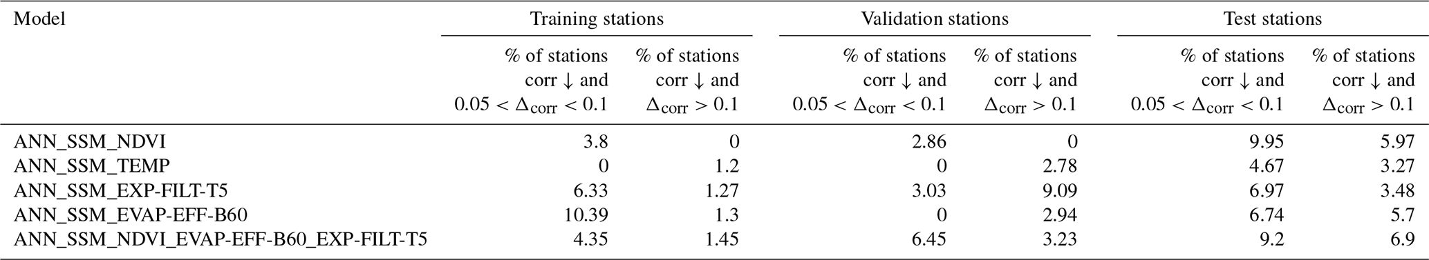
Similarly for validation stations, only one station had a decrease in correlation above 0.1, namely, station “PineNut” (network SCAN), with model ANN_SSM_NDVI_EVAP-EFF-B60_EXP-FILT-T5. This decrease can be also explained because of data shortage (see Appendix F). The decrease in correlation and increase in RMSE did not exceed 0.1 and 0.01 m3 m−3, respectively, for the rest of the stations of lower performance metrics with the most complex ANN (Table 4).
Regarding the test stations, correlation decreased by more than 0.1 and RMSE increased by more than 0.01 m3 m−3 with model ANN_SSM_NDVI_EVAP-EFF-B60_EXP-FILT-T5 compared to model ANN_SSM, detected for only two stations. Both stations, namely, stations “S-Coleambally” and “Widgiewa”, which belong to network “OZNET”, significantly lose in data volume when process-related variables are integrated into ANN and more precisely because of NDVI data availability (see Appendix F). For the rest of the test stations, correlation decreased and RMSE increased simultaneously by less than 0.1 and 0.01 m3 m−3, respectively, with model ANN_SSM_NDVI_EVAP-EFF-B60_EXP-FILT-T5 (Table 4).
Always in terms of the general performance of model ANN_SSM_NDVI_EVAP-EFF-B60_EXP-FILT-T5, about 75 % of the stations have an RMSE of less than 0.05 m3 m−3, and around half of the stations have an RMSE of less than 0.04 m3 m−3. This accuracy is consistent, for instance, with the target value in the SMAP (Entekhabi et al., 2010) and SMOS (Kerr et al., 2010) missions, which is equal to 0.04 m3 m−3, and also with the average sensor accuracy adopted by Dorigo et al. (2013), which is equal to 0.05 m3 m−3. Overall, the most complex model ANN_SSM_NDVI_EVAP-EFF-B60_EXP-FILT-T5 can successfully characterize the soil moisture dynamics in the root zone since half of the stations have a correlation value of greater than 0.7. Pan et al. (2017) developed different ANN models to estimate RZSM at depths of 20 and 50 cm over the continental USA using surface information. They found that half of the stations have an RMSE of less than 0.06 m3 m−3 and that more than 70 % of stations have a correlation above 0.7 when predicting RZSM at 20 cm. However, the developed ANN was less effective in RZSM prediction at 50 cm, which is also in accordance with Kornelsen and Coulibaly (2014). In our study, the densest soil moisture network is SCAN, located in the USA. Soil moisture was predicted at a depth of 50 cm over this network. Around half of the stations have a correlation value of above 0.6 and an RMSE of less than 0.04 m3 m−3 after the integration of process-related inputs. Pan et al. (2017) suggest that the use of only time-dependent variables may not be sufficient for the ANN models to accurately predict RZSM and suggest adding soil texture data.
3.3 Robustness of the approach
To further assess the robustness of our approach, which involves RZSM prediction using the different ANN models with different features, we predicted RZSM at sites not previously considered in previous parts of the study. The selected stations are located in the Kairouan Plain, a semiarid region in central Tunisia, the Landriano site located in the north of Italy, and the Berambadi watershed located in Gundalpet Taluk, southern India. In the case of Tunisia, model ANN_SSM yielded moderate to low-precision predictions, as highlighted by the performance metrics listed in Table 5. The time series (see Appendix G) show that the RZSM predictions followed the SSM seasonality, which was reflected by the false peaks generated in the RZSM predictions whenever a sharp increase or decrease occurred in the SSM values. This observation was also found in Souissi et al. (2020). Actually, the Kairouan Plain is characterized by a semiarid environment where rainfall events infrequently occur and the level of evaporation is high. The reference model ANN_SSM shows its limitations in accurately predicting RZSM in areas with no alternate wet and dry cycles.
Table 5Performance metrics of models ANN_SSM and ANN_SSM_NDVI_EVAP-EFF-B60_EXP-FILT-T5 at training stations of climate “Bsk” and Tunisian stations of climate “Bsh”.
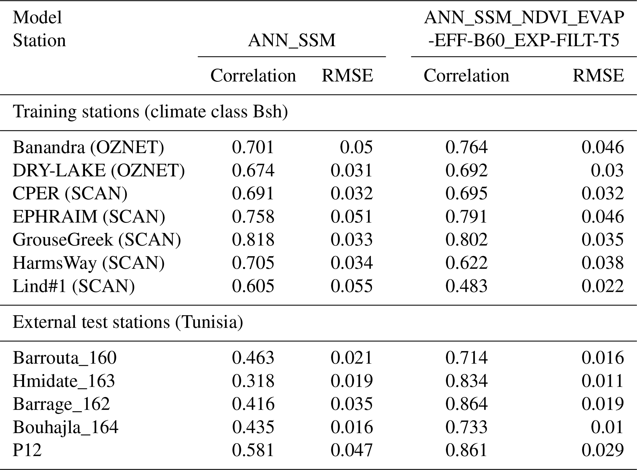
However, the consideration of additional features, namely, the NDVI, evaporation efficiency and SWI in the ANN models, resulted in good agreement between the in situ and predicted RZSM values (Fig. 4). The correlation values were improved by 60.04 %, 169.5 %, 112.02 %, 80.23 % and 53.7 % at stations Barrouta-160, Hmidate_163, Barrage_162, Bouhajla_164 and P12, respectively, with the ANN_SSM_NDVI_EVAP-EFF-B60_EXP-FILT-T5 model over ANN_SSM model values. Similarly, RMSE values were reduced (Table 5). As shown in Fig. 4, the most complex ANN model is able to capture the variations of RZSM. This finding highlights the added value of our hybrid approach based on an association of a machine learning method with process-related variables. Instead of injecting uncertain information into physical models, such as soil properties, we used a nonparametric method related to physical processes without using forcing data that may be subject to errors and potentially lead to inaccurate tracking of the long-term evolution of soil moisture.
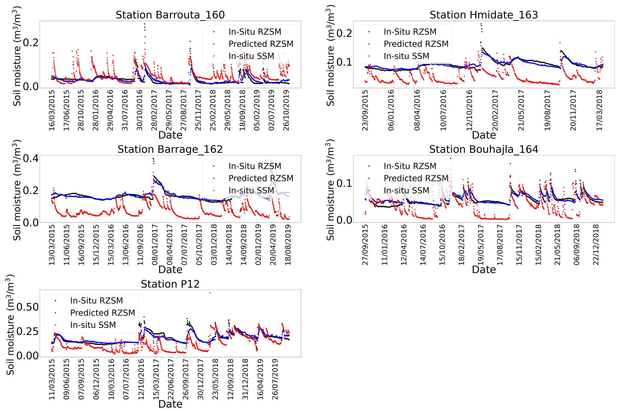
Figure 4In situ SSM, in situ RZSM, and predicted RZSM series at the stations in the Kairouan Plain (Tunisia) with model ANN_SSM_NDVI_EVAP-EFF-B60_EXP-FILT-T5 (see Appendix G for a larger figure format).
A second comparison can be conducted between the quality of fit of these independent datasets and training datasets. Actually, the climate class of the Tunisian stations is Bsh (see Appendix A). At the training stage, no station falls into climate class Bsh (see Appendix A). However, some training stations fall under a similar climate class, which is Bsk (see Appendix B). Table 5 presents correlation and RMSE values for these training stations and Tunisian sites with both models ANN_SSM and ANN_SSM_NDVI_EVAP-EFF-B60_EXP-FILT-T5. For all training stations, performance metrics are slightly enhanced, with the most complex ANN model compared to the reference model ANN_SSM, except for stations GrouseCreek, Harmsway and Lind#1, whose performance decreases. Overall, the range of correlation values is similar for training and external validation stations with model ANN_SSM_NDVI_EVAP-EFF-B60_EXP-FILT-T5, and RMSE is greatly reduced for the Tunisian stations compared to the training stations. Given the results on unseen datasets, namely, on Tunisia, the performance of the most complex ANN model is good as it is able to generalize the patterns present in the training dataset.
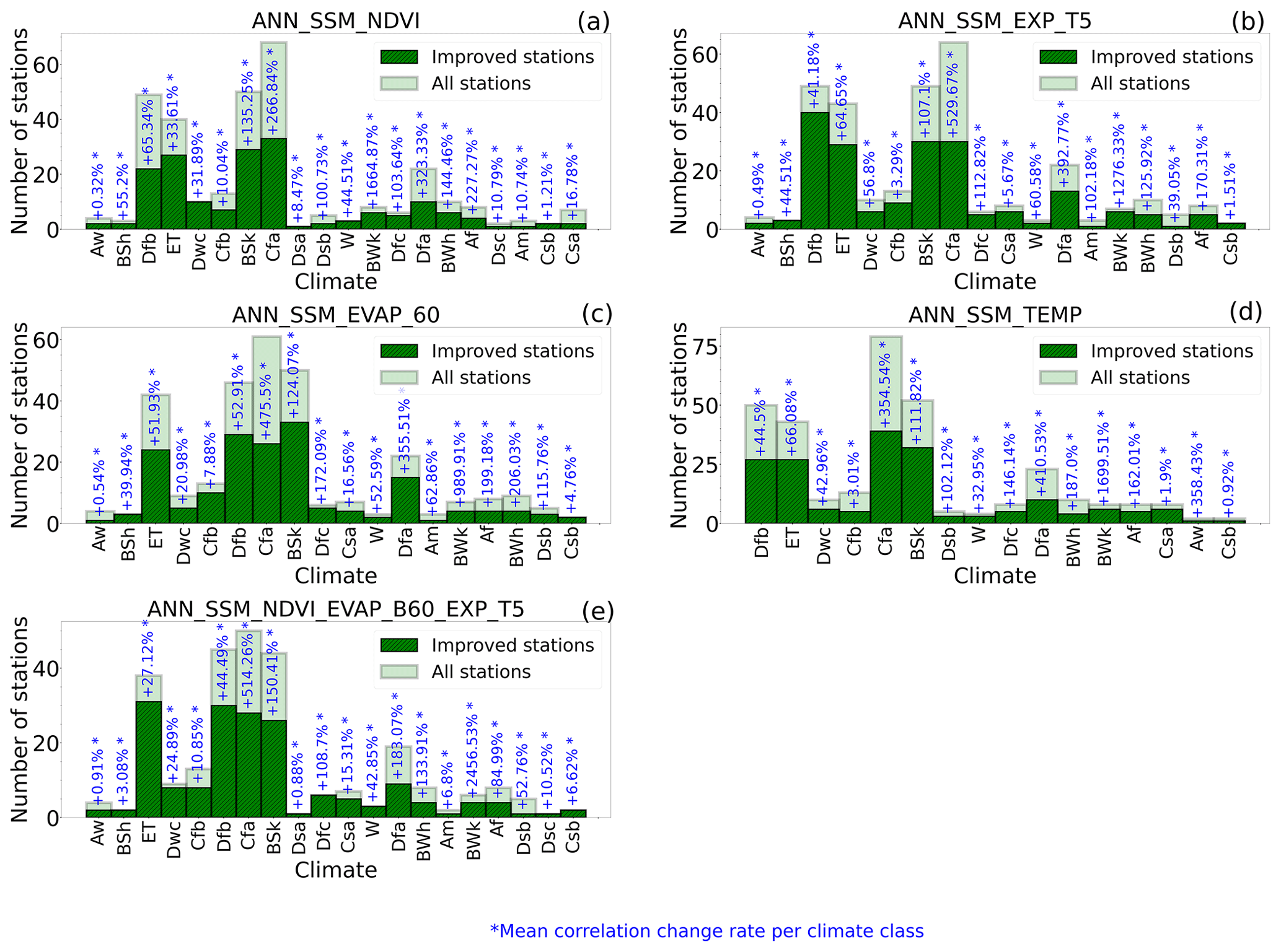
Figure 5Climate classification of the stations performing better with models (a) ANN_SSM_NDVI, (b) ANN_SSM_EXP-FILT-T5, (c) ANN_SSM_EVAP-EFF-B60, (d) ANN_SSM_TEMP and (e) ANN_SSM_NDVI_EVAP-EFF-B60_EXP-FILT-T5 compared to model ANN_SSM (dark green corresponds to stations whose correlation improved with complexified models, light green corresponds to total stations and rate in blue corresponds to the mean correlation change rate per climate class).
Table 6Performance metrics of models ANN_SSM, ANN_SSM_NDVI and ANN_SSM_NDVI_EVAP-EFF-B60_EXP-FILT-T5 at the sites in southern India and northern Italy.
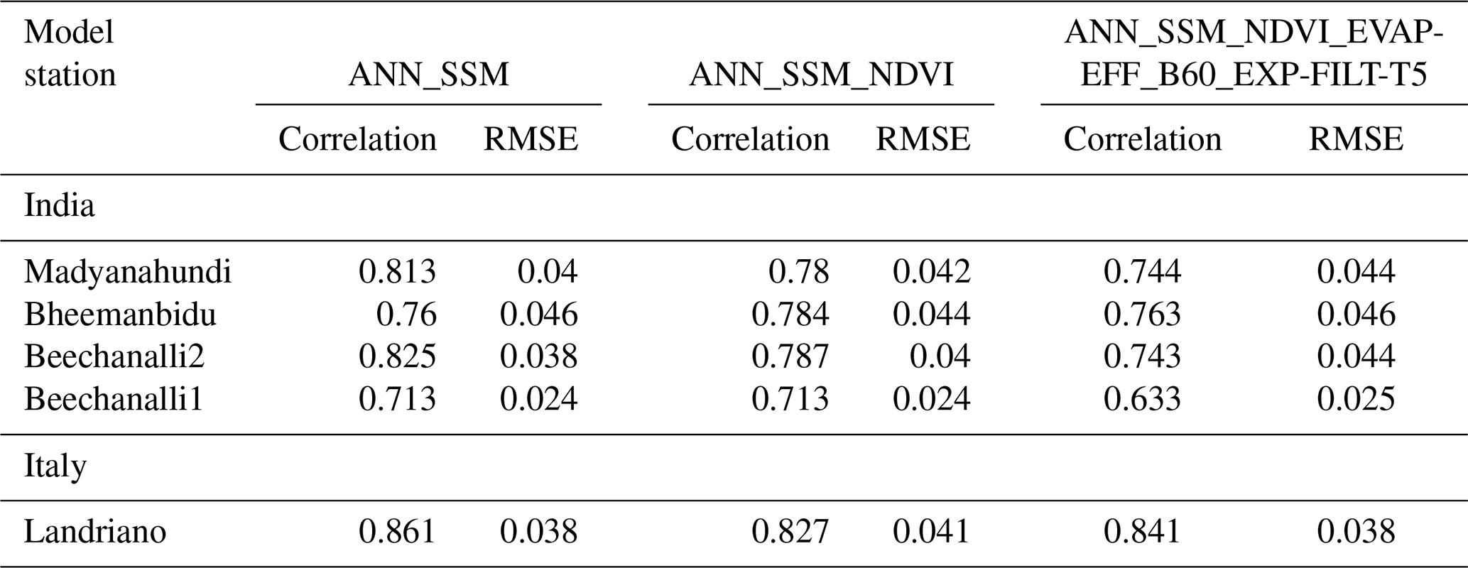
At the southern Indian stations, the ANN_SSM model yielded good agreement even without the integration of process-related features (Table 6). These features added little to nonsignificant improvement. The same observation was made at the Italian site. The application of multiple features performed the best under arid conditions, e.g., in Tunisia. In the tropical and temperate climate regions, this was not the case. The presence of clouds in the MODIS NDVI and potential evapotranspiration products could explain this observation at sites of southern India and northern Italy. In southern India, for instance, the maximum variability in soil moisture occurred during the monsoon season, which is characterized by a large amount of clouds. Moreover, the coarse resolution of the MODIS NDVI product makes it sometimes not adapted to the considered site. Chen et al. (2016) investigated the impact of sample impurity and landscape heterogeneity on crop classification using coarse-spatial-resolution MODIS imagery. They showed that the sample impurity such as mixed crop types in a specific sample, compositional landscape heterogeneity, which is the richness and evenness of land cover types in a landscape, and configurational heterogeneity, which is the complexity of the spatial structure of land cover types in a specific landscape, are sources of uncertainty affecting crop area mapping when using coarse-spatial-resolution imagery. High-resolution NDVI from sensors like Sentinel-2 could have been used in this exercise to mitigate the spatial resolution issue; however, MODIS data were privileged in order to provide NDVI and PET from the same sensor.
Climate analysis of the results yielded by the different models indicated that, among all the models, the climate class with the highest mean correlation change rate (Fig. 5) was class BWk (see Appendix A), which regroups desert areas where the link between SSM and RZSM is weak due to high evaporative rates. Class Dfa (see Appendix A), which includes areas experiencing harsh and cold winters, also yielded a high mean correlation change rate (>100 %). Similarly, at stations of this climate type, the link between the surface and root zone is poor. In regard to class Cfa (see Appendix A), in which more than 80 % of the total stations belong to the SCAN network, the high mean correlation change rate could be explained by the surface–subsurface decoupling phenomena detected within this network, as previously reported in Souissi et al. (2020). The model with the largest number of stations with improved predictions over the ANN_SSM model predictions was ANN_SSM_NDVI_EVAP-EFF-B60_EXP-FILT-T5. Actually, the coupled use of process-related features in the ANN models exerted a greater impact on the prediction accuracy than that exerted by the one-at-a-time application of these features. In model ANN_SSM_NDVI_EVAP-EFF-B60_EXP-FILT-T5, the three process-based features jointly employed seemed to counterbalance the weight of the three SSM features. In this model, the process-related features were equally represented versus the SSM information depicted by three features. The redundancy of the considered SSM information could explain the limited impact of the one-at-a-time addition of process-related features.
In addition, Karthikeyan and Mishra (2021) demonstrated that, at root depths beyond 20 cm, the importance of SSM was notably lower than that at the 20 cm depth, signifying decorrelation between surface and deeper SM values, which is in accordance with the findings in Souissi et al. (2020), and it was further revealed that vegetation exhibits a higher importance than that of the meteorological predictors and precipitation. Kornelsen and Coulibaly (2014) indicated that evapotranspiration is the most important meteorological input for the prediction of soil moisture in the root zone with the MLP, which reflects the importance of the water vapor flux in soil moisture state determination.
where X denotes a process-related variable (X ∈ [“NDVI”, “EXP-FILT-T5”, “EVAP-EFF-B60”, “TEMP”]).
The world map illustrated in Fig. 6 shows the best-performing ANN models based on the mean correlation change rate (Eq. 5). We assumed that the results in a given area of a specific climate class could be extended to other areas of the same climate class even if we did not consider the data for these areas. The climate classes without at least one station were marked in black and labeled with “NO DATA”.
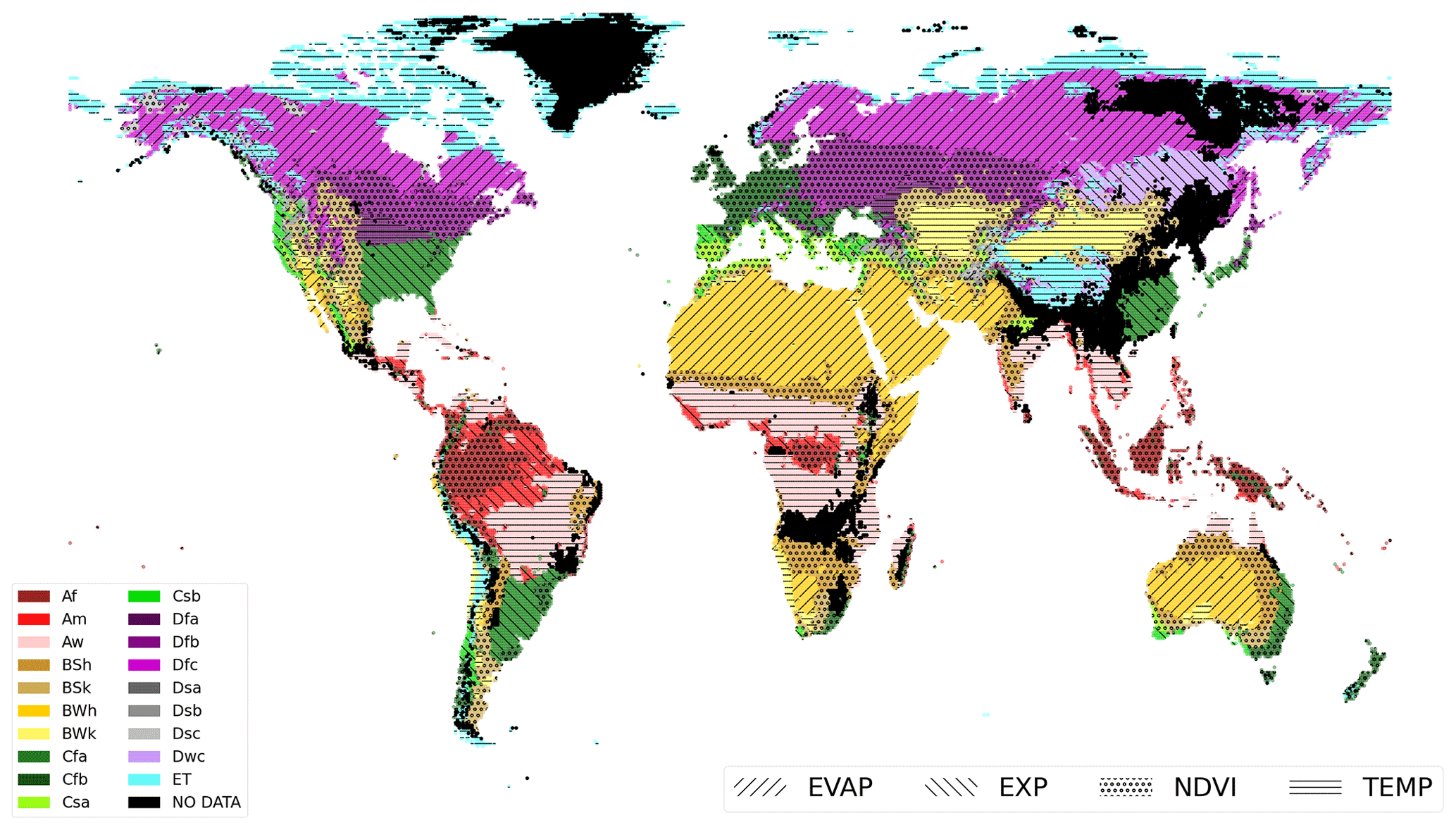
Figure 6World map of the best-performing ANN models per climate class based on the mean correlation change rate; colors correspond to climate classes (see Appendix A), and hatches correspond to the most contributive input to the predictions, namely, EVAP (evaporation efficiency), EXP (exponential filter SWI), NDVI, and TEMP (surface soil temperature).
In arid areas such as the eastern and western sides of the USA with high evaporation rates, ANN_SSM_EVAP-EFF-B60 was the best-performing model. Similarly, in bare areas of Africa, the Middle East and Australia where the Bwh climate class prevailed (arid desert hot climate; see Appendix A), the evaporation efficiency was the best informative variable.
In the internal part of continental Europe and near the Mediterranean basin, the NDVI was the most relevant indicator for RZSM estimation, where agricultural fields dominated. Similarly, the Great Plains region in the USA was deeply affected by the NDVI, as this region is a cultivated area. In Nordic areas characterized by the ET climate class (Polar Tundra climate, see Appendix A) and mainly covered by grassland and shrubland areas according to ESA CCI land cover maps.
In Nordic areas characterized by the ET climate class, the soil temperature was the most important root-zone soil moisture indicator, mainly because of the freeze–thaw events encountered in these regions. In tropical savannah wet areas (class Aw; see Appendix A), the ANN_SSM_TEMP model was the best-performing model.
This classification definitely suffered from limitations mainly provoked by the generalization of the climatic analysis results to areas not considered in this study. For instance, in regions of climate class Dfc (cold dry without a dry season, cold summer climate; see Appendix A), we expect the temperature to serve as the most relevant indicator instead of the evaporation efficiency.
In this study, we developed several ANN models to estimate RZSM based either solely on in situ SSM information or on a group of process-related features in addition to SSM, namely, the soil water index computed with a recursive exponential filter, evaporation efficiency, NDVI and surface soil temperature. Different regions across the globe with distinct land cover and climate patterns were considered. The main conclusion of this study was that the consideration of more features in addition to SSM information could enhance the accuracy of RZSM predictions mainly in regions where the link between SSM and RZSM is weak.
In arid areas with high evaporation rates, the most informative feature was the evaporation efficiency. In regions with agricultural fields, the NDVI was, for example, the most relevant indicator to predict RZSM. Overall, the best-performing model included the surface soil moisture, NDVI, SWI and evaporation efficiency as features. The robustness of the approach was further assessed through additional tests considering external sites in central Tunisia, India and Italy. Similarly, the process-related features exerted a positive impact on the prediction accuracy when combined with surface soil moisture in the case of Tunisia. The mean correlation across the five Tunisian stations sharply increased from 0.44 when only SSM was considered to 0.8 when all process-related features were combined with SSM. In India and Italy, the correlations were already high with the reference model ANN_SSM. The change in correlation after the addition of process-related features, namely, NDVI, is about −0.04, which is nonsignificant and is potentially because of the cloudy conditions in India and the noisy MODIS products. Also, the crop heterogeneity and sample impurity make MODIS NDVI products not adapted to all sites.
As a research perspective, datasets can be separated into clusters corresponding to major climate classes and/or soil types. More analysis can be conducted in this direction to eventually make connections between the different inputs and climate/soil configurations.
Future work will examine the ability of the developed model to estimate RZSM across larger areas based on remote-sensing global soil moisture products. The use of remote-sensing-derived soil moisture products may yield lower correlations with the reference model ANN_SSM, which potentially implies further improvement when process-related features are added.
| Af | Tropical rainforest |
| Am | Tropical monsoon |
| As | Tropical savanna dry |
| Aw | Tropical savanna wet |
| BWk | Arid desert cold |
| BWh | Arid desert hot |
| BWn | Arid desert with frequent fog |
| BSk | Arid steppe cold |
| BSh | Arid steppe hot |
| BSn | Arid steppe with frequent fog |
| Csa | Temperate dry hot summer |
| Csb | Temperate dry warm summer |
| Csc | Temperate dry cold summer |
| Cwa | Temperate dry winter, hot summer |
| Cwb | Temperate dry winter, warm summer |
| Cwc | Temperate dry winter, cold summer |
| Cfa | Temperate without a dry season, hot summer |
| Cfb | Temperate without a dry season, warm summer |
| Cfc | Temperate without a dry season, cold summer |
| Dsa | Cold dry summer, hot summer |
| Dsb | Cold dry summer, warm summer |
| Dsc | Cold dry summer, cold summer |
| Dsd | Cold dry summer, very cold winter |
| Dwa | Cold dry winter, hot summer |
| Dwb | Cold dry winter, warm summer |
| Dwc | Cold dry winter, cold summer |
| Dwd | Cold dry winter, very cold winter |
| Dfa | Cold dry without a dry season, hot summer |
| Dfb | Cold dry without a dry season, warm summer |
| Dfc | Cold dry without a dry season, cold summer |
| Dfd | Cold dry without a dry season, very cold winter |
| ET | Polar tundra |
| EF | Polar eternal winter |
| W | Water |
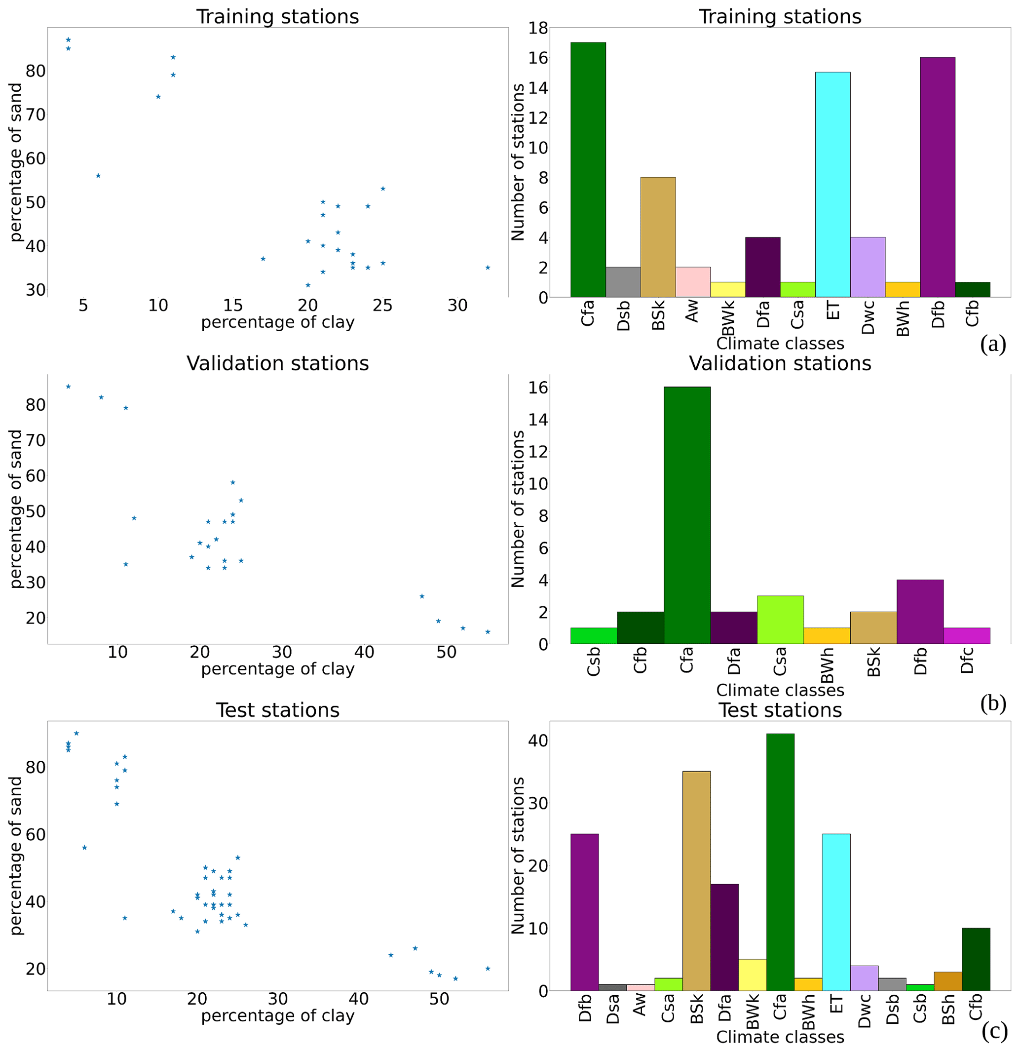
Figure B1Climate and soil texture for (a) training stations, (b) validation stations and (c) test stations.
Evaporation efficiency (Sect. 2.2.2): the standard equations to compute evaporation efficiency (β3) in Merlin et al. (2010) are as follows:
where θL is the water content in the soil layer of thickness L. P is a parameter computed as follows:
θmax is the soil moisture at saturation. LEp is the potential evaporation. L1 is the thinnest represented soil layer, and A3 (unitless) and B3 (W m−2) are the two best-fit parameters a priori depending on the soil texture and structure, respectively.
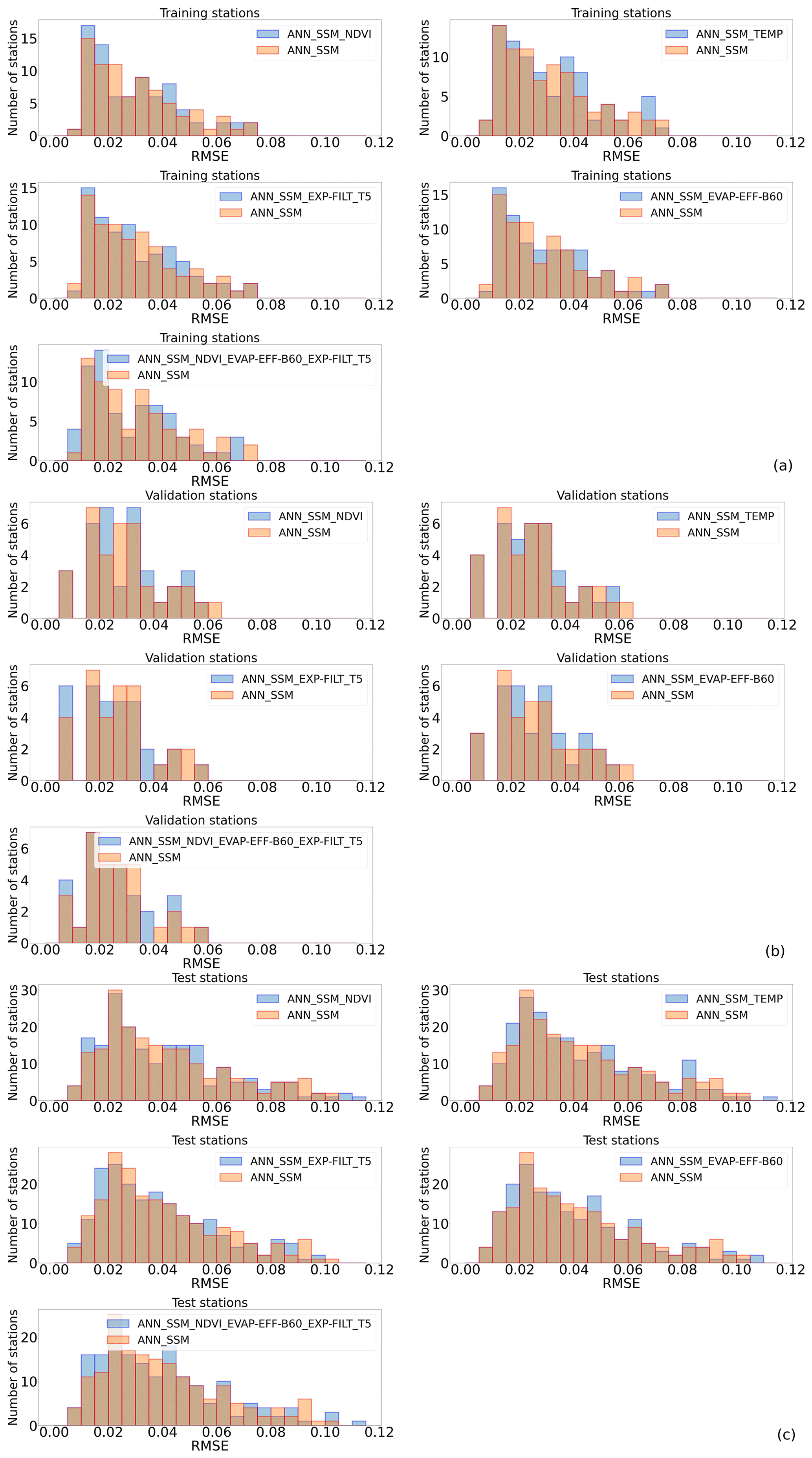
Figure D1RMSE histograms of all tested ANN models compared to ANN_SSM (a) on training stations, (b) on validation stations and (c) on test stations.
E1 Training stations
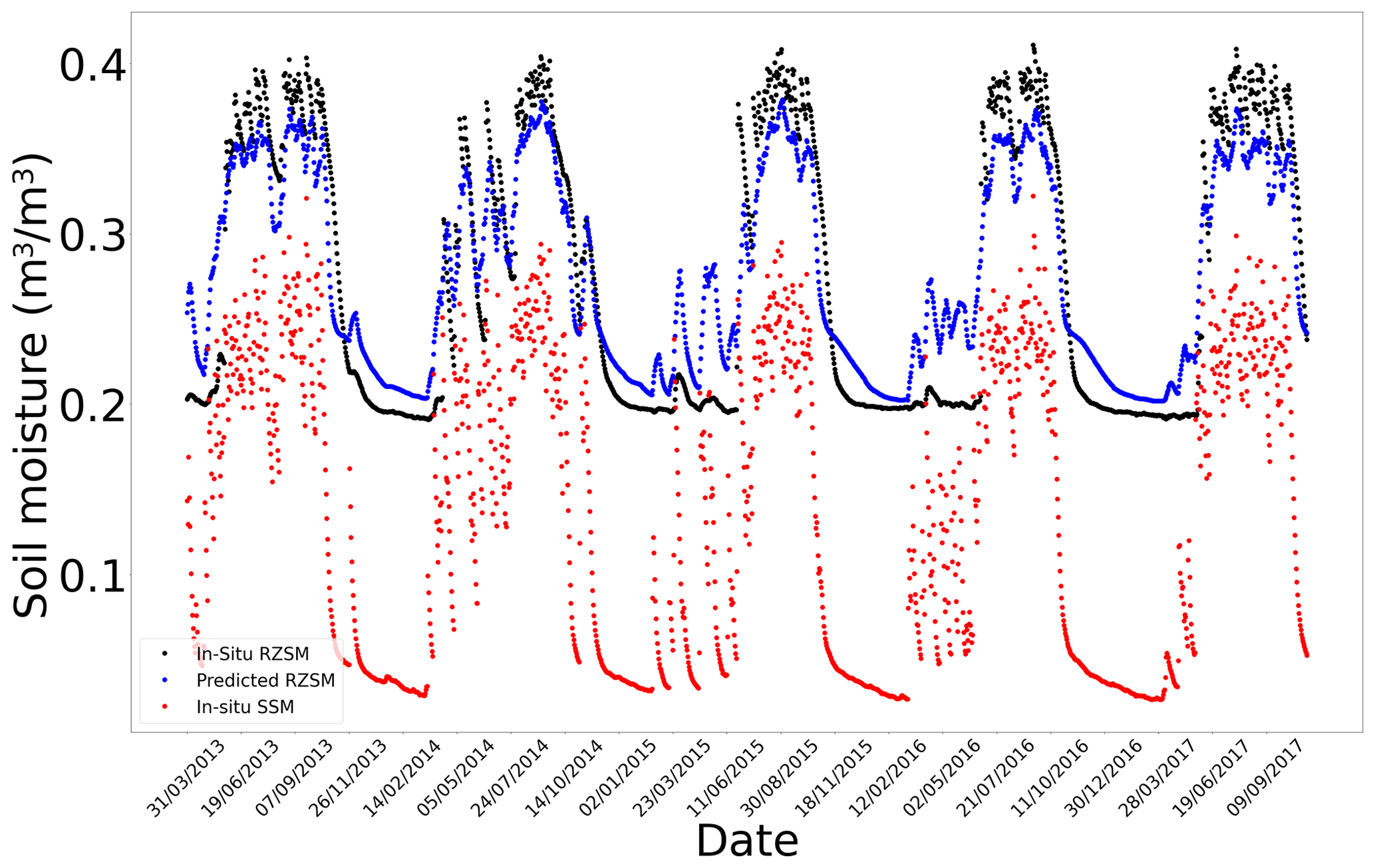
Figure E1In situ SSM, in situ RZSM, and predicted RZSM series at station Beloufoungou Mid (AMMA-CATCH) with model ANN_SSM.
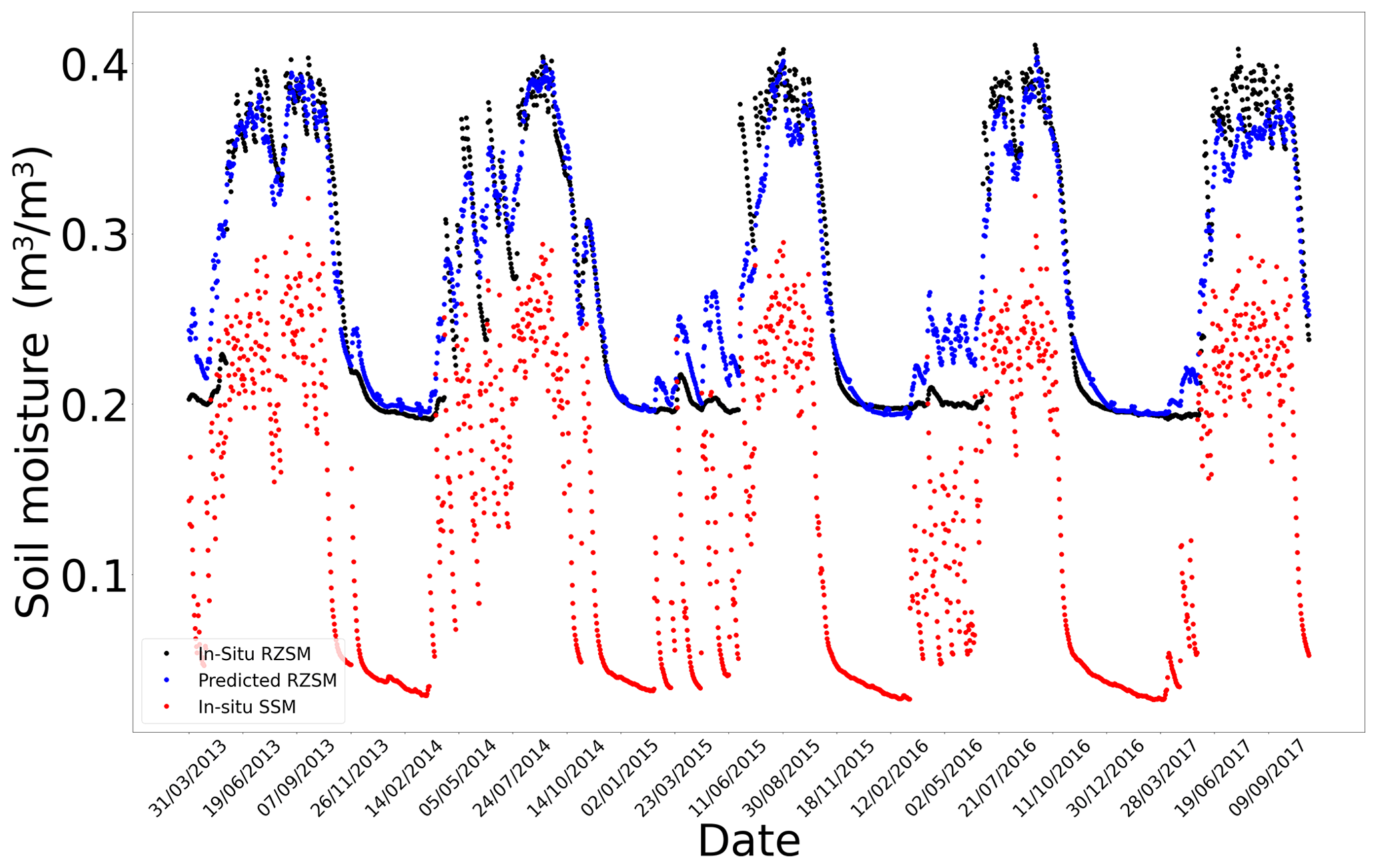
Figure E2In situ SSM, in situ RZSM, and predicted RZSM series at station Beloufoungou Mid (AMMA-CATCH) with model ANN_SSM_NDVI_EVAP-EFF-B60_EXP-FILT-T5.
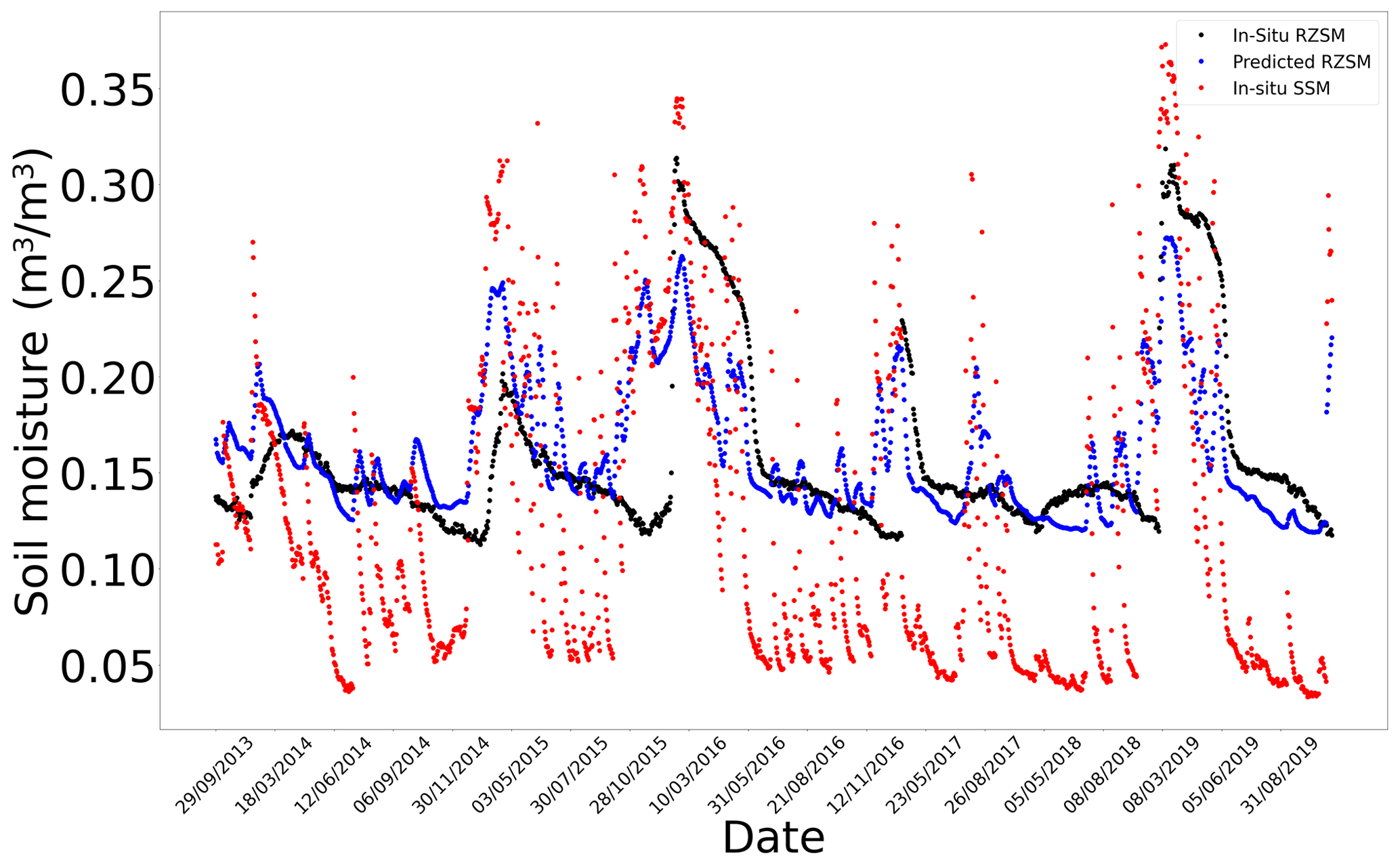
Figure E3In situ SSM, in situ RZSM, and predicted RZSM series at station HarmsWay (SCAN) with model ANN_SSM.

Figure E4In situ SSM, in situ RZSM, and predicted RZSM series at station HarmsWay (SCAN) with model ANN_SSM_NDVI_EVAP-EFF-B60_EXP-FILT-T5.
E2 Validation stations
Figure E5In situ SSM, in situ RZSM, and predicted RZSM series at station Cabrieres D'Avignon (SMOSMANIA) with model ANN_SSM.

Figure E6In situ SSM, in situ RZSM, and predicted RZSM series at station Cabrieres D'Avignon (SMOSMANIA) with model ANN_SSM_NDVI_EVAP-EFF-B60_EXP-FILT-T5.
Figure E7In situ SSM, in situ RZSM, and predicted RZSM series at station Nephi (SCAN) with model ANN_SSM.
Figure E8In situ SSM, in situ RZSM, and predicted RZSM series at station Nephi (SCAN) with model ANN_SSM_NDVI_EVAP-EFF-B60_EXP-FILT-T5.
E3 ISMN test stations
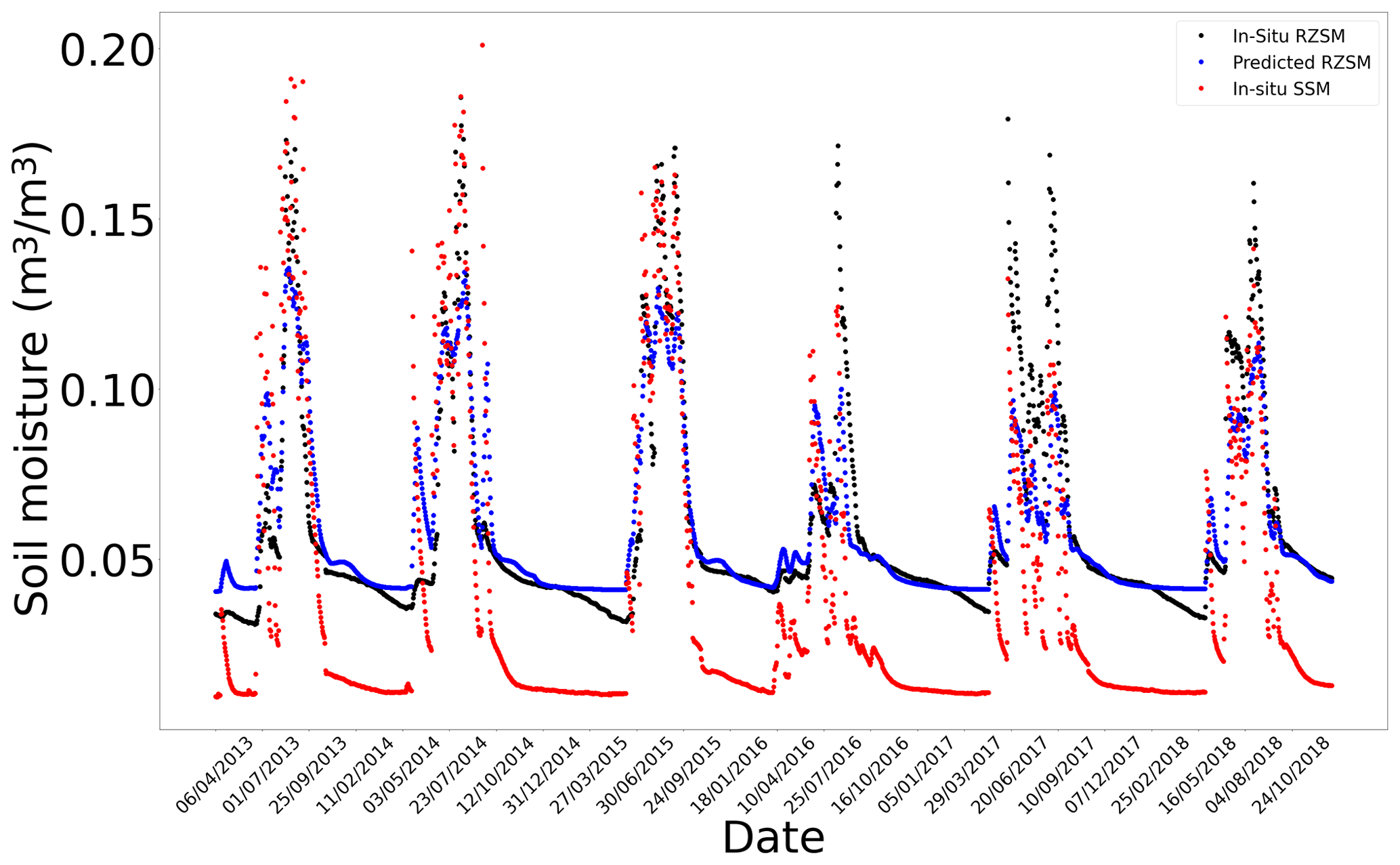
Figure E9In situ SSM, in situ RZSM, and predicted RZSM series at station Wankama (AMMA-CATCH) with model ANN_SSM.
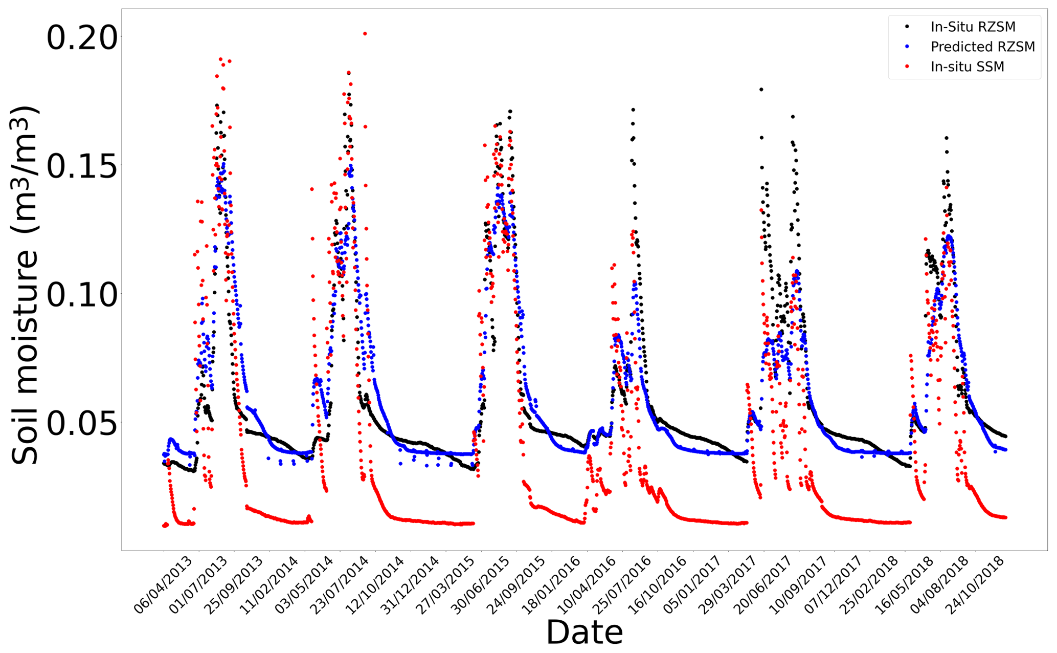
Figure E10In situ SSM, in situ RZSM, and predicted RZSM series at station Wankama (AMMA-CATCH) with model ANN_SSM_NDVI_EVAP-EFF-B60_EXP-FILT-T5.
Figure E11In situ SSM, in situ RZSM, and predicted RZSM series at station 2.04 (HOBE) with model ANN_SSM.
Figure E12In situ SSM, in situ RZSM, and predicted RZSM series at station 2.04 (HOBE) with model ANN_SSM_ NDVI_EVAP-EFF-B60_EXP-FILT-T5.

Figure F1In situ SSM, in situ RZSM, and predicted RZSM series at station Lind#1 with model ANN_SSM.
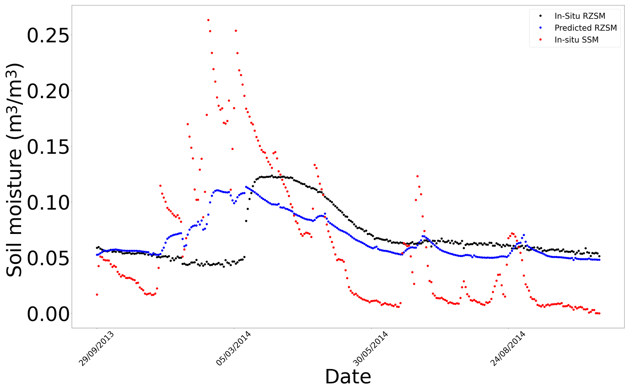
Figure F2In situ SSM, in situ RZSM, and predicted RZSM series at station Lind#1 with model ANN_SSM_NDVI_EVAP-EFF-B60_EXP-FILT-T5.

Figure F3In situ SSM, in situ RZSM, and predicted RZSM series at station PineNut with model ANN_SSM.
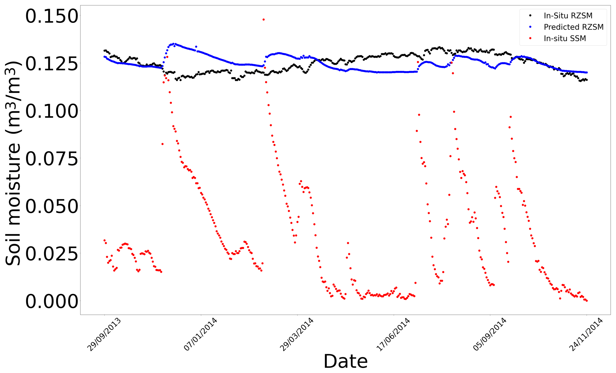
Figure F4In situ SSM, in situ RZSM, and predicted RZSM time series at the stations in the Kairouan Plain (Tunisia) with model ANN_SSM_NDVI_EVAP-EFF-B60_EXP-FILT-T5 (see Appendix G for a larger figure format).

Figure F5In situ SSM, in situ RZSM, and predicted RZSM series at station S-Coleambally with model ANN_SSM.
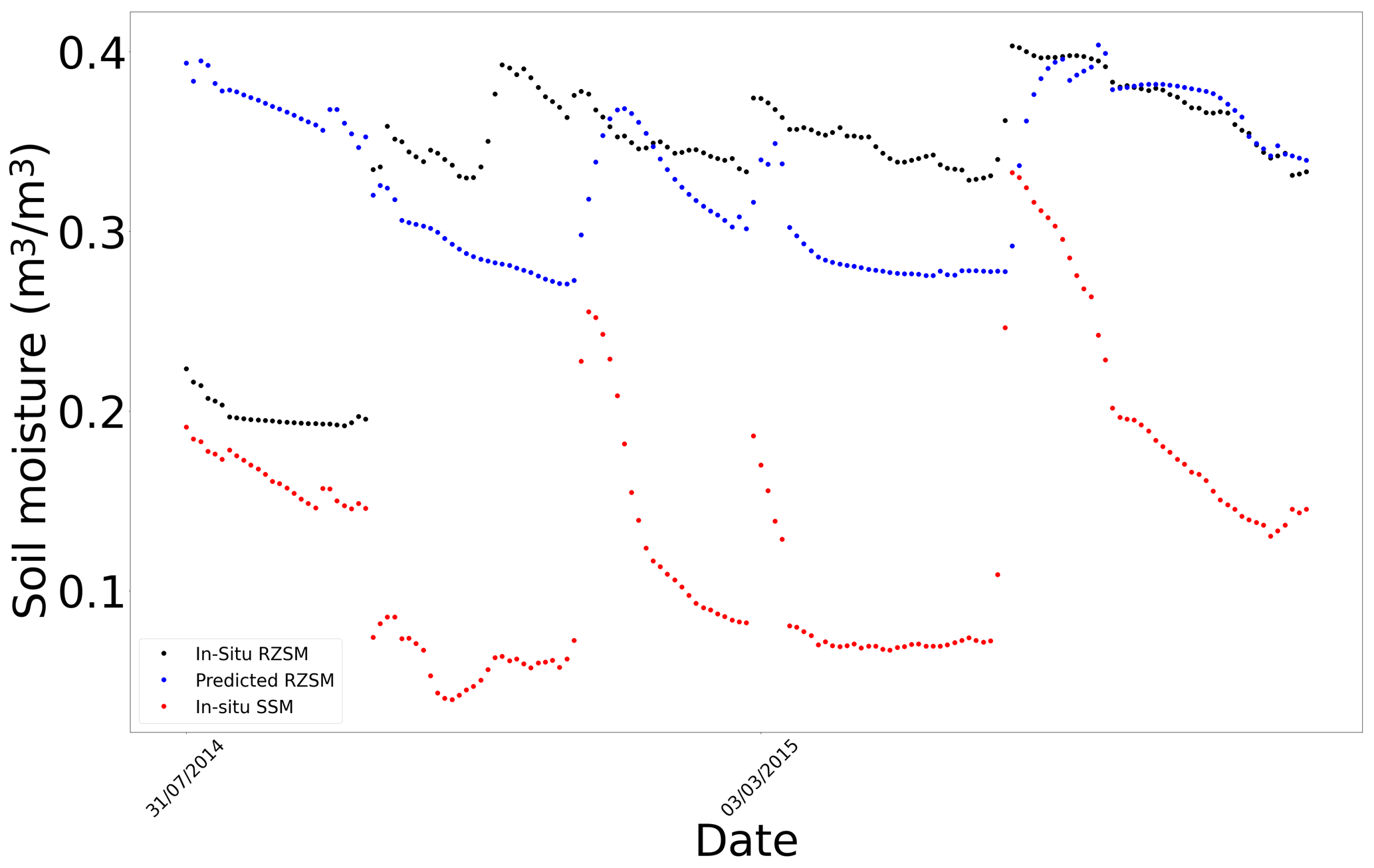
Figure F6In situ SSM, in situ RZSM, and predicted RZSM series at station S-Coleambally with model ANN_SSM_NDVI_EVAP-EFF-B60_EXP-FILT-T5.
Figure F7In situ SSM, in situ RZSM, and predicted RZSM series at station Widgiewa with model ANN_SSM.
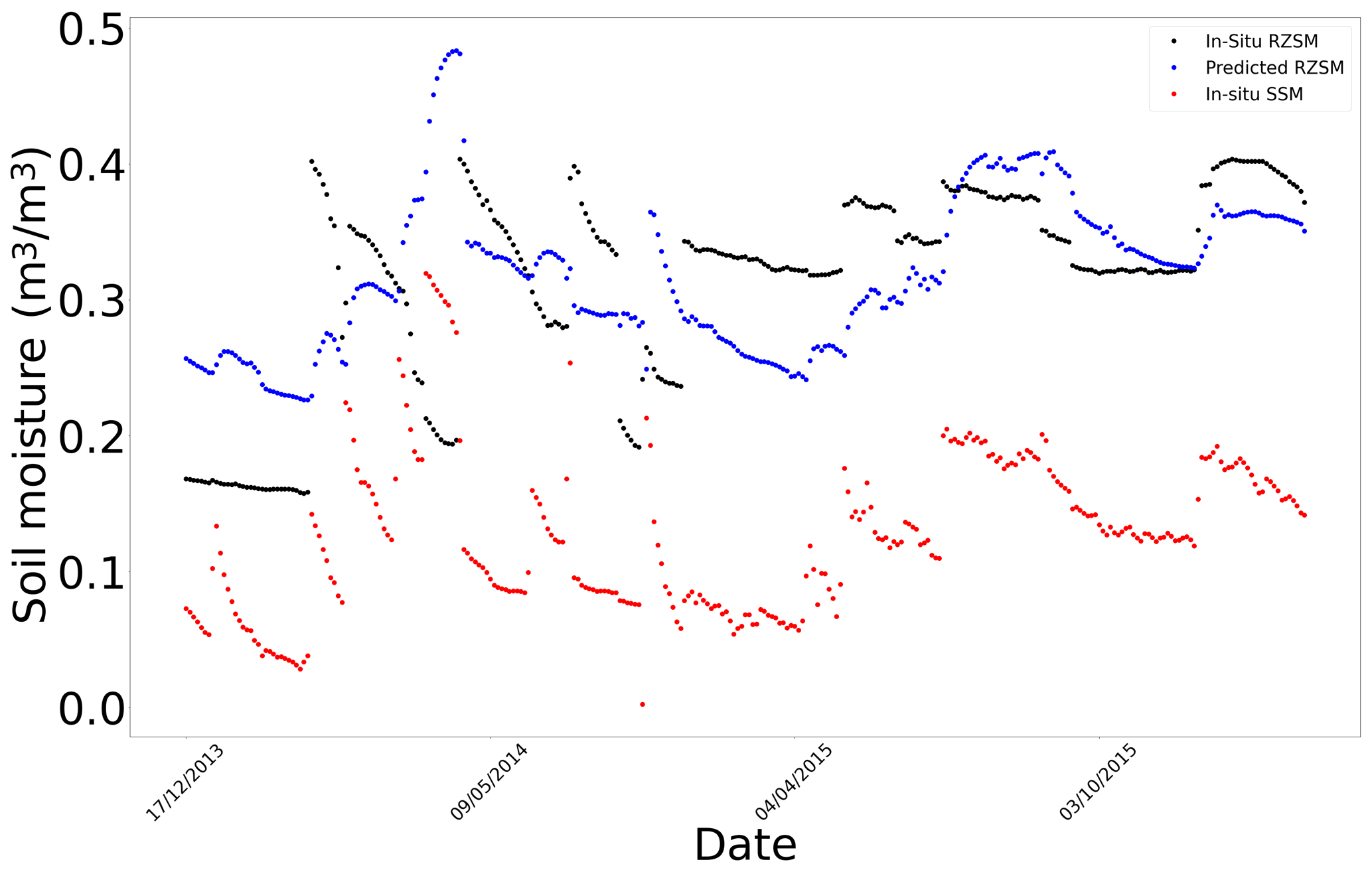
Figure F8In situ SSM, in situ RZSM, and predicted RZSM series at station Widgiewa with model ANN_SSM_NDVI_EVAP-EFF-B60_EXP-FILT-T5.
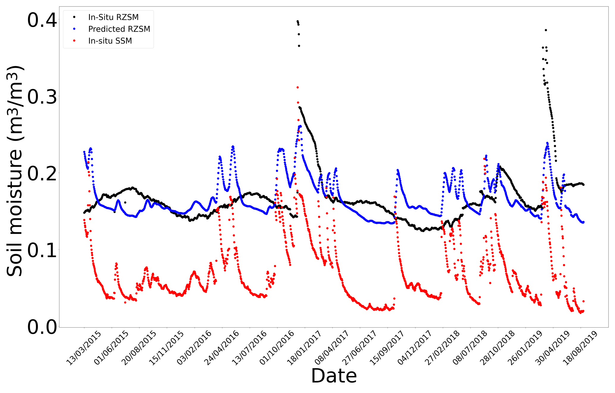
Figure G1In situ SSM, in situ RZSM, and predicted RZSM series at station Barrage-162 (Tunisia) with model ANN_SSM.
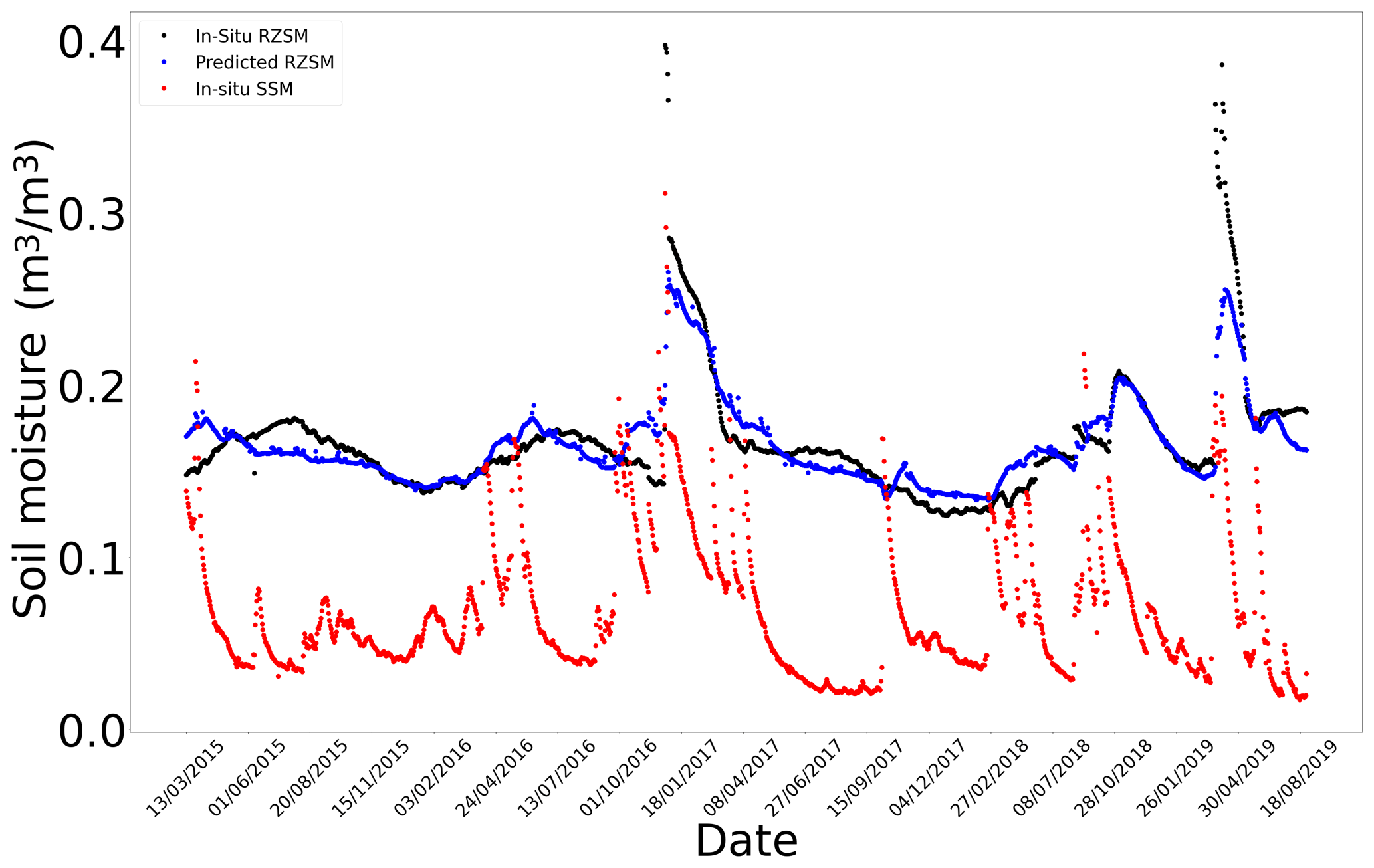
Figure G2In situ SSM, in situ RZSM, and predicted RZSM series at station Barrage-162 (Tunisia) with model ANN_SSM_NDVI_EVAP-EFF-B60_EXP-FILT-T5.
Figure G3In situ SSM, in situ RZSM, and predicted RZSM series at station Barrouta_160 (Tunisia) with model ANN_SSM.
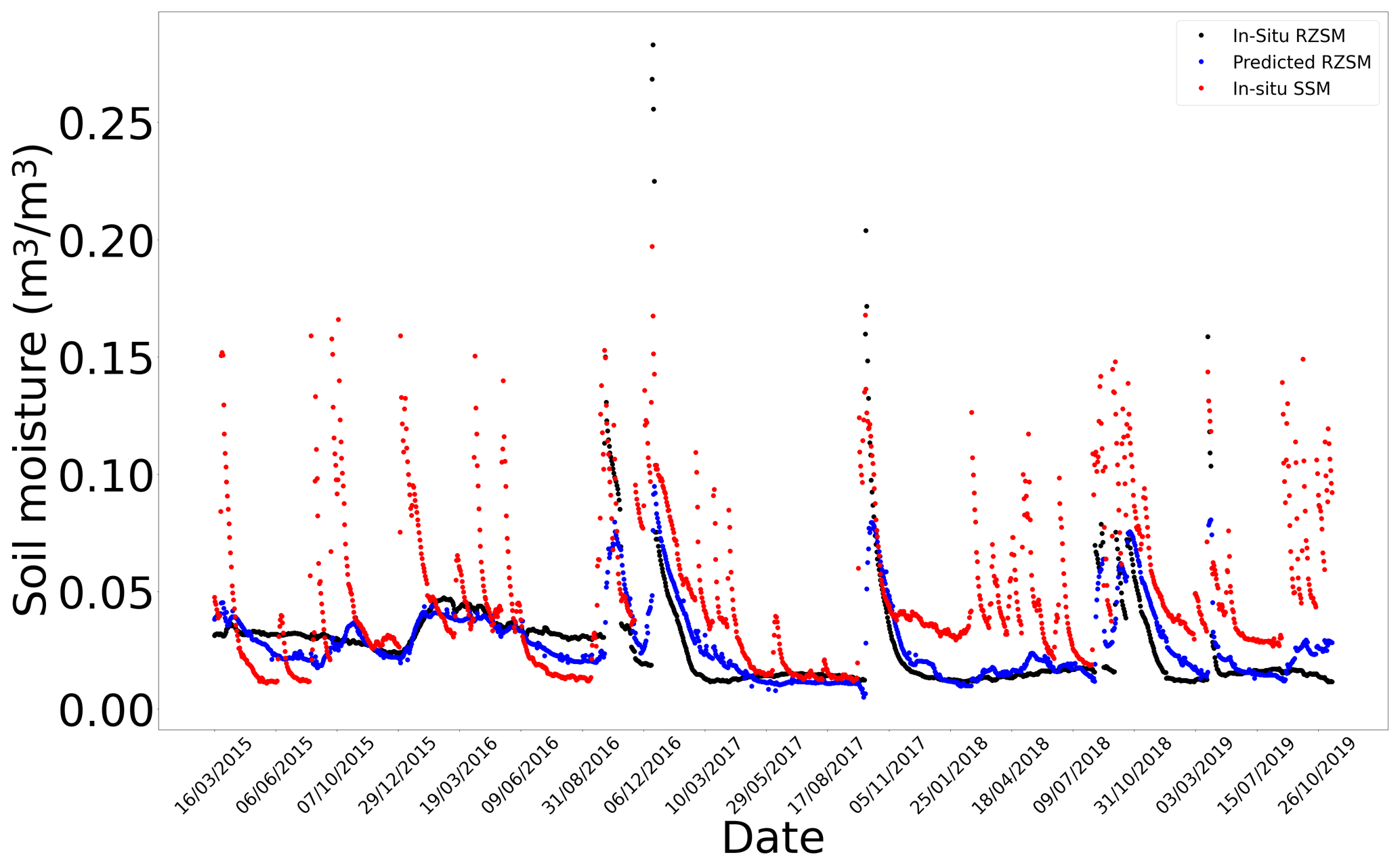
Figure G4In situ SSM, in situ RZSM, and predicted RZSM series at station Barrouta_160 (Tunisia) with model ANN_SSM_NDVI_EVAP-EFF-B60_EXP-FILT-T5.
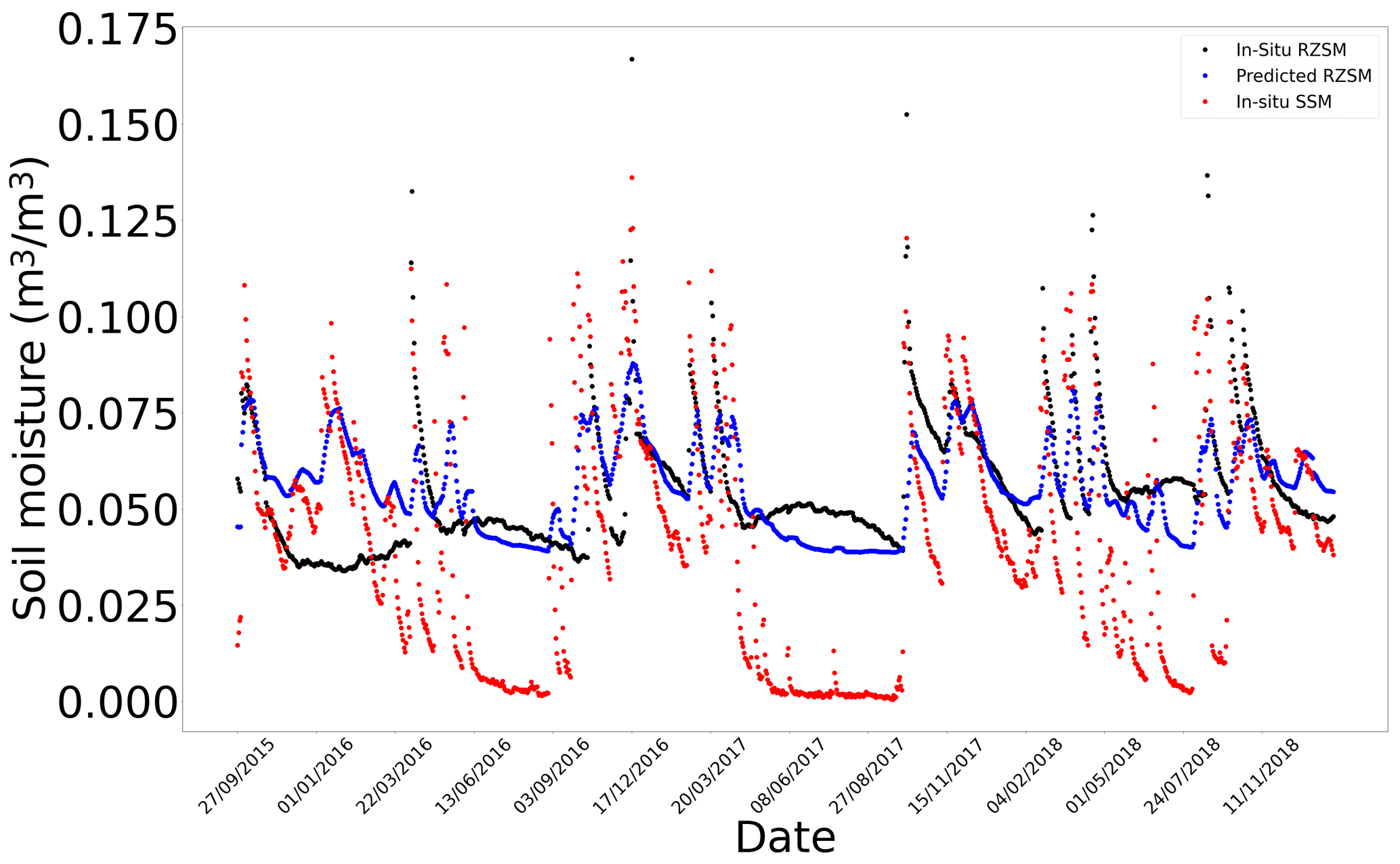
Figure G5In situ SSM, in situ RZSM, and predicted RZSM series at station Bouhajla_164 (Tunisia) with model ANN_SSM.
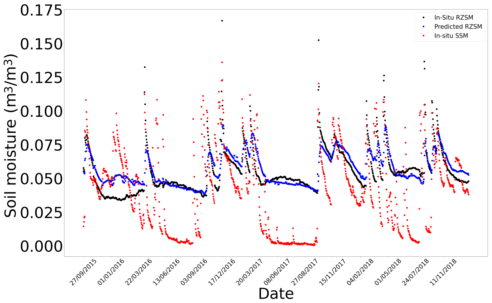
Figure G6In situ SSM, in situ RZSM, and predicted RZSM series at station Bouhajla_164 (Tunisia) with model ANN_SSM_NDVI_EVAP-EFF-B60_EXP-FILT-T5.
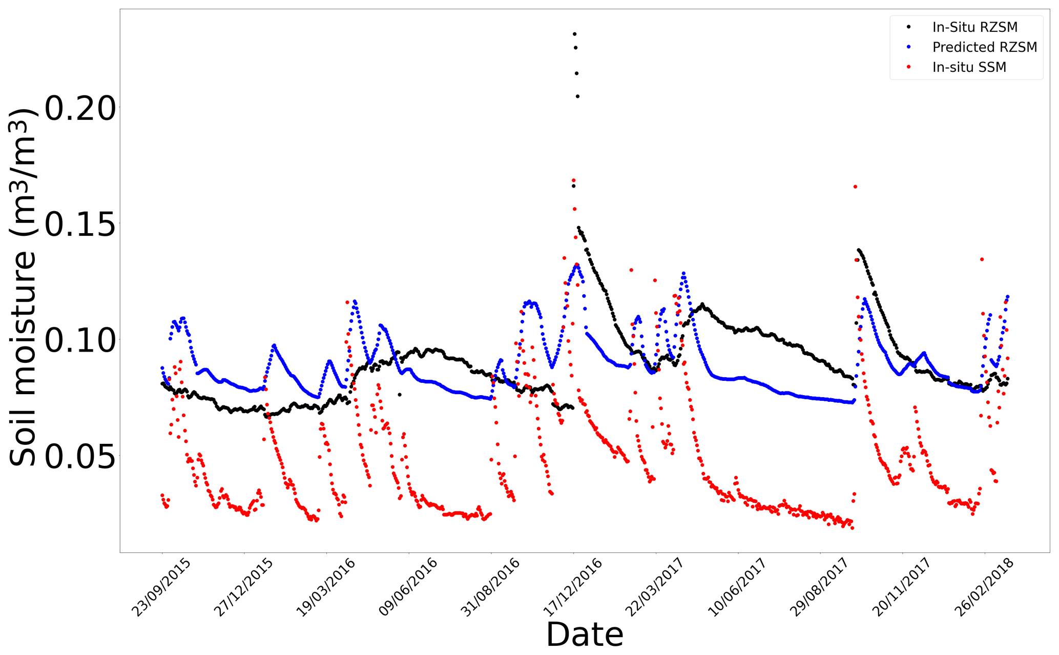
Figure G7In situ SSM, in situ RZSM, and predicted RZSM series at station Hmidate_163 (Tunisia) with model ANN_SSM.
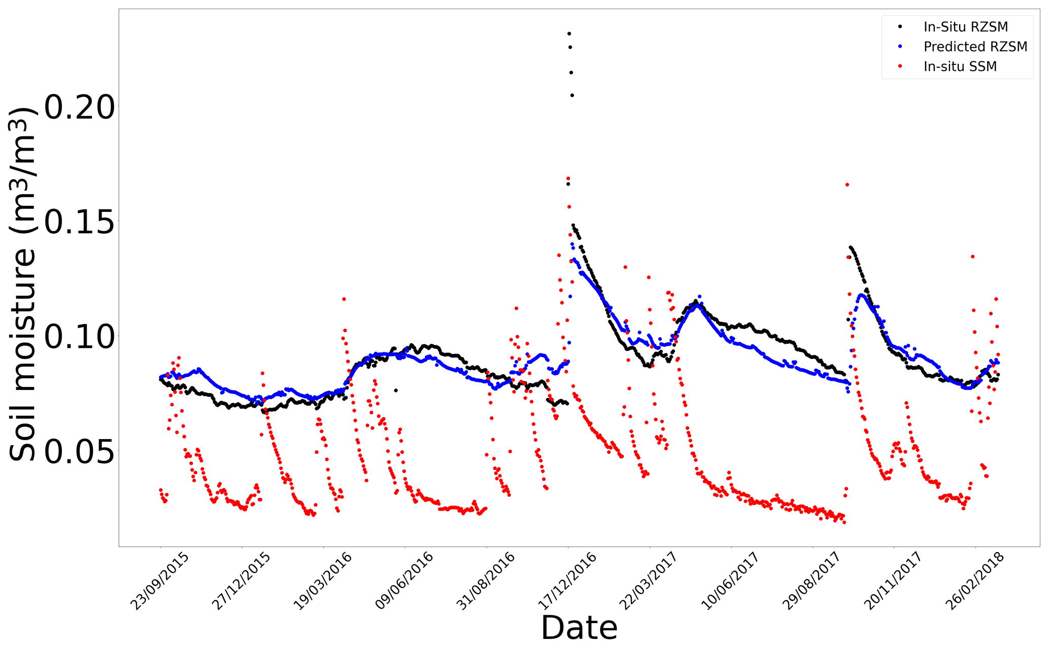
Figure G8In situ SSM, in situ RZSM, and predicted RZSM series at station Hmidate_163 (Tunisia) with model ANN_SSM_NDVI_EVAP-EFF-B60_EXP-FILT-T5.

Figure G9In situ SSM, in situ RZSM, and predicted RZSM series at station P12 (Tunisia) with model ANN_SSM.
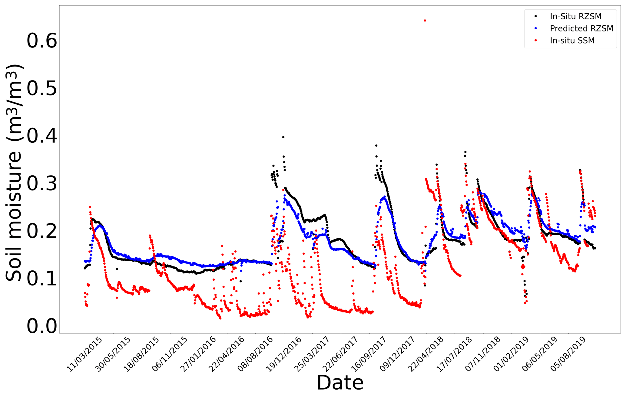
Figure G10In situ SSM, in situ RZSM, and predicted RZSM series at station P12 (Tunisia) with model ANN_SSM_NDVI_EVAP-EFF-B60_EXP-FILT-T.
The code is not publicly accessible because this is in the requirements of some projects.
In situ soil moisture data and in situ surface temperature data can be publicly accessed from the International Soil moisture data hosting facility (Dorigo et al.,2021). MODIS NDVI data are available at https://doi.org/10.5067/MODIS/MOD13Q1.006 (Didan, 2015) and MODIS potential evapotranspiration data are available at https://doi.org/10.5067/MODIS/MOD16A3.006 (Running et al., 2017).
The methodology was established by AAB, RS and MZ. The original draft was written by RS. The manuscript was reviewed and edited by all the authors. Soil moisture data over the Italian site and the site description were provided by CC and MM. Soil moisture data over the Indian site and the site description were provided by SM, SKM and DBU. This PhD thesis is under the supervision of MZ and AAB. All the authors have read and agreed to the published version of the manuscript.
The contact author has declared that neither they nor their co-authors have any competing interests.
Publisher's note: Copernicus Publications remains neutral with regard to jurisdictional claims in published maps and institutional affiliations.
The authors were financially supported by the French National Research Agency (ANR) and the French National Space Agency (CNES) for this PhD thesis. The authors also thank the International Soil Moisture Network (ISMN) and supporting networks for providing the soil moisture data. The authors are also grateful for the external soil moisture data provided by the teams of Centre d'Etudes Spatiales de la Biosphère (CESBIO) and Institut National Agronomique de Tunisie (INAT) over Merguellil site in Tunisia, the teams of the Polytechnic University of Milan over Italian site and the teams of the Indian Institute of Science Indian over Indian sites.
This research has been supported by the Agence Nationale de la Recherche (grant nos. RET-SIF-ERANETMED–ANR-17-NMED-0004-01 and SMARTIES-PRIMA–ANR-NMED).
This paper was edited by Philippe Ackerer and reviewed by two anonymous referees.
Abrahart, R. J. and See, L. M.: Neural network modelling of non-linear hydrological relationships, Hydrol. Earth Syst. Sci., 11, 1563–1579, https://doi.org/10.5194/hess-11-1563-2007, 2007.
Albergel, C., Rüdiger, C., Pellarin, T., Calvet, J.-C., Fritz, N., Froissard, F., Suquia, D., Petitpa, A., Piguet, B., and Martin, E.: From near-surface to root-zone soil moisture using an exponential filter: an assessment of the method based on in-situ observations and model simulations, Hydrol. Earth Syst. Sci., 12, 1323–1337, https://doi.org/10.5194/hess-12-1323-2008, 2008.
ASCE Task Committee on Application of Artificial Neural Networks in Hydrology: Artificial Neural Networks in Hydrology, II, Hydrol. Appl., 5, 124–137, https://doi.org/10.1061/(ASCE)1084-0699(2000)5:2(124), 2000.
Battude, M., Al Bitar, A., Brut, A., Tallec, T., Huc, M., Cros, J., Weber, J.-J., Lhuissier, L., Simonneaux, V., and Demarez, V.: Modeling water needs and total irrigation depths of maize crop in the south west of France using high spatial and temporal resolution satellite imagery, Agr. Water Manage., 189, 123–136, https://doi.org/10.1016/j.agwat.2017.04.018, 2017.
Best, M. J., Pryor, M., Clark, D. B., Rooney, G. G., Essery, R. L. H., Ménard, C. B., Edwards, J. M., Hendry, M. A., Porson, A., Gedney, N., Mercado, L. M., Sitch, S., Blyth, E., Boucher, O., Cox, P. M., Grimmond, C. S. B., and Harding, R. J.: The Joint UK Land Environment Simulator (JULES), model description – Part 1: Energy and water fluxes, Geosci. Model Dev., 4, 677–699, https://doi.org/10.5194/gmd-4-677-2011, 2011.
Calvet, J.-C. and Noilhan, J.: From Near-Surface to Root-Zone Soil Moisture Using Year-Round Data, J. Hydrometeorol., 1, 393–411, https://doi.org/10.1175/1525-7541(2000)001<0393:FNSTRZ>2.0.CO;2, 2000.
Carranza, C., Nolet, C., Pezij, M., and van der Ploeg, M.: Root zone soil moisture estimation with Random Forest, J. Hydrol., 593, 125840, https://doi.org/10.1016/j.jhydrol.2020.125840, 2021.
Chen, Y., Song, X., Wang, S., Huang, J., and Mansaray, L. R.: Impacts of spatial heterogeneity on crop area mapping in Canada using MODIS data, ISPRS J. Photogram. Remote Sens., 119, 451–461, https://doi.org/10.1016/j.isprsjprs.2016.07.007, 2016.
Didan, K.: MOD13Q1 MODIS/Terra Vegetation Indices 16-Day L3 Global 250 m SIN Grid V006, NASA EOSDIS Land Processes DAAC [data set], https://doi.org/10.5067/MODIS/MOD13Q1.006, 2015.
Dorigo, W. A., Wagner, W., Hohensinn, R., Hahn, S., Paulik, C., Xaver, A., Gruber, A., Drusch, M., Mecklenburg, S., van Oevelen, P., Robock, A., and Jackson, T.: The International Soil Moisture Network: a data hosting facility for global in situ soil moisture measurements, Hydrol. Earth Syst. Sci., 15, 1675–1698, https://doi.org/10.5194/hess-15-1675-2011, 2011.
Dorigo, W. A., Xaver, A., Vreugdenhil, M., Gruber, A., Hegyiová, A., Sanchis-Dufau, A. D., Zamojski, D., Cordes, C., Wagner, W., and Drusch, M.: Global Automated Quality Control of In Situ Soil Moisture Data from the International Soil Moisture Network, Vadose Zone J., 12, 1–21, https://doi.org/10.2136/vzj2012.0097, 2013.
Dorigo, W., Himmelbauer, I., Aberer, D., Schremmer, L., Petrakovic, I., Zappa, L., Preimesberger, W., Xaver, A., Annor, F., Ardö, J., Baldocchi, D., Bitelli, M., Blöschl, G., Bogena, H., Brocca, L., Calvet, J.-C., Camarero, J. J., Capello, G., Choi, M., Cosh, M. C., van de Giesen, N., Hajdu, I., Ikonen, J., Jensen, K. H., Kanniah, K. D., de Kat, I., Kirchengast, G., Kumar Rai, P., Kyrouac, J., Larson, K., Liu, S., Loew, A., Moghaddam, M., Martínez Fernández, J., Mattar Bader, C., Morbidelli, R., Musial, J. P., Osenga, E., Palecki, M. A., Pellarin, T., Petropoulos, G. P., Pfeil, I., Powers, J., Robock, A., Rüdiger, C., Rummel, U., Strobel, M., Su, Z., Sullivan, R., Tagesson, T., Varlagin, A., Vreugdenhil, M., Walker, J., Wen, J., Wenger, F., Wigneron, J. P., Woods, M., Yang, K., Zeng, Y., Zhang, X., Zreda, M., Dietrich, S., Gruber, A., van Oevelen, P., Wagner, W., Scipal, K., Drusch, M., and Sabia, R.: The International Soil Moisture Network: serving Earth system science for over a decade, Hydrol. Earth Syst. Sci., 25, 5749–5804, https://doi.org/10.5194/hess-25-5749-2021, 2021.
Entekhabi, D., Njoku, E. G., O'Neill, P. E., Kellogg, K. H., Crow, W. T., Edelstein, W. N., Entin, J. K., Goodman, S. D., Jackson, T. J., Johnson, J., Kimball, J., Piepmeier, J. R., Koster, R. D., Martin, N., McDonald, K. C., Moghaddam, M., Moran, S., Reichle, R., Shi, J. C., Spencer, M. W., Thurman, S. W., Tsang, L., and Van Zyl, J.: The Soil Moisture Active Passive (SMAP) Mission, Proc. IEEE, 98, 704–716, https://doi.org/10.1109/JPROC.2010.2043918, 2010.
Entekhabi, D., Nakamura, H., and Njoku, E. G.: Retrieval of soil moisture profile by combined remote sensing and modeling, in: Retrieval of soil moisture profile by combined remote sensing and modeling, De Gruyter, 485–498, ISBN 9783112319307, 2020.
Grillakis, M. G., Koutroulis, A. G., Alexakis, D. D., Polykretis, C., and Daliakopoulos, I. N.: Regionalizing Root-Zone Soil Moisture Estimates From ESA CCI Soil Water Index Using Machine Learning and Information on Soil, Vegetation, and Climate, Water Resour. Res., 57, e2020WR029249, https://doi.org/10.1029/2020WR029249, 2021.
Hajj, M., Baghdadi, N., Belaud, G., Zribi, M., Cheviron, B., Courault, D., Hagolle, O., and Charron, F.: Irrigated Grassland Monitoring Using a Time Series of TerraSAR-X and COSMO-SkyMed X-Band SAR Data, Remote Sens., 6, 10002–10032, https://doi.org/10.3390/rs61010002, 2014.
Hassan-Esfahani, L., Torres-Rua, A., Jensen, A., and Mckee, M.: Spatial Root Zone Soil Water Content Estimation in Agricultural Lands Using Bayesian-Based Artificial Neural Networks and High- Resolution Visual, NIR, and Thermal Imagery, Irrig. Drain., 66, 273–288, https://doi.org/10.1002/ird.2098, 2017.
Huete, A., Justice, C., and Van Leeuwen, W.: MODIS vegetation index (MOD13), Algorithm Theor. Basis Doc., https://www.researchgate.net/profile/Phillip-Stroud/publication/242230998_A_Recursive_Exponential_Filter_For_Time-Sensitive_Data/links/00b49538f4fa1be826000000/A-Recursive-Exponential-Filter-For-Time-Sensitive-Data.pdf (last access: 27 June 2022), 1999.
Jacquemin, B. and Noilhan, J.: Sensitivity study and validation of a land surface parameterization using the HAPEX-MOBILHY data set, Bound.-Lay. Meteorol., 52, 93–134, https://doi.org/10.1007/BF00123180, 1990.
Karthikeyan, L. and Mishra, A. K.: Multi-layer high-resolution soil moisture estimation using machine learning over the United States, Remote Sens. Environ., 266, 112706, https://doi.org/10.1016/j.rse.2021.112706, 2021.
Kerr, Y. H., Waldteufel, P., Wigneron, J.-P., Delwart, S., Cabot, F., Boutin, J., Escorihuela, M.-J., Font, J., Reul, N., Gruhier, C., Juglea, S. E., Drinkwater, M. R., Hahne, A., Martín-Neira, M., and Mecklenburg, S.: The SMOS Mission: New Tool for Monitoring Key Elements ofthe Global Water Cycle, Proc. IEEE, 98, 666–687, https://doi.org/10.1109/JPROC.2010.2043032, 2010.
Kolassa, J., Reichle, R. H., Liu, Q., Alemohammad, S. H., Gentine, P., Aida, K., Asanuma, J., Bircher, S., Caldwell, T., Colliander, A., Cosh, M., Holifield Collins, C., Jackson, T. J., Martínez-Fernández, J., McNairn, H., Pacheco, A., Thibeault, M., and Walker, J. P.: Estimating surface soil moisture from SMAP observations using a Neural Network technique, Remote Sens. Environ., 204, 43–59, https://doi.org/10.1016/j.rse.2017.10.045, 2018.
Kornelsen, K. C. and Coulibaly, P.: Root-zone soil moisture estimation using data-driven methods, Water Resour. Res., 50, 2946–2962, https://doi.org/10.1002/2013WR014127, 2014.
Koster, R. D., Dirmeyer, P. A., Guo, Z., Bonan, G., Chan, E., Cox, P., Gordon, C. T., Kanae, S., Kowalczyk, E., Lawrence, D., Liu, P., Lu, C.-H., Malyshev, S., McAvaney, B., Mitchell, K., Mocko, D., Oki, T., Oleson, K., Pitman, A., Sud, Y. C., Taylor, C. M., Verseghy, D., Vasic, R., Xue, Y., and Yamada, T.: Regions of Strong Coupling Between Soil Moisture and Precipitation, Science, 305, 1138–1140, https://doi.org/10.1126/science.1100217, 2004.
Lee, T. J. and Pielke, R. A.: Estimating the Soil Surface Specific Humidity, J. Appl. Meteorol. Clim., 31, 480–484, https://doi.org/10.1175/1520-0450(1992)031<0480:ETSSSH>2.0.CO;2, 1992.
Liu, Y., Chen, D., Mouatadid, S., Lu, X., Chen, M., Cheng, Y., Xie, Z., Jia, B., Wu, H., and Gentine, P.: Development of a Daily Multilayer Cropland Soil Moisture Dataset for China Using Machine Learning and Application to Cropping Patterns, J. Hydrometeorol., 22, 445–461, https://doi.org/10.1175/JHM-D-19-0301.1, 2021.
Martínez-Espinosa, C., Sauvage, S., Al Bitar, A., Green, P. A., Vörösmarty, C. J., and Sánchez-Pérez, J. M.: Denitrification in wetlands: A review towards a quantification at global scale, Sci. Total Environ., 754, 142398, https://doi.org/10.1016/j.scitotenv.2020.142398, 2021.
Masseroni, D., Corbari, C., and Mancini, M.: Validation of theoretical footprint models using experimental measurements of turbulent fluxes over maize fields in Po Valley, Environ. Earth Sci., 72, 1213–1225, https://doi.org/10.1007/s12665-013-3040-5, 2014.
Masson, V., Le Moigne, P., Martin, E., Faroux, S., Alias, A., Alkama, R., Belamari, S., Barbu, A., Boone, A., Bouyssel, F., Brousseau, P., Brun, E., Calvet, J.-C., Carrer, D., Decharme, B., Delire, C., Donier, S., Essaouini, K., Gibelin, A.-L., Giordani, H., Habets, F., Jidane, M., Kerdraon, G., Kourzeneva, E., Lafaysse, M., Lafont, S., Lebeaupin Brossier, C., Lemonsu, A., Mahfouf, J.-F., Marguinaud, P., Mokhtari, M., Morin, S., Pigeon, G., Salgado, R., Seity, Y., Taillefer, F., Tanguy, G., Tulet, P., Vincendon, B., Vionnet, V., and Voldoire, A.: The SURFEXv7.2 land and ocean surface platform for coupled or offline simulation of earth surface variables and fluxes, Geosci. Model Dev., 6, 929–960, https://doi.org/10.5194/gmd-6-929-2013, 2013.
Merlin, O., Bitar, A. A., Rivalland, V., Béziat, P., Ceschia, E., and Dedieu, G.: An Analytical Model of Evaporation Efficiency for Unsaturated Soil Surfaces with an Arbitrary Thickness, J. Appl. Meteorol. Clim., 50, 457–471, https://doi.org/10.1175/2010JAMC2418.1, 2010.
Noilhan, J. and Mahfouf, J.-F.: The ISBA land surface parameterisation scheme, Global Planet. Change, 13, 145–159, https://doi.org/10.1016/0921-8181(95)00043-7, 1996.
Noilhan, J. and Planton, S.: A Simple Parameterization of Land Surface Processes for Meteorological Models, Mon. Weather Rev., 117, 536–549, https://doi.org/10.1175/1520-0493(1989)117<0536:ASPOLS>2.0.CO;2, 1989.
Oleson, W., Lawrence, M., Bonan, B., Flanner, G., Kluzek, E., Lawrence, J., Levis, S., Swenson, C., Thornton, E., Dai, A., Decker, M., Dickinson, R., Feddema, J., Heald, L., Hoffman, F., Lamarque, J.-F., Mahowald, N., Niu, G.-Y., Qian, T., Randerson, J., Running, S., Sakaguchi, K., Slater, A., Stockli, R., Wang, A., Yang, Z.-L., Zeng, X., and Zeng, X.: Technical Description of version 4.0 of the Community Land Model (CLM), NCAR/UCAR, https://doi.org/10.5065/D6FB50WZ, 2010.
Owe, M., de Jeu, R., and Holmes, T.: Multisensor historical climatology of satellite-derived global land surface moisture, J. Geophys. Res., 113, F01002, https://doi.org/10.1029/2007JF000769, 2008.
Oyebode, O. and Stretch, D.: Neural network modeling of hydrological systems: A review of implementation techniques, Nat. Resour. Model., 32, e12189, https://doi.org/10.1111/nrm.12189, 2019.
Pan, X., Kornelsen, K. C., and Coulibaly, P.: Estimating Root Zone Soil Moisture at Continental Scale Using Neural Networks, J. Am. Water Resour. Assoc., 53, 220–237, https://doi.org/10.1111/1752-1688.12491, 2017.
Paris Anguela, T., Zribi, M., Hasenauer, S., Habets, F., and Loumagne, C.: Analysis of surface and root-zone soil moisture dynamics with ERS scatterometer and the hydrometeorological model SAFRAN-ISBA-MODCOU at Grand Morin watershed (France), Hydrol. Earth Syst. Sci., 12, 1415–1424, https://doi.org/10.5194/hess-12-1415-2008, 2008.
Paulik, C., Dorigo, W., Wagner, W., and Kidd, R.: Validation of the ASCAT Soil Water Index using in situ data from the International Soil Moisture Network, Int. J. Appl. Earth Obs. Geoinform., 30, 1–8, https://doi.org/10.1016/j.jag.2014.01.007, 2014.
Raes, D., Steduto, P., Hsiao, T. C., and Fereres, E.: AquaCrop – The FAO Crop Model to Simulate Yield Response to Water: II. Main Algorithms and Software Description, Agron. J., 101, 438–447, https://doi.org/10.2134/agronj2008.0140s, 2009.
Ramchoun, H., Amine, M., Idrissi, J., Ghanou, Y., and Ettaouil, M.: Multilayer Perceptron: Architecture Optimization and Training, Int. J. Interact. Multimed. Artific. Intel., 4, 26–30, https://doi.org/10.9781/ijimai.2016.415, 2016.
Running, S., Mu, Q., and Zhao, M.: MOD16A2 MODIS/Terra Net Evapotranspiration 8-Day L4 Global 500 m SIN Grid V006.2017, NASA EOSDIS Land Processes DAAC [data set], https://doi.org/10.5067/MODIS/MOD16A2.006, 2017.
Sabater, J. M., Jarlan, L., Calvet, J.-C., Bouyssel, F., and De Rosnay, P.: From Near-Surface to Root-Zone Soil Moisture Using Different Assimilation Techniques, J. Hydrometeorol., 8, 194–206, https://doi.org/10.1175/JHM571.1, 2007.
SIE: SIE portal (Système d'Information Environnemental), https://sie.cesbio.omp.eu/, last access: 8 December 2021.
Souissi, R., Al Bitar, A., and Zribi, M.: Accuracy and Transferability of Artificial Neural Networks in Predicting in Situ Root-Zone Soil Moisture for Various Regions across the Globe, Water, 12, 3109, https://doi.org/10.3390/w12113109, 2020.
Stroud, P. D.: A Recursive Exponential Filter For Time-Sensitive Data, Los Alamos national Laboratory, LAUR-99-5573, https://modis.gsfc.nasa.gov/data/atbd/atbd_mod13.pdf (last access: January 2022), 1999.
Tanty, R., Desmukh, T. S., and Bhopal, M.: Application of Artificial Neural Network in Hydrology – A Review, Int. J. Eng. Tech. Res., 4, 184–188, https://doi.org/10.17577/IJERTV4IS060247, 2015.
Wagner, W., Lemoine, G., and Rott, H.: A Method for Estimating Soil Moisture from ERS Scatterometer and Soil Data, Remote Sens. Environ., 70, 191–207, https://doi.org/10.1016/S0034-4257(99)00036-X, 1999.
Wagner, W., Blöschl, G., Pampaloni, P., Calvet, J.-C., Bizzarri, B., Wigneron, J.-P., and Kerr, Y.: Operational readiness of microwave remote sensing of soil moisture for hydrologic applications, Hydrol. Res., 38, 1–20, https://doi.org/10.2166/nh.2007.029, 2007.
Wagner, W., Hahn, S., Kidd, R., Melzer, T., Bartalis, Z., Hasenauer, S., Figa-Saldaña, J., de Rosnay, P., Jann, A., Schneider, S., Komma, J., Kubu, G., Brugger, K., Aubrecht, C., Züger, J., Gangkofner, U., Kienberger, S., Brocca, L., Wang, Y., Blöschl, G., Eitzinger, J., and Steinnocher, K.: The ASCAT Soil Moisture Product: A Review of its Specifications, Validation Results, and Emerging Applications, Meteorol. Z., 22, 5–33, https://doi.org/10.1127/0941-2948/2013/0399, 2013.
Zribi, M., Chahbi, A., Shabou, M., Lili-Chabaane, Z., Duchemin, B., Baghdadi, N., Amri, R., and Chehbouni, A.: Soil surface moisture estimation over a semi-arid region using ENVISAT ASAR radar data for soil evaporation evaluation, Hydrol. Earth Syst. Sci., 15, 345–358, https://doi.org/10.5194/hess-15-345-2011, 2011.
Zribi, M., Foucras, M., Baghdadi, N., Demarty, J., and Muddu, S.: A New Reflectivity Index for the Retrieval of Surface Soil Moisture From Radar Data, IEEE J. Select. Top. Appl. Earth Obs. Remote Sens., 14, 818–826, https://doi.org/10.1109/JSTARS.2020.3033132, 2021.
- Abstract
- Introduction
- Materials and methods
- Results
- Discussion
- Conclusion
- Appendix A: Climate classes (Köppen classification)
- Appendix B: Climate and soil texture properties of the soil moisture stations
- Appendix C: Evaporation efficiency
- Appendix D: Intercomparison of ANN models based on RMSE
- Appendix E: Time series of good and less good quality of fits
- Appendix F: Worst-performing examples of model ANN_SSM_NDVI_EVAP-EFF-B60_EXP-FILT-T5
- Appendix G: Soil moisture time series over Tunisia
- Code availability
- Data availability
- Author contributions
- Competing interests
- Disclaimer
- Acknowledgements
- Financial support
- Review statement
- References