the Creative Commons Attribution 4.0 License.
the Creative Commons Attribution 4.0 License.
 | 24 Jun 2022
Analysis of flash droughts in China using machine learning
Linqi Zhang
Yi Liu
Liliang Ren
Adriaan J. Teuling
Ye Zhu
Linyong Wei
Linyan Zhang
Shanhu Jiang
Xiaoli Yang
Xiuqin Fang
Hang Yin
The term “flash drought” describes a type of drought with rapid onset and strong intensity, which is co-affected by both water-limited and energy-limited conditions. It has aroused widespread attention in related research communities due to its devastating impacts on agricultural production and natural systems. Based on a global reanalysis dataset, we identify flash droughts across China during 1979–2016 by focusing on the depletion rate of weekly soil moisture percentile. The relationship between the rate of intensification (RI) and nine related climate variables is constructed using three machine learning (ML) technologies, namely, multiple linear regression (MLR), long short-term memory (LSTM), and random forest (RF) models. On this basis, the capabilities of these algorithms in estimating RI and detecting droughts (flash droughts and traditional slowly evolving droughts) were analyzed. Results showed that the RF model achieved the highest skill in terms of RI estimation and flash drought identification among the three approaches. Spatially, the RF-based RI performed best in southeastern China, with an average CC of 0.90 and average RMSE of the 2.6 percentile per week, while poor performances were found in the Xinjiang region. For drought detection, all three ML technologies presented a better performance in monitoring flash droughts than in conventional slowly evolving droughts. Particularly, the probability of detection (POD), false alarm ratio (FAR), and critical success index (CSI) of flash drought derived from RF were 0.93, 0.15, and 0.80, respectively, indicating that RF technology is preferable in estimating the RI and monitoring flash droughts by considering multiple meteorological variable anomalies in adjacent weeks to drought onset. In terms of the meteorological driving mechanism of flash drought, the negative precipitation (P) anomalies and positive potential evapotranspiration (PET) anomalies exhibited a stronger synergistic effect on flash droughts compared to slowly developing droughts, along with asymmetrical compound influences in different regions of China. For the Xinjiang region, P deficit played a dominant role in triggering the onset of flash droughts, while in southwestern China, the lack of precipitation and enhanced evaporative demand almost contributed equally to the occurrence of flash drought. This study is valuable to enhance the understanding of flash droughts and highlight the potential of ML technologies in flash drought monitoring.
- Article
(15373 KB) - Full-text XML
- BibTeX
- EndNote


Drought is generally regarded as a slowly evolving climate phenomenon, which may persist for several months or even years (Allen et al., 2010; Mishra and Singh, 2010). Several recent studies suggested that drought can also develop in a more intense and quicker manner under extreme atmospheric anomalies (Ford and Labosier, 2017; Hunt et al., 2014; Otkin et al., 2013). For instance, large precipitation deficits or increases in evaporative demand derive from unusual climate conditions (e.g., enhanced air temperatures, strong wind, or low humidity). This type of drought is usually termed “flash drought”, which has been used to describe an additional type of drought with the characteristic of rapid onset and high intensification (Senay et al., 2008; Svoboda et al., 2002). Compared to conventional droughts, flash droughts may lead to more severe impacts on agricultural production and natural systems due to their sudden-onset nature, which makes it difficult to provide early warning and effective countermeasures for governors and stakeholders (Anderson et al., 2013). For example, the summer drought in 2012 that occurred across the central United States was recognized as a historic flash drought event, which led to considerable damage to local crops with USD 12 billion in economic losses (Hoerling et al., 2014). Therefore, it is an urgent need to improve the understanding of flash droughts, take effective measures to identify them, and conduct simulation analysis of flash droughts.
Flash drought, as an active topic of drought research, has aroused increasing attention from the scientific community over recent years. However, there is no consistent standard on how we recognize and define flash droughts. One representation is proposed by Mo and Lettenmaier (2015, 2016), which combines several thresholds for hydrometeorological variables including soil moisture, precipitation, temperature, and evapotranspiration. Based on their method, two types of flash droughts can be distinguished: precipitation deficit flash drought (PDFD) and heat wave flash drought (HWFD). The former type was triggered by negative precipitation anomalies, while the latter type was driven by high temperatures or/and heat wave. In a different manner, Ford and Labosier (2017) suggested the rapid decline rate of soil moisture is an important feature that can distinguish flash droughts from traditional slowly evolving droughts. They defined a flash drought event as soil moisture reducing from above the 40th percentile to below the 20th percentile within 4 pentads. Liu et al. (2020a) identified flash droughts from the perspective of rapid intensification of soil moisture and compared the results with those from the PDFD and HWFD identification approaches over the Yellow River basin. Otkin et al. (2018) stated that the approach of flash drought identification should account for two aspects; one refers to the rapid intensification that can reveal the “flash” characteristic, and the other is the actual moisture limitation condition (i.e., drought severity), which can reflect the “drought” feature. In addition, several researchers applied drought indices to recognize flash drought events, such as the Evaporative Stress Index (ESI; Anderson et al. 2013), Standardized Evaporative Stress Ratio (SESR; Christian et al., 2019), Standardized Precipitation Evaporation Index (SPEI; Noguera et al., 2020), Evaporative Demand Drought Index (EDDI; Pendergrass et al., 2020), and Soil Moisture Volatility Index (SMVI; Osman et al., 2021). Among this literature, soil moisture was a commonly used variable for flash drought identification due to its important role in controlling the exchange of water and heat in the process of land–atmosphere feedbacks (AghaKouchak et al., 2015; Ford et al., 2015; Hunt et al., 2009; Yuan et al., 2017).
The fifth assessment report (AR5) of the Intergovernmental Panel on Climate Change (IPCC) provided a comprehensive assessment for recent and future changes in various types of droughts and suggested that they should be considered separately (IPCC, 2013). Climate change has increased the temperature of land surface, which has led droughts to occur in a manner of higher frequency and greater intensity (Trenberth et al., 2014). Moreover, in the context of global warming, high temperatures and heat wave occur more frequently due to land–atmosphere interaction, providing a favorable environment for the rapid intensification of drought (Teuling et al., 2018; Wang et al., 2016). From the perspective of physical mechanisms, the evolution of flash drought involves complicated processes. Though a lack of precipitation for a certain period is a necessary requirement for droughts to develop, precipitation deficit alone is not likely to induce flash droughts (Otkin et al., 2018). Rather, the joint efforts of multiple meteorological variables, e.g., a lack of precipitation, enhanced evaporative demand caused by unusual high temperature, low humidity, strong wind, and sunshine duration, are possible to induce a rapid intensification in soil moisture (Hobbins et al., 2016). In other words, the occurrence of flash droughts is related to a variety of climate variables associated with water-limited and energy-limited conditions (Pendergrass et al., 2020).
In the context of global climate change, China has also experienced flash droughts frequently in recent years (Feng et al., 2014; Sun and Yang, 2012; Wang et al., 2011). For example, the 2013 summer drought influenced 13 provinces in southern China and caused a great loss for Guizhou and Hunan provinces, with damage of over 2×10⁶ ha of crops. To improve the understanding of short-term droughts across China, Wang et al. (2016) applied temperature, evapotranspiration, and soil moisture anomalies to examine the variabilities of flash droughts and reveal their increasing trends, mainly related to long-term warming. Liu et al. (2020b) investigated the temporal and spatial distribution of flash droughts over China from 1979 to 2018 and analyzed the coexisting relationship between flash droughts and seasonal droughts. It is necessary to further increase knowledge of flash droughts and their mechanisms for the sake of better guiding the development of early warning systems on droughts. There have been limited studies to date in regard to monitoring and simulating flash droughts from a climatic perspective, especially for China with its strong climate gradients and complicated spatial heterogeneity.
Machine learning (ML) technologies, as the well-known data-driven methods, provide an opportunity to describe and predict complicated physical processes based on a combination of abundant data and advanced model architectures (Pradhan et al., 2020; Schoppa et al., 2020; Zhao et al., 2017). In recent years, ML models have achieved considerable progress in hydrological modeling (Bennett and Nijssen, 2021; Yang et al., 2020), climate change analysis (Li et al., 2020; Mokhtar et al., 2021), data reconstruction (Cui et al., 2016; Zhang et al., 2021), and other related fields, owing to their efficient computation and self-learning intelligence. Among various options, three ML technologies are mostly used, i.e., multiple linear regression (MLR), long short-term memory (LSTM), and random forest (RF) models. MLR is one of the simplest artificial intelligence algorithms due to its simple construction and short computation cost. LSTM is a special type of recurrent neural network (RNN) with added memory structures by introducing several gates, for instance, the input gate, forget gate, and output gate (Hochreiter et al., 1997). As for the RF model, it is a nonparametric and ensemble machine learning technology with a combination of the concepts of decision trees and bagging, which was widely applied in classification, regression, and other tasks (Breiman et al., 2001; Chen et al., 2019; Hutengs and Vohland, 2016). These ML technologies have superiorities in providing a fast and direct mapping pathway between the independent and dependent variables without further a priori knowledge about, or assumptions on, underlying physical processes (Feng et al., 2021; Sahoo et al., 2017; Yang et al., 2020). They can capture key information hidden in historical data and then apply these patterns to predict target data in future scenarios. Also, they can provide an accurate estimation of soil moisture, though the input samples are limited (Long et al., 2019; Almendra-Martín, et al., 2021). However, limited studies focused on flash drought simulation based on ML technologies.
The objectives of this study are fourfold: to identify flash drought across China from the perspective of rapid intensification of soil moisture, to evaluate the performance of the MLR, LSTM, and RF models in estimating RI, to explore their capabilities for flash drought detection, and to explore the relationship between RI and climate drivers. The remainder of this work is organized as follows. Sections 2 and 3 provide a brief introduction of the study area, dataset collection and processing, and the method for identifying flash droughts. In Sect. 4, we present the evaluation of RI simulation results and the performance comparison of ML technologies in terms of flash droughts and slowly evolving droughts, as well as a specific investigation of typical flash drought events. Section 5 discusses the potential reasons for the varied performances of ML models in RI estimation and their feasibilities in flash drought detection. Finally, the main conclusions are given in Sect. 6.
2.1 Study area
China is located in the east of Asia and borders the western shore of the Pacific Ocean (3∘51′–53∘33′ N and 73∘33′–135∘05′ E). It has a vast spatial extent, covering an area of about 9.6×10⁶ km2. From west to east, the elevation is gradually decreased and ranges from 0 to 8377 m. There are five primary terrain types in this study area, including plateau, plain, mountain, hill, and basin. According to the spatial distribution of the annual average precipitation, mountain ranges, and elevations (Chen et al., 2013), we divided China into eight subregions, i.e., Northeast China (NE), Northern China (NC), the middle and lower reaches of the Yangtze River region (MLYR), Southeastern China (SE), Northwestern China (NW), Southwestern China (SW), Qinghai–Tibet Plateau (QTP), and Xinjiang (XJ), to analyze the spatial heterogeneity of RI.
2.2 Data acquisition and processing
2.2.1 ERA-Interim soil moisture
The ERA-Interim soil moisture (SM) reanalysis product was released from the European Center for Medium-Range Weather Forecast (ECMWF; https://apps.ecmwf.int/datasets/data/interim-full-daily/levtype=sfc/, last access: 30 May 2022). It is produced by driving the Tiled ECMWF Scheme for Surface Exchanges over Land (TESSEL) model with the meteorological forcing derived from ERA-Interim atmospheric reanalysis. The datasets provide daily SM data coving the period from 1979 to the present at 75 km spatial resolution. The volumetric SM was obtained at four soil depths (i.e., 0–7, 7–28, 28–100, and 100–289 cm). Meanwhile, ECMWF could provide SM at different spatial resolutions based on its platform for optional interpolation calculation. In this study, the daily SM data of the top layer (0–7 cm) at a spatial resolution of 0.25∘ during 1979–2016 were collected, and they were generated into weekly values for intercomparison. For the reliability of the ERA-Interim soil moisture dataset in China, it can present the decreasing trend from the southeast to the northwest and reproduce the variability tendency of the time series of soil moisture well compared to the in situ soil moisture observations (Ling et al., 2021). Meanwhile, ERA-Interim SM data were converted into SM percentile to identify flash droughts over China, which alleviates the influence of soil moisture value on identification results. Therefore, ERA-Interim SM can be used to identify drought events in this study.
2.2.2 Meteorological forcing
Daily point-scale meteorological observations, including precipitation (P), average air temperature (Tmean), maximum air temperature (Tmax), minimum air temperature (Tmin), air pressure (PRS), relative humidity (RHU), wind speed (WIN), and sunshine duration (SSD), from 756 national stations were employed. All these data have complete records from 1979 and 2016 and can be acquired from the China Meteorological Administration website (CMA; http://data.cma.cn/, last access: 20 October 2021). The potential evapotranspiration (PET) was calculated using the physically based Penman equation (Penman, 1948) with a variety of meteorological variables such as air temperature, RHU, and WIN involved. These point-based data were interpolated into gridded data at a spatial resolution of 0.25∘ by the method of inverse distance weighting (IDW).
3.1 Flash drought identification
There is no consistent definition of flash drought. Following the suggestion of Otkin et al. (2018) and the methodology of Liu et al. (2020a), we adopt a quantitative method to identify flash droughts by focusing on the rate of intensification (RI) during their onset–development phase. The approach based on the soil moisture decline rate was similar to methods of the previous literature (Ford et al., 2015; Yuan et al., 2017). Specifically, the drought events are extracted from the entire period by following two requirements below: (1) soil moisture falls below the 40th percentile, and (2) soil moisture should decay to below the 20th percentile. Figure 1 depicts the unusually rapid development process of a flash drought characterized by the significant depletion of soil moisture percentile and the anomalies of precipitation, temperature, and potential evapotranspiration in the adjacent weeks to drought onset. The upper limit (see the yellow line in Fig. 1a) represents the threshold of the 40th percentile that the soil is suffering abnormally dry conditions, while the lower limit (see the red line in Fig. 1a) denotes the 20th percentile when moisture deficits have the potential to cause severe impacts on the environment. As shown in Fig. 1, precipitation presents negative anomalies, and positive anomalies are found for Tmax and PET in the onset–development phase; this leads to a sharp reduction for the soil moisture percentile from above 40th to 5th percentile within 3 weeks. Supposing T0 is the onset time when drought occurs, and T0+d denotes the termination time for the onset–development stage when the rapid decline of soil moisture ceases but turns to smooth fluctuations or even an increased tendency instead. T0+d can be determined through a polynomial function and located when the first derivative of the constructed polynomial equals zero in calculus. The detailed determination process of T0+d is presented in our previous study (Liu et al., 2020a). After determining the onset time and termination time, the intensification rate of a drought event can be calculated as
where T0 is the onset time, T0+d denotes the termination time for the onset–development phase, d is the duration of onset–development phase, and SM(Ti) is the soil moisture percentile at time Ti in the rapid intensification process of drought.

Figure 1A concept map for identifying flash droughts. (a) The evolution process of flash drought is identified by the rapid depletion of soil moisture percentile; t0 denotes the drought onset time; t0+2 represents the termination time where the rapid decline of soil moisture ends; and the T0−7–T0−1 denotes 1–7 weeks prior to T0, while T0+1–T0+5 represents the lagged 1–5 weeks of T0. The period T0–T0+3 is the onset–development stage of flash drought. Data are from the grid cell (39.875∘ N, 116.375∘ E) where the city of Beijing is located. (b) The bar of the anomaly values of three hydrometeorological variables (i.e., precipitation, maximum temperature, and potential evapotranspiration) in the adjacent weeks to drought onset (T0−7–T0+5). The light color represents a positive anomaly, while the dark color denotes a negative anomaly.
In this method, we extracted flash droughts from the entire period of records, and the main reasons are listed as follows: firstly, our method relies on continuous time series of soil moisture percentile. The intermittent data make it hard to capture the onset or termination of drought events accurately, and the continuity and integrity of the datasets are important for identifying the development process of drought. Secondly, enough important information related to flash droughts might be included in the ML models because flash droughts may coexist with the seasonal drought and cross-seasonal drought due to the diverse climatic conditions and underlying surface (i.e., the soil texture and vegetation cover) of China (Liu et al., 2020a). Thirdly, the occurrence of flash drought in winter is limited, which may have a few tiny influences on the simulation results. Moreover, a flash drought event is recognized when RI exceeded a predetermined threshold. We followed the suggestion of Liu et al. (2020a) by using a criterion of the −6.5 percentile per week to identify flash drought events. This value is comparable to the criterion suggested by Ford and Labosier (2017), who defined a flash drought event as a soil moisture percentile decrease from above the 40th percentile to below the 20th percentile within 20 d. In this study, we used the absolute value of RI to indicate the depletion rate of soil moisture percentile for expression convenience; i.e., a flash drought event was recognized when RI exceeded the 6.5 percentile per week. In addition, the nonlinear relationship between RI and nine meteorological variables in the adjacent weeks (T0−7–T0+7) was constructed based on the RF models.
3.2 Multiple linear regression
The multiple linear regression (MLR) model is usually utilized to describe the linear relationship between the independent variables and dependent variables. Meteorological variables including P and RHU (reflecting the moisture status) and seven energy-related factors including PET, Tmean, Tmax, Tmin, PRS, WIN, and SSD in the adjacent weeks (T0−7–T0+7) to drought onset were employed as independent variables, while the observed RI was set as a dependent variable. The MLR was employed to construct the linear relationship between the observed RI and meteorological anomalies through the following equation:
where Xji represents the anomaly value for meteorological variable j in the drought event i; α0 and αj are intercept and corresponding regression coefficients, respectively; m is the number of drought events at a given grid cell; n is the number of input variables in the adjacent weeks to drought onset time; and RIi represents the estimated RI for a drought event i at a given grid cell based on the MLR method. The corresponding regression coefficients in each equation can reflect the importance of independent variable to dependent variable, which has the same function as regression weights. The importance of meteorological variables (i.e., P and PET) to RI will be presented in the Discussion section.
3.3 Long short term memory
Long-short term memory (LSTM) proposed by Hochreiter et al. (1997) is a special type of recurrent neural network (RNN). Compared with traditional RNNs, it has memory structures that can combine previous information into the current time step for dealing with long-term dependencies between input and output features. The input of LSTM cells is composed of three parts: input vector at the current time x(t), the output of LSTM cell at the previous time h(t−1), and cell state at the last time c(t−1). LSTM cell has two output values: the output of LSTM cell at the current time h(t) and the current cell state c(t). Each LSTM cell has three gates: the input gate i(t), forget gate f(t), and output gate o(t). The input gate decides what new information would be added to the current cell state x(t), the forget gate determines how much of the previous cell state needs to be forgotten by a sigmoid function between the input for the current time x(t) and the previous output h(t−1), and the output gate controls the retention degree of the cell state to h(t) in the current time. is the candidate of new cell state values, which is calculated by a sigmoid function with a linear relationship on x(t) and h(t−1). The cell state for the current time is updated after is attained. These formulas were described as follows:
where σ is the sigmoid function , ⊗ is element-wise multiplication, ws (i.e., wi, wf, wc, wo) denotes the matrices of the weights from the input gate i(t), forget gate f(t), cell state c(t), and output gate o(t) to the input, respectively, us (i.e., ui, uf, uc, and uo) denotes the weight matrices from the input gate i(t), forget gate f(t), cell state c(t), and output gate o(t) to the hidden layer, respectively, bs (i.e., bi, bf, bc, and bo) denotes bias parameters associated with the input gate i(t), forget gate f(t), cell state c(t), and output gate o(t). ws, us, and bs are adjusted using back propagation through time in the training period.
3.4 Random forest
Random forest (RF) proposed by Breiman (2001) is a nonparametric and ensemble machine learning technology that combines the concepts of decision trees and bagging. It can be applied in classification, regression, and other tasks due to its important capabilities in capturing the complex nonlinear interactions between the target variable and the response variables (Hutengs and Vohland, 2016). For a regression task, the construction of the RF method consists of three steps: (1) this algorithm classified the input data into many decision trees. Each of them is made up of a root node, internal nodes, and leaf nodes and built from a bootstrap sample that contains a random subset of input data and a random subset of target variables. The left samples in each bootstrap sample process, the so-called out-of-bag or OOB samples, are an important feature of RF and will not be included in the model construction. The OOB can be applied to examine the performance of the constructed model, and the mean squared error (MSE) based on OOB samples can be used for testing error estimation. (2) All the decision trees make up a forest, and each tree in the forest has a predicted value. (3) The final outputs of the RF method are produced by the aggregation of the prediction value of all the individual tree. In terms of key parameters of the RF regression model, the minimum sample leaf, the number of decision trees, and feature need to be set. In this study, we set the minimum sample leaf to between 50–150, and the number of decision trees and the feature were set to 3 and 1000, respectively, according to stabilizing results of the OOB error. Details of RF methods and corresponding parameters are given in Breiman (2001) and Hastie et al. (2008).
3.5 Evaluation metrics
The objectives of this study were to evaluate the performances of MLR, LSTM, and RF in estimating the RI of drought events and assess their capabilities in capturing flash droughts. Four evaluation metrics were employed: the correlation coefficient (CC) was used to assess the consistency between the simulated and observed RI, with a perfect value of 1; the root mean squared error (RMSE) and mean error (ME) can estimate their errors with an optimal value of 0; and the relative bias (BIAS) was employed to calculate the deviations of the simulated RI from observed RI, with an excellent value of 0. These evaluation metrics were specified by Eqs. (10)–(13) as below:
where RIobs(i) is the observed RI at grid i, RIsmi(i) is the simulated RI at grid i, is the mean observed RI value, is the mean simulated RI value, and n is the number of samples.
In addition, three skill scores, including the probability of detection (POD), false alarm ratio (FAR), and critical success index (CSI), were employed to measure the performances of three ML technologies in flash drought detection. All three of these metric indices range between 0 and 1. POD and CSI show the ratio of detected flash droughts by the ML technologies to observed flash droughts, and the higher the values, the better the performances of ML technologies in flash drought detection. FAR reflects the ratio of detected flash droughts that do not occur in observations, with an optimal value of 0. These evaluation metrics can be expressed as follows:
where H (hits) represents flash droughts both detected by the ML methods and observations, and F (false alarms) represents the case when flash droughts are captured by ML approaches but not recorded in observations. M (misses) represents flash droughts recorded in observations but not captured by ML approaches.
3.6 General framework
The general flowchart for evaluating the performances of ML technologies (i.e., MLR, LSTM, and RF model) in flash drought detection is presented in Fig. 2. We used a global reanalysis soil moisture dataset (i.e., ERA-Interim SM) to identify drought events and calculate their RI. Also, nine climate variables (i.e., P, PET, Tmean, Tmin, Tmax, RHU, PRS, SSD, and WIN) collected from the in situ observations were generated into spatially consistent climate element series by the IDW method. The process for flash drought identification includes the following steps. Firstly, the original time series of these data were aggregated into weekly series, and the SM data were further transferred into the SM percentile based on the optimal selection of theoretical probability distribution function (PDF). Then, flash droughts were identified with a quantitative method by focusing on the intensification rate of soil moisture. The derived RI and corresponding climate anomalies in the adjacent weeks to drought onset were served as inputs to train MLR, LSTM, and RF models, respectively. Specifically, approximately 80 % of drought events in each grid cell over China were applied to train the models, while the remaining drought events were used to test the performance of trained model. Finally, we evaluated the performances of the MLR, LSTM, and RF models by comparing the accuracies of RI simulation and the capabilities of flash drought detection and conducting a specific investigation on the typical drought events.
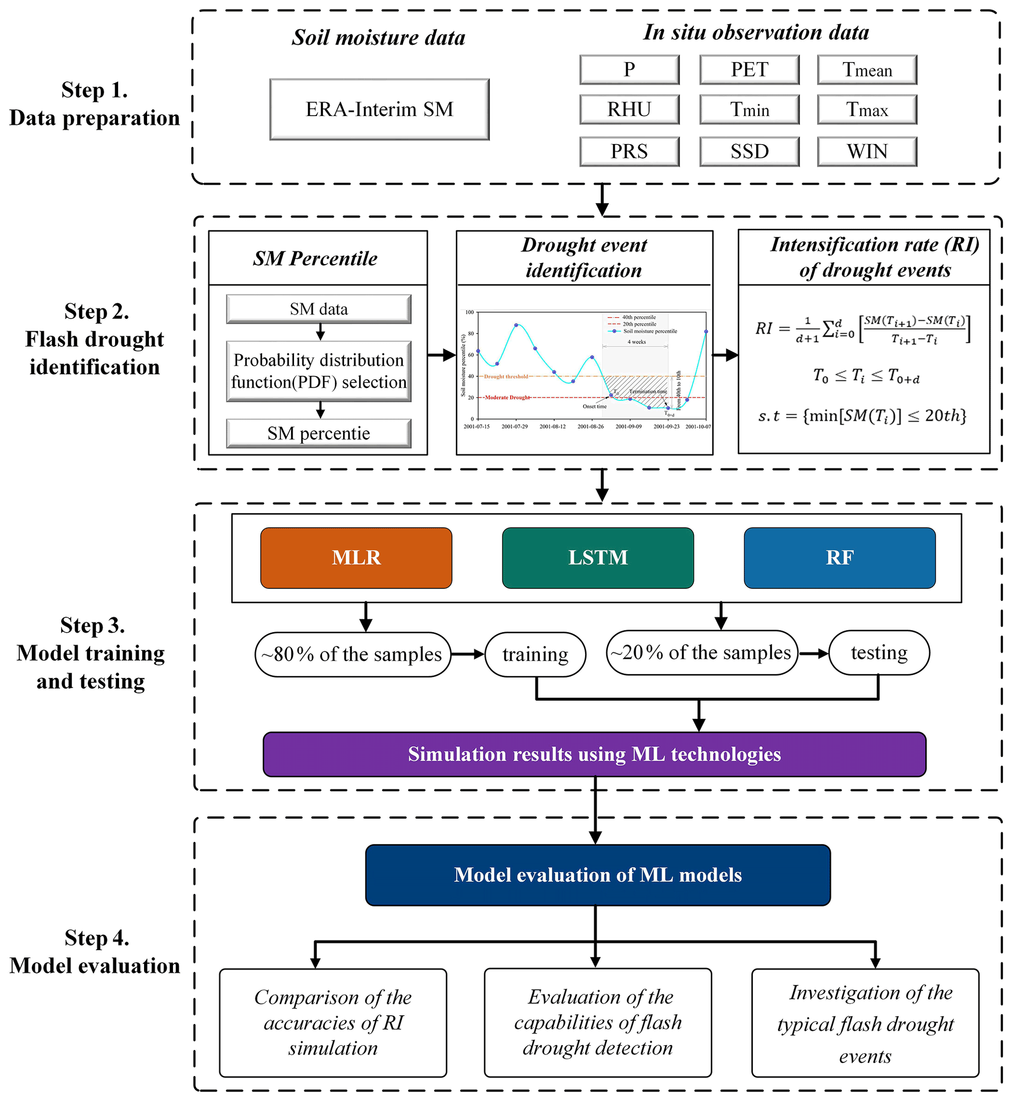
Figure 2The flow chart of evaluating the performances of ML models for flash drought detection.
4.1 Evaluation of the intensification rete of soil moisture
The capabilities of ML technologies in simulating the RI of soil moisture were assessed through intercomparison with the observed RI derived from ERA soil moisture. As shown in Fig. 3, higher RIs (up to the 12.5 percentile per week for certain areas) were mostly concentrated in the southern part of China, e.g., the east of QTP, the east of SW, and some regions of of MLYR. In contrast, lower RIs (less than the 5.0 percentile per week for some regions) were mainly distributed in the southern XJ and western NW areas. Given the spatial heterogeneity of soil moisture, Fig. 3b and c show the box plots of RI in different sub-regions, as well as the changes of empirical cumulative distribution function (ECDF) of RI. It can be seen that the lowest RIs were mostly located in the XJ region, with the median value of the 6.7 percentile per week. The highest RIs were distributed in the SW region, with the median value of the 12.5 percentile per week.
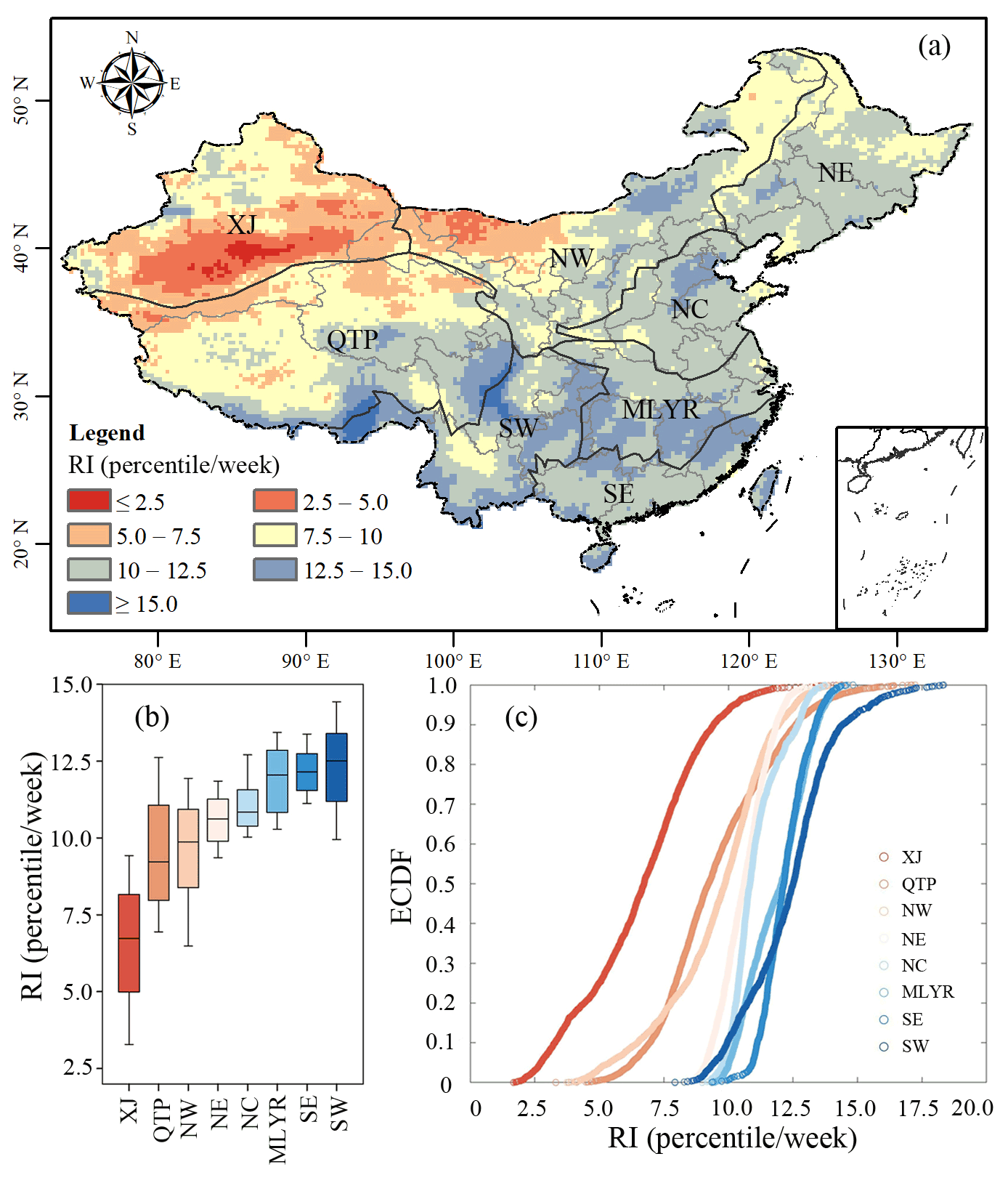
Figure 3(a) Spatial distribution of the average rate of intensification (RI) during 1979–2016. (b) Box plots of the average RI and (c) empirical cumulative probability distribution function (ECDF) of the average RI over different sub-regions in the study area. The sub-regions are Northeast China (NE), Northern China (NC), the middle and lower reaches of the Yangtze River region (MLYR), Southeastern China (SE), Northwestern China (NW), Southwestern China (SW), Qinghai–Tibet Plateau (QTP), and Xinjiang (XJ).
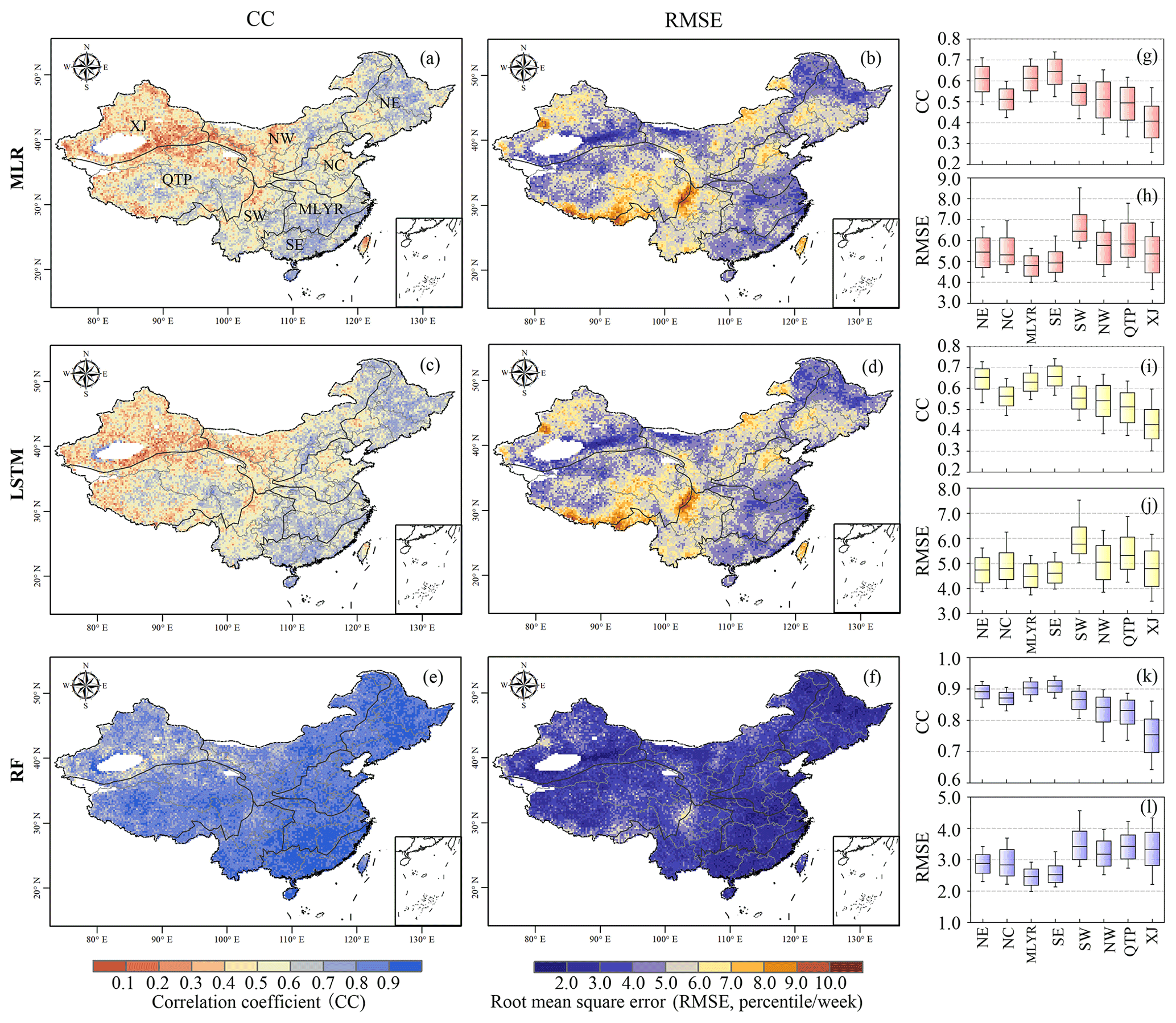
Figure 4Spatial distribution of correlation coefficient (CC) and root mean square error (RMSE) of the estimated RI by (a–b) MLR, (c–d) LSTM, and (e–f) RF models against the observed RI. (g–l) Box plots of the CC and RMSE for eight sub-regions, respectively.
Based on the observed RI and simulations from three ML technologies (i.e., MLR, LSTM, and RF), Fig. 4 shows the spatial distribution of CC and RMSE for the estimated RI against the observed RI in the testing phases during 1979–2016. For most parts of NE, SE, and MLYR regions, there was generally a good agreement between the MLR-simulated RI and observed RI with average CC values above 0.6 and average RMSE values below the 5.0 percentile per week (Fig. 4a and b). The weaker correlations were mainly distributed in the southern part of XJ, as well as northern and western QTP. A similar spatial pattern was also found for LSTM simulated RI but with overall boosted consistency (Fig. 4c and d). Among the three ML models, the RF performed best, as shown in Fig. 5e and f. Average CC values between RF-simulated RI and the observed RI in most areas of China were more than 0.8, and the average RMSEs were less than the 4.0 percentile per week. Especially, the excellent estimations were found in the SE region, with an average CC of 0.90 and average RMSE of the 2.6 percentile per week, while unsatisfying results were located in the XJ region, with an average CC of 0.75 and average RMSE of the 3.3 percentile per week.
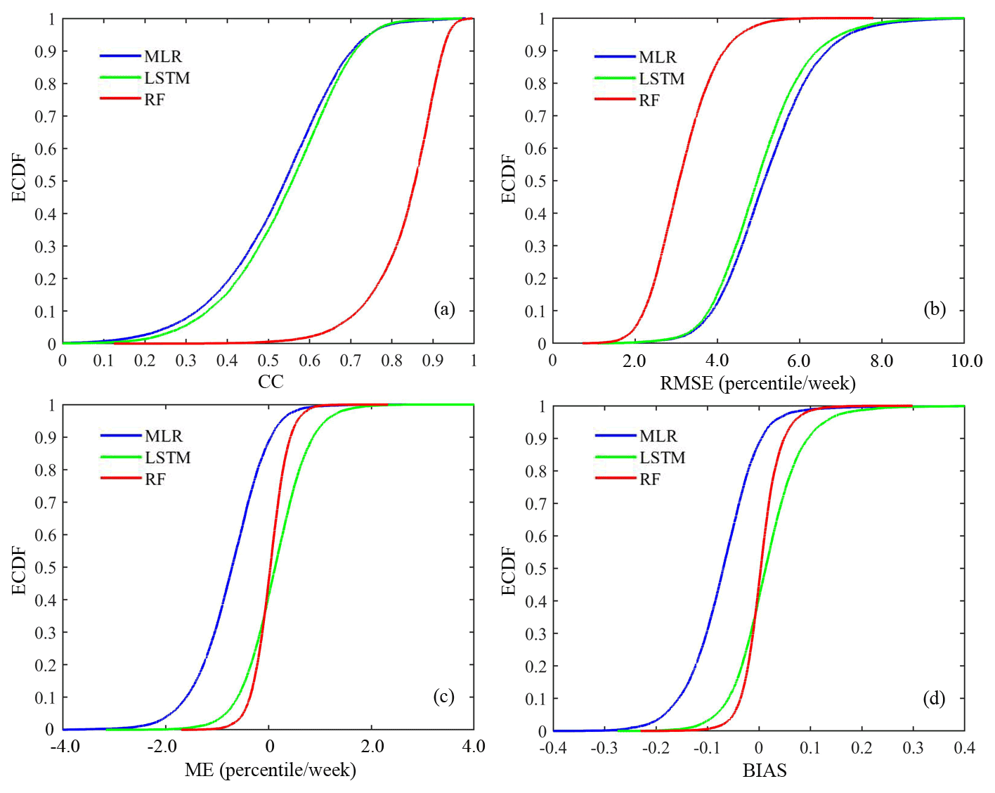
Figure 5Empirical cumulative distribution function (ECDF) of (a) correlation coefficient (CC), (b) root mean squared error (RMSE), (c) mean error (ME), and (d) relative bias (BIAS) of the RI estimated by the MLR, LSTM, and RF models against observed RI.
Figure 5 presents the ECDF of four evaluation coefficients (i.e., CC, RMSE, ME, and BIAS) of the estimated RI against the observed RI for all grids in China. It can be seen that the ECDF of CC and RMSE derived from the MLR and LSTM models were close to each other in different percentile intervals (Fig. 5a and b), and as for ME and BIAS, the LSTM presented better estimations given the lower values of ME and BIAS (Fig. 5c and d). As for the RF model, the CC values were much higher than those of MLR and LSTM models, combined with lower values in terms of RMSE, ME, and BIAS. The above analysis suggests that for RI estimation, the RF model was superior to MLR and LSTM models.
4.2 Comparison of the RI of flash droughts and slowly evolving droughts
RI is an important metric for distinguishing flash droughts from traditional slowly evolving droughts. To evaluate the capabilities of three ML in detecting drought events, we analyzed the correlation between model-simulated RI and observed RI for flash droughts and conventional droughts, respectively (Fig. 6). For flash droughts, the MLR and LSTM models displayed a similar spatial pattern, where higher CC values (up to 0.6 for some areas) were mainly located in the MLYR and SE regions, and correlations in the XJ and NW districts were generally weak (Fig. 6a and c). As for the RF model, except for some parts of the XJ region, it presented a rather high consistency with observed RI (CC values reach up to 0.9) in most areas of China. As for the case of traditional droughts, the MLR and LSTM methods showed a weak correlation over the whole of China (Fig. 6b and d). With respect to the RF model, the CC values overall increased in comparison with MLR and LSTM, with significant changes (the CC values increased by approximately 0.4) in SE and SW regions.

Figure 6Spatial distribution of correlation coefficient (CC) of the rate of intensification (RI) estimated by (a–b) MLR, (c–d) LSTM, and (e–f) RF models against the observed RI under flash droughts and slowly evolving droughts.
Figure 7 further exhibits the absolute errors and relative errors between the estimated RI and observed RI at four percentile intervals: 0th–5th, 5th–10th, 10th–15th, and 15th–20th percentile per week. According to the aforementioned flash drought identification method, droughts with an RI below the 5th percentile can be viewed as traditional droughts, while above the 10th percentile they can be classified as flash droughts. For flash droughts, the good (absolute error below the 1.0 percentile per week) performance of MLR was observed in NE, SE, SW, and MLYR regions, while unsatisfying results were found in XJ and NW areas (Fig. 7j–l). As for the slowly evolving droughts, the higher estimated accuracy (absolute error below the 1.0 percentile per week) was mainly concentrated in XJ and NW regions; however, the unsatisfying results (absolute error over the 10th percentile per week) were mostly located in the SW region (Fig. 7a–c). In addition, a satisfactory estimation of RI, with value ranges of the 5th–10th and 10th–15th percentile per week, was presented in most parts of China. Based on the above analysis, it can be concluded the MLR, LSTM, and RF algorithms can simulate RI derived by flash drought in the NE, SE, SW, and MLYR regions well, while these methods displayed a good estimation accuracy of RI indicated by traditional drought in XJ and NW regions.
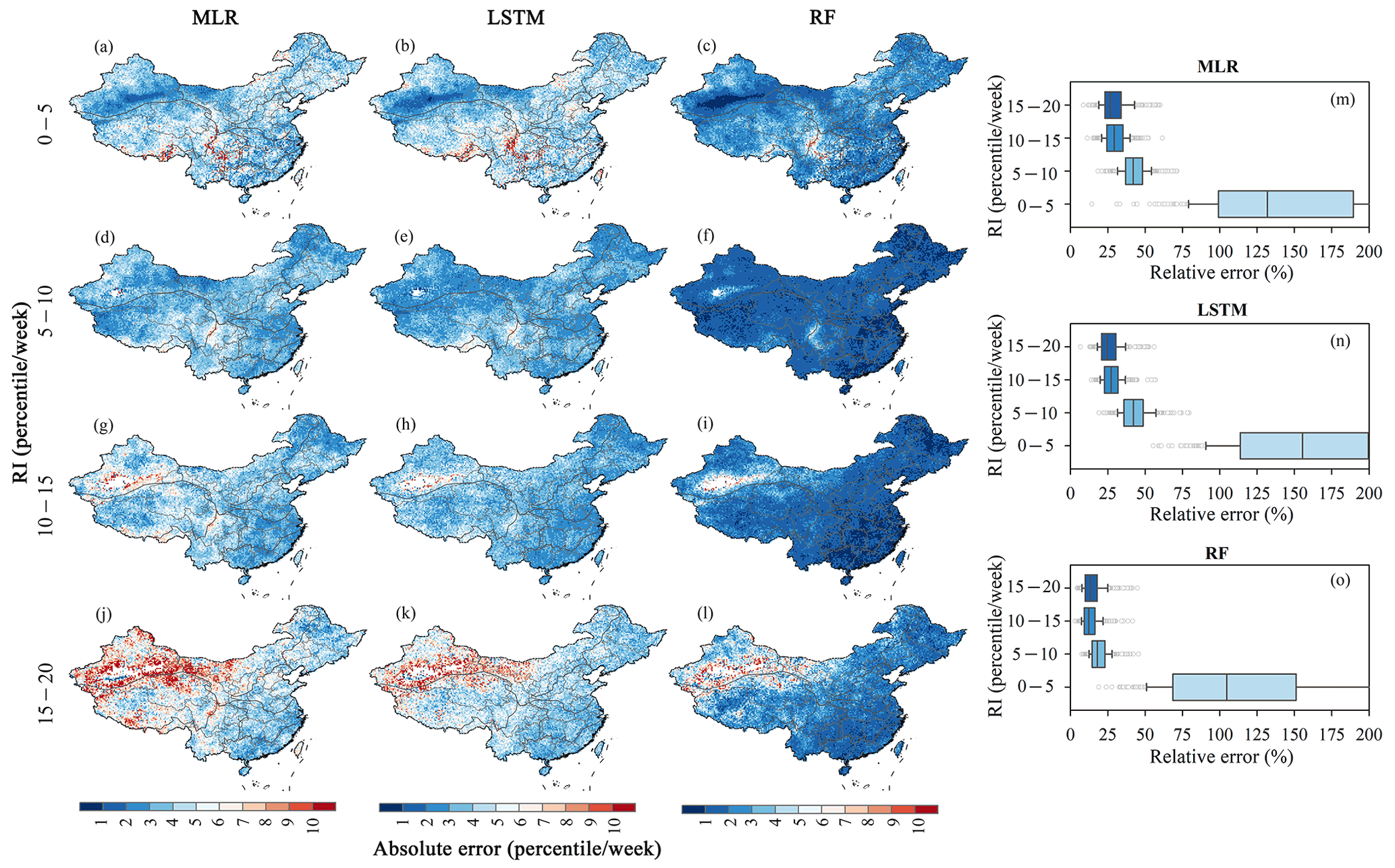
Figure 7Spatial pattern of the absolute errors and box plots of the relative errors of the RI estimated by the MLR, LSTM, and RF methods against observed RI at four percentile intervals.
Based on the above analysis, we further evaluated the capabilities of the MLR, LSTM, and RF models in capturing flash drought events and conventional drought events in eight different sub-regions using three skill scores (i.e., POD, FAR, and CSI) (Fig. 8). For flash droughts, the average POD (FAR) of the MLR and LSTM models ranged from 0.58 to 0.88 (0.08 to 0.41) and 0.68 to 0.94 (0.10 to 0.44), respectively, which were much lower (higher) than those of the RF algorithm (Fig. 8a and b). Likewise, the CSI of the MLR and LSTM models was much lower than that of the RF methods. Figure 8c and d present the cases of slowly evolving droughts. It can be seen that the POD (FAR) of the MLR (LSTM) model ranged from 0.41 to 0.70 (0.32 to 0.71) and 0.27 to 0.61 (0.30 to 0.66), respectively, while the values of the RF approach varied from 0.34 to 0.72 (0.11 to 0.19). In terms of the CSI, the MLR and LSTM presented unsatisfying performances compared to the RF model, with average values of 0.34, 0.30, and 0.51, respectively. Spatially, with the highest POD and CSI scores and the lowest FAR scores, the SE region exhibited the best detection results, and poor performances were in the XJ region. In general, all three ML models provided more reliable information in detecting flash droughts than traditional droughts. Meanwhile, the RF is more recommended for use, given its high skill scores and low false alarms in drought detection.
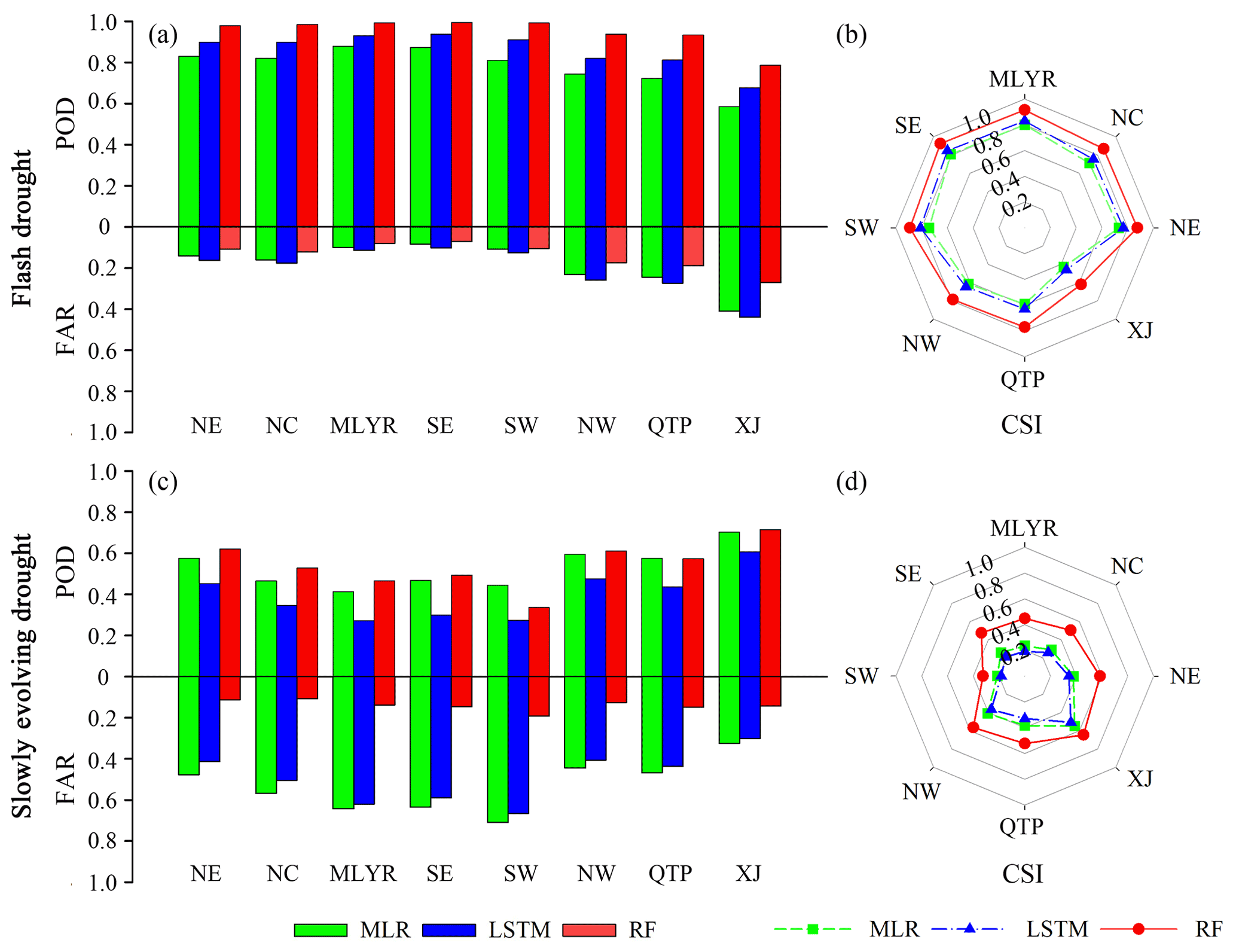
Figure 8Skill scores of POD, FAR, and CSI for flash droughts and slowly evolving droughts based on the MLR, LSTM, and RF models in eight sub-regions.
4.3 Spatiotemporal evolution of typical flash drought events
The ability of capturing the migration trajectories of droughts over time and space is also important when evaluating the capabilities of candidate ML models in drought detection. Figure 9a displays the time series of flash drought area and conventional drought area derived from ERA-Interim SM data during 1979–2016. As expected, the areas of slowly evolving droughts overwhelmingly exceeded those of flash droughts, and the areal gaps were further enlarged after 2003. Figure 9b and c exhibit the weekly variation of drought area in 2006 (the largest flash drought during the past 38 years with 11.73 % of the area affected) and 2013. The results show that summer and autumn were two major seasons for which the area of flash droughts and traditional drought developed towards different directions (increase or decrease). Given this, a specific investigation on the behaviors of MLR, LSTM, and RF in the summer and autumn of 2006 and 2013 was conducted to explore the capacities of the three ML models in monitoring the spatiotemporal migration trajectories of flash droughts. Figure 10 shows the spatial distribution of the soil moisture percentile (first column), observed RI (second column), and simulated RI by ML models (third to fifth column). From the perspective of the observed RI, the summer flash droughts mainly hit the NW, NC, SW, and MLYR regions of China on 17 June 2006 (Fig. 10b). Then the signal of flash droughts migrated towards the NE and SE regions on 23 September (Fig. 10g and l). Similarly, the 2013 summer flash droughts were mostly concentrated in MLYR areas, with an average RI of the 15.2 percentile per week (Fig. 10q). After 12 weeks, the flash droughts occurred on 17 October and were mainly located in the SW area (Fig. 10v and aa). In terms of the accuracy of RI simulation, the MLR-estimated RI was generally higher than the observed RI in the SE and SW regions (Fig. 10h, m, w, and ab). Compared to the MLR algorithm, the simulated RI by the LSTM and RF approaches basically followed a pattern nearly consistent with the observed RI, suggesting that they were superior to MLR in monitoring flash droughts.

Figure 9Time series of flash drought area and slowly evolving drought area derived from ERA SM series during 1979–2016, as well as in the typical years of 2006 and 2013.
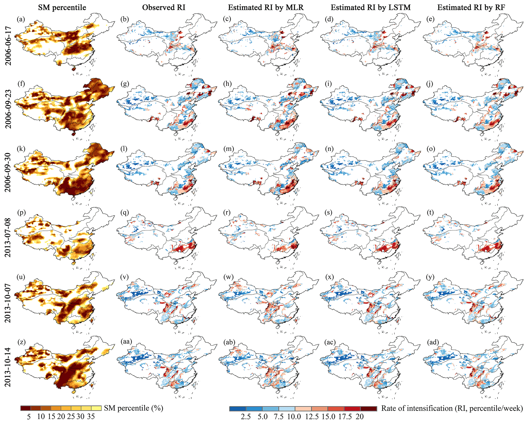
Figure 10Spatial evolution of the weekly soil moisture percentile, the observed RI, and estimated RI from MLR, LSTM, and RF models over the study area in summer and autumn of 2006 and 2013.
5.1 Performance of ML technologies for RI estimation
We evaluated three ML technologies in this study and found RF provided the best estimations of RI, with higher CC and lower RMSE compared to the observed RI (Figs. 4 and 5). It is not surprising that MLR did not perform well given its simple linear regression scheme, which is insufficient to describe the complicated nonlinear relationships of variables. With complicated model structures, the LSTM performed slightly better than MLR, but its efficiency is not optimistic either given the time-consuming calculations of the model. One possible reason lies in the fact that the model requires the input and output data to have the same time step. In this study, the output of RI reflected the average depletion rate of soil moisture during the onset–development stage, leading to inconsistent temporal steps between output and input (i.e., meteorological variables), as mentioned in runoff prediction modeling (Xiang et al., 2020). Several previous studies also found the good behaviors of RF in constructing the nonlinear interactions between soil moisture and different land surface variables and its strong capabilities for capturing the spatiotemporal variability of soil moisture (Zhao et al., 2017). For example, Fathololoumi et al. (2020) found due to the strong capability of considering the complex linear and nonlinear relationships between soil moisture and land surface properties, RF outperforms MLR, triangle regression, inverse distance weighting, and ordinary kriging techniques in estimating the variation of soil moisture in a semi-arid mountainous region. Rahmati et al. (2020) found the RF had excellent performances in mapping the agricultural drought hazards compared to other machine learning technologies, including the classification and regression trees, boosted regression trees, multivariate adaptive regression splines, flexible discriminant analysis, and support vector machines. The outstanding performance of RF could be attributed to the mathematical algorithm of the model, which enables high classification accuracy, unbiased determination of generation error with the out-of-bag method, and high efficiency in extracting important information from complicated nonlinear interactions of variables in handling high-dimensional datasets (Naghibi et al., 2016; Rodriguez-Galiano et al., 2012; Wang et al., 2015).
Regarding the spatial heterogeneity of RI, we found the RF performed best in southern China, while the estimation errors were high in the XJ region. This might be related to the local climate and soil conditions. Figure 11 compares the variation of soil moisture and moisture-related (i.e., P and RHU) and energy-related (i.e., PET, Tmean, Tmax, Tmin, PRS, SSD, and WIN) meteorological factors in adjacent weeks (i.e., T0−7–T0+7) to the onset of drought events during 1979–2016 in XJ and SW regions of China. The XJ region is climatically drier with relatively thick soil layers and sparse vegetation, and this climate and underlying surface conditions may not be beneficial to induce a rapid response of soil moisture to meteorological anomalies. From Fig. 11a, c, and e, we can see that for the XJ region, the variation of soil moisture was not consistent with the changes of meteorological anomalies for flash droughts. The sharp decline of soil moisture (with the value changing from the 55.05 to 8.87 percentile within 2 weeks) in Fig. 11a is a typically rapid rate of intensification for flash droughts. However, the meteorological variables did not change synchronously and even presented lagging variations (e.g., P, PET, and Tmean) after the onset of flash drought. By contrast, the consistency between soil moisture and meteorological variables was considerably improved for slowly evolving droughts (Fig. 11b, d, and f). As expected, the consistency degree was generally high in the SW region, with better behaviors for flash droughts. As shown in Fig. 11g, soil moisture decreased from the 55.25 to 10.54 percentile within 2 weeks. Regarding meteorological variables, both P and RHU showed relatively stable negative anomalies (e.g., the value of P anomaly and RHU anomaly at T0 was −0.43, and −0.69, respectively), and energy-related variables (e.g., PET, T, WIN) presented continuously positive anomalies (e.g., the value of Tmean anomaly and PET anomaly at T0 was 0.28 and 0.59, respectively). All of this contributes to the rapid decline of soil moisture. Different from the XJ region, the SW region belongs to a humid climate zone with abundant soil moisture from the top to deep layers, accompanied with dense vegetation and well-developed root systems. In the joint effects of P deficit and high temperatures or heat wave (Fig. 11g, i, and k), the capacity of evapotranspiration from vegetation could be enhanced in a very short time period, leading to a rapid response of soil moisture to the unusual climate conditions.
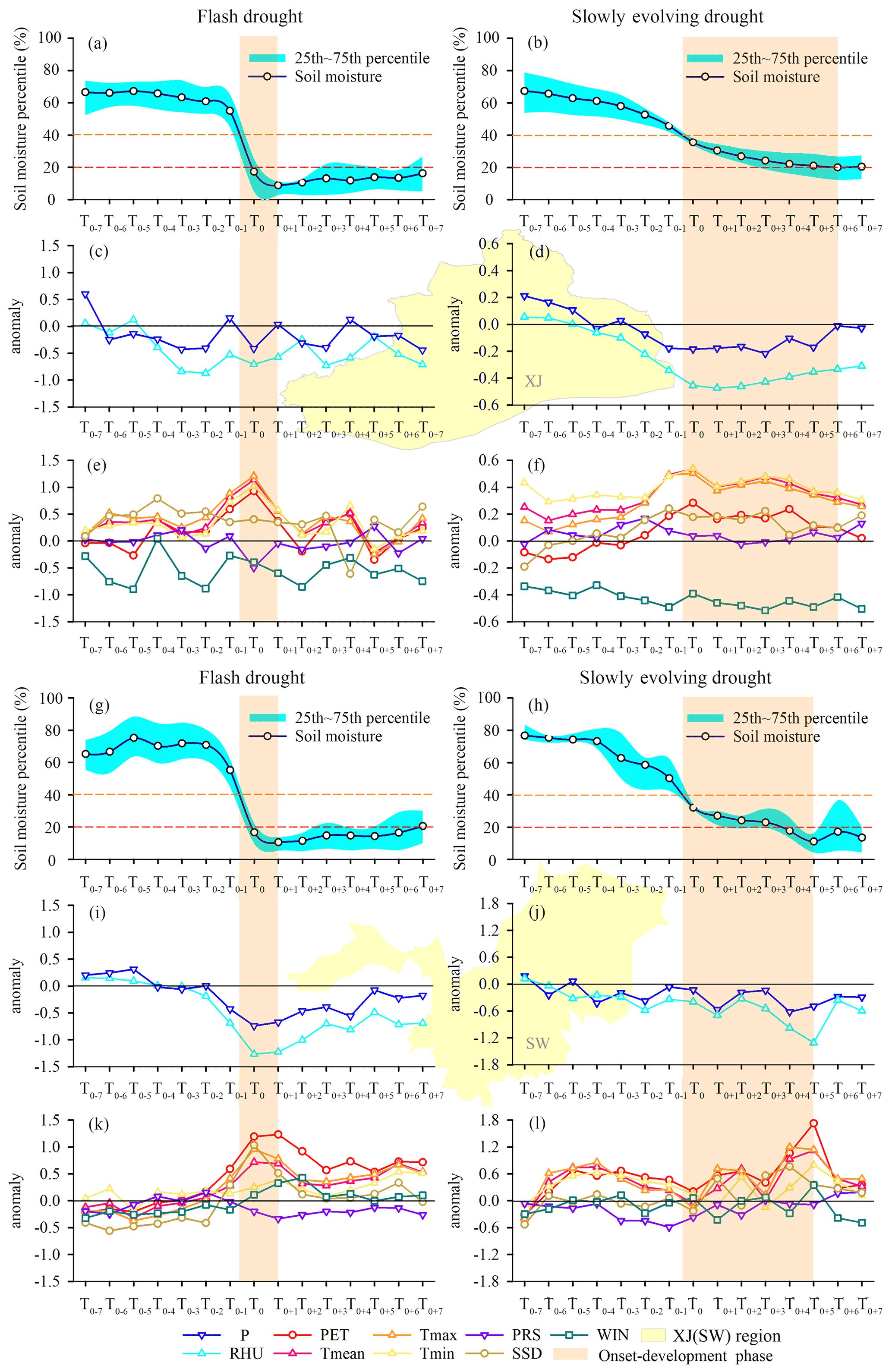
Figure 11Time series of weekly soil moisture percentile and moisture-related (i.e., P and RHU) and energy-related (i.e., PET, Tmean, Tmax, Tmin, PRS, SSD, and WIN) climate factors in the adjacent week (T0−7–T0+7) to drought onset during 1979–2016 for flash droughts and slowly developing droughts in the XJ and SW regions. The blue shading (Fig. 11a, b, g, and h) denotes the 25th–75th percentile range of soil moisture values. The orange shading in all 12 panels represent the onset–development phase of drought.
5.2 Comparison of ML technologies for flash droughts and slowly evolving droughts
In this study, all three ML models produced better RI estimations of flash droughts than those of conventional droughts (Figs. 6 and 8), suggesting that they are more competent in monitoring the rapid onset of droughts. From the perspective of physical mechanisms, the formation of conventional droughts commonly take a rather long time (e.g., several months or years), and they are driven by a variety of meteorological factors (Mishra and Singh, 2010). For instance, precipitation deficits, enhanced evaporative demand (high temperature or heat wave), and their joint or alternant effects all possibly contribute to a cumulative effect on soil moisture and lead to agricultural drought (Otkin et al., 2018; Yuan et al., 2017). Given the different climate and underlying conditions, the response time of the hydrological system can be different, manifested as varied timescales of droughts (Zhu et al., 2021). Particularly, the driving forces of slowly evolving droughts could be more diverse when considering the abnormal atmospheric circulation, which is the origin of meteorological droughts and is also responsible for soil moisture drought. The large-scale circulation can modify precipitation's frequency and intensity and increase wind speed, temperature, and evaporative demand (Hoerling et al., 2014; Mo and Lettenmaier, 2015). Several studies showed that the occurrence of droughts is related to large-scale circulation factors. Wang et al. (2016) found that under the background of El Niño of 2015/2016, a positive summer Eurasian teleconnection pattern is beneficial to anomalous northerly currents and weakening of the East Asia summer monsoon, which leads to extreme droughts over northern China. The 2017 drought in north-eastern China was caused by a strong positive phase of the Arctic Oscillation (AO) in March (Zeng et al., 2019). Also, 2000–2012 interdecadal drought in eastern Africa is closely linked to the anomalies of surface sea temperature (SST) in the tropical Pacific basin (Lyon and De Witt, 2012). These studies indicate that droughts essentially are resulted from sea–atmosphere and land–atmosphere interactions. In general, the complicated driving forces of slowly evolving droughts at varying timescales make it difficult to simulate the variation of soil moisture from a climatic perspective.
In a different manner, flash drought particularly refers to the time period in which rapid depletion of soil moisture occurs, which usually requires simultaneous anomalies in precipitation, relative humidity, potential evapotranspiration, temperature, sunshine duration, wind speed, and other meteorological variables to integrate into strong climatic forces (Liu et al., 2020a; Hobbins et al., 2016; Hunt et al., 2014). This rigorous atmospheric driving condition theoretically would not sustain for a long time, and a pentad or weekly timescale is recommended for monitoring flash droughts. Meanwhile, they have a stronger meteorological forcing than conventional droughts (Ford and Labosier, 2017), indicating a close interaction between RI of flash drought and these local meteorological conditions. This may be one possible reason for the higher accuracies of RI prediction for flash droughts. Comparison of the individual roles of precipitation (representing the water supply condition) and PET (representing the limits of evaporative demand) in formulating flash droughts and traditional droughts also showed this difference. Taking the case of the MLR method as an example, Fig. 12 exhibits the weights of P and PET anomalies in the adjacent weeks (as T0−7–T0+7 in Fig. 11) to drought onset for the XJ and SW regions. As shown, the weights of P and PET anomalies for flash droughts were generally higher than those of traditional droughts, suggesting a closer relationship between meteorological variables (i.e., P and PET) and flash droughts. Meanwhile, regional differences associated with the individual roles of P and PET were also observed. For the XJ region, the weights of negative P anomaly were generally high at the beginning of two types of drought, while the maximum weight of the positive PET anomaly occurred almost after drought onset. As for the SW region, both the negative P anomalies and the positive PET anomalies presented high weights during the onset time of droughts. The results suggested that P deficit played an important role during drought onset in the XJ region, and for the SW region, the lack of precipitation and elevated evaporative demand both played important roles for the occurrence of droughts, and this synchronously combined effect on the depletion of soil moisture is particularly significant for flash droughts. In general, the ML models are more competent in capturing the variation of RI for flash droughts than the slowly evolving drought due to the close causative relationship between meteorological forces and the former drought type.
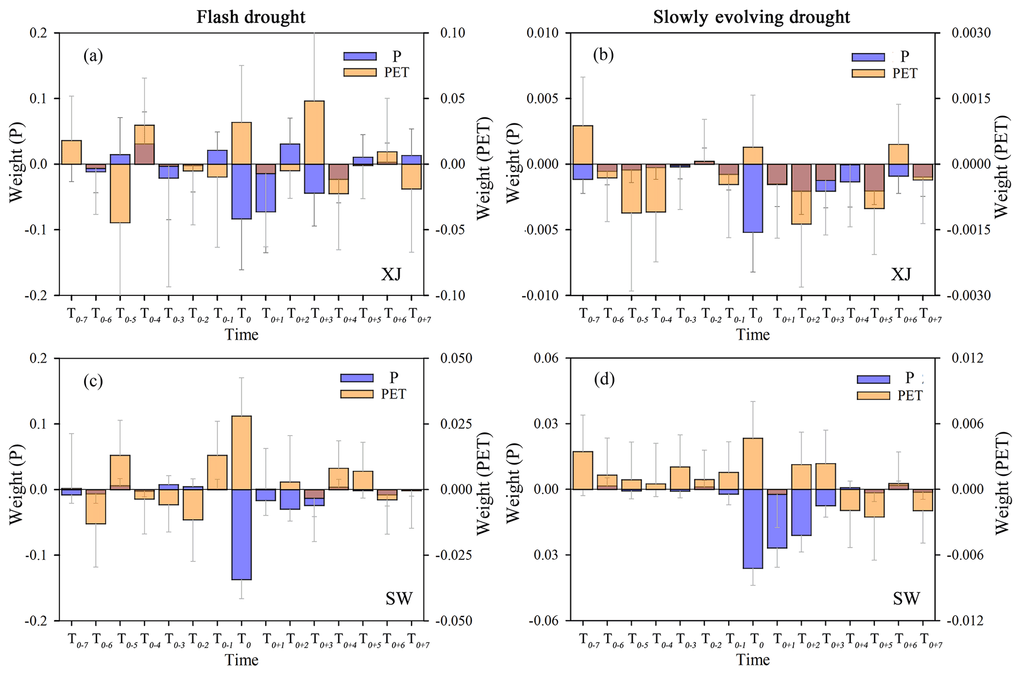
Figure 12The weights of P (blue bar) and PET (yellow bar) for flash droughts and slowly evolving droughts based on the MLR method in adjacent weeks to drought onset in the XJ and SW regions. T0−1 denotes 1 week prior to the onset time, while T0+1 represent 1 week after the onset time.
5.3 Influence of definitions on RI simulation results
As we mentioned before, two main definitions of flash drought were proposed by Mo et al. (2015, 2016) and Otkin et al. (2018). The two definitions were compared in several former studies in their effects on identifying flash droughts. Wang and Yuan (2018) investigated PDFD and HWFD over China during the growing seasons in 1979–2010 and found that PDFD tends to occur in southern China, where moisture supply is sufficient, while HWFD is more likely to occur in semi-arid regions (e.g., northern China). Liu et al. (2020a) showed the strengths and limitations of the soil moisture rapid-intensification approach and the multiple variable threshold methods (i.e., identification methods for PDFD and HWFD events). For flash drought based on the rate of intensification approach (RIFD), the average frequency of occurrence (FOC) varied between 3 % and 10 %, while the average FOC of HWFD and PDFD was less than 3 % and ranged from 4 % to 6 %, respectively, suggesting different types of identification would affect results of FOC to some extent. Even though the choice of definition may lead to different results of flash drought frequency, the difference would not be significant, no matter which kinds of definitions are applied. Osman et al. (2021) compared several definitions (e.g., soil moisture percentile drop (SMPD), standardized evaporative stress ratio (SEER), heat-wave-driven (HWD), and precipitation-deficit-driven (PDD)) to investigate the sensitivity of identification results to the choice of definition, and research showed that the spatial distribution of some typical flash drought events is well captured by most of the evaluated definitions. In short, diverse definitions of flash drought would not affect the feasibility of analyzing the flash drought simulation from the perspective of meteorological forcing. In this study, we focused on evaluating the performance of three ML algorithms on RI simulation and their ability in identifying flash droughts. Indeed, the ML models have a weak advantage in discovering the physical mechanism of flash droughts. However, the interaction between flash drought and the corresponding meteorological anomaly was first analyzed, which provided a reference to develop a physical-based model to simulate flash drought in the future.
5.4 Impact of flash droughts on agricultural production
Flash drought is a rapid onset and high-intensity extreme drought. Its onset and development are generally not only due to the precipitation deficit, but also owing to other meteorological anomalies (e.g., high temperature, strong wind, and abundant sunshine) that enhanced evaporative demand (Otkin et al., 2013; Anderson et al. 2013). These moisture-limited and energy-limited factors work together to quickly decrease soil moisture, gradually increase vegetation stress, and then induce the onset of flash drought (Hunt et al., 2009; Ford et al., 2015). This situation is most likely to occur during the growing season of vegetation and crops with the highest evaporative demand. When flash drought occurs during the critical stage of crop development (e.g., pollination in corn and the grain filling stage in soybeans), it may lead to a large agricultural reduction (Otkin et al., 2013; Hunt et al., 2014). For instance, the 2012 flash drought in the Midwest United States was an expensive natural disaster with agricultural losses of about USD 7.62 billion (Hoerling et al., 2014). All in all, the occurrence of flash drought poses a potential threat to agricultural production. It is worth mentioning the effects of flash drought on crop yield are different from those of conventional drought. With the rapid onset of flash drought, farmers and ranchers have limited time to prepare for its detrimental effects; thus, it may result in a large reduction in crop yield (Otkin et al., 2016), whereas long-last traditional drought has persistent adverse impacts on agricultural production. Generally, the impact of flash drought on agricultural production is more severe than slowly developing droughts during a short period. However, it is necessary to conduct comprehensive evaluations of their effects combined with the actual drought status and background field. In addition, the accurate prediction of the RI of these droughts will contribute to mitigating the negative impact of flash droughts on agriculture.
Based on the depletion rate of soil moisture derived from the ERA-Interim dataset, we identified flash droughts across China during 1979–2016. Furthermore, the linear and nonlinear relationships between ERA-Interim soil moisture and multiple climate variables were constructed using the MLR, LSTM, and RF technologies. On this basis, we evaluated the performance of these models in estimating the rate of intensification (RI) of soil moisture and analyzed their capabilities in flash drought detection. Overall, the RF model displayed the best performance for the whole of China, which was much better than that of MLR and LSTM models. The highest results estimated by RF were in the NE region, with an average CC of 0.90 and average RMSE of the 2.6 percentile per week, while the lowest estimations were found in the XJ area, with an average CC of 0.75 and average RMSE of the 3.3 percentile per week. A specific investigation on the summer and autumn droughts in 2006 and 2013 indicated that RF and LSTM can well reveal the spatial patterns of RI. They were able to provide a better simulation of flash drought relative to MLR with the lowest estimations. Furthermore, these ML methods displayed a relatively higher detection capacity of flash droughts than that of traditional slowly evolving droughts. The RF model was recommended to simulate flash drought by considering the multiple meteorological variable anomalies in the adjacent time to drought onset. The POD, FAR, and CSI of flash drought captured by the RF were 0.93, 0.15, and 0.80, respectively. In terms of the meteorological driving mechanism of flash droughts, the negative precipitation (P) anomalies and positive potential evapotranspiration (PET) anomalies exhibited a stronger synergistic effect on flash droughts compared to slowly developing droughts. Such compound effects on flash drought also presented asymmetrical characteristics over two regions in China. For the XJ region, P deficit played a dominant role in driving the onset of droughts, while for the SW region, the lack of precipitation and elevated evaporative demand contributed almost equally to the occurrence of droughts. This work could help enhance the understanding of flash droughts and provide a reference for the application of ML models in simulating flash droughts.
ERA-Interim SM data used in this study are available through https://apps.ecmwf.int/datasets/data/interim-full-daily/levtype=sfc/ (ECMWF, 2022a). ERA-Interim SM data are gradually being superseded by the ERA5 reanalysis (https://cds.climate.copernicus.eu/cdsapp#!/dataset/reanalysis-era5-land, ECMWF, 2022b). Meteorological observation records can be downloaded from the China Meteorological Administration website (http://data.cma.cn/, CMA, 2021).
LinqZ carried out the analyses, wrote the manuscript, and prepared the figures. YL and LR designed the paper and supervised the formulation of this manuscript. AJT and YZ provided critical feedback and edits. LinyW and LZ prepared the data. SJ, XY, XF, and HY provided important suggestions. All authors discussed the results and contributed to the final paper.
At least one of the (co-)authors is a member of the editorial board of Hydrology and Earth System Sciences. The peer-review process was guided by an independent editor, and the authors also have no other competing interests to declare.
Publisher's note: Copernicus Publications remains neutral with regard to jurisdictional claims in published maps and institutional affiliations.
This research has been supported by the National Natural Science Foundation of China (grant no. U2243203), the Fundamental Research Funds for the Central Universities (grant nos. B200204029, B200203054, and 2019B05214), the National Natural Science Foundation of China (grant nos. 42171021, 41901037, and 42071040), the Postgraduate Research & Practice Innovation Program of Jiangsu Province (grant no. KYCX20_0468), and the Central Guidance for Local Science and Technology Development fund projects (grant no. 2021ZY0027).
This paper was edited by Rohini Kumar and reviewed by three anonymous referees.
Allen, C. D., Macalady, A. K., Chenchouni, H., Bachelet, D., Mcdowell, N., Vennetier, M., Kitzberger, T., Rigling, A., Breshears, D. D., and Hogg, E. H.: A global overview of drought and heat-induced tree mortality reveals emerging climate change risks for forests, Forest Ecol. Manag., 259, 660–684, https://doi.org/10.1016/j.foreco.2009.09.001, 2010.
Almendra-Martín, L., Martínez-Fernández, J., Piles, M., and González-Zamora, Á.: Comparison of gap-filling techniques applied to the CCI soil moisture database in Southern Europe, Remote Sens. Environ., 258, 112377, https://doi.org/10.1016/j.rse.2021.112377, 2021.
Aghakouchak, A., Farahmand, A., Melton, F. S., Teixeira, J., Anderson, M. C., Wardlow, B. D., and Hain, C. R.: Remote sensing of drought: Progress, challenges and opportunities, Rev. Geophys., 53, 452–480, https://doi.org/10.1002/2014RG000456, 2015.
Anderson, M. C., Hain, C., Otkin, J., Zhan, X., Mo, K., Svoboda, M., Wardlow, B., and Pimstein, A.: An intercomparison of drought indicators based on thermal remote sensing and NLDAS-2 simulations with US Drought Monitor classifications, J. Hydrometeorol., 14, 1035–1056, https://doi.org/10.1175/JHM-D-12-0140.1, 2013.
Bennett, A. and Nijssen, B.: Deep learned process parameterizations provide better representations of turbulent heat fluxes in hydrologic models, Water Resour. Res., 57, e2020WR029328, https://doi.org/10.1029/2020WR029328, 2021.
Breiman, L.: Random forests, Mach. Learn., 45, 5–32, https://doi.org/10.1023/A:1010933404324, 2001.
Chen, L., Gottschalck, J., Hartman, A., Miskus, D., Tinker, R., and Artusa, A.: Flash drought characteristics based on U.S. drought monitor, Atmosphere-Basel, 10, 498, https://doi.org/10.3390/atmos10090498, 2019.
Chen, S., Hong, Y., Cao, Q., Gourley, J. J., Kirstetter, P. E., and Yong, B.: Similarity and difference of the two successive v6 and v7 trmm multisatellite precipitation analysis performance over China, J. Geophys. Res.-Atmos., 118, 13060–13074, https://doi.org/10.1002/2013JD019964, 2013.
China Meteorological Administration (CMA): China land-surface meteorological daily dataset, CMA [data set], http://data.cma.cn/, last access: 20 October 2021.
Christian, J. I., Basara, J. B., Otkin, J. A., Hunt, E. D., Wakefeld, R. A., Flanagan, P. X., and Xiao, X.: A Methodology for Flash Drought Identification: Application of Flash Drought Frequency across the United States, J. Hydrometeorol., 20, 833–846, https://doi.org/10.1175/JHM-D-18-0198.1, 2019.
Cui, Y., Long, D., Hong, Y., Zeng, C., Zhou, J., Han, Z., Liu, R., and Wan, W.: Validation and reconstruction of FY-3B/MWRI soil moisture using an artificial neural network based on reconstructed MODIS optical products over the Tibetan Plateau, J. Hydrol. 543, 242–254, https://doi.org/10.1016/j.jhydrol.2016.10.005, 2016.
European Center for Medium-Range Weather Forecast (ECMWF): ERA Interim, Daily, ECMWF [data set], https://apps.ecmwf.int/datasets/data/interim-full-daily/levtype=sfc/, last access: 30 May 2022a.
European Center for Medium-Range Weather Forecast (ECMWF): ERA5-Land hourly data from 1950 to present, ECMWF [data set] https://cds.climate.copernicus.eu/cdsapp#!/dataset/reanalysis-era5-land, last acces: 10 June 2022b.
Fathololoumi, S., Vaezi, A. R., Alavipanah, S. K., Ghorbani, A., and Biswas, A.: Comparison of spectral and spatial-based approaches for mapping the local variation of soil moisture in a semi-arid mountainous area, Sci. Total Environ., 724, 138319, https://doi.org/10.1016/j.scitotenv.2020.138319, 2020.
Feng, Z., Niu, W., Tang, Z., Xu, Y., and Zhang, H.: Evolutionary artifical intelligence model via cooperation search algorithm and extreme learning machine for multiple scales nonstationary hydrological time series prediction, J. Hydrol., 595, 126062, https://doi.org/10.1016/j.jhydrol.2021.126062, 2021.
Ford, T. W. and Labosier, C. F.: Meteorological conditions associated with the onset of flash drought in the Eastern United States, Agr. Forest Meteorol., 247, 414–423, https://doi.org/10.1016/j.agrformet.2017.08.031, 2017.
Ford, T. W., McRoberts, D. B., Quiring, S. M., and Hall, R. E.: On the utility of in situ soil moisture observations for flash drought early warning in Oklahoma, USA, Geophys. Res. Lett., 42, 9790–9798, https://doi.org/10.1002/2015GL066600, 2015.
Feng, L., Li, T., and Yu, W.: Cause of severe droughts in southwest China during 1951–2010, Clim. Dynam., 43, 2033–2042, https://doi.org/10.1007/s00382-013-2026-z, 2014.
Hastie, T., Tibshirani, R., and Friedman, J.: The Elements of Statistical Learning: Date Mining, Inference, and Prediction, Springer Science & Bussiness Media, New York, NY 10013, USA, https://doi.org/10.1007/b94608, 2008.
Hobbins, M. T., Wood, A., McEvoy, D., Huntington, J., Morton, C., Anderson, M. C., and Hain, C.: The evaporative demand drought index. Part I: Linking drought evolution to variations in evaporative demand, J. Hydrometeorol., 17, 1745–1761, https://doi.org/10.1175/JHM-D-15-0121.1, 2016.
Hochreiter, S. and Schmidhuber, J.: Long short-term memory, Neural Comput., 9, 1735–1780, 1997.
Hoerling, M., Eischeid, J., Kumar, A., Leung, R., Mariotti, A., Mo, K., Schubert, S., and Seager, R.: Causes and Predictability of the 2012 Great Plains Drought, B. Am. Meteorol. Soc., 95, 269–282, https://doi.org/10.1175/BAMS-D-13-00055.1, 2014.
Hutengs, C. and Vohland, M.: Downscaling land surface temperatures at regional scales with random forest regression, Remote Sens. Environ., 178, 127–141, https://doi.org/10.1016/j.rse.2016.03.006, 2016.
Hunt, E. D., Hubbard, K. G., Wilhite, D. A., Arkebauer, T. J., and Dutcher, A. L.: The development and evaluation of a soil moisture index, Int. J. Climatol., 29, 747–759, https://doi.org/10.1002/joc.1749, 2009.
Hunt, E. D., Svoboda, M., Wardlow, B., Hubbard, K., Hayes, M., and Arkebauer, T.: Monitoring the effects of rapid onset of drought on non-irrigated maize with agronomic data and climate-based drought indices, Agr. Forest Meteorol., 191, 1–11, https://doi.org/10.1016/j.agrformet.2014.02.001, 2014.
IPCC: Climate change 2013: The Physical Science Basis, Working Group I Contribution to the Fifth Assessment Report of the Inter-governmental Panel on Climate Change, Cambridge University Press, Cambridge, United Kingdom and New York, NY, USA, 1535, https://www.ipcc.ch/site/assets/uploads/2017/09/WG1AR5_Frontmatter_FINAL.pdf (last access: 12 June 2022), 2013.
Li, J., Wang, Z., Wu, X., Chen, J., Guo, S., and Zhang, Z.: A new framework for tracking flash drought events in space and time, Catena, 194, 104763, https://doi.org/10.1016/j.catena.2020.104763, 2020.
Ling, X., Huang, Y., Guo, W., Wang, Y., Chen, C., Qiu, B., Ge, J., Qin, K., Xue, Y., and Peng, J.: Comprehensive evaluation of satellite-based and reanalysis soil moisture products using in situ observations over China, Hydrol. Earth Syst. Sci., 25, 4209–4229, https://doi.org/10.5194/hess-25-4209-2021, 2021.
Liu, Y., Zhu, Y., Ren, L., Otkin, J., and Jiang S.: Two Different Methods for Flash Drought Identification: Comparison of Their Strengths and Limitations, J. Hydrometeorol., 21, 691–704, https://doi.org/10.1175/JHM-D-19-0088.1, 2020a.
Liu, Y., Zhu, Y., Zhang, L., Ren, L., Yuan, F., Yang, X., and Jiang, S.: Flash droughts characterization over China: From a perspective of the rapid intensification rate, Sci. Total Environ., 704, 135373, https://doi.org/10.1016/j.scitotenv.2019.135373, 2020b.
Long, D., Bai, L., Yan, L., Zhang, C., Shi, C., Yang, W., Lei, H., Quan, J., Meng, X., and Shi, C.: Generation of spatially complete and daily continuous surface soil moisture of high spatial resolution, Remote Sens. Environ., 233, 111364, https://doi.org/10.1016/j.rse.2019.111364, 2019.
Lyon, B. and De Witt, D. G.: A recent and abrupt decline in the East African long rains, Geophys. Res. Lett., 39, L02702, https://doi.org/10.1029/2011GL050337, 2012.
Mishra, A. K. and Singh, V. P.: A review of drought concepts, J. Hydrol., 391, 202–216, https://doi.org/10.1016/j.jhydrol.2010.07.012, 2010.
Mo, K. C. and Lettenmaier, D. P.: Heat wave flash droughts in decline, Geophys. Res. Lett., 42, 2823–2829, https://doi.org/10.1002/2015GL064018, 2015.
Mo, K. C. and Lettenmaier, D. P.: Precipitation deficit flash droughts over the United States, J. Hydrometeorol., 17, 1169–1184, https://doi.org/10.1175/JHM-D-15-0158.1, 2016.
Mokhtar, A., Jalali, M., He, H., AI-Ansari, N., Elbeltagi, A., Alsafadi, K., Abdo, H. G., Sammen, S. S., Gyasi-Agyei, Y., and Rodrigo-Comino, J.: Estimation of SPEI Meteorological Drought Using Machine Learning Algorithms, IEEE Access, 9, 65503–65523, https://doi.org/10.1109/ACCESS.2021.3074305, 2021.
Naghibi, S. A., Pourghasemi, H. R., and Dixon, B.: GIS-based groundwater potential mapping using boosted regression tree, classification and regression tree, and random forest machine learning models in Iran, Environ. Monit. Assess., 188, 44, https://doi.org/10.1007/s10661-015-5049-6, 2016.
Noguera, I., Domínguez-Castro, F., and Vicente-Serrano, S. M.: Characteristics and trends of flash droughts in Spain, 1961–2018, Ann. NY Acad. Sci., 1472, 155–172, https://doi.org/10.1111/nyas.14365, 2020.
Osman, M., Zaitchik, B. F., Badr, H. S., Christian, J. I., Tadesse, T., Otkin, J. A., and Anderson, M. C.: Flash drought onset over the contiguous United States: sensitivity of inventories and trends to quantitative definitions, Hydrol. Earth Syst. Sci., 25, 565–581, https://doi.org/10.5194/hess-25-565-2021, 2021.
Otkin, J. A., Anderson, M. C., Hain, C., and Svoboda, M.: Examining the Relationship between Drought Development and Rapid Changes in the Evaporative Stress Index, J. Hydrometeorol., 15, 938–956, https://doi.org/10.1175/JHM-D-13-0110.1, 2013.
Otkin, J. A., Anderson, M. C., Hain, C., Svoboda, M., Johnson, D., Mueller, R., Tadesse, T., Wardlow, B., and Brown, J.: Assessing the evolution of soil moisture and vegetation conditions during the 2012United States flash drought, Agr. Forest Meteorol., 218–219, 230–242, https://doi.org/10.1016/j.agrformet.2015.12.065, 2016.
Otkin, J. A., Svoboda, M., Hunt, E. D., Ford, T. W., Anderson, M. C., Hain, C., and Basara, J. B.: Flash Droughts: A review and assessment of the challenges imposed by rapid onset droughts in the United States, B. Am. Meteorol. Soc., 99, 911–919, https://doi.org/10.1175/BAMS-D-17-0149.1, 2018.
Pendergrass, A., Meehl , G., Pulwarty, R., Hobbins , M., Hoell, A., Aghakouchak, A., Bonfils, C. J. W., Gallant, A. J. E., Hoerling, M., and Hoffmann, D.: Flash droughts present a new challenge for subseasonal-to-seasonal prediction, Nat. Clim. Change, 10, 191–199, https://doi.org/10.1038/s41558-020-0709-0, 2020.
Penman, H. L.: Natural evaporation from open water, bare soil and grass, P. R. Soc. A, 193, 120–145, https://doi.org/10.1098/rspa.1948.0037, 1948.
Pradhan, P., Tingsanchali, T., and Shrestha, S.: Evaluation of soil and water assessment tool and artificial neural network models for hydrologic simulation in different climatic regions of Asia, Sci. Total Environ., 701, 134308, https://doi.org/10.1016/j.scitotenv.2019.134308, 2020.
Rahmati, O., Falah, F., Dayal, K. S., Deo, R. C., Mohammadi, F., Biggs, T., Moghaddam, D. D., Naghibi, S. A., and Bui, D. T.: Machine learning approaches for spatial modeling of agricultural droughts in the south-east region of Queensland Australia, Sci. Total Environ., 699, 134230–134230, https://doi.org/10.1016/j.scitotenv.2019.134230, 2020.
Rodriguez-Galiano, V. F., Ghimire, B., Rogan, J., Chica-Olmo, M., and Rigol-Sanchez, J. P.: An assessment of the effectiveness of a random forest classifier for land-cover classification, ISPRS J. Photogramm. Remote Sens. 67, 93–104, https://doi.org/10.1016/j.isprsjprs.2011.11.002, 2012.
Sahoo, S., Russo, T. A., Elliott, J., and Foster, I.: Machine learning algorithms for modeling ground water level changes in agricultural regions of the U.S., Water Resour. Res., 53, 3878–3895, https://doi.org/10.1002/2016WR019933, 2017.
Schoppa, L., Disse, M., and Bachmair, S.: Evaluating the performance of random flood discharge simulation, J. Hydrol., 590, 125531, https://doi.org/10.1016/j.jhydrol.2020.125531, 2020.
Senay, G. B., Budde, M. B., Brown, J. F., and Verdin, J. P.: Mapping flash drought in the US: Southern Great Plains, In 22nd Conference on Hydrology, AMS, New Orleans, LA, 2008.
Svoboda, M., Lecomte, D., Hayes, M., Heim, R., Gleason, K., Angel, J., Rippey, B., Tinker, R., Palecki, M., Stooksbury, D., Miskus, D., and Stephens, S.: The Drought Monitor, B. Am. Meteorol. Soc., 83, 1181–1190, https://doi.org/10.1175/1520-0477-83.8.1181, 2002.
Sun, C. and Yang, S.: Persistent severe drought in southern China during winter–spring 2011: Large-scale circulation patterns and possible impacting factors, J. Geophys. Res., 117, D10112, https://doi.org/10.1029/2012JD017500, 2012.
Teuling, A. J.: A hot future for European droughts, Nat. Clim. Change, 8, 360–369, https://doi.org/10.1038/s41558-018-0154-5, 2018.
Trenberth, K. E., Dai, A., Schrier, G. V. D., Jones, P. D., Barichivich, J., Briffa K. R., and Sheffield, J.: Global warming and changes in drought, Nat. Clim. Change, 4, 17–22, https://doi.org/10.1038/nclimate2067, 2014.
Wang, A., Lettenmaier, D. P., and Sheffield, J.: Soil moisture drought in China, 1950–2006, J. Climate, 24, 3257–3271, https://doi.org/10.1175/2011JCLI3733.1, 2011.
Wang, H., Rogers, J. C., and Munroe, D. K.: Commonly used drought indices as indicators of soil moisture in China, J. Hydrometeorol., 16, 1397–1408, https://doi.org/10.1175/JHM-D-14-0076.1, 2015.
Wang, L. and Yuan, X.: Two types of flash drought and their connections with seasonal drought, Adv. Atmos.Sci., 35, 1478–1490, https://doi.org/10.1007/s00376-018-8047-0, 2018.
Wang, L., Yuan, X., Xie, Z., Wu, P., and Li, Y.: Increasing flash droughts over China during the recent global warming hiatus, Sci. Rep.-UK, 6, 30571, https://doi.org/10.1038/srep30571, 2016.
Xiang, Z., Yan, J., and Demir, I.: A rainfall-runoff model with LSTM-based sequence-to-sequence learning, Water Resour. Res., 56, e2019WR025326, https://doi.org/10.1029/2019WR025326, 2020.
Yang, S., Yang, D., Chen, J., Santisirisomboon, J., Lu, W., and Zhao, B.: A physical process and machine learning combined hydrological model for daily streamflow simulations of large watersheds with limited observation data, J. Hydrol., 590, 125206, https://doi.org/10.1016/j.jhydrol.2020.125206, 2020.
Yuan, X., Wang, L. Y., and Wood, E. F.: Anthropogenic intensification of southern African flash droughts as exemplified by the 2015/16 season, B. Am. Meteorol. Soc., 98, S86–S90, https://doi.org/10.1175/BAMS-D-17-0077.1, 2017.
Zeng, D. W., Yuan, X., and Roundy, J. K.: Effect of teleconnected land–atmosphere coupling on Northeast China persistent drought in spring–summer of 2017, J. Climate, 32, 7403–7420, https://doi.org/10.1175/JCLI-D-19-0175.1, 2019.
Zhang, L., Liu, Y., Ren, L., Teuling A. J., Zhang, X., Jiang, S., Yang, X., Wei, L., Zhong, F., and Zheng, L.: Reconstruction of ESA CCI satellite-derived soil moisture using an artificial neural network technology, Sci. Total Environ., 782, 146602, https://doi.org/10.1016/j.scitotenv.2021.146602, 2021.
Zhao, W., Li, A., Huang, P., Juelin, H., and Xianming, M.: Surface soil moisture relationship model construction based on random forest method, in: Proceedings of the 2017 IEEE International Geoscience and Remote Sensing Symposium (IGARSS), Fort Worth, TX, USA, 23–28 July 2017, 2019–2022, https://doi.org/10.1109/IGARSS.2017.8127378, 2017.
Zhu, Y., Liu, Y., Wang, W., Singh, V. P., and Ren, L.: A global perspective on the probability of propagation of drought: From meteorological to soil moisture, J. Hydrol., 603, 126907, https://doi.org/10.1016/j.jhydrol.2021.126907, 2021.