Modelling evaporation with local, regional and global BROOK90 frameworks: importance of parameterization and forcing

Evaporation plays an important role in the water balance on a different spatial scale. However, its direct and indirect measurements are globally scarce and accurate estimations are a challenging task. Thus the correct process approximation in modelling of the terrestrial evaporation plays a crucial part. A physically based 1D lumped soil–plant–atmosphere model (BROOK90) is applied to study the role of parameter selection and meteorological input for modelled evaporation on the point scale. Then, with the integration of the model into global, regional and local frameworks, we made cross-combinations out of their parameterization and forcing schemes to show and analyse their roles in the estimations of the evaporation.

Five sites with different land uses (grassland, cropland, deciduous broadleaf forest, two evergreen needleleaf forests) located in Saxony, Germany, were selected for the study. All tested combinations showed a good agreement with FLUXNET measurements (Kling–Gupta efficiency, KGE, values 0.35–0.80 for a daily scale). For most of the sites, the best results were found for the calibrated model with in situ meteorological input data, while the worst was observed for the global setup. The setups' performance in the vegetation period was much higher than for the winter period. Among the tested setups, the model parameterization showed higher spread in performance than meteorological forcings for fields and evergreen forests sites, while the opposite was noticed in deciduous forests. Analysis of the of evaporation components revealed that transpiration dominates (up to 65 %–75 %) in the vegetation period, while interception (in forests) and soil/snow evaporation (in fields) prevail in the winter months. Finally, it was found that different parameter sets impact model performance and redistribution of evaporation components throughout the whole year, while the influence of meteorological forcing was evident only in summer months.

1 Introduction

Evaporation as a water balance component plays an important role in the hydrological process at multiple spatial scales: from a single leaf to an entire catchment. As a result of mass and energy exchange between the soil–plant and atmosphere system, the global annual terrestrial evaporation amount yields approximately $\mathrm{2}/\mathrm{3}$ of the total precipitation (McDonald, 1961), showing however a large range even on a macroscale (Haddeland et al., 2011; Harding et al., 2011; Miralles et al., 2016). However, with the need of higher spatial and temporal resolution, the high variability of evaporation should be taken into account and properly addressed (Anderson et al., 2007; Baldocchi et al., 2001; Jung et al., 2011; Pan et al., 2020; Zhang et al., 2010). Thus, accurate estimates of evaporation on different scales, as well as advanced understanding of the process itself, are beneficial for planning, developing and monitoring of hydrologic agriculture and ecological systems, e.g. irrigation scheduling, water distribution systems, crop modelling, quantification of energy and moisture exchange between the land surface and the atmosphere (Fisher et al., 2017; McNally et al., 2019; Schulz et al., 2021). Apart from the total evaporation itself, it is sometimes necessary to assess and quantify its components (Chang et al., 2018; Lawrence et al., 2007; Leuning et al., 2008; Schulz et al., 2021), namely components, like transpiration, evaporation from the ground or snow surface, and evaporation of intercepted rain and snow from the canopy. However the partition of the evaporation is a subject of a large variability and depends not only on the location, but on scale as well (Wei et al., 2017; Zhang et al., 2017).

Various direct (i.e. porometer, eddy covariance and lysimeter) and indirect (catchment water balance, energy balance, theoretical models based on meteorological data) methods have been developed and used to measure evaporation at different spatio-temporal scales. Each method has its strengths and weaknesses, but what they have in common is that the results have limited representativeness. Namely, they are valid only within a certain space of scale and time (so-called “footprint”), which is usually quite small; thus only a local scale could be represented by it (Baldocchi, 1997; Wilson et al., 2001). Recently, these methods were extended to include remote-sensing techniques for the regional and global scale (Anderson et al., 2008; Leuning et al., 2008; Miralles et al., 2011, 2016), but the quality of the output products still possesses a potential for improvement (Pan et al., 2020; Zeng et al., 2012). Among the datasets of the in situ evaporation measurements, the FLUXNET network (http://www.fluxnet.ornl.gov, last access: 20 November 2021) provides eddy-covariance data from about 500 stations worldwide within FLUXNET2015 dataset (Pastorello et al., 2020) and still acts as the main driver in advancing evaporation research (Baldocchi et al., 2001; Jung et al., 2011; Mauder et al., 2018). Evaporation measurements are still scarcely available due to high costs and the problem of large-scale representability (e.g. in comparison to discharge measurements).

Hence, mathematical modelling in favour of its feasibility is a practical substitute. Besides empirical formulas (Cerro et al., 2021; Feng et al., 2016; Zeng et al., 2012), evaporation is often estimated by physically based models (Beven et al., 2021; Boulet et al., 2015; Liu et al., 2012; Mallick et al., 2018), in which Penman–Monteith (and Shuttleworth and Wallace extension) formula is one of the most frequently used. This approach reduces potential evaporation to an actual one accounting for the available water in the soil–plant system. Thus, it is incorporated into many land surface models and frameworks regardless of scale: local, regional or even global (Leuning et al., 2008; Mallick et al., 2018; Zink et al., 2017). Despite many efforts to improve evaporation models on different scales, large uncertainties still remain (Allen et al., 1998; Miralles et al., 2011; Mueller et al., 2011). In general, the sources of evaporation modelling (or more in general – hydrological modelling) uncertainties can be classified as follows: model structure and process representation, choice of an appropriate parameter set, meteorological input data, spatio-temporal mis-scaling and uncertainties of measurements for the model validation themselves (Mallick et al., 2018; Mauder et al., 2018; Mueller et al., 2011; Zhang et al., 2010). Studying these sources of uncertainties from different approaches and frameworks gained more attention in recent years; however most of these studies are limited by the focus on one single spatio-temporal scale (Chang et al., 2018; Jung et al., 2011; Liu et al., 2012). Only a few researchers focused on investigations of the uncertainties in multiple frameworks with multiple input datasets and simultaneously accounting for point, regional and global scales (Pan et al., 2020; Su et al., 2005; Winter and Eltahir, 2010).

Here we aim to extend the knowledge on soil–plant–atmosphere physically based lumped BROOK90 model, which we integrated into three frameworks. These frameworks use different “state-of-the-art” sources of data for the model parameterization and forcing which represent various spatial scales, namely global, regional and local. By mixing these different datasets and validating the simulated evaporation with eddy-covariance measurements, we show the impact of spatial scale of BROOK90 model parameterization and forcing on accuracy of evaporation simulations. Our main hypothesis is that the goodness of fit of the setups smoothly increases from global to local scale (for both parameterization and forcing). However, it was unclear how the scale combinations will perform, i.e. local meteorological data with global parameterization and vice versa. Therefore, this study presents the first qualitative analysis of the model input scale uncertainty in general, not going into deep quantitative analysis of single uncertainties using, for example, statistical bootstrapping or Monte Carlo simulations. It also possesses a practical outcome. Namely in a presence of limited resources and data, the global or regional BROOK90 frameworks deliver plausible evaporation estimations for a point (hydrological response unit) scale and where the user should put more attention – accurate parameterization or meteorological input. Thus, the outcome of this study provides a better understanding of the BROOK90 model as well as shows the directions to improve effectively evaporation simulations.

2 Material and methods

2.1 Study sites and eddy-covariance measurements

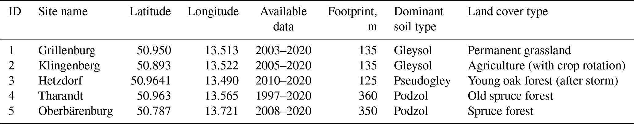
The evaluation of simulated evaporation was carried for five sites with various land covers and long-term eddy-covariance measurements (Fig. 1, Table 1). All selected towers are located in Saxony, Germany. The study area is characterized by temperate suboceanic/subcontinental climate (Cfb, Kottek et al., 2006). The average mean daily temperature varies between + 15 and + 20 ^∘C in summer months and between − 5 and + 5 ^∘C in winter months. The average annual precipitation varies between 750 and 960 mm. The measurements of atmospheric fluxes with standardized methods are operated by Technische Universität Dresden within ICOS and FLUXNET projects. In this study, we used daily evaporation values calculated from measured latent heat fluxes corrected for the observed site-specific energy budget closure gap. In general, from 10 (Hetzdorf) up to 23 (Tharandt) years of continuous time series are available.

The Grillenburg site (DE-Gri, the sensor height is 3 m above the ground) is a permanent and extensively managed (one to three cuts per year) flat-terrain grassland (mesophytic hay meadow). Regular mowing usually takes place in June and September. In the case of three cuts per year, the second one is usually done in July. Typical plant species include couch grass (Elymus repens), meadow foxtail (Alopecurus pratensis), common yarrow (Achillea millefolium), common sorrel (Rumex acetosa) and white clover (Trifolium repens). The area is generally used for forage and rarely for pasture. Vegetation height is measured once per week, with the lowest values (5–10 cm) measured at the beginning of growing season or after cutting and highest values (typically 30–40 cm, maximum 90 cm) in the summer before cutting. Although the leaf area index (LAI) was only occasionally measured, the significant correlation between vegetation height and LAI made it possible to interpolate the annual range. Therefore, the range of LAI was estimated between 0.25 and 5 m² m⁻² in the yearly course. The topography around the site promotes cold air deposition; thus daily minima of air temperature are often much lower than at the other sites. The site is mainly characterized by Gleysol soil that contains silty loam, loam and loamy silt as soil textures.

The Klingenberg site (DE-Kli, the sensor height is 3.5 m above the ground) is an intensively farmed arable land located 4 km south from the Tharandt forest (Fig. 1). This site is characterized by annual and inter-annual crop rotation of rapeseed (Brassica napus), winter wheat (Triticum aestivum), forage maize (Zea mays), spring barley (Hordeum vulgare) and winter barley (Hordeum vulgare) with occasional intercropping. As a result, plant cover, vegetation height, LAI and rooting depth varied greatly across time periods; i.e. measured annual maximum canopy height values vary between 0.7 and 2.2 m, and LAI could reach up to 6 m² m⁻². Soil properties and runoff behaviour are strongly influenced by tillage and fertilizer application. According to Ad-hoc-AG Boden (2005), the soil was classified as Gleysol and has a clay or loam texture.

The Hetzdorf site (DE-Hzd, the sensor height is 5 m (2010–2017), 11.5 m (2017–2021) and 17.5 m (since 2021) above the ground) is a young oak (Quercus robur) forest planted after the Kyrill storm in 2007, which caused severe windthrow (40 ha) in an old Norway spruce (Picea abies) forest. This site has a moderate slope to the north and a main wind direction to the south due to a gap in the surrounding old spruce forest. The young oak stand is approximately 8–10 m high (2021) and enclosed by spruce forest (up to 30 m height). Due to the high amount of deadwood and the young oak plantation until 2017, this ecosystem was a net CO₂ source, but since 2018 it has acted as a moderate CO₂ sink (Drought 2018 Team and ICOS Ecosystem Thematic Centre, 2020; Warm Winter 2020 Team and ICOS Ecosystem Thematic Centre, 2022). As a young growing site, LAI varies dynamically from year to year and was only measured sporadically. The site is dominated by Pseudogley soil with a silt and silty loam texture.

The Tharandt site (DE-Tha, the sensor height is 42 m above the ground) is a 120-year-old mixed conifer forest with a mean canopy height of 30 m, consisting mainly of Norway spruce (Picea abies, 80 %), European larch (Larix decidua, 18 %), and various other evergreen and deciduous tree species (2 %) such as Scots pine (Pinus sylvestris), silver birch (Betula pendula) and mountain ash (Sorbus aucuparia). Root depth amounted between 30 and 40 cm, relative to the predominant spruce tree. The forest was thinned five times (1983, 1988, 2002, 2011 and 2016) and European beech (Fagus sylvatica) and silver fir were planted in the understorey in 1995 and 2017, respectively. The site has silty Podzol soils with relatively high stone content (10 %–20 %). These soils were developed from a periglacial sediment consisting of debris from rhyolite and loess and are very heterogeneous.

The Oberbärenburg site (DE-Obe, the sensor height is 30 m above the ground) is an 80-year-old dense evergreen forest 15–17 m height with predominantly Norway spruce trees (Picea abies). In contrast to the other sites, this site is located much higher (734 m a.s.l.) with a prevailing NW wind direction and mean temperature and precipitation of 6.9 ^∘C and 960 mm, respectively. Spruce density has been thinned over the years (e.g. 1057 trees ha⁻¹ in 1994, 987 trees ha⁻¹ in 2000, 884 trees ha⁻¹ in 2005, and 846 trees ha⁻¹ in 2011). However, this has had little effect on the site characteristics. The soil is characterized as Podzol and has a sandy texture with high stone content (20 %–40 %).

According to on-site measurements, the groundwater tables for all sites are at least 3 m deep; thus it is assumed that there is no significant influence of groundwater on the water demand for the evaporation.

Due to the principles of eddy-covariance measurements, the observed fluxes refer to a certain footprint that varies depending on wind speed, wind direction and atmospheric stability. Moreover, it is also affected by the height of measurement and the surface roughness. According to long-term micro-meteorological measurements around the study sites, it was found that in relation to predominant weather conditions the area of the highest flux density of the eddy-covariance signal (90 %) was within a radius of 120–380 m. The values differ significantly among sites, but not greatly between wind directions (<10 %). Thus, equidistance footprints for each station (red circles on Fig. 1, shape files can be found in the Supplement, Vorobevskii, 2021) were assigned as mean values from all wind directions. These values are further used in the simulations in model frameworks.

Selected daily evaporation data and other climatological variables can be found in the Supplement (Vorobevskii, 2021).

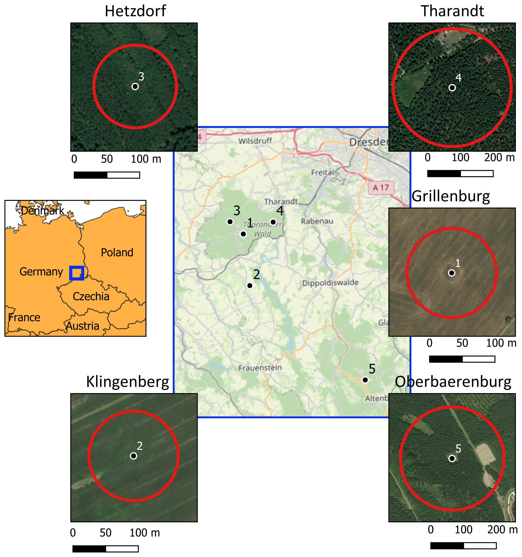
Figure 1 Location of chosen FLUXNET sites. Red circles represent footprints for each tower. OpenStreetMap (planet dump retrieved from https://planet.osm.org, last access: 20 November 2021) and Bing Satellite images (Bing Maps tiles, 2020) are used as a background.

Table 1 Short summary on the chosen FLUXNET sites.

2.2 BROOK90 model

BROOK90 (Federer et al., 2003) is a 1D process-oriented model for simulation of vertical water fluxes in soil–plant–atmosphere systems. Precipitation input (snow or rain) first goes through the canopy, where it could be intercepted and then evaporated. The portion, which reaches ground level, could be infiltrated, frozen, evaporated, converted to surface flow, percolated or stored as soil moisture. Infiltrated water follows a top-down approach as a macropore bypass and matrix flow. The soil column has groundwater, seepage and downslope outflow. Finally, soil water storage is used for evaporation and transpiration. The model has more than 100 physically based input parameters, but typically most are straightforward and can be set easily (as location or slope). As the study mainly reflects evaporation, this part of the model is described in more detail.

The model uses a two-layer version of Penman–Monteith (PM) equation by Shuttleworth–Wallace (SW) (Shuttleworth and Wallace, 1985) to estimate the potential evaporation (PE) separately for canopy and soil surface accounting for the surface energy budget and the gradient for the sensible heat flux respectively. Canopy-dependent PE consists of evaporation of intercepted snow and rain and plant transpiration. It is defined as the maximum evaporation that would occur from a given land surface under given weather conditions if all plant and soil surfaces were externally wetted. Surface-dependent PE includes evaporation from soil and snow surfaces. It is defined as the maximum evaporation that would occur from a given land surface under given weather conditions if plant surfaces were externally dry and soil water was at field capacity. The SW method considers multiple resistances like the above canopy, within canopy from canopy and ground, canopy surface, vapour movement in soil. They are applied in the standard PM equation, thus giving separate estimates of all five components of PE. It should be noticed, as BROOK90 distinguishes between soil and plant evaporation, that only one canopy process and one ground process can occur at a given time step. Subsequently, actual evaporation (E) is based on the water availability in the system (within the canopy, on the soil and within the soil matrix). Daily evaporation rates are calculated as a weighted sum of the daytime and nighttime values (based on the sunshine duration); however, interception could be estimated at a higher frequency (hourly).

Originally, the model was written in FORTRAN programming language; here we used an R “line-by-line” direct translated version (Kronenberg and Oehlschlägel, 2019).

2.3 Model frameworks and parameterization schemes

In the study, four different scale-dependent setups for the model are used to simulate evaporation and its components: Global BROOK90, EXTRUSO, BROOK90 with manual parameterization and calibrated BROOK90. To parameterize the model for global-, regional- and local-scale different topography, soil and land cover datasets were utilized. Most of the model's physical parameters are either default and thus fixed by the model developer or valid for whole model region (i.e. average duration of rain precipitation per month). Variable site-specific parameters (around 40 depending on the setup) and their values for all tested frameworks are listed in Appendix C (Table C1).

2.3.1 Global BROOK90 (GBR90)

The Global BROOK90 (GBR90) framework incorporates open-source global datasets for parameterization and forcing of the model using an R package (Vorobevskii et al., 2020). The main feature of the package is wrapping of the modelling process in a fully automatic mode based only on the location and time-interval input. The input area of interest is divided in a regular 50×50 m grid, and then hydro response units (HRUs) are identified based on the unique combinations of land cover, soil characteristics, and topography (aspect and slope). GBR90 provides fixed parameter sets for 20 land cover types based on Copernicus Global land Cover 100 m (Buchhorn et al., 2020): closed and opened forest (evergreen/deciduous, needle/broad leaf or mixed, and unknown), shrubs, herbaceous vegetation, moss and lichen, bare/sparse vegetation, cultivated and managed vegetation, urban territories and snow/ice. Additionally, leaf area index (LAI) and tall canopy height parameters were assigned using MODIS 8 d composite dataset with 500 m resolution (Myneni et al., 2015) and global forest canopy height with 30 m resolution (Potapov et al., 2021) respectively. The SoilGrids250 dataset (Hengl et al., 2017) provides global information on standard soil properties with 250 m resolution. Number of soil layers, stone fracture and profile depth parameters are directly derived from this dataset, while soil hydraulic parameters are assigned from the standard model developer's sets based on the derived USDA soil texture class. Amazon Web Service Terrain Tiles (Mapzen Data Products, 2020) are used as a provider for the global digital elevation model data (SRTM30 in the case of Saxony). The model is applied separately to each HRU, and an area-weighted mean is calculated. A more detailed description of the framework is presented in Vorobevskii et al. (2020).

2.3.2 EXTRUSO (EXTR)

The EXTRUSO (EXTR) is a semi-automatic framework for spatial water balance simulations on a regional scale (up to now only in Saxony, Germany) and is distributed via the R package (Luong et al., 2020). The HRU subset is also based on the overlay of soil and land cover types derived from the regional datasets. Due to specifics of these datasets (polygons rather than regular grid rasters), HRUs do not have regular dimensions. The framework has fixed parameterization for five land cover types (agriculture/cultivated land, deciduous forest, evergreen forest, grassland/meadows, urban/other territories). They are assigned according to the European land cover map CORINE 2012 (European Environment Agency, 2020) with 100 m resolution (some vegetation types from the map are generalized). Soil parameters are assigned similarly to GBR90, but using Saxon soil map BodenKarte50 (Sächsisches Landesamt für Umwelt, Landwirtschaft und Geologie, 2020) with 50 m resolution. The 10 m digital elevation model (Staatsbetrieb Geobasisinformation und Vermessung Sachsen, 2020) is used for slope and aspect estimates. As in GBR90, BROOK90 is run for each HRU and an area-weighted mean is stored. A full description of the framework is available in Luong et al. (2020).

2.3.3 BROOK90 (BR90) with “expert-knowledge” parameterization

Finally, we made a setup using the original BROOK90 model (BR90) with manual parameterization based on field measurements. These include long-term observations of the different canopy parameters conducted on the chosen FLUXNET sites (height, LAI, conductivity, albedo), soil profile data (soil texture, depth, stone fracture) and expert knowledge (i.e. interception parameters).

2.3.4 Calibrated BROOK90 (CBR90) as a benchmark

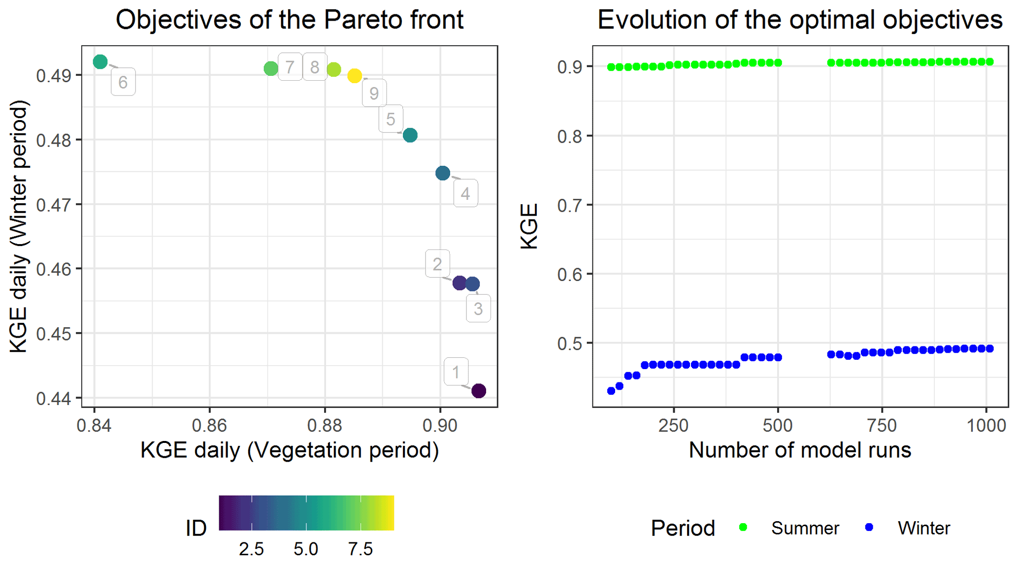
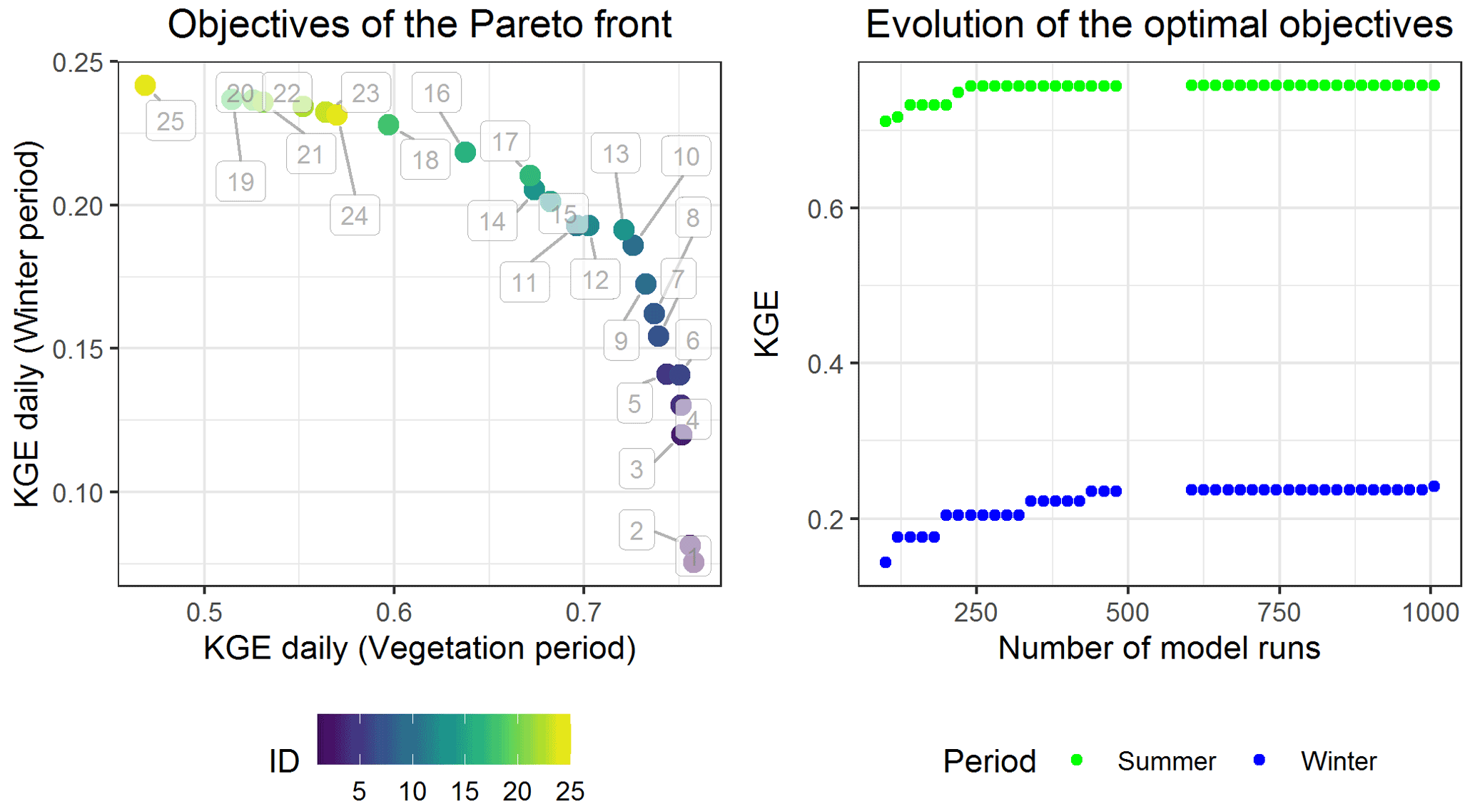
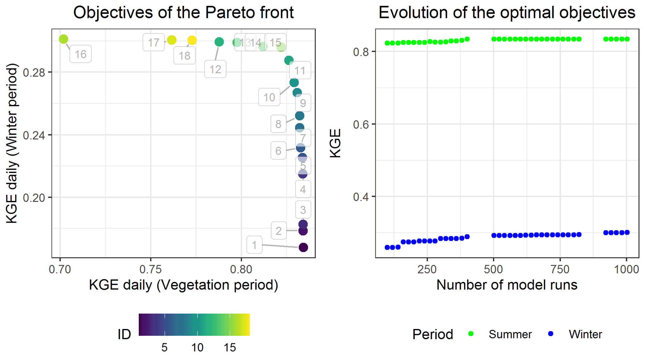
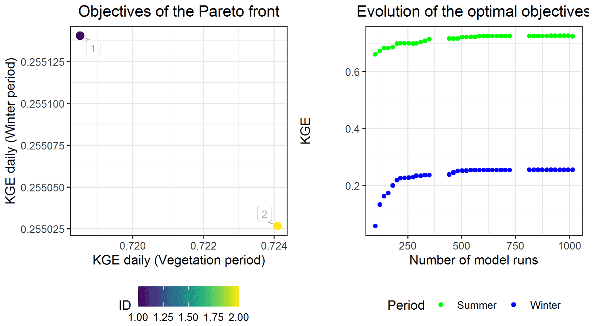
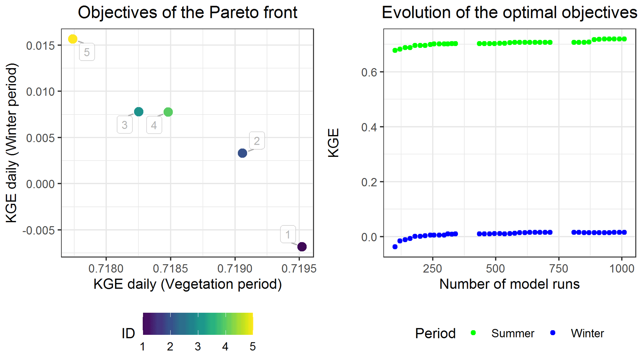
The calibrated BROOK90 (CBR90) serves as a benchmark for all other runs. For the calibration of BROOK90, we choose a multi-objective optimizer recently developed for the calibration of hydrological models. The algorithm is a hybrid of the MEAS algorithm (Efstratiadis and Koutsoyiannis, 2005), which uses the method of directional search based on the simplexes of the objective space and the epsilon-NSGA-II algorithm with the method of classification of the parameter vectors archiving management by epsilon dominance (Reed and Devireddy, 2004). Pareto-optimal solution was used to address two issues. First, as most of total annual evaporation occurs in the vegetation period, it makes sense to separate this period as the contribution of the winter months should have less “weight” during model fitting. Second we tried to account for possible systematic errors of eddy-covariance measurements themselves, which could vary significantly depending on the season (Hollinger and Richardson, 2005; Twine et al., 2000; Widmoser and Michel, 2021). Therefore the Pareto front could help to choose an optimal parameter set, namely enhancing winter month performance with insignificant loss of performance in vegetation period).

Here, we performed calibration and validation with a 70 %–30 % data split focusing on maximizing daily Kling–Gupta efficiency (KGE) values for total evaporation for the growing season (March–October) and the winter period (November–February). The initial parameter sets were set by “expert knowledge”. For the calibration we initially took the “location” parameters within a physically meaningful range, which are recommended by the developer and other researchers as the most sensible (Groh et al., 2013; Habel et al., 2021; Schwärzel et al., 2009; Vilhar, 2016). After the manual sensitivity analysis conducted using the given site-specific data, 21 parameters were chosen. In general, these include albedo, vegetation and flow characteristics. Meteorological forcing was derived from in situ measurements. The total number of trials was limited to 1000 model runs, which was sufficient to achieve stable performances for all three optimization functions.

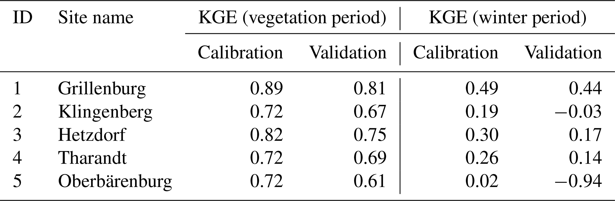
Results of the calibration and validation are presented in Table 2. A complete list of chosen parameters with given ranges and a graphical overview of the resulting Pareto fronts for each site are provided in Appendix C (Tables C1 and C2). The raw outputs of calibration results for all trials with optimized parameters can be found in the Supplement (Vorobevskii, 2021). It can be stated that calibration and validation showed satisfactory results for the vegetation period even on a daily scale, while the results for the wintertime were poor at most sites (more in detail in Sect. 4.2 and 4.3).

Table 2 Daily Kling–Gupta efficiency for BROOK90 calibration and validation.

2.4 Meteorological forcings

We have chosen ERA5 (Copernicus Climate Change Service (C3S): ERA5: Fifth generation of ECMWF atmospheric reanalyses of the global climate. ERA5 hourly data on single levels from 1979 to present, 2020), RaKliDa (Kronenberg and Bernhofer, 2015) and in situ station measurements to represent the global, regional, and local scales, respectively, as meteorological forcing for the model. The list of standard climatological variables required to run BROOK90 consists of minimum and maximum 2 m air temperature, mean 10 m wind speed, solar radiation on the horizontal surface, vapour pressure, and precipitation. Typically, daily data are required; however, if available, sub-daily precipitation data are more favourable.

ERA5 is a global climate reanalysis dataset from Copernicus and European Centre for Medium-Range Weather Forecasts, available from 1950 to near-real time at hourly resolution. It was derived using data assimilation principles by combining a global physical model of the atmosphere and observations from around the world. The original model resolution is 0.28125^∘, which corresponds to about 31×20 km rectangle in the area of interest. For the present study, data from the nearest to each site ERA5 grid were downloaded and processed by aggregating hourly to daily values.

RaKliDa is an open-source daily climatological dataset covering the south-eastern part of Germany (namely Saxony, Saxony-Anhalt and Thuringia) with a time span of 1961–2020. The original station data from the German Meteorological Service and the Czech Hydrological Meteorological Institute are first corrected for wind errors (Richter, 1995) and then interpolated on a 1×1 km grid using the Kriging indicator (Wackernagel, 2003). This approach is intended to reflect the orographic influence of downwind and upwind effects and to account for convective and small-scale precipitation events. As with ERA5, the nearest grid to each tower grid was used.

Daily meteorological data were taken from standard climate stations located in close proximity to the eddy-covariance towers. An exception is the wind speed, which is measured on the same height with eddy covariance. In addition, the available net radiation was assimilated above the canopy. Prior data analysis revealed up to 15 % of missing values (depending on location and variables). Since these values are generally not drastic, the majority of the missing parts fall within the model “warm-up” period, and the variance of the most problematic variable (wind speed) within a site is not very high; it was decided to fill the gaps with simple monthly averages.

All of the inputs required by BROOK90 are directly available in all three datasets, except for the vapour pressure, which was calculated using dew temperature data (Murray, 1967) for ERA5 and mean daily temperature with relative humidity for two others (Magnus formula).

The meteorological data prepared for BROOK90 can be found in Supplement (Vorobevskii, 2021). A graphical overview of the differences between three datasets is presented in Appendix A.

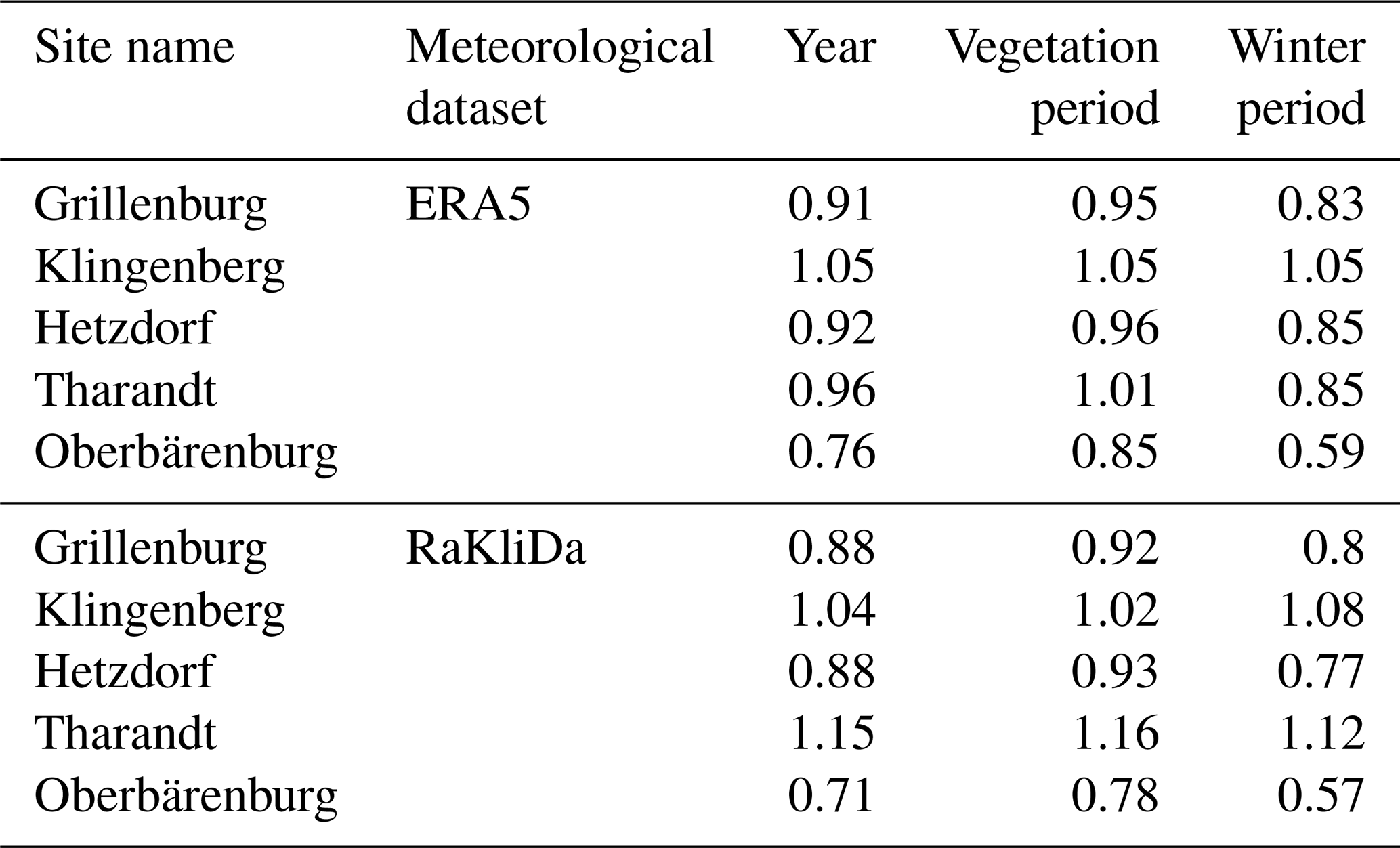
Of the six input meteorological variables, net solar radiation and precipitation have the biggest influence on evaporation. Global radiation in the gridded datasets showed minor but systematic overestimation compared to measurements on the mean daily scale (around 1 MJ m⁻² d⁻¹ in winter and 2–3 MJ m⁻² d⁻¹ in summer months). However, summer variations (peaks and minimums) are underestimated probably due to cloud coverage problems in ERA5 and RaKliDa. Precipitation showed a much larger and non-systematic difference between the three datasets. In general, higher mean daily precipitation was measured from September to March in Grillenburg, Hetzdorf and Tharandt (0.5–2 mm d⁻¹). However, when looking at the bias values (Table 3), a negative bias is typical for both datasets (except Klingenberg for both and Tharandt for RaKliDa). The behaviour of the vegetation and winter periods separately follows the annual bias. Temperature and available vapour pressure appear to be consistent, with 1–3^∘C and 0.01–0.03 kPa respectively variation from measurements in the summer months. The exception is Oberbärenburg, where the maximum temperature and available vapour pressure from ERA5 and RaKliDa have higher deviations, probably due to neglecting higher altitude in the datasets. Finally, wind speed possesses a systematic positive bias (1–2 m s⁻¹) for all months, except for ERA5 in forests and Klingenberg.

Table 3 Precipitation bias (to in situ measurements).

2.5 Evaluation of parameterization and forcings combinations

To assess the sensitivity of the BROOK90 to different parameter and meteorological inputs with regard to the evaporation simulations, we propose to create different combinations of the framework's parameterizations from global, regional and, local schemes and meteorological inputs from global, regional and local datasets (Fig. 2). Additionally, we tested the sensitivity of the setups to the temporal resolution of the forcing data (hourly and daily for ERA5).

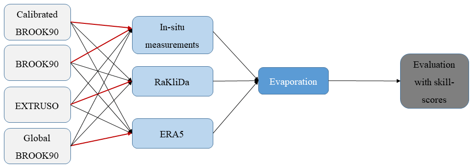
Figure 2 Principal scheme of the framework's mixture. Red arrows represent the original “parameter set–meteorological forcing” combination.

From the model runs, we extracted total evaporation and its five components: transpiration, evaporation of intercepted snow and rain, evaporation from soil, and snow evaporation. These results were evaluated on daily and monthly scales for the whole year and separately for the winter and vegetation periods using the following performance metrics: mean absolute error, Nash–Sutcliffe efficiency (NSE) (Nash and Sutcliffe, 1970) and Kling–Gupta efficiency (KGE) (Gupta et al., 2009). The last one can be decomposed into three main components important to assess process dynamics: correlation, bias, and variability errors. The formulas and optimal ranges for each performance metrics are listed in Appendix B.

Additionally, to test the uncertainty of the obtained performance, small data resampling experiment was designed (here only for the daily KGE values). It helps to show the possible performance spread due to general time-series shortage and occurrence of some extreme years (e.g. like wet 2003 and 2012 or dry 2018 and 2019). Thus, for each station we calculated multiple KGE values with reduced time-series length by randomly (1000 samples with replacement) throwing away 3 years of data (same for all cross-combinations). Obtained values serve to assess the possible KGE spread for each framework and meteorological dataset.

2.6 FAO grass-reference evaporation

To compare the relative complex BROOK90 model with other one, but at the same time remain on the same methodological background of Penman–Monteith equation, the FAO approach was chosen. The method is considered as a state of the art for grass-reference evapotranspiration estimations (Paredes et al., 2020; Sentelhas et al., 2010). Potential daily evaporation values are obtained on the basis or simplified Penman–Monteith approach (facilitation concerns aerodynamic and surface resistances calculations) with the radiation (shortwave and longwave), air temperature, wind speed and humidity as the input data (Allen et al., 1998).

3 Results

3.1 Daily and monthly total evaporation

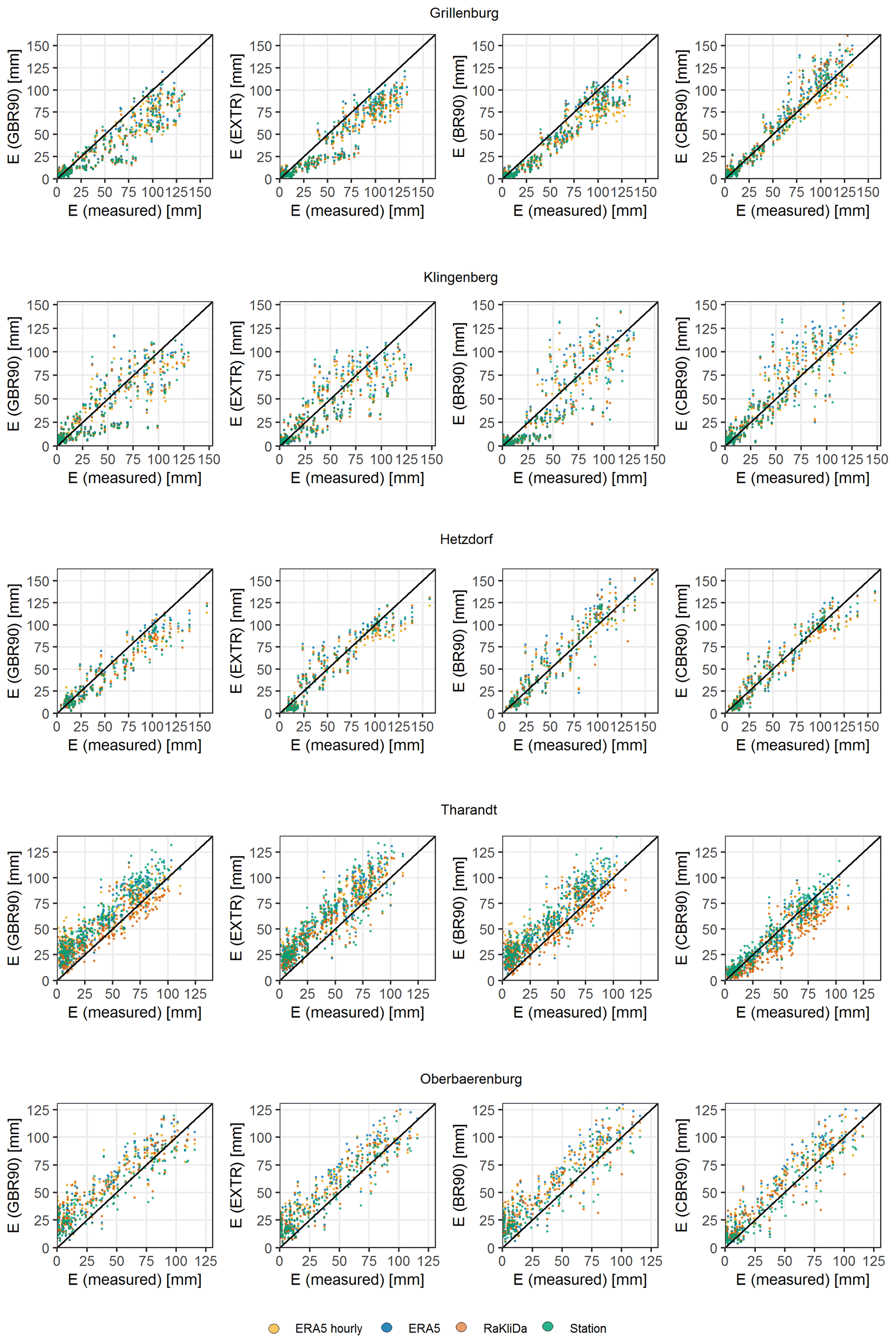
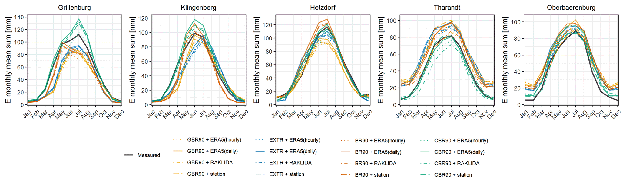
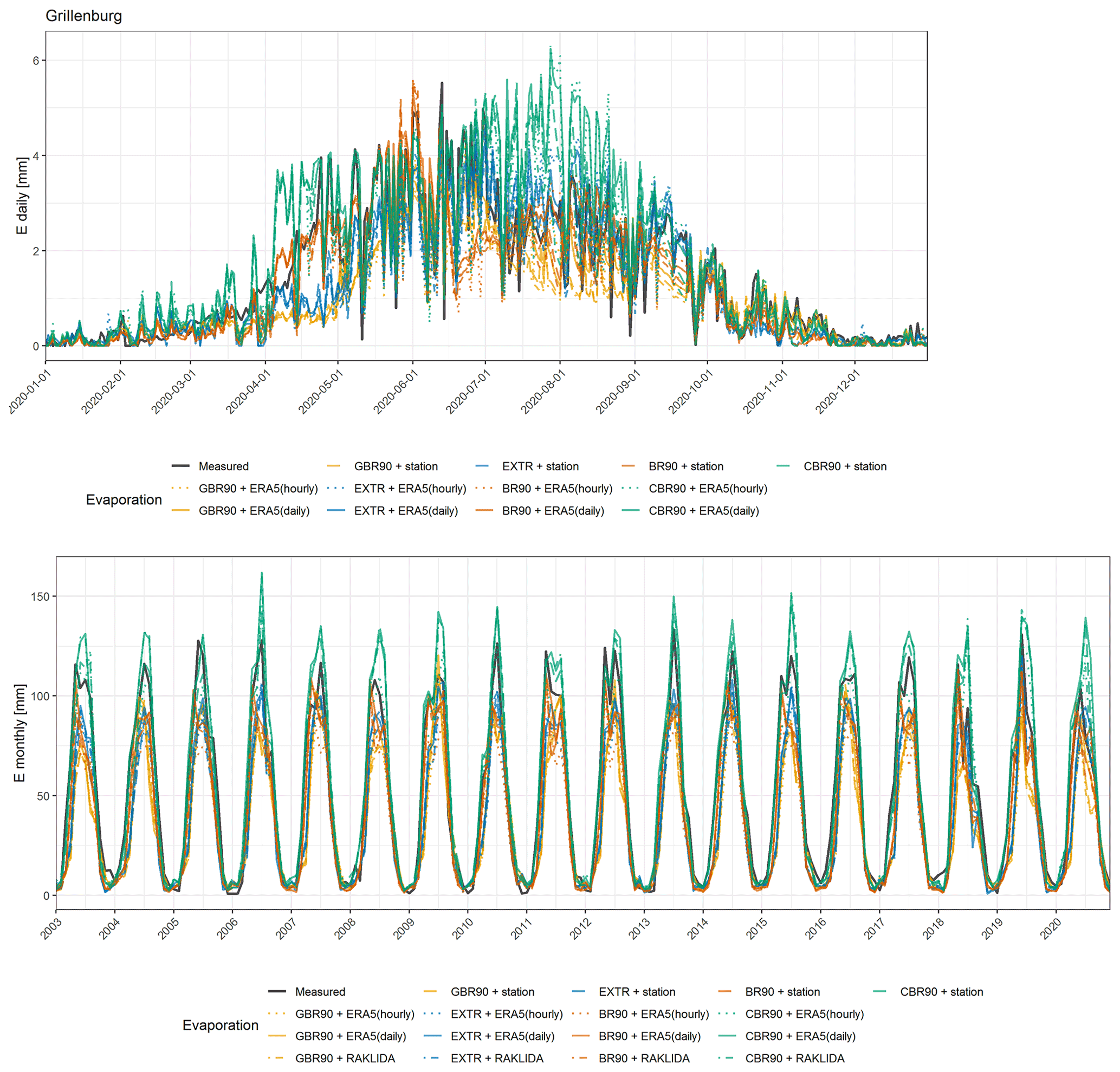
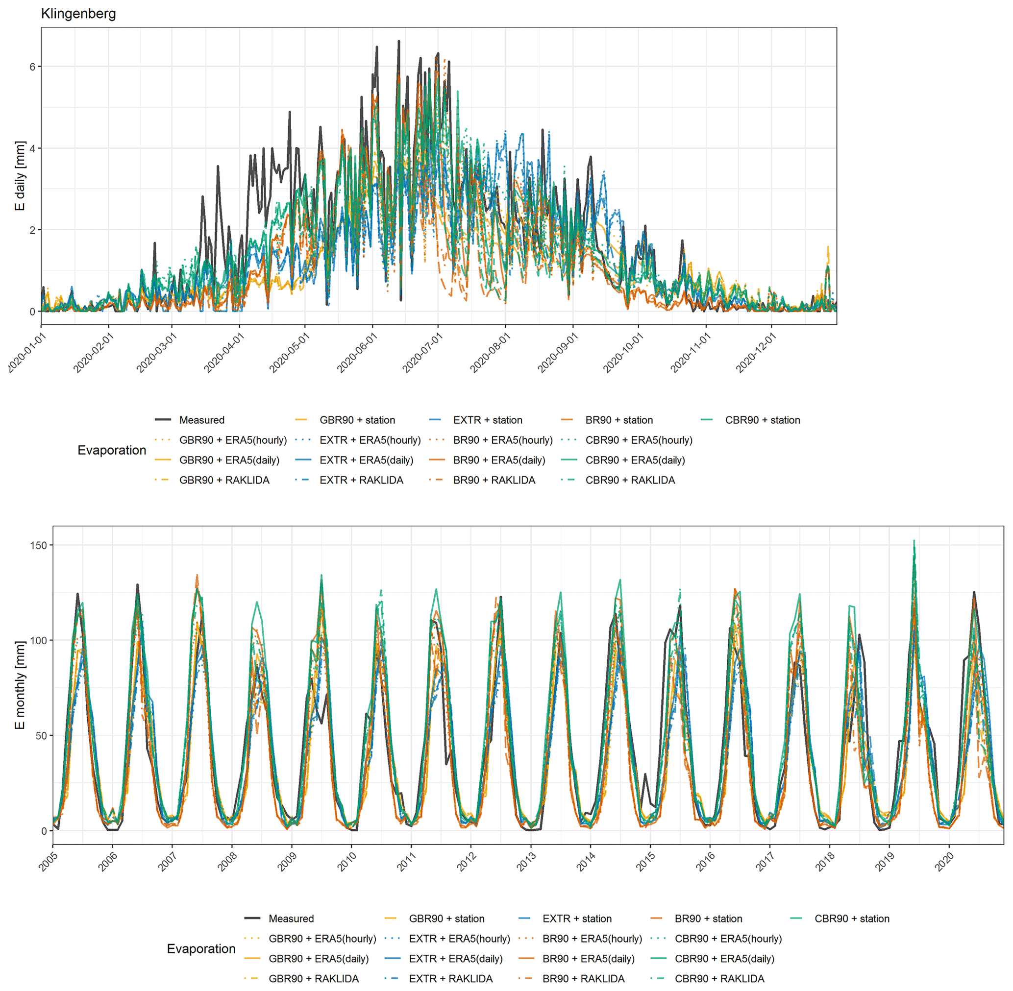
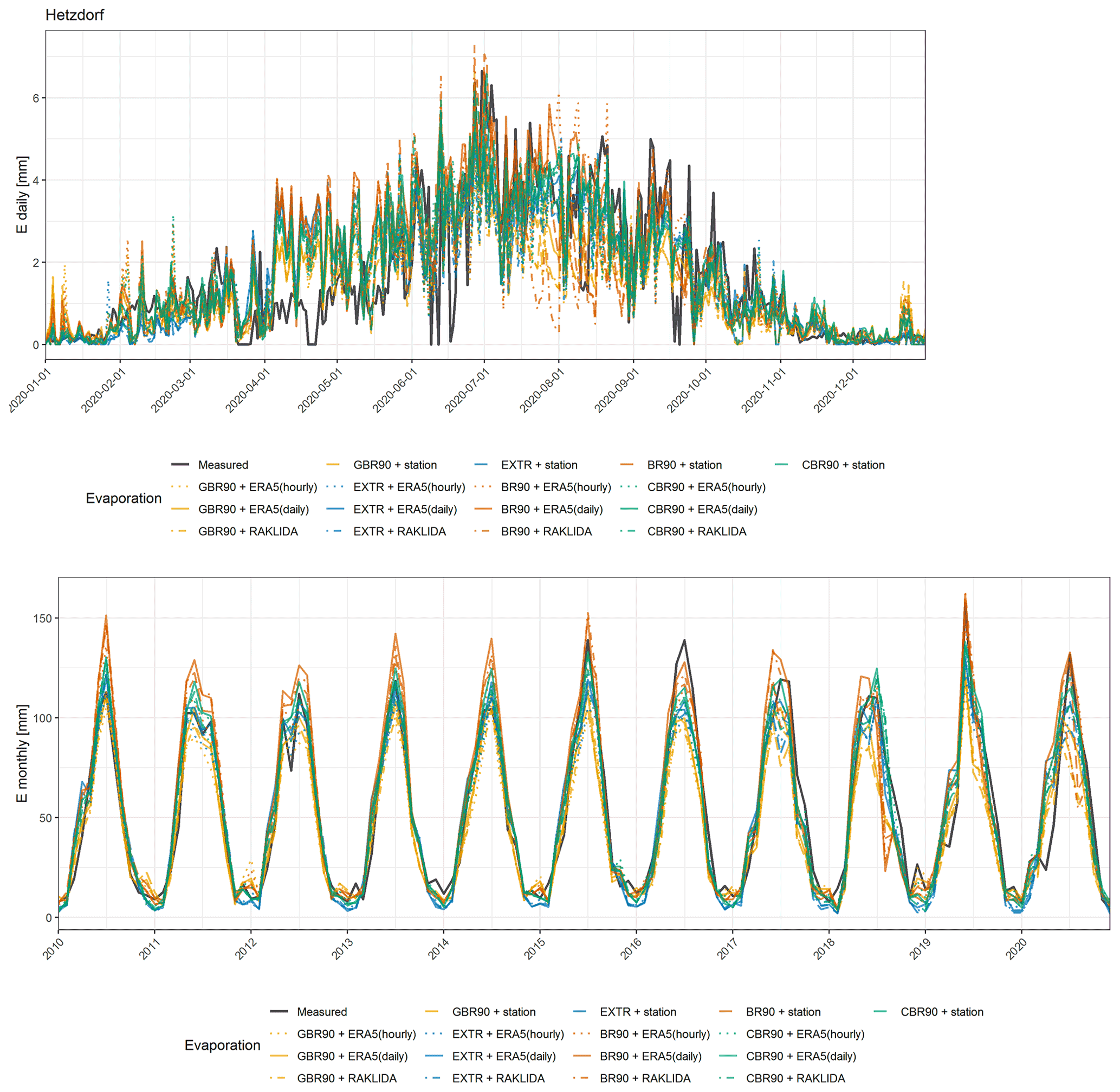
At first, a visual analysis of the modelled evaporation was performed. Therefore, daily (for 2020) and monthly (for the whole period with available measurements) time series (Appendix D), monthly quantile–quantile (Fig. 3) and mean monthly (Fig. 4) plots were analysed.

Daily evaporation of 0–0.5 mm in winter and up to 6–7 mm in summer months (with a maximum of about 10 mm) was found for the Grillenburg's grassland. All model setups showed similarly low values in November–February. The growing period (March–May) was represented with a delay of 3–4 weeks for GBR90 and EXTR and 2–3 weeks for BR90. Calibration helped to eliminate this time shift on a monthly scale, however at the same time enhancing the unreasonably high variability on a daily scale. During the summer months (June–August), the frameworks suffered from the systematic overestimation of variance ratio and underestimation of the mean values, which is especially noticeable within the higher evaporation values range. Moreover, monthly maximum values vary from year to year due to differences in the timing of grass cuts. Evaporation in autumn is well captured but advanced by 2–3 weeks in EXTR and BR90. Finally, the difference between meteorological datasets is only noticeable in the summer months.

In Klingenberg's crop field, evaporation of 0–1 mm in winter and 4–6 mm in summer months (with maximum around 9 mm) is usually observed. In most of the years, all model setups showed a similar small overestimation in November–January. It was relatively difficult to achieve a good model fit regarding the timing of the growing and harvesting periods even on a monthly scale, since the both periods of the various crops differ by up to two months and the annual rotation with clear cuts are irregular. The growing period (February–May) had in general a delay of 2–6 weeks. Here CBR90 shows higher daily evaporation values, thus fitting low bias, while the variation stays underestimated. In contrast with the grassland site, summer months (June–August) did not depict a high bias; the main problem appears in a considerable scattering due to poor correlation, which is higher in the middle part of Q–Q plot. Furthermore, the different setups showed different peak values in the summer months, BR90 matched observations in June, while GBR90 and EXTR showed the maximum in July. Finally, in autumn, none of the setups provided satisfactory results, namely both over- and underestimations, especially in September and October. Again, based on the meteorological datasets, the variability of the model performance is visible only in the summer months.

For the Hetzdorf deciduous broadleaf forest, typical values of winter and summer evaporation are 0–1 and 3–5 mm (with maximum around 8.5 mm), respectively. All model setups showed small amounts of evaporation in winter with a low bias, but also low correlation. The main leaf development period (March–May) was represented well by GBR90, with a 2–3-week time lag in April for EXTR and BR90. In the summer months (mostly in June and July) GBR90 and EXTR underestimated evaporation by 10 %, while “expert knowledge” BR90 gave positive bias. It can be noticed on the monthly plots that as the forest keeps developing and growing intensively within the last 10 years, higher evaporation rates were observed from year to year. At the same time due to model parameter stationarity, BR90 shows closer to the observed evaporation values only in the last 2 years. The annual mean monthly peak (July) and leaf fall were well captured by all models. Here the variance ratio reaches the closest to the optimum values in comparison to all the other sites. Only for the summer months, a rather small difference of about 10 mm per month between the meteorological forces could be captured.

In the evergreen coniferous forest of Tharandt, daily evaporation usually yields 0–0.3 mm in winter and 2–3 mm in summer (with maximum around 7 mm). All setups except CBR90 demonstrated a high bias for the seasons (15–20 mm per month), which is larger in winter, where daily peaks are sometimes as high as summer maximums. Moreover, the inter-annual variability appears to be highly overestimated as well. Like for the grassland, the model calibration reduced the mean error to optimum values, but the problem of daily peaks in winter remained unsolved. In contrast to the other sites, a noticeable difference between forcings can be observed (up to 10 % in the summer months) with the in situ measurements delivering the highest evaporation amount.

The evergreen coniferous forest of Oberbärenburg normally has evaporation rates of 0–0.3 mm in winter and 2–3 mm in summer (with maximum around 8 mm). Evaporation here is 5 %–10 % higher in the growing season than at the Tharandt site. Still, most of the setups (except in spring and CBR90) showed a positive bias, which is higher in winter and July. Similar to Tharandt, winter daily peaks sometimes exceeded summer extremes. Here, even the calibrated model did not demonstrate a good agreement in general and did not remove winter overestimations. Oberbärenburg was the only site where the well-known European drought of 2018 is clearly visible on a monthly scale. The data show around 30 % less evaporation in summer months due to depletion of the soil water and overall precipitation deficit. However, most of the model setups did not depict this effect properly. Finally, the spread between meteorological datasets here is not as broad as for the Tharandt site.

Figure 3 Observed and modelled monthly evaporation values for all setups.

Figure 4 Observed and modelled monthly mean evaporation values for all setups.

In Fig. 5, the daily KGE values are shown, while the monthly results and other criteria (NSE, MAE) are presented in Appendix E. Based on KGE values, a good agreement was found between all model setups and observations for all the sites (Fig. 5). The best agreement showed the combination “CBR90 +  station data” (from 0.72 in Oberbärenburg to 0.91 in Grillenburg) and the worst “GBR90 +  hourly ERA5” (from 0.36 in Grillenburg to 0.71 in Hetzdorf). On the monthly scale, all setups demonstrated higher performance, which is approximately 5 % better than on the daily scale. The goodness of fit in the vegetation period was better and very similar to the whole year, while the performance in wintertime for all setups was lower, resulting sometimes in negative KGE values (down to −0.6). Here BR90 and EXTR showed poor agreement with the observations in the fields (Grillenburg and Klingenberg) and in the deciduous forest (Hetzdorf) respectively.

With a few exceptions, the best performance among the meteorological datasets was achieved for the station data and daily ERA5. On average for all the five sites, in terms of KGE values, the spreads in the meteorological forcings yielded 0.09 (maximum of 0.17 showed BR90 for Grillenburg), while scattering in the parameterization schemes was much higher and yielded 0.25 (with the maximum of 0.54 for Grillenburg and in situ meteorological data).

Finally, KGE spreads calculated for each combination from a resampled time series are generally small. On the annual scale and for the vegetation period, higher uncertainties of obtained KGE values were found in Grillenburg, Klingenberg and Hetzdorf (10 %–15 % on average), while in Tharandt and Oberbärenburg KGE deviations were low (around 5 %). For the winter months, the spread possessed the same behaviour but resulted in much higher values (up to 100 %). Among all the frameworks, GBR90 was associated with the largest uncertainty on the annual scale in almost all the cases, while it had the smallest spread in the winter, where uncertainty of EXTR and BR90 dominated.

NSE values are in general similar to KGE, but slightly smaller, which range from − 0.05 for GBR90 in Grillenburg and Oberbärenburg to 0.88 for CBR90 with station data. Mean average errors vary from 0.39 up to 0.98 mm d⁻¹ with the highest values in evergreen forests for GBR90 and the lowest in Grillenburg for CBR90.

The hourly resolved ERA5 data did not produce better results, showing the worst performance on the annual scale in most cases.

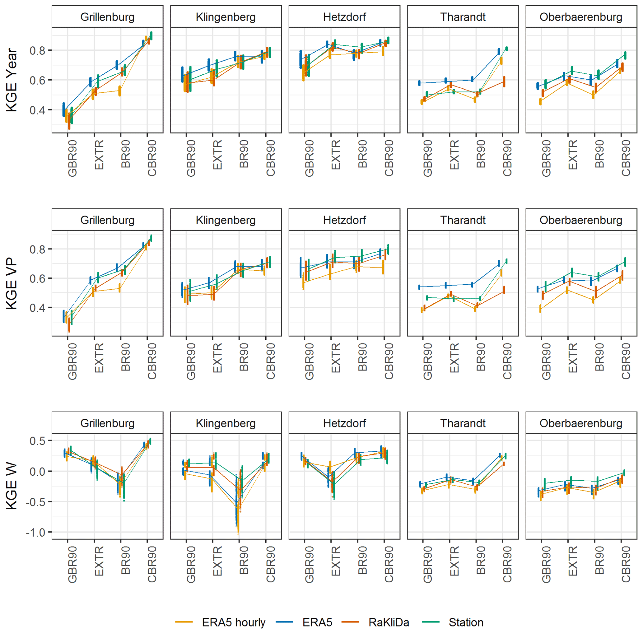
Figure 5 KGE values for daily evaporation: whole year, vegetation and winter periods. Vertical lines for each cross-combination refer to bootstrapped KGEs.

The major advantage of the KGE criteria is the possibility to obtain a deeper understanding of model performance through its decomposition. A closer look at the KGE components (Fig. 6) reveals that correlation coefficients for the fields (Grillenburg and Klingenberg) and deciduous forest (Hetzdorf) are relatively high for all model setups (0.75–0.95), and the main problems occur in underestimation of the mean (0.7–0.8) and variability ratios (0.55–0.7) (except for BR90 in Hetzdorf). In general, there are only small fluctuations between model forcings for these three sites. In evergreen forests, on the other hand, the correlation showed much higher spread among both parameterizations and meteorological datasets (0.4–0.75). Furthermore, bias and variability ratios possess, on the other hand, significant positive deviations from the optimal values (except variability in Oberbärenburg), especially in Tharandt (up to 1.6). Overall, ERA5 and station data perform better than others in most of cases. The hourly ERA5 forcing did not show a noticeable difference in evaporation bias or variability, but reduced correlation in the forests (by 5 %–15 %). Finally, it could be noticed that in comparison to the other setups, CBR90 brings bias and variance ratio almost to 1, but it did not improve correlation for all the sites (i.e. Hetzdorf).

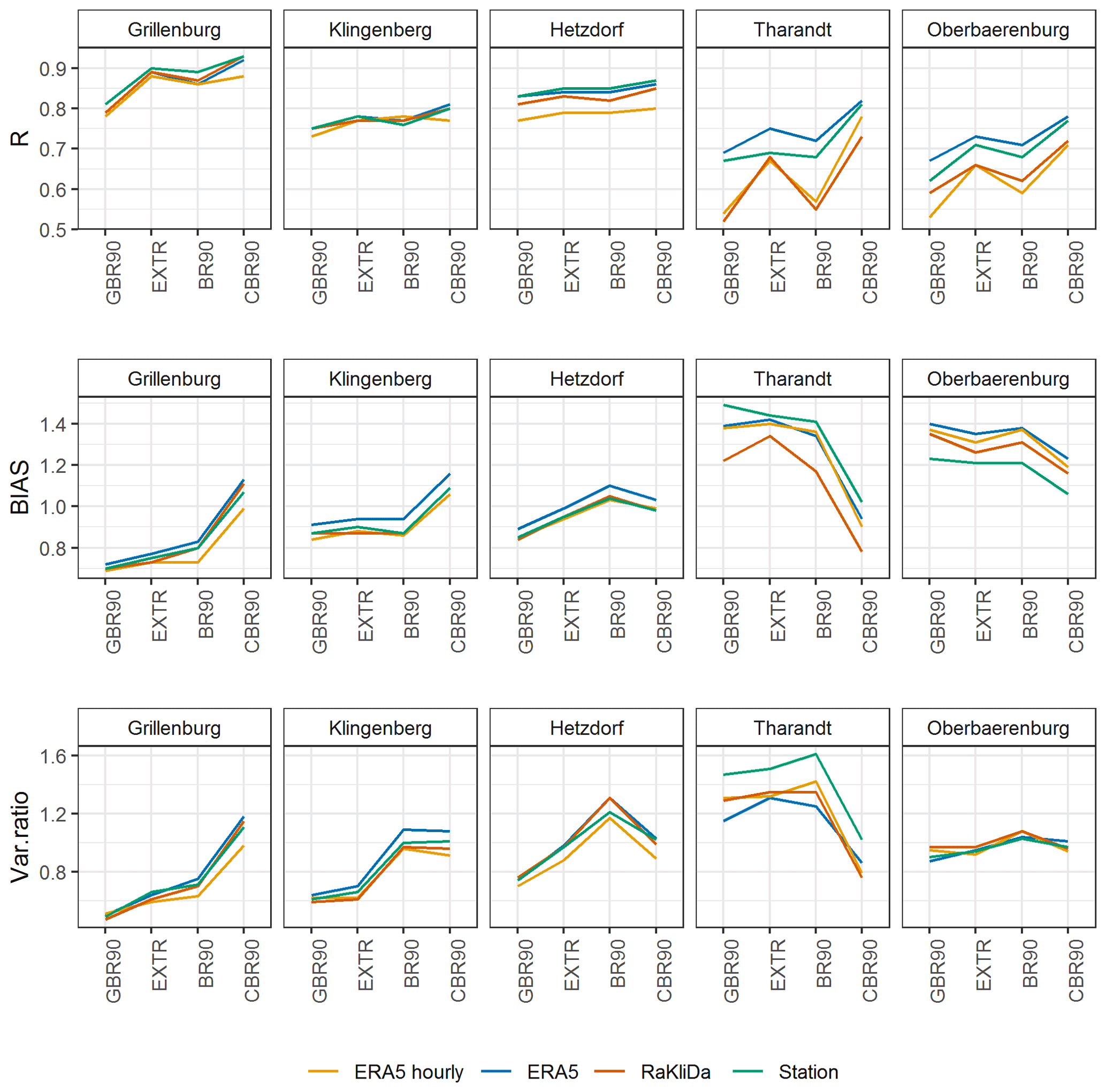
Figure 6 Decomposition of KGE for daily evaporation for the whole year: correlation, bias and variance ratio.

3.2 Evaporation components

The 40 %–60 % partitioning between total flow and evaporation components in global terrestrial water balance (Müller Schmied et al., 2016) also applies to the BROOK90 point simulations. With a variation in mean annual precipitation from 877 mm (Klingenberg) to 1141 mm (Oberbärenburg), measured mean annual evaporation varies from 476 mm (Tharandt) up to 625 (Hetzdorf) mm. This leads to measured E–P ratios of 0.41 to 0.65, with the lowest values observed in old spruce forest and the highest in grassland and growing deciduous forest. Here, both the global and regional frameworks showed an overestimation of the ratio for the evergreen forests (Tharandt and Oberbärenburg) and an underestimation for the fields (Grillenburg and Klingenberg) (can be found in the Supplement, Vorobevskii, 2021).

Summarized annual evaporation components (averaged from all tested model setups) are presented in Fig. 7. According to this figure, transpiration in fields and deciduous forest yields 68 %–73 %, and evergreen forest transpires about 58 %–59 %. In Tharandt and Oberbärenburg 31 %–35 % of precipitation goes to interception (mainly rain, interception of snow is less than 2 %). In Grillenburg, Klingenberg and Hetzdorf evaporation of the intercepted precipitation is lower and yields 14 %–23 %. Soil evaporation, on the other hand, is higher in the fields (11 %–15 %) and lower in forests (4 %–8 %). Evaporation from snow is less than 2 % at all sites. The vegetation period spans 8 months in total and accounts for most of the annual evaporation (85 %–95 %). Thus, the distribution of components is generally consistent with a slightly higher contribution from transpiration. In winter, evaporation consists mainly of interception in forests and soil or snow evaporation of the fields.

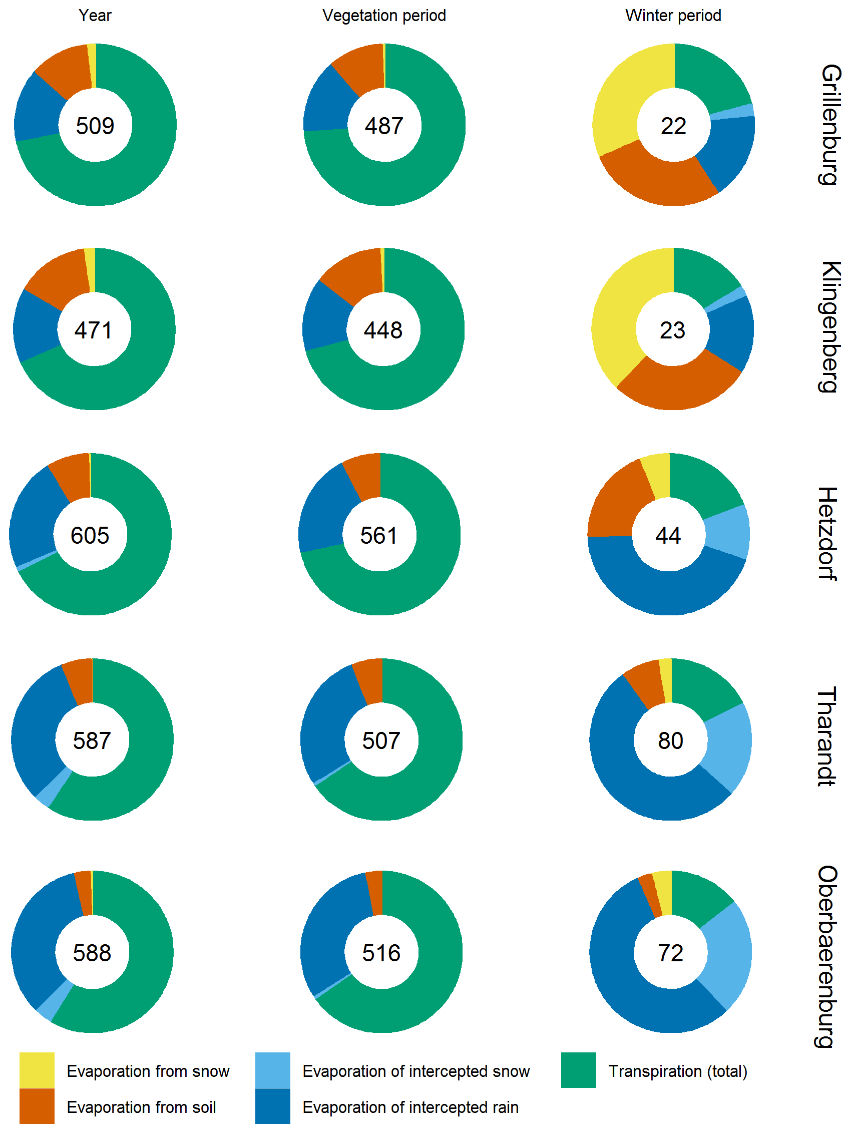
Figure 7 Mean annual and seasonal evaporation components averaged over all model setups. The numbers inside pie charts refer to the mean evaporation sums per year or season.

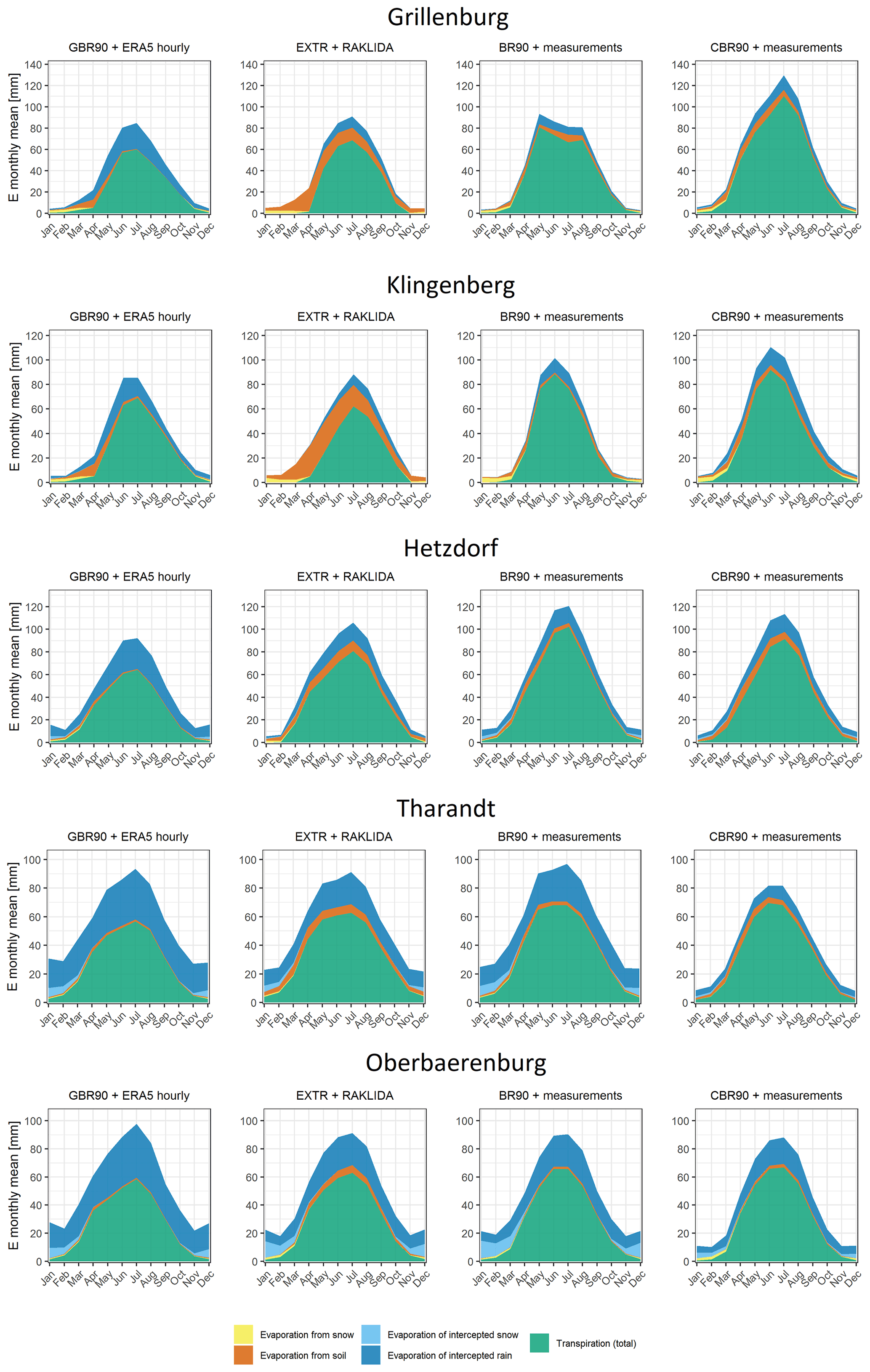
To get more insights on the possible setups' differences regarding the evaporation partitioning, we show “natural” model parameterization and forcing combinations (Fig. 8). Only minor differences were observed in evergreen coniferous forests. This mainly concerns intercepted rain. GBR90 with hourly ERA5 shows the largest amount (40 %–68 %) and CBR90 with station data reduces interception up to 15 %–30 %, which is especially noticeable in Oberbärenburg. At the other three sites, seasonality plays a bigger role in the redistribution of evaporation components. Indeed, in the fields, almost no interception was modelled in EXTR using RaKliDa and BR90 with station data in winter and early spring, and all evaporation in these months consists of snow and soil evaporation. Furthermore, the transpiration is dominant in summer and autumn times with sharper edges due to crop and grass cutting. In general, EXTR delivers more soil evaporation than other model setups, while GBR90 produces more rain interception. Slightly smoothened but similar results could be observed in the deciduous forest of Hetzdorf. Since the actual distribution of the components is unknown, we can only assume that CBR with in situ meteorological data indicates conditions that are the closest to reality. Considering this, we can rank the goodness of the framework in the evaporation representation in the following order (best to worst by similarity to CBR90): BR90, EXTR, and GBR90, which seems indeed logical.

Figure 8 Modelled mean monthly evaporation components.

3.3 Grass-reference evaporation: comparison of BROOK90 and FAO model with measurements

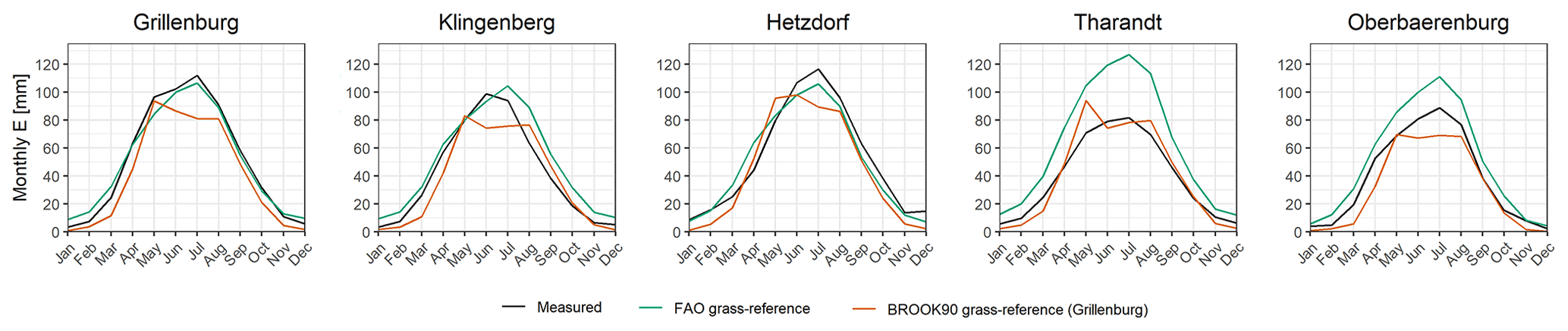
A comparison of the FAO “potential” and BROOK90 “actual” grass-reference evaporation output is presented in Fig. 9. For that, in the BROOK90 model the original site-specific vegetation parameters were replaced with “grassland” ones from Grillenburg manual parameterization scheme. Station meteorological input data were considered for both approaches.

FAO estimations of field sites (Grillenburg and Klingenberg) showed a good fit with the observed data, except a time lag of 1 month on the autumn time and minor overestimations of evaporation in wintertime (5–10 mm per month). BROOK90 simulations possess a noticeable time lag of a 2–3 weeks in spring periods and underestimated the evaporation in spring and summer months up to 20 %.

Minor variances of around 10 mm per month between FAO and measured evaporation could be seen in the deciduous forest of Hetzdorf, namely a small overestimation in spring period and an underestimation in summer months. Actual grass-reference evaporation from BROOK90 simulations, on the other hand, was lower than eddy-covariance measurements for all months, except April and May.

In evergreen forests FAO depicted considerably higher potential grass-reference evaporation than was observed throughout the whole year, but especially in summer months (up to 30 %–40 % in July). BROOK90 did not show high systematic deviations from the observations in Tharandt (except the peak in May), while in Oberbärenburg simulated evaporation was systematically lower for all months (especially in summer time).

Figure 9 Observed and modelled monthly mean grass-reference evaporation.

4 Discussion

4.1 Role of the framework's spatial scale in parameterization and forcing

The comparison of GBR, EXTR and BR90 frameworks showed how the model is sensible to the scale of the setup with regard to evaporation. Moreover, coupled with the fact that CBR90 showed significantly higher performance than other setups for almost all the sites, it was indirectly confirmed that the model is more sensible to the scale of parameterization scheme rather than to the scale meteorological forcing. However, these conclusions need to be backed up with the assumption that both meteorological data and parameters used for each spatial scale come from state-of-the-art sources. Thus, they are both representative and possess the best quality (currently) for global, regional and local scales respectively.

Analysis of the parameters used in the study and their ranges revealed which groups of them demonstrated the most noticeable influence on the accuracy of evaporation simulations and are at the same time affected by the scale of the model setup (Appendix C, Table C1).

At first, the plant leaf parameters must be highlighted, namely albedo, LAI and height, and interception storages. Surface reflectivity with and without snow regulates the net radiation and thus directly affects potential evaporation. The values generally have a wide range of 0.1–0.3 for vegetation and 0.2–0.9 for snow, and their estimations are subject of high uncertainties (Alessandri et al., 2020; Myhre and Myhre, 2003; Page, 2003; Park and Park, 2016; Wang et al., 2017). Here they were assigned with global and regional studies for GBR90 and EXTR respectively, while for BR90 measured values were used. Maximum LAI and its seasonal cycle are probably the most sensible and uncertain parameters in the model regardless vegetation type, while plant height and its seasonality plays a greater role and is more uncertain for the short (grass and cropland), rather than in tall (forest) canopies. These two parameters often control the biggest portion of potential evaporation (transpiration and interception) as well as its partitioning (Hoek van Dijke et al., 2020; Wegehenkel and Gerke, 2013; Yan et al., 2012). Here global scale was represented with remote-sensing estimates, while regional and local scale use fixed values from regional studies and expert knowledge, which apparently showed better results for the case study. The interception storage and intercepted precipitation fraction are the key parameters for the correct estimation of interception amount (Wu et al., 2019). They are all plant-, season- and age-dependent and possess high variability, which makes it very challenging to generalize their values for the vegetation classes (Federer and Douglas, 1983; Leaf and Brink, 1973; Pypker et al., 2005; Yang et al., 2019). In all frameworks they are set up as the default or with expert knowledge. Nevertheless, only due to these parameters, the interception uncertainty could be as high as ±20 mm per month, especially in forests.

The second group denotes to soil parameters. Soil structure, profile depth and coarse fragment's fraction directly determine the maximum water storage capacity for the site. Here, the scale plays a crucial role, since the quality of available datasets decreases drastically from local to global scale due to the scarcity of soil profile data and very high heterogeneity of soils (REF). Soil hydraulic properties certainly have a big influence on the water retention and holding capacity, controlling water supply for the actual soil evaporation and transpiration (Carminati and Javaux, 2020; Lehmann et al., 2018; Verhoef and Egea, 2014). However, the scale uncertainty due to this parameter group is difficult to assess, since these parameters are assigned indirectly based on sand, silt and clay content for each layer and fixed parameter set. Thus, the problem is narrowed to correct identification of the soil texture, which is still a challenging task even for a regional scale (Hengl et al., 2017).

Significant difference in the model performance due to different meteorological input datasets was not evident for all setups and sites (bootstrapped values in Fig. 5). Here, the spatial scale did not follow the main hypothesis, as the global dataset ERA5 was not the worst and in many cases outperformed in situ meteorological data. It would appear that the RaKliDa dataset with its 1 km spatial resolution could fit the eddy-covariance footprint at least as good as station data; however, it sometimes demonstrated the worst performance or close to hourly ERA5. This outcome contradicts the generally accepted application of regional meteorological forcings to simulate evaporation in high resolution (Martens et al., 2018; Rudd and Kay, 2015; Wang et al., 2015; Zink et al., 2017). However, probably due to location peculiarities of the study sites, and good agreement of the global reanalysis with station data, the regional dataset did not show competitive performance. Namely, ERA5 showed slightly better precipitation bias values than RaKliDa (Table 3). Moreover, RaKliDa exhibits a systematic underestimation of the global radiation, especially in the summer months (Appendix A).

4.2 Challenges in the model process representation

Although BROOK90 has a decent physically based representation of the evaporation process, it shows some limitations as well. At first, BROOK90 treats the vegetation as a single layer (big leaf). Thus, the complexity of canopy vertical structure is omitted, which can be insignificant for simple ecosystems like meadows or cropland, but it can play a big role in multi-layered vegetation (Bonan et al., 2021; Luo et al., 2018; Raupach and Finnigan, 1988). For example, lack of undergrowth representation could have a significant effect on the evaporation underestimation in forests with a dense floor like Hetzdorf. Additionally, there is no allowance for non-green leaves, which intercept precipitation and radiation but in the meantime do not transpire. This process can play a role in deciduous forests like Hetzdorf in autumn and winter, as they generate too much transpiration. Furthermore, since the phenomenon of ground frost is not considered, soil evaporation is not limited on these days, which could lead to a substantial overestimation in winter. As canopy parameters are assumed constants, phenology or growth (e.g. crop rotation in Klingenberg and continuous forest growth in Hetzdorf) as well as drought affecting LAI (reduction due to prolonged water stress) are not considered in the model. Snowpack energy and evaporation modules suffer from overestimations in tall canopies; thus an arbitrary reduction factor is applied. Finally, albedo does not depend on solar elevation angle, canopy structure, or snow age. These limitations alone could have a substantial influence on total evaporation and its timing.

In addition, the PM equation uses vapour pressure deficit and net energy as the main factors to calculate potential evaporation. The first variable is derived directly from the daily input temperature and available vapour pressure using the Magnus equation and does not vary much between different methods (Lide, 2005). For net energy, the situation is different. The shortwave radiation is an input and its net value is controlled by the rather vague albedo, while the longwave radiation is estimated internally using the effective emissivity of the clear sky. Under these assumptions, the potential discrepancy between different formulas can be as high as 20–30 W m⁻². After obtaining a persistent positive bias for evaporation in the forests, we checked the energy balance of the model with in situ measurements (Fig. 10). In fact, minor differences were found for all input datasets. In the summer period, minor overestimation was found for ERA5 and station data in Grillenburg, Klingenberg and Tharandt and underestimates for RaKliDa in Hetzdorf and Tharandt. In winter (especially in December and January), large relative underestimation was discovered in Grillenburg, Hetzdorf and Oberbärenburg. Therefore, with a negative amount of energy, BROOK90 still showed higher monthly evaporation than measured. Specifically, according to Fig. 8, 90 % of the actual evaporation in forests in winter consists of interception, and normally there is no absence of precipitation input during this period. Because of the peculiarities of the PM approach, positive potential evaporation can be estimated with negative net energy, positive vapour pressure deficit, and low estimated atmospheric and canopy resistances. Thus, as long as vapour pressure deficit exists, the evaporation flux tries to fill the gradient.

Figure 10 Observed and modelled monthly mean net energy on canopy and ground level.

Finally, as it was found, the hourly resolved input precipitation data did not produce better results, showing the worst performance (hourly ERA5 data) on the annual scale in most cases. This brings up the question of reliability of the subdaily calculations in BROOK90 interception module, i.e. which omits diurnal cycle of potential evaporation and consistently produces too much interception if hourly input is used (Federer, 2002). However, it could also be the quality of subdaily precipitation distribution in the ERA5 data for the study region, since on daily, monthly and annual scales ERA5 did not show a significant difference with the station data, which could account for high differences in daily and hourly performance.

4.3 Reliability of eddy-covariance measurements

Reliability of the evaporation measurements with eddy-covariance technique themselves is a widely discussed question. Standard methods of the “energy-balance-closure” corrections (Wilson et al., 2002; Richardson et al., 2012) do not always lead to necessary bias adjustment (Foken, 2008; Imukova et al., 2016). Therefore, largest systematic deviations between observed and modelled evaporation, which could be discussed in the context of inaccuracy of the measurements, were discovered in the evergreen forests in winter, in grassland in summer and in pasture in growing season. Analysis of the evaporation components and comparison of the FAO with the BROOK90 grass-reference evaporation helped to reveal some discrepancies in the eddy-covariance measurements.

The time lag during the growing and harvesting periods for Klingenberg could be explained with permanent crop rotation and inability of FAO and BROOK90 models to cope with non-stationarity in vegetation parameters. Overestimation in winter for the FAO method for both sites could be a result of simplifications of FAO-modified PM equation against SW approach in BROOK90 (i.e. neglecting the soil water-holding capacity). According to the continuous long-term measurements of grass height in Grillenburg, regular grass cutting is performed in June–July. This in general should lead to evaporation decline, which can be seen clearly in Fig. 4 for monthly evaporation of BR90. However, this effect was not found in the measurements (even on a daily scale). Moreover, mean evaporation usually shows maximum annual values in July. Besides possible systematic measurement errors, this could be explained by an underestimation of the real site footprint. Another explanation is near-saturation conditions of the soils. Thus, there is an almost unlimited water supply and perturbation of the evaporation components after grass cutting (drastic increase of soil evaporation). Nevertheless, while calibrating the model, it was realized that it is impossible to increase soil evaporation by almost 30 mm during the summer months and to stay within the physically meaningful boundaries for soil parameters for the given soil profile. The findings are consistent with other studies, where latent heat fluxes were systematically over- and underestimated depending on the season in in short canopies (Moorhead et al., 2019; Perez-Priego et al., 2017; Twine et al., 2000).

In Tharandt and Oberbärenburg FAO approach showed 10–20 mm evaporation in the winter months, while BROOK90 resulted in 3–5 mm (consisting only of soil and snow evaporation). At the same time, all model setups showed 20–30 mm of evaporation per month in winter (which consists of more than 80 % intercepted precipitation), while only 5–10 mm is observed. Thus, it is possible that the interception is generally underestimated by eddy-covariance measurements in the forests. Moreover, while the calibration in Tharandt helped to adjust the simulated evaporation in winter months as well (primarily by increasing the winter albedo), in Oberbärenburg even a relatively wide parameter range was not sufficient. Here, the large variations between two approaches emphasize the importance of the soil and in a regulation of the evaporation, since different soil types appear at the grassland and evergreen forest sites (Gleysols and Podzols respectively). As few researchers pointed out, the reliability of eddy-covariance data within the rainy days and when the interception dominates is indeed questionable (Dijk et al., 2015; Wilson et al., 2001).

In addition, a previous analysis of eddy-covariance data for some of the study sites showed that the possible under- and overestimations in measurements could be as large as ± 8 %–11 % for Tharandt, ± 29 %–36 % for Grillenburg and ± 28 %–44 % for Klingenberg (Spank et al., 2013).

Therefore, in addition to reliability of the mean net energy and precipitation (Sects. 2.4 and 4.2), it is possible that the quality of the eddy-covariance data is questionable due to at least systematic underestimation of interception and non-representative footprint.

5 Conclusion and outlook

This study presents the qualitative analysis and discussion of the BROOK90 model scale uncertainties with regard to evaporation simulations. We tried to answer the question of how the model setup scale influences the performance and whether the model is more sensitive to the parameter set or to the meteorological input. For this, three frameworks (Global BROOK90, EXTRUSO and BROOK90 with manual parameterization) and three forcing datasets (ERA5, RaKliDa, in situ measurements) were used, representing the global, regional and local scale, respectively. We made cross-combinations of them and model evaporation components for five locations in Saxony, Germany, covered by long-term eddy-covariance measurements: grassland (Grillenburg), cropland (Klingenberg), deciduous broadleaf forest (Hetzdorf) and two evergreen needleleaf forests (Tharandt, Oberbärenburg).

Our results indicated that all setups perform well even on a daily scale, with KGE values ranging from 0.35–0.80. KGE decomposition demonstrated that with high correlation coefficients in grassland, cropland and deciduous forest, performance was affected here mainly by bias and variance ratios, whereas in evergreen forest all three components varied greatly. The highest and lowest values among all setups were achieved by the same combination of Global BROOK90 and ERA5 in Hetzdorf and Grillenburg respectively. Calibration of the model helped to increase KGE significantly, especially for Grillenburg and Tharandt. The vegetation period where 90 %–95 % of the total annual evaporation is observed, showed much higher agreement with the observations than the winter period.

The main finding of the study is that, for all tested setups, parameterization gave us approximately 4 times higher spread in model performance than meteorological forcings for all sites. Furthermore, while the difference in parameter sets mattered throughout the year, the difference in the meteorological datasets was evident only in summer months. Analysis of the breakdown of evaporation components revealed that in the vegetation period transpiration yields up to 65 %–75 % of total evaporation, while in the winter months interception (in forests) and soil/snow evaporation (in fields) play a major role. Moreover, different parameter sets show substantial differences in the redistribution of evaporation components. Finally, the discussion questioned the meteorological data quality, limitations of the model and reliability of the eddy-covariance measurements.

In the outlook, we would like to suggest possible future directions on this topic:

• Expand the number of study sites with other FLUXNET towers.

• Run a similar analysis for other physically based models.

• Analyse model uncertainty by incorporating runoff and soil moisture in the analysis.

• Apply and validate different methods to breakdown eddy-covariance data in components.

Appendix A: Comparison of BROOK90 meteorological input data (ERA5, RaKliDa and station measurements)

Figure A1 Monthly daily mean meteorological variables.

Figure A2 Daily values of meteorological variables for 2020.

Appendix B

Table B1 Skill scores.

Appendix C: BROOK90 main parameters and calibration results

Table C1 Main site-specific parameters (topography, coil and land cover related) used in tested BROOK90 frameworks. SAI – stem area index.

^* for GBR90 and EXTRUSO listed parameters denote the dominant HRU.

Table C2 BROOK90 parameters and their ranges chosen for the calibration.

Abbreviations for ranges: G – Grillenburg, K – Klingenberg, H – Hetzdorf, T – Tharandt, O – Oberbärenburg.

Figure C1 Resulted calibration Pareto fronts for Grillenburg (chosen ID – 9).

Figure C2 Resulted calibration Pareto fronts for Klingenberg (chosen ID – 13).

Figure C3 Resulted calibration Pareto fronts for Hetzdorf (chosen ID – 15).

Figure C4 Resulted calibration Pareto fronts for Tharandt (chosen ID – 2).

Figure C5 Resulted calibration Pareto fronts for Oberbärenburg (chosen ID – 5).

Appendix D: Daily (2020) and monthly (whole time series) simulations

Figure D1 Grillenburg.

Figure D2 Klingenberg.

Figure D3 Hetzdorf.

Figure D4 Tharandt.

Figure D5 Oberbärenburg.

Appendix E: Evaluation of the simulated evaporation

Table E1 Daily evaporation skill scores for the whole year.

Table E2 Daily evaporation skill scores for the vegetation period.

Table E3 Daily evaporation skill scores for the winter period.

Table E4 Monthly evaporation skill scores for the whole year.

Table E5 Monthly evaporation skill scores for the vegetation period.

Table E6 Monthly evaporation skill scores for the winter period.