the Creative Commons Attribution 4.0 License.
the Creative Commons Attribution 4.0 License.
 | 21 Jun 2022
Morphological controls on surface runoff: an interpretation of steady-state energy patterns, maximum power states and dissipation regimes within a thermodynamic framework
Samuel Schroers
Olivier Eiff
Axel Kleidon
Ulrike Scherer
Jan Wienhöfer
Erwin Zehe
Recent research explored an alternative energy-centred perspective on hydrological processes, extending beyond the classical analysis of the catchment's water balance. Particularly, streamflow and the structure of river networks have been analysed in an energy-centred framework, which allows for the incorporation of two additional physical laws: (1) energy is conserved and (2) entropy of an isolated system cannot decrease (first and second law of thermodynamics). This is helpful for understanding the self-organized geometry of river networks and open-catchment systems in general. Here we expand this perspective, by exploring how hillslope topography and the presence of rill networks control the free-energy balance of surface runoff at the hillslope scale. Special emphasis is on the transitions between laminar-, mixed- and turbulent-flow conditions of surface runoff, as they are associated with kinetic energy dissipation as well as with energy transfer to eroded sediments. Starting with a general thermodynamic framework, in a first step we analyse how typical topographic shapes of hillslopes, representing different morphological stages, control the spatial patterns of potential and kinetic energy of surface runoff and energy dissipation along the flow path during steady states. Interestingly, we find that a distinct maximum in potential energy of surface runoff emerges along the flow path, which separates upslope areas of downslope potential energy growth from downslope areas where potential energy declines. A comparison with associated erosion processes indicates that the location of this maximum depends on the relative influence of diffusive and advective flow and erosion processes. In a next step, we use this framework to analyse the energy balance of surface runoff observed during hillslope-scale rainfall simulation experiments, which provide separate measurements of flow velocities for rill and for sheet flow. To this end, we calibrate the physically based hydrological model Catflow, which distributes total surface runoff between a rill and a sheet flow domain, to these experiments and analyse the spatial patterns of potential energy, kinetic energy and dissipation. This reveals again the existence of a maximum of potential energy in surface runoff as well as a connection to the relative contribution of advective and diffusive processes. In the case of a strong rill flow component, the potential energy maximum is located close to the transition zone, where turbulence or at least mixed flow may emerge. Furthermore, the simulations indicate an almost equal partitioning of kinetic energy into the sheet and the rill flow component. When drawing the analogy to an electric circuit, this distribution of power and erosive forces to erode and transport sediment corresponds to a maximum power configuration.
- Article
(4632 KB) - Full-text XML
-
Supplement
(148 KB) - BibTeX
- EndNote


Surface runoff in rivers and from hillslopes is of key importance to biological, chemical and geomorphological processes. Landscapes, habitats and their functionalities are coupled to the short- and long-term evolution of rainfall–runoff systems. As we live in a changing environment, it has been of major interest to explain the development of runoff systems and how ecological (Zehe et al., 2010; Bejan and Lorente, 2010), chemical (Zhang and Savenije, 2018; Zehe et al., 2013) and geomorphological (Leopold and Langbein, 1962; Kirkby, 1971; Yang, 1971; Kleidon et al., 2013) processes are organized in time and space. Here we focus on the energy balance of surface runoff, particularly at the hillslope scale, using a thermodynamic framework. Typically, the momentum balance of surface runoff and streamflow is strongly dominated by friction, which is usually characterized by the flow laws of Darcy–Weißbach, Manning or Chezy (Nearing et al., 2017). Consequently, hydraulic estimates of flow velocities rely on the semi-empirical parameters of these laws, which in essence express the ability of a system to dissipate free energy via friction into heat and thus to produce entropy (Zehe and Sivapalan, 2009). A thermodynamic perspective appears hence as the natural choice for deeper understanding of how the mass, momentum and energy balances of surface runoff are controlled by and interact with the landscape and how short- and long-term feedbacks determine the co-development of form and functioning of hydrological systems (Paik and Kumar, 2010; Singh, 2003).
1.1 Thermodynamics in landscape evolution and optimal channel networks
Leopold and Langbein (1962) were among the first to introduce thermodynamic principles in landscape evolution. Representing a one-dimensional river profile as a sequence of heat engines with prony brakes (see Fig. 1), they showed that the most likely distribution of potential energy per unit flow along a river's course to the sea follows an exponential function. Their main hypothesis was that streamflow performs the least work or, equivalently, that the production of entropy per flow volume is constant. Yang (1976) extended this principle and termed it minimum stream power and detailed how flow velocity, slope, depth and channel roughness of a stream should adjust to minimize stream power. In his work about optimal stream junction angles, Howard (1990) also assumed that stream power is minimized, while Rodriguez-Iturbe et al. (1992) proposed that optimal channel networks (OCNs) minimize overall energy dissipation. The authors postulated three principles: (1) the principle of minimum energy expenditure in any link of the network, (2) the principle of equal energy expenditure per unit area and (3) the principle of minimum total energy expenditure in the entire network. Subsequent work of these authors (Rodriguez-Iturbe et al., 1994; Ijjasz Vasquez et al., 1993) revealed that application of these principles yielded three-dimensional drainage networks in accordance with Horton's laws of stream number and stream lengths (Smart, 1972).
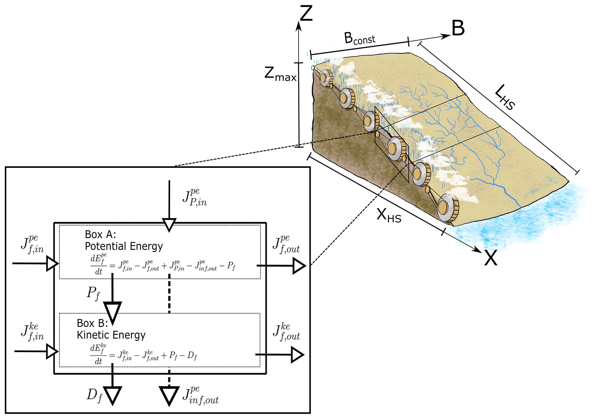
Figure 1Hillslope open thermodynamic system with spatial division into a sub-OTS as a two-box open thermodynamic system. Each control volume (sub-OTS) is represented by a prony brake (compare Leopold and Langbein, 1962).
In climate research, Paltrigde (1979) proposed the principle of maximum entropy production. He showed that a simple two-box model allowed for a successful reproduction of the steady-state temperature distribution on Earth, which maximizes entropy production, expressed as the product of the heat flow and the driving temperature difference. Kleidon et al. (2013) argued that maximum entropy production in steady state is equivalent to a maximization of power, which means that the flow extracts free energy at a maximum rate from the driving potential energy gradient. The authors applied the maximum power principle to river systems and proposed that they develop to a state of maximum power in sediment flows: while the driving geopotential gradient is depleted at the maximum rate, the associated sediment export maximizes at the same rate. Furthermore, the authors relate maximum power in the river network to minimum energy expenditure, as minimum dissipation implies that a maximum of potential energy can be converted into kinetic energy of the water and sediment flux.
1.2 Surface runoff and hillslope morphology and the role of energy conversions
Though surface runoff on hillslopes is governed by the same physics as streamflow, there are also important differences. Overland flow is an intermittent threshold response to rainfall events (Zehe and Sivapalan, 2009), caused either by infiltration excess (Horton, 1945; Beven, 2004) or saturation excess (Dunne and Black, 1970). Surface runoff flows along a partially saturated soil and may hence either accumulate downslope or re-infiltrate. Downslope re-infiltration implies an export of water mass and thus potential energy into the soil (Zehe et al., 2013), and the related decline in flow depth reduces shear stress, which affects the momentum balance. Overland flow is typically very shallow compared to the roughness elements, which makes the use of the above-mentioned flow laws even more challenging (Phelps, 1975), and it manifests either as diffusive sheet flow or advective flow in rill networks. Due to the transient nature of overland and sediment flows, rill networks are generally transient, but they develop in a self-reinforcing manner (Gómez et al., 2003; Rieke-Zapp and Nearing, 2005; Berger et al., 2010). Micro rills emerge at some critical downstream distance on the hillslope (compare the “belt of no erosion” in Horton, 1945) and continue in parallel for some length before they merge into larger rills (Schumm et al., 1984). Sometimes these rills split apart before converging into larger gullies (Achten et al., 2008; Faulkner, 2008) and finally connecting to a river channel. This transitional emergence of a structured drainage network was firstly stated in Playfair's law (cited in Horton, 1945) and has since then been observed in a variety of studies (Emmett, 1970; Abrahams et al., 1994; Evans and Taylor, 1995). Motivated by the similarity to river networks and surface rill networks, several experimental studies explored whether rill networks grow towards and develop as least-energy structures in accordance with the theory of optimal channel networks (Gómez et al., 2003; Rieke-Zapp and Nearing, 2005; Berger et al., 2010). The studies of Rieke-Zapp and Nearing (2005) and Gómez et al. (2003) revealed that the emergence of rill networks and their development implies indeed a reduction of energy expenditure, which has previously been shown for stream channel networks (Ijjasz Vaquez et al., 1993). In line with these findings, Berkowitz and Zehe (2020) proposed that rill flow reduces the volume specific dissipative energy loss due to a larger hydraulic radius compared to sheet flow, which is equal to smaller rills merging into a larger one, as noted by Parsons et al. (1990).
The possible optimization of river or rill network geometries through the interplay of surface runoff, erosion and deposition of soils/sediments is the first point that motivates an analysis from a thermodynamic perspective. The second point relates to the transition from laminar- to turbulent-flow conditions, which was already corroborated by Emmet (1970) in a set of comprehensive field and laboratory experiments to investigate hydraulics of overland flow. As laminar flow converts more potential energy into kinetic energy per unit volume than turbulent flow, it is of interest whether and how this transition relates to the emergence of rills and their optimization. Parsons et al. (1990) measured the hydraulic properties of overland flow on a semiarid hillslope in Arizona and attributed the observed downslope decrease in the frictional flow resistance to the accumulation of surface flow in fewer but larger rills. This is similar to a transition of inter-rill flow, from here onwards referred to as sheet flow (Dunne and Dietrich, 1980), to rill flow. More recently a concept emerged that upholds a theory of a slope–velocity equilibrium (Govers et al., 2000; Nearing et al., 2005), claiming that physical and therefore hydraulic roughness adapts such that flow velocity is a unique function of the overland flow rate independent of slope.
1.3 Objectives and hypotheses
In the light of this concise selection of studies, we propose that an energy-centred perspective on overland flow on hillslopes might be helpful to better understand the co-evolution of hillslope form and functioning and whether those (and other) hydrological systems evolve towards a meta-stable, energetically optimal configuration (Zehe et al., 2013; Kleidon et al., 2014; Bejan and Lorente, 2010). Following the work of Kleidon (2016), we develop the general thermodynamic framework and explain how surface runoff along rivers and hillslopes fits into this setting (Sect. 2). We argue that despite the similarity of hillslope surface runoff and river runoff, morphological adaptations and the related degree of freedom of both systems manifest at distinctly different scales. Mature river elements are mainly fed by the upstream discharge and local base flow, while hillslope elements receive substantial water masses during runoff events through local rainfall and upslope runon. This causes an interesting trade-off along the overland flow path, where mass grows downslope due to flow accumulation, while geopotential height declines. We hypothesize that these antagonistic effects lead to a peak in potential energy of overland flow at a distinct point on the hillslope. This implies an upslope area, where the potential energy of overland flow is growing due to flow accumulation (though water is flowing downslope) before it starts declining in downslope direction. From a thermodynamic perspective, the ability of surface runoff to perform work increases up to the point of maximum potential energy and is then depleted through a cascade of energy conversion processes. Our second hypothesis is, thus, that this build-up of potential energy occurs under laminar flow conditions with a low degree of freedom for morphological changes, while the location of potential energy maximum coincides with the emergence of turbulent flow and with a maximum degree of freedom for morphological changes, including the emergence of rills.
The first application of our framework tests hypothesis 1, by exploring how typical shapes of hillslope topography in combination with different width functions control the spatial patterns of potential and kinetic energy of surface runoff and energy dissipation along the flow path during steady states (Sect. 3). As these shapes represent different morphological hillslope stages (Kirkby, 1971), shaped by erosive forces of previous surface runoff events (Rieke-Zapp and Nearing, 2005), we expect differences in the energy balance, including the location of the potential energy maximum. The second application of our framework tests hypothesis 2 (Sect. 4), by analysing the energy balance of surface runoff observed during hillslope scale rainfall simulation experiments in the Weiherbach catchment (Scherer et al., 2012). The experiments provide measurements of eroded sediments and total runoff including sheet and rill flow velocities at the lower end of the irrigated stripes and therefore present an opportunity to explore how rills and rill networks affect the energy balance of surface runoff. For that purpose, we calibrated an extended version of the Catflow model (Zehe et al., 2001), which accounts for the transition from sheet to rill flow, to these experiments and analysed the spatial patterns of potential energy, kinetic energy and dissipation with respect to the transition from laminar to turbulent flow based on simulated flow depths and velocities.
2.1 Free-energy balance of hillslopes as open thermodynamic rainfall–runoff systems
To frame surface runoff processes into a thermodynamic perspective, we define the surface of a hillslope as an open thermodynamic system (OTS; Kleidon, 2016). In this sense, the hillslope exchanges mass, momentum, energy and entropy with its environment (Fig. 1). Rainfall adds mass at a certain height and thus free energy in the form of potential energy along the upper system boundary. Mass and free energy leave the system at the lower boundary due to surface runoff or via infiltration as subsurface flow (Zehe et al., 2013). To express energy conservation of surface runoff, we start very generally with the first law of thermodynamics in the following form:
Equation (1) states that a change in the internal energy U (joules) of a system consists of change in heat H in joules plus the amount of work W in joules performed by the system. Here, the performed work dW remains part of the internal energy, as in an open environmental system work is usually performed in the system and does not leave it, as is the case for heat engines (Kleidon, 2016). Note that the capacity of a system to perform work is equivalent to the term “free energy”. Solving Eq. (1) for the change in free energy/work reveals hence that a change in heat is associated with a dissipative loss of free energy and production of thermal entropy. The latter reflects the second law of thermodynamics, which states that entropy is produced during irreversible processes. The free energy of surface runoff at any point on the hillslope corresponds to the sum of its potential and kinetic energy if we neglect pressure work (i.e. assuming constant pressure) and mechanical work (i.e. no shaft work such as pumps and turbines).
We apply Eq. (1) to balance both potential and kinetic energy of surface runoff separately and subdivide the hillslope into lateral segments along the horizontal flow path x (Fig. 1), with a given width b, and express energy fluxes in watts per metre (W m−1). Note that differences between in- and outflux of free energy in a hillslope element imply that these are either converted into another form of free energy or are dissipated. The potential energy balance of surface runoff depends on the topographical/geopotential elevation of the hillslope element, on the corresponding mass inputs due to rainfall and upslope runon, on the mass losses due to infiltration and downslope runoff, and on the energy conversion into kinetic energy (Eq. 2). In our notion, potential energy of infiltration excess surface runoff is converted into kinetic energy of overland flow, while kinetic energy is partly dissipated via friction into heat (Eq. 3), and another part is transferred into erosion and sediment transport. Note that in our two-box scheme (Fig. 1), we consider total energies of fluid flow (mean velocity, though possibly turbulent), and the kinetic energy balance residual Df does not separate energy transfer to sediments from frictional dissipation. We can thus write the potential and kinetic energy balance equations for any segment of the hillslope in watts per metre (Table 2):
Fluxes with superscript “pe” or “ke” relate to potential energy and kinetic energy, respectively. The subscript “f” relates to surface runon and runoff, subscript “inf” to infiltration and subscript “P” to precipitation (see Table 2). Equations (2) and (3) balance changes of potential energy of runoff and its kinetic energy , also expressed in terms of the net energy fluxes across the segment boundary , , . Pf is the transfer from potential to kinetic energy, and Df summarizes the frictional dissipation rate and the work needed for sediment detachment and transport as well as energy that is used to generate turbulent kinetic energy. While dissipation means free energy is lost as heat, kinetic energy transfer to the sediment is not dissipated, as it creates macroscopic motion. Along similar lines, one could separate turbulent kinetic energy from kinetic energy of the mean flow when including turbulent velocity fluctuations. By combining Eqs. (2) and (3), the total free-energy balance of a hillslope segment becomes
The change in total free energy of overland flow in a segment is equal to the sum of net energy fluxes minus dissipation. In the case of the steady state , the dissipation term Df can be determined as the residual of the steady-state energy balance. Before we further elaborate on this in Sect. 2.3, we reflect on the relation between the energy balance residual, frictional dissipation and the related flow laws.
2.2 The energy balance residual Df and frictional dissipation at the hillslope scale
Here, we focus on conversion of potential energy into kinetic energy because the former controls the hierarchy of possible energy conversion in surface runoff. We neglect the subsequent kinetic energy transfer to sediments and turbulent velocity fluctuations and refer to Df simply as the dissipation of kinetic energy. The concept could be extended to account for phase transitions from laminar to turbulent flow as well as for kinetic energy transfer to eroded sediment particles. In these cases, Df needs to be separated into the energy fluxes that (a) convert kinetic energy of mean flow into turbulent kinetic structures, (b) transfer energy to sediment motion and (c) dissipate free energy into thermal heat, while at the same time one needs to include the energy balance of eroded sediments.
For laminar flow, the downslope accumulation of runoff leads to a steeper vertical velocity gradient, which might surpass a critical threshold Reynolds number to create turbulent-flow structures (expressed as the relation of inertia to viscous forces). These convert kinetic energy of the mean flow into kinetic energy of small-scale velocity fluctuations and thereby reduce the kinetic energy and thus velocity of the mean flow. Turbulence in turn provides the power and force to detach and lift sediment particles, which also need to be accelerated (in the simplest case) to the mean flow velocity. Both erosion processes feed again on the kinetic energy of the mean flow, while particle detachment also feeds on the kinetic energy of raindrops. In the light of these thoughts, one can expect Df to be larger for turbulent than for laminar flow, when using the mean flow velocities to calculate , and Df should also be larger in the case of erosion and sediment transport. Both processes extract kinetic energy and consequently reduce mean flow velocities, as corroborated by Ali et al. (2012) for energy transfer to sediments in experiments of runoff on erodible beds. This energy transfer has implications for the inverse estimate of roughness coefficients from rainfall simulation experiments (also for those we use in Sect. 4). The important point to stress here is that in general an increase in an observed (apparent) resistance to flow due to a reduced mean flow velocity can but must not necessarily imply that a larger frictional dissipation is the underlying cause.
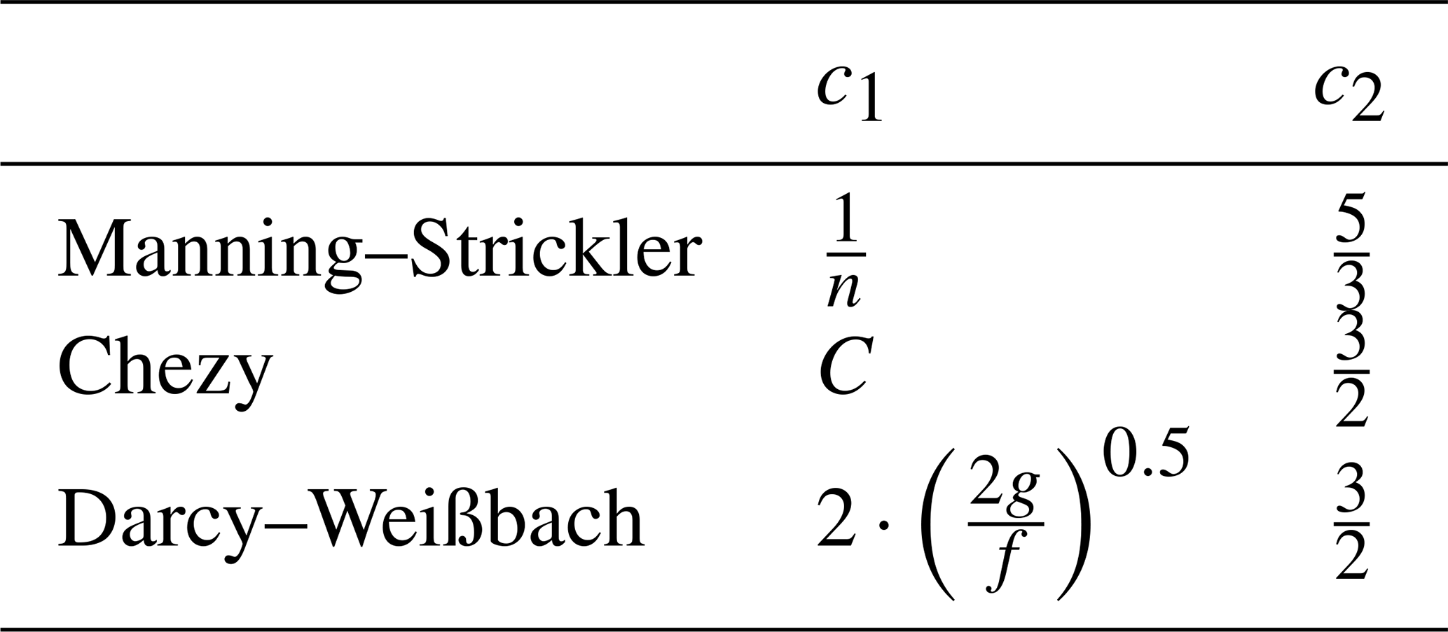
Govers et al. (2000) summarize the methods which are still in use today for estimating how frictional dissipation controls steady-state runoff velocities as a function of roughness, essentially representing the degree of free-energy loss from the mean flow. Most approaches focus on the generalization of a friction coefficient in time and/or space for a given surface area where runoff occurs, which is expressed by a general friction law that relates unit width discharge q to flow depth d and topographic slope S:
where c1 and c2 are coefficients, which vary for Manning–Strickler (Manning's n), Chezy (C) and Darcy–Weißbach (f) (Singh, 2003, Table 1).
Although it is known that friction coefficients on hillslopes vary with the degree of roughness element inundation (Lawrence, 1997) and sediment transport concentrations and are transient (Abrahams et al., 1994), mean flow velocities are in practice estimated using constant values. Without additional information about the flow regime and transport process, these coefficients provide, as explained above, an uncertain estimate of frictional energy dissipation of free energy into heat and related entropy production (Govers et al., 2000). Furthermore, experiments by Govers (1992) for rill flow as well as by Nearing et al. (2017) for sheet flow indicate that friction coefficients vary across the hillslope during steady state. They even seem to be spatially organized, as these studies found that mean runoff velocity can be solely estimated by the runoff rate, independent of topographic slope or rainfall intensities. For the analysis presented in Sect. 3, we use one of these empirical formulae which was developed by Nearing et al. (2017) for surface runoff on stony hillslopes:
Equation (6) implicitly incorporates variable friction coefficients, as flow velocity v is a unique function of unit width discharge q. The advantage of Eq. (6) is that we can back-calculate the spatial distribution of potential energy without estimating frictional dissipation as a lumped constant, such as is the case in Eq. (5). Obviously, this formula might not be applicable to hillslopes with different soil properties and vegetation, but thoughtful design of future experiments might reveal that the hypothesized independence of flow velocity is generalizable.
For the analysis of the rainfall simulation experiments in Sect. 4, the derivation of a similar empirical formula is beyond the data this study has at hand. This implies that absolute values of frictional dissipation rates presented Sect. 4 are uncertain. But they are nevertheless a useful starting point, as our focus lies on their spatial patterns, and the relative differences depend on macroscale properties (measured velocities and runoff rates of rill and sheet flow in this case), which are captured well by these experiments. So even without explicit inclusion of the energy transfers between mean flow and turbulent structures or sediment particles, the analysis of the spatial distribution of potential energy is helpful to understand constraints of runoff and morphological process, as well as the sensitivity to different hillslope forms or the presence of rill networks.
2.3 The steady-state energy distribution of surface runoff and transitions between flow regimes
We come back to the steady-state free-energy balance of surface runoff (Eq. 4), which allows for an estimation of the term Df as the energy balance residual. For convenience, we express the energy fluxes on the right-hand side by the hydrological variables overland flow rate Q in cubic metres per second (m3 s−1), mean flow velocity v in metres per second (m s−1), infiltration excess intensity I in millimetres per hour (mm h−1; difference between rainfall intensity and infiltration rate) and water height above the channel bank h in metres (see Appendix A for derivation):
where ρ (kg m−3) is the density of water, and g (m s−2) is gravitational acceleration.
The terms in the first bracket reveal the antagonistic effects of a downslope-growing discharge due to flow accumulation and the decline in topographic elevation on potential energy. As stated in our first hypothesis, we expect that this trade-off leads to a local potential energy maximum. While the existence of such a maximum can in fact already be confirmed by a re-analysis of the experiments of Emmet (1970) (Fig. 2, Sect. 3), the existence of such a maximum is usually not discussed in the case of streamflow. This is because Eq. (7) simplifies in streams to Eq. (8), as kinetic energy fluxes are much smaller than potential energy fluxes, and with increasing discharge the mass balance gets more and more dominated by upstream runon, while precipitation input becomes marginal:
In the literature Eq. (8) is also called stream power (Bagnold, 1966) and is used to calculate the force τ (in N m−2) that acts on bed material per unit area (“shear stress”, with d in metres, as depth of water column) for river discharge:
Mostly, is approximated by topographic slope, leading on hillslopes to an underestimation of the driving water level gradient in flat terrain and an overestimation of the gradient on steep slopes (Govers et al., 2000). This is also related to the experimental findings of Ali et al. (2012), who concluded that sediment transport capacity is weakly correlated to calculated bed stress and attributed this finding to the transfer of energy to the detachment of sediment. It is therefore evident that the approximation of lost energy by topographic slope and fixed roughness parameters alone cannot provide closure for the energy balance of surface runoff, and a closer look at involved energy conversion processes seems necessary. After the upslope onset, surface runoff accumulates as very shallow, laminar sheet flow (Dunne and Dietrich, 1980), which is, according to Eq. (9), too small yet to trigger erosion and perform significant work to the hillslope surface. Resistance to flow at this stage relates to the individual drag force of exposed sediment particles, leading to an increase in roughness for larger flow depths (Lawrence, 1997). As soon as the particles are inundated, the kinetic energy of overland flow can be enlarged or even maximized as a further increase in flow depth results in a reduction of local roughness. Here the flow is still laminar, meaning that mean flow velocities and kinetic energies in the mean flow are larger than for turbulent flow. With further increase in flow accumulation and flow depth, the velocity profile in the boundary layer becomes steep enough to create turbulence, so less potential energy is converted into kinetic energy of the mean flow, which lets resistance to the mean flow appear larger. In fact, the reduced kinetic energy of the mean flow is also due to the increase in kinetic energy of turbulent structures, which in turn provide the necessary power to erode the surface and deplete the topographic gradient by redistribution of soil material through rill networks.
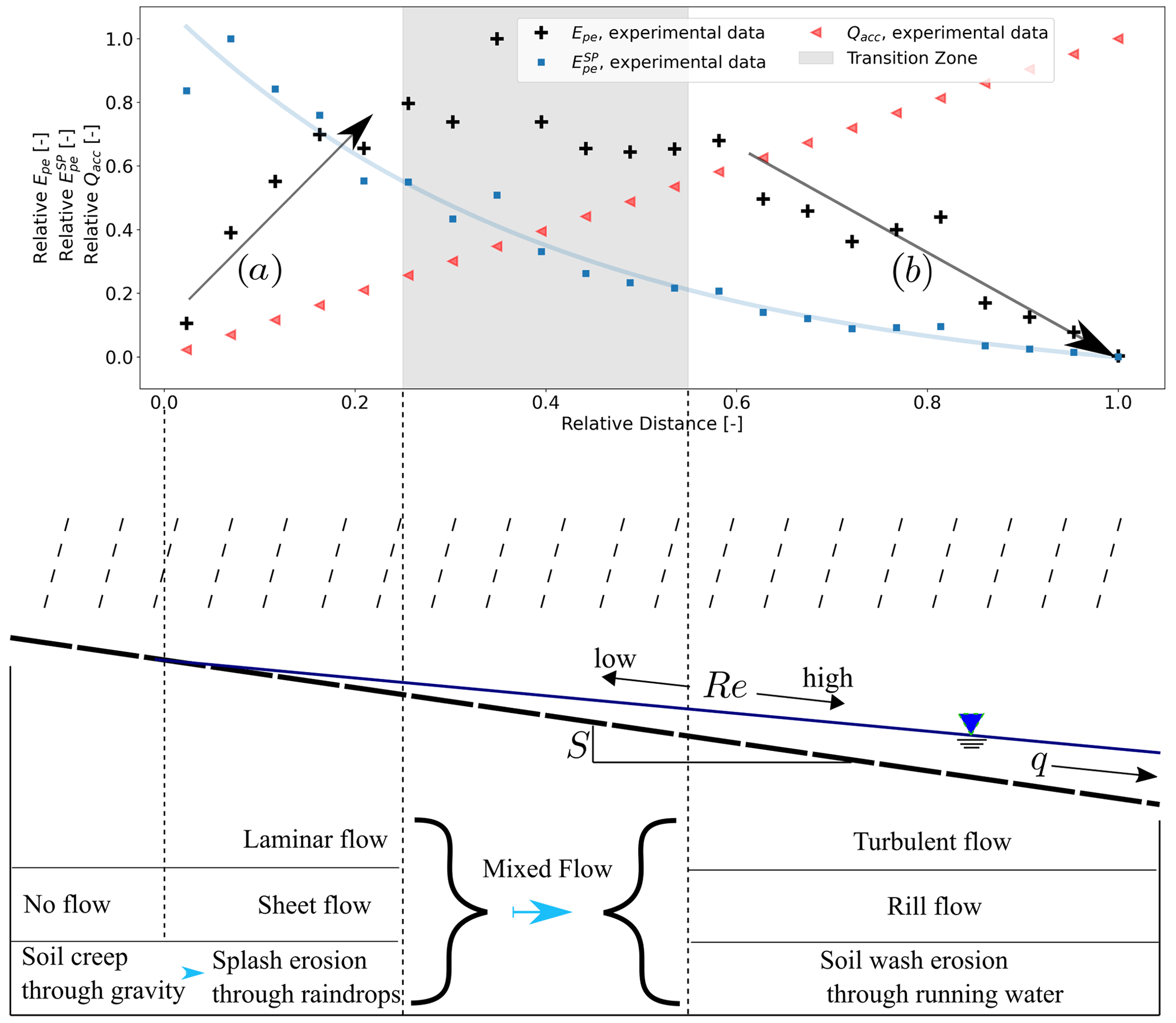
Figure 2Upper part: digitized results from rainfall simulation experiments at New Fork River 1 (Emmett, 1970), expressed as normalized potential energy , specific potential energy and Reynolds number Re. Lower part: simplification of overland flow processes on hillslopes (modified after Shih and Yang, 2009) as a function of Reynolds number Re and distribution of potential energy.
Rill structures form on event to seasonal timescales due to a fast positive feedback (Rieke-Zapp and Nearing, 2005). On a longer timescale, the redistribution and export of soil material restructures entire topographic hillslope profiles such that typical shapes can be attributed to a dominant erosion process (Kirkby, 1971; Beven, 1996). The latter change in space along the flow path and therefore in close connection to the flow regimes (Shih and Yang, 2009; see Fig. 2). At the upslope divide, erosion is mostly influenced by gravity, resulting in soil creep. With flow accumulation in a downslope direction, the particles eroded by raindrop splash can be transported by surface runoff, until surface runoff becomes turbulent and can erode and transport particles as soil wash. The spatial organization of transition processes (also called threshold processes) can be described by the relative contribution of internal and external forces. Turbulence emerges when gravitational (external) force surpasses a certain threshold in relation to viscous (internal) forces. Similarly, soil wash erosion relates to externally induced bed stress by runoff, while soil creep depends on internal resistance factors of the soil matrix. We therefore propose, as stated in our second hypothesis, that both process transitions are linked through their external forcing, which is attributed to the energy gradient of surface runoff. The distribution of surface runoff energy and its gradient provide therefore insights on erosional as well as flow regimes.
In the following we apply our framework to test our hypotheses on two related temporal and spatial scales. In Sect. 3, we analyse the distribution of energy at the macroscale, representing the hillslope as an open thermodynamic system which adapts morphologically to the distribution of gradients and fluxes on long timescales. To this end we analyse steady-state runoff on typical hillslope profiles that reflect, according to Kirkby (1971), the dominant erosion processes “soil creep”, “rainsplash” and “soil wash”. In Sect. 4 we analyse the energy balance of surface runoff observed during short-term rainfall simulation experiments, where runoff concentrates in rills and distributes energy into a sheet and a rill domain.
In both sections we explore how the transition of flow regime and erosion processes on hillslopes relate to the distribution of energy and its local maximum. We want to stress that we speak of laminar flow if there is a clear dependence between flow Reynolds number of surface runoff and friction coefficient (Phelps, 1975). For purpose of comparison with earlier studies of hydraulics of surface runoff (Emmett, 1970; Parsons et al., 1990) we calculate flow Reynolds number Re as per Eq. (10), relating the characteristic length of surface runoff to flow in a fully filled circular pipe. Here, v represents the depth averaged flow velocity, R is the hydraulic radius and ν is the kinematic viscosity with a value of 10−6 m2 s−1.
To clarify and test our hypothesis, we digitized results of rainfall runoff experiments on hillslope plots from Emmett (1970) and plotted potential energy and specific potential energy ( (Fig. 2, upper part) in parallel to a sketch of surface runoff on a hillslope and the related flow and erosion process transitions (Fig. 2, lower part). and were calculated from measured water depth above outlet reference level and mean flow velocity.
The accumulation of mass along a declining geopotential leads to a maximum of potential energy in space, dividing the flow path into a section where energy is gained (Fig. 2, arrow a) and a section where energy is depleted (Fig. 2, arrow b). In between these two sections (Fig. 2, area highlighted in grey), depletion of potential energy is balanced by the energy influxes of runoff accumulation and rainfall. Volumetric energy as well as its gradient decreases along the flow path. Or differently stated, the energy expenditure per unit discharge decreases in a downstream direction (solid blue line). This is very much in line with the previously mentioned principles of Rodriguez-Iturbe et al. (1992) and Yang (1976) of minimum stream power in river streams. To the best of our knowledge, a separation of the runoff system into an energy production and energy depletion zone has not been investigated so far but could have consequences on our understanding of the transitional formation of runoff and erosion processes on hillslopes.
The transition from a laminar into a turbulent-flow regime is indicated by ranges of critical Reynolds-number Rec, which depend on the type of flow as well as relative friction. While the Rec of circular pipe flow is roughly 2300 (Schlichting and Gersten, 2017), in field and laboratory experiments Emmett (1970) determined Rec of sheet flow between 1500 and 6000. Later Phelps (1975) pointed out that for sheet flow over rough surfaces Rec depends on relative friction k, which is the size of an average sediment particle to the depth of the flow. He showed that for k values of 0.5, Rec can be as low as 400. For the results presented in Fig. 2, Re was calculated with average depths and mean velocities along the slope direction and increased linearly up to 1368 at the lower end of the experimental plot. As however an analysis of the flow patterns suggests, local Re at points where flow converges into rills is likely to be much larger. A transition from a laminar- to a turbulent-flow regime in rills is therefore likely to correspond in Fig. 2 to a flow path distance within the highlighted transition zone between an increase and decrease in potential energy (mixed flow).
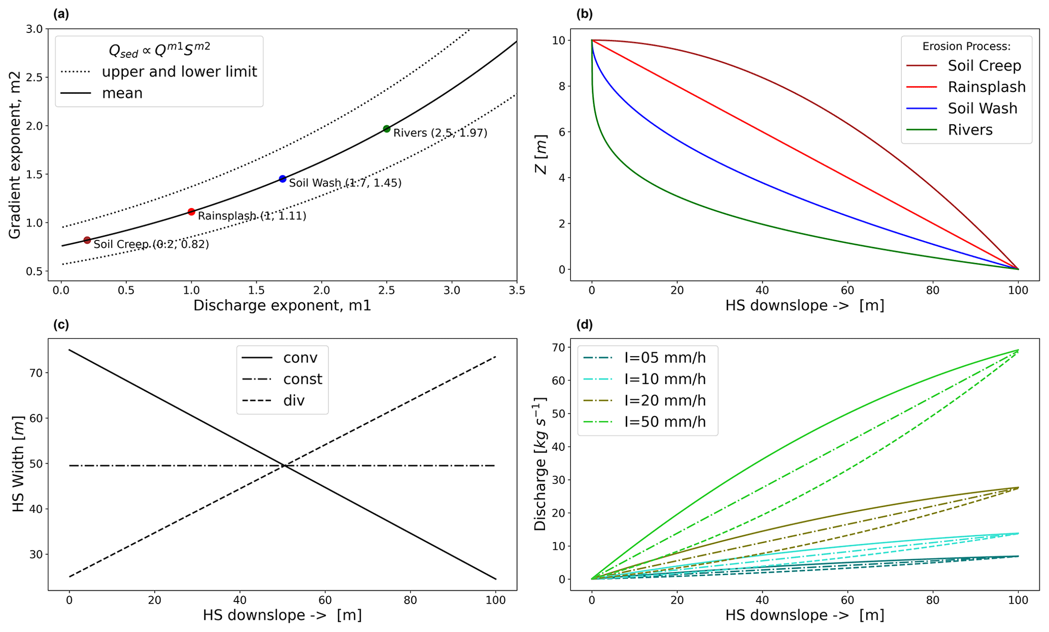
Figure 3(a) Discharge (m1) and gradient (m2) exponent (after Kirkby, 1990, cited in Beven, 1996) for characterizing sediment transport capacity, (b) typical hillslope (and river) profiles as a result of a dominant erosion process (Kirkby, 1971), (c) assumed width distributions along the flow path and (d) resulting steady-state discharge along the hillslope for different rainfall infiltration excess intensities. The line types in panel (d) correspond to the width functions in panel (c).
3.1 Typical hillslope forms and width functions
In this section, we explore how typical hillslope configurations and effective rainfall forcing control runoff accumulation and related energy conversions. We distinguish three typical hillslope forms, which are related to a dominant erosion process (Kirkby, 1971). Equation (11) defines the distribution of geopotential along a representative flow path. The coefficients m1 and m2 describe the relative contributions of accumulated discharge and topographic slope to sediment transport (). According to Kirkby (1971), the region m1<1 is therefore related to a hillslope profile that was formed by diffusive erosion processes (soil creep or rainsplash), whereas the region m1>1 corresponds to more advective erosion processes with higher sediment transport capacities (soil wash, river flow). We can therefore use these empirical coefficients to describe the transition of one regime (diffusive erosion/transport) into another (advective erosion/transport), if appropriate boundary conditions (rainfall and infiltration rates, vegetation, etc.) allow for long enough feedback to reach steady state.
A rough relation between coefficients m1 and m2 and corresponding erosion regions is shown in Fig. 3a (after Kirkby, 1990; cited in Beven, 1996). For selection of the coefficients that we use to relate hillslope form and sediment erosion/ transport regime, we digitized the upper and lower limits and computed a mean curve from which we extracted the coefficients m1 and m2 in accordance with ranges indicated by Kirkby (1971). In our example, all hillslopes start at Zmax=10 m, the maximum geopotential in metres above the stream bank, and end at zero at the hillslope end (XHS=100 m; see Fig. 3b), depleting all available geopotential gradients on the hillslope. We then combine these forms with three different width distributions, which are either constant (const), converging (conv) or diverging (div) (Fig. 3c). In our analysis we keep the projected area constant at 5000 m2 for all configurations, which results in an equal total surface runoff from all hillslope forms for a given effective rainfall intensity. Finally, we computed steady-state surface runoff for effective rainfall intensities of 5, 10, 20 and 50 mm h−1 (Fig. 3d). The differently dotted lines in Fig. 3c and d represent the three hillslope width distributions and show their influence on runoff accumulation. For all combinations of runoff accumulation and hillslope topography, we computed the steady-state spatial distribution of water mass and flow velocity using Eq. (6). From the computed hydraulic variables, we then calculated the distribution of potential energy flux and kinetic energy flux (see Appendix A).
3.2 Spatial maxima of potential energy
Generally, we found that the trade-off of downslope mass accumulation and declining geopotential leads to a distinct potential energy maximum, which has a clear dependence on the slope form, width function and strength of rainfall forcing (Fig. 4). This implies that the hillslope can be subdivided into three classes of spatial energy dynamics:
-
,
-
,
-
.
Within the first interval, potential energy flux increases along the flow path, as the additional mass from rainfall adds more energy to the sub-OTS than flows out. At a certain distance (interval 2), energy outflux equals energy influx through precipitation plus upstream inflow, and we observe an energetic maximum. Within the third interval, energy outflux is continuously larger than energy influx, effectively depleting the accumulated geopotential of interval 1.
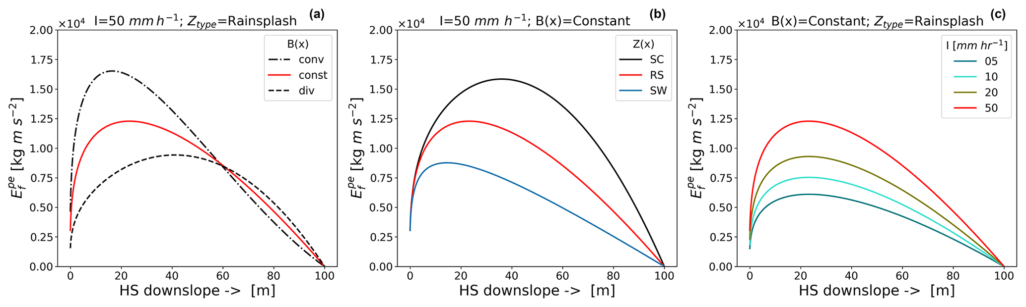
Figure 4Distribution of potential energy per unit length (J m−1) as a function of (a) hillslope width, (b) geopotential distribution (form) and (c) rainfall intensity I.
Figure 4a shows that the location of the energetic maximum moves upslope when changing the width function from divergent (div) to parallel (const) to convergent (conv). The magnitude of the absolute value of the maximum increases in a similar fashion. The distribution of geopotential from top to bottom clearly influences the location and size of maxima (Fig. 4b). Hillslope profiles which are formed by soil creep (SC) show the maximum of farthest downslope, whereas profiles related to rainsplash (RS) and soil wash (SW) erosion reach the maximum potential energy farther upslope. As potential energy has dissipated at the end of the hillslope, this implies that SC profiles dissipate more energy on shorter flow path distance than RS or SW profiles (indicated by the gradient of in Fig. 4b). If dissipation is proportional to bed stress (see discussion in Sect. 2.3), this means that for the same amount of energy input across the hillslope, larger bed stresses occur on SC profiles, while in comparison SW profiles relate to lower relative bed stress.
Similarly, an increasing rainfall infiltration excess intensity I increases the magnitude of the energy maxima, while it does not affect their location (Fig. 4c). Increasing energy maxima imply steeper energy gradients, resulting in more power during the energy conversion processes. We thus state that the distribution of potential energy in space is a function of hillslope width, form and rainfall intensity, and this seems to go hand in hand with the morphological stages of hillslope forms.
3.3 Topographic control of energy conversion rates
To estimate the relative amount of influx energy that is converted into the energy balance residual Df, for each hillslope form we compute the accumulated energy residual (watts) divided by accumulated steady-state energy input (watts) along the flow path:
If no other mass-affecting processes are considered, is the accumulated energy influx due to rainfall at flow path distance xl. Further we do not consider upslope runon at the hillslope top in steady state and , so that Eq. (12) becomes
At each point along the flow path, Eqs. (12) and (13) describe how much energy of the upslope-accumulated potential energy from rainfall is neither conserved as kinetic nor potential energy of the mean flow. The ratio is therefore a thermodynamic descriptor that can be used to estimate the dissipation per power, i.e. energy input, independent of absolute flow path lengths, rainfall rates and geopotential gradient. Similarly, the ratio describes the relative magnitude of upslope-accumulated input energy that is converted into kinetic energy at each cross section along the flow path.
Figure 5a reveals a distinct pattern of . For SW hillslope forms, the ratio is continuously larger than for RS and SC forms. Regardless of absolute energy influx, SW hillslope forms convert relatively more influx energy into Df than RS or SC forms. Similarly, but to a much smaller degree than profile form, hillslopes with converging widths dissipate relatively more energy on shorter flow path lengths compared to constant or diverging widths. For all forms, is almost completely dissipated at the end of the hillslope (), and only a minor part of is converted into kinetic energy (Fig. 5b and c: ). SW hillslope forms convert a larger part of the influx energy into kinetic energy than RS and SC forms, and the same hierarchy is found in converging to constant and to diverging hillslope widths (Fig. 5c). The function of kinetic energy along the flow path is convex, which relates to increasing production of kinetic energy per energy influx.
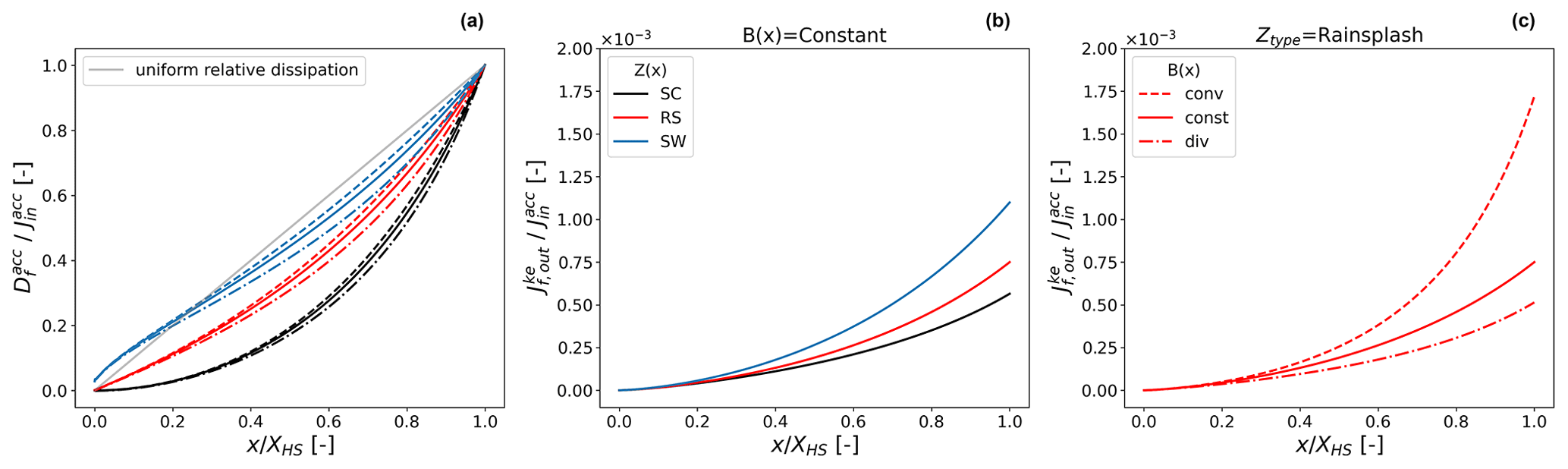
Figure 5Spatial distribution of the ratio of (a) accumulated dissipation and accumulated energy influx, (b) kinetic energy outflux and accumulated energy influx for constant hillslope width but varying hillslope forms and (c) kinetic energy outflux and accumulated energy influx for hillslope form related to rainsplash but varying hillslope width distributions.
3.4 Discussion
In this section we related the spatial distribution of slope (hillslope form) to the distribution of potential and kinetic energy of surface runoff. As form is also connected to the dominant erosion process, an analysis of energy dissipation provides a link between the erosion process and thermodynamic principles. In a first step we digitized surface runoff experiments by Emmett (1970), and we showed that the distribution of potential energy results in a distinct flow path distance with maximum potential energy. Up to this point, the system net accumulates energy and only undergoes a net loss of energy after this location. The distribution of these zones of energy production and energy depletion seems to be related to the transition of the system from one type of flow regime to another. Magnitude and distribution of energy are relative to a level of null energy at the hillslope end and therefore represent an assumed equilibrium state of the land–water system at the hillslope scale. From a larger perspective, the accumulated discharge at the end of the hillslope can perform work within the context of the whole catchment, which has been discussed previously (compare Rodriguez-Iturbe et al., 1992; Kleidon et al., 2013).
For an analysis of these equilibrium-state hillslopes, we relied on established semi-empirical descriptions of hillslope forms and related erosion processes (Kirkby, 1971), and we assumed that surface runoff on equilibrium hillslopes has dissipated all potential energy at the downslope end (usually the channel bank). The resulting steady-state distribution of potential energy of surface runoff was then calculated by a friction law that was established for stony hillslopes in Arizona (Nearing et al., 2017) but in essence expresses the tendency of a hillslope surface to spatially organize friction as a function of slope and has previously been established with different parameters for rill flow (Govers, 1992). We note that these studies were concerned with surfaces which had little to no vegetation influencing the resistance to erosion of the soil particles, meaning that morphological adaptations were predominantly due to surface runoff. In a similar fashion we did not account for vegetation and infiltration but should mention that these processes would certainly affect the steady-state energy balance and its residual presented here. Therefore, we stress that the presented distribution of potential energy is meant to approximate steady-state runoff on equilibrium hillslopes with respect to frictional adaptation without vegetation and situations with significant infiltration excess runoff.
The resulting distributions reveal that on hillslope forms which relate to diffusive erosion (SC slope forms), of surface runoff is found farther downslope but with relatively larger magnitude than for forms related to advective erosion (SW). The net energy depletion zone on SC slopes depletes therefore for the same runoff more energy on shorter flow path distance than SW or RS slope forms, which implies larger bed stress.
Energetically, this can be expressed as relative accumulated dissipation per energy influx . Interestingly we find that hillslope forms that relate to soil wash convert a larger part of the energy influx into Df than RS and SC related forms. This means that although absolute bed stress is larger for SC formations, SW forms maximize work per input energy and are therefore more dissipative in relative terms. This makes sense as Df incorporates energy needed for sediment detachment and transport and is in line with the theory that SW forms maximize kinetic energy per energy influx (Leopold and Langbein, 1962). From a thermodynamic perspective, this corresponds to an increase in entropy, as energy can be distributed across more energetic states if the ratio is larger. Similarly, the distribution of the derivative of is almost uniform for SW forms (compare grey, straight line in Fig. 5a), which relates to the equal energy expenditure hypothesis of optimal channel networks (Rodriguez-Iturbe et al., 1992) as well as to a constant production of entropy per unit discharge (Leopold and Langbein, 1962).
Our assessment is based on an empirical relation between flow velocity and unit discharge and therefore does not provide closure to the energy balance. However, Eq. (6) implicitly incorporates a spatial organization of relative friction (compare Sect. 2.2), which in accordance with our results seems to be supported by thermodynamic theory. Reversely, we show that maximum power and equal energy expenditure per unit discharge for surface runoff on hillslopes should result in friction laws like the ones proposed by Govers (1992) and Nearing et al. (2017). In fact, the proposed slope–velocity equilibrium by Nearing et al. (2005) seems to be a natural outcome of the equal energy expenditure, maximum power and maximum entropy concepts.
Finally, we want to point out that along a similar line of thought, Hooshyar et al. (2020) have recently shown that logarithmic mean elevation profiles of landscapes resemble the logarithmic mean velocity profile in wall-bounded turbulence. The authors concluded that these logarithmic profiles are a consequence of dimensional length-scale independence and therefore apply to different dynamical systems, possibly also to a much smaller hillslope scale. As these profiles were observed at an intermediate region and therefore are spatially transient, we believe they might relate to the transition from energy production to energy depletion proposed here, inspired by the well-known energy cascade of turbulent kinetic energy (Tennekes and Lumley, 1972).
We now explore the spatial distribution of potential energy in sheet and rill overland flow, which was observed during rainfall–runoff experiments carried out in the Weiherbach catchment (Gerlinger, 1997). Therefore, we built an extension to the physical hydrological model Catflow, which allows for the accumulation of flow from sheet flow areas into rills (Catflow-Rill). As these experiments were performed on 12 m plots with a uniform slope, they correspond to the rain-splash-dominated hillslope type, as shown in Fig. 3b.
4.1 Study area and experimental database
The Weiherbach catchment is an intensively cultivated catchment which is almost completely covered with loess up to a depth of 15 m (Scherer et al., 2012). It is located in the Kraichgau region, northwest of Karlsruhe in Germany. Because of the hilly landscape, the intensive agricultural use and the highly erodible loess soils, erosion is a serious environmental problem in the Kraichgau region. The Weiherbach itself has a catchment area of 6.3 km2 and is around 4 km long. Elevation ranges from 142 to 243 m above sea level; the slopes are long and gentle in the west and short and steep in the eastern part of the catchment. The climate is semi-humid, with a mean annual temperature of 10 ∘C (Scherer, 2008). More than 90 % of the catchment area is arable land or pasture, 7 % is forested and 2.5 % is paved (farmyards and roads). Severe runoff and erosion events are typically caused by thunderstorms in late spring and summer, when Hortonian overland flow dominates event runoff generation (Zehe et al., 2001). A comprehensive hydro-meteorological dataset, as well as data on soil hydraulic properties, soil erosion, and tracer and sediment transport, is available for the Weiherbach (Scherer et al., 2012; Schierholz et al., 2000).
Here we analyse 31 rainfall simulation experiments (Gerlinger, 1997; compare data in the Supplement), which were performed to explore formation of overland flow and the erodibility of the loess soils (Scherer et al., 2012). The rainfall simulators were designed to ensure both realistic rainfall intensities and kinetic energies on plots of 2 m by 12 m size. Rainfall intensity of experiments ranged between 34.4 and 62.4 mm h−1. Runoff and sediment concentrations in overland flow samples were derived from samples taken during the experiments. We categorized an experiment as reaching steady-state discharge if during the last time quarter, the relative change of discharge between measurements stays below 10 % measurement error (Fig. 6a). Likewise, we proceeded to classify measured sediment concentrations (Fig. 6b). The final steady-state classification of each experiment per discharge and sediment concentration can be found in the Supplemental of this paper. All but five experiments were classified as reaching steady-state discharge (Fig. 6a), while only nine were classified as reaching steady-state sediment concentrations (Fig. 6b). This means that only experiments which reached steady-state runoff as well as sediment concentrations can be considered as being truly in an energetic steady state (7 out of 31; compare data in the Supplement). The different sites were characterized according to their antecedent soil moisture, soil texture and organic content in the upper 5–10 cm (Scherer et al., 2012). Additionally, surface roughness (Manning's n) was estimated from the falling limb of the observed hydrograph (Engman, 1986; Govers et al., 2000). Observed rill flow velocities vRF,obs were measured by upslope tracer injection and correspond to the time it took until the peak of tracer concentration reached the plot outlet, while reported sheet flow velocities vSF,obs have been back-calculated from measured runoff rates. Further details on the experimental setup are provided by Gerlinger (1997), Seibert et al. (2011) and Scherer et al. (2012). A first analysis of the data already reveals that experimental sites with a larger value of Manning's n correspond to a smaller ratio , suggesting that a larger roughness leads to stronger accumulation of runoff in rills. As will be shown, this in turn relates to the portioning of kinetic energy between the sheet and rill domain.
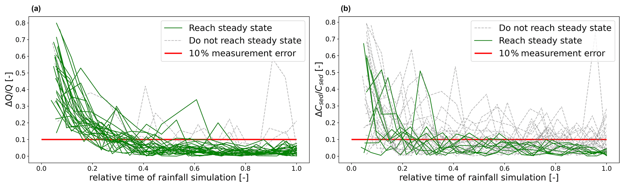
Figure 6Classification of rainfall simulation experiments, where green lines reach steady state during 0.75–1.0 of relative time of rainfall simulation: (a) relative change of discharge and (b) relative change of sediment concentration.
4.2 Model and model setup
Next, we present an extension to the Catflow model (Zehe et al., 2001), accounting for a dynamic link between sheet and rill flow of surface runoff. The model has previously been extended, incorporating water-driven erosion (Scherer, 2008), and has been shown to successfully portray the interplay of overland flow, preferential flow and soil moisture dynamics from the plot to small catchment scales (Graeff et al., 2009; Loritz et al., 2017; Zehe et al., 2005, 2013).
A catchment is represented in Catflow by a set of two-dimensional hillslopes (length and depth), which may be connected by a river network. Each hillslope is discretized using curvilinear orthogonal coordinates; the third dimension is represented by a variable width. Subsurface water dynamics are described by Richards' equation, which is solved numerically by an implicit mass-conservative Picard iteration scheme. The simulation time step for soil water dynamics is dynamically adjusted to achieve an optimal change of the simulated soil moisture, which assures fast convergence of the Picard iteration. Soil hydraulic properties are usually parameterized using the van Genuchten–Mualem model (Mualem, 1976; van Genuchten, 1980), but other options are available. Enhanced infiltrability due to activated macropore flow is conceptualized through enlarging the soil hydraulic conductivity by a macroporosity factor fmak when a soil moisture threshold is exceeded. This approach is motivated by the experimental findings of Zehe and Flühler (2001a, b) in the Weiherbach catchment and has been shown to be well suited for predicting rainfall–runoff dynamics (Zehe et al., 2005) as well as tracer transport at the plot and the hillslope scales (Zehe and Blöschl, 2004; Zehe et al., 2001).
4.2.1 Representation of overland flow in Catflow and Catflow–Rill
Overland flow is simulated in Catflow–Rill with the diffusion wave equation, which is numerically solved using an explicit upstreaming scheme, a simplification of the Saint-Venant equations for shallow water flow; for details of the numerical scheme we refer to Scherer (2008). Flow velocity is calculated with Manning's equation (Eq. 5). The previous Catflow model assumes sheet flow only. To incorporate a rill domain that dynamically interacts with sheet flow, we conceptualize the hillslope surface similar to the open-book catchment (Wooding, 1965) as an open-book hillslope (Fig. 7). In this configuration, water may accumulate in a trapezoidal rill of width Br in the middle of the open-book hillslope, with width BHS and downslope length LHS. Rainfall is added proportionally to the projected area along the flow path in both domains, resulting in spatially distributed sheet flow QSF and rill flow QRF. The link is established by a flow accumulation coefficient Cf (Eq. 14). This is visualized in Fig. 7 by the angle γ (in radians) between the vectors QSF and QRF, which, at each point on the sheet flow surface, manifest the tendency of a volume of water to flow downslope along the hillslope gradient α or to follow the secondary flow accumulation gradient β (Eq. 15).
The maximum amount of flow which is transferred per unit flow path length from the sheet domain into the rill domain is then given by
However, depending on the configuration of the open-book hillslope, we need to account for a flow path length LFC, where flow accumulation becomes constant and maximum:
From the hillslope top to the flow path length LFC, the flow accumulation coefficient is linearly interpolated between until .
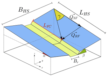
Figure 7Representation of overland flow domains in Catflow–Rill as an open-book hillslope: sheet flow domain (blue area) and rill flow domain (yellow area).
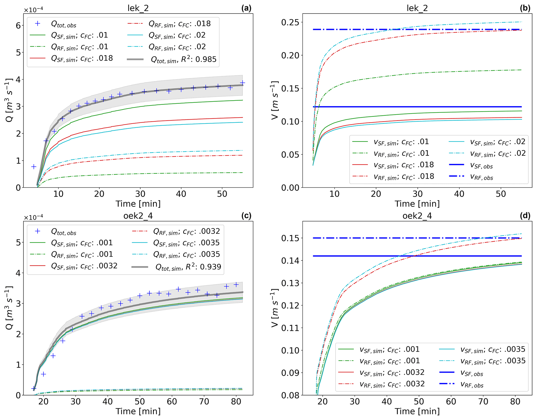
Figure 8Results of calibrations runs for experiments “lek_2” and “oek2_4”: (a, c) calibrated total discharge Qsim,tot, measured discharge Qtot,obs (inc. grey 10 % error band) and computed contributions of sheet flow QSF,sim and rill flow QRF,sim; (b, d) observed rill and sheet flow velocities vRF,obs and vSF,obs and calibration runs for different flow accumulation coefficients Cf.
4.2.2 Model setup and calibration of flow accumulation
From the experimental database, Scherer et al. (2012) created Catflow simulation setups, which were calibrated to reproduce runoff by adapting the macroporosity factor to scale infiltration capacity. The hillslopes were parameterized and initialized using observed data on average topographic gradient, plant cover, soil hydraulic functions, surface roughness, soil texture and antecedent soil moisture. The models were driven by a block rain of the respective intensity and duration of the experiment. From here onwards, the subscript “sim” relates to the results of the presented calibrated numerical simulations. Hillslopes were discretized on a 2D numerical grid with an average lateral distance of 60 cm and vertically increasing distances, starting with 1 cm at the surface and ending with 5 cm on the soil bottom. This resulted in 21×29 computational points for 12 m long, 2 m wide and 1 m deep hillslope plots. Soil hydraulic parameters of the Van Genuchten–Mualem model were reported by Schäfer (1999), who conducted a soil hydraulic parameter campaign within the Weiherbach catchment and classified five homogeneous soil types. From these, parameters from the Calcaric Regosol soil type were used for the presented simulations (Scherer, 2008) in accordance with the location of the experimental plots within the catchment (see Table 3). Grain size distributions are available with mean particle diameters d50 between 20 and 70 µm (Scherer, 2008; data in the Supplement).
Table 3Soil hydraulic parameters of Van Genuchten–Mualem model for simulated hillslopes, namely saturated hydraulic conductivity ks, saturated soil moisture θs, residual soil moisture θr, reciprocal air entry point αs, and soil hydraulic form parameters ns and γs.
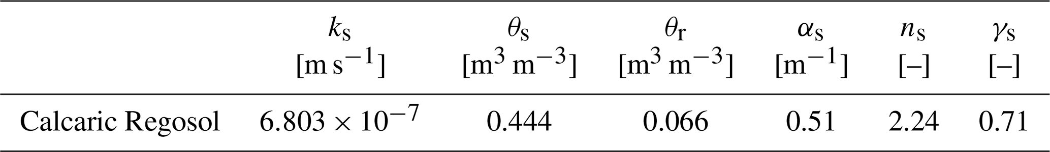

Figure 9Results of calibration of flow accumulation to observed rill flow velocities: (a) vRF,sim vs. vRF,obs, (b) vSF,sim vs. vSF,obs and (c) Cf vs. .
To match the observed flow velocities, we adjusted the flow accumulation coefficient Cf, starting at 0.001 and incrementing in 0.001 steps, compared the steady-state values of vRF,sim and vRF,obs, and stopped the incrementation of Cf when the residual of both values was below 1 % of vRF,obs (see Fig. 8b and d). Figure 8 shows the result of selected calibration iterations for the representative experiments “lek_2” and “oek2_4” to highlight the sensitivity to flow accumulation. For experiment lek_2 (slope = 0.163 m m−1), significant rill flow was reported (Gerlinger, 1997) with steady-state rill runoff velocities ( m s−1) almost double the average sheet flow velocities ( m s−1). Contrarily, during experiment oek2_4 (slope = 0.151 m m−1), little to no rill flow was observed, manifesting in almost equal surface runoff velocities of m s−1 and m s−1. For both hillslopes, the calibration produced good results after few incrementing steps. For lek_2 this resulted in Cf=0.018 and for oek2_4 in Cf=0.0032 (Fig. 8a and c). Total mass is conserved as total simulated discharge Qtot,sim () stays constant independent of Cf for all simulations, while discharge in the rill domain grows with Cf. Except for the onset of surface runoff, Qtot,sim stays with 10 % error tolerance bands of measured total discharge Qtot,obs for both experiments (compare Fig. 8a and c grey bands). While the observed rill flow velocities are matched well for both sites (lek_2 m s−1, oek2_4 m s−1), computed sheet flow velocities exhibit small deviations from the observed values. One reason might be the approach to calculate vSF indirectly from measured total discharge and vRF (Gerlinger, 1997) and the likely larger measurement errors. The final simulated steady-state value of vSF is however for both experiments within a 10 % error margin, which is tolerable in the light of measurement uncertainty.
4.3 Simulation results
4.3.1 Flow accumulation in rills
Figure 9 shows that calibrated rill flow velocities match the observed values for all 31 experiments well (Fig. 9a). We also note that magnitude of rill flow velocity is correlated to flow accumulation, ranging from the smallest, m s−1 and Cf=0.002, to the largest, m s−1 and Cf=0.024. In line with the observations, simulated rill flow velocities are not correlated to slope (Appendix B, Fig. B4). The resulting vSF,sim values are close to observed sheet velocities, with 23 out of 31 lying within 10 % measurement error (Fig. 9b, grey band). Outliers can partly be explained by classification of experiments reaching steady-state runoff QSS and/or steady-state sediment concentrations (compare Sect. 4.1 Fig. 6) and experiments which should not be considered steady state (QNSS and/or ; compare Fig. 9b). Simulations with the largest inconsistency between vSF,sim and vSF,obs are either classified as QNSS (Fig. 9b, marker “x”) or (Fig. 9b, coloured red) or both. In general, the proposed flow accumulation model slightly underestimates sheet flow velocities. Finally, we find a strong correlation between Cf and the ration of sheet to rill flow velocity (Fig. 9c), which can be represented as a power law (R2=0.82). In parallel we also find that Manning's n is positively correlated to Cf as well as vrat (compare Fig. 9c and Appendix B). The largest friction coefficients are therefore related to highest flow accumulation but lowest vrat values.
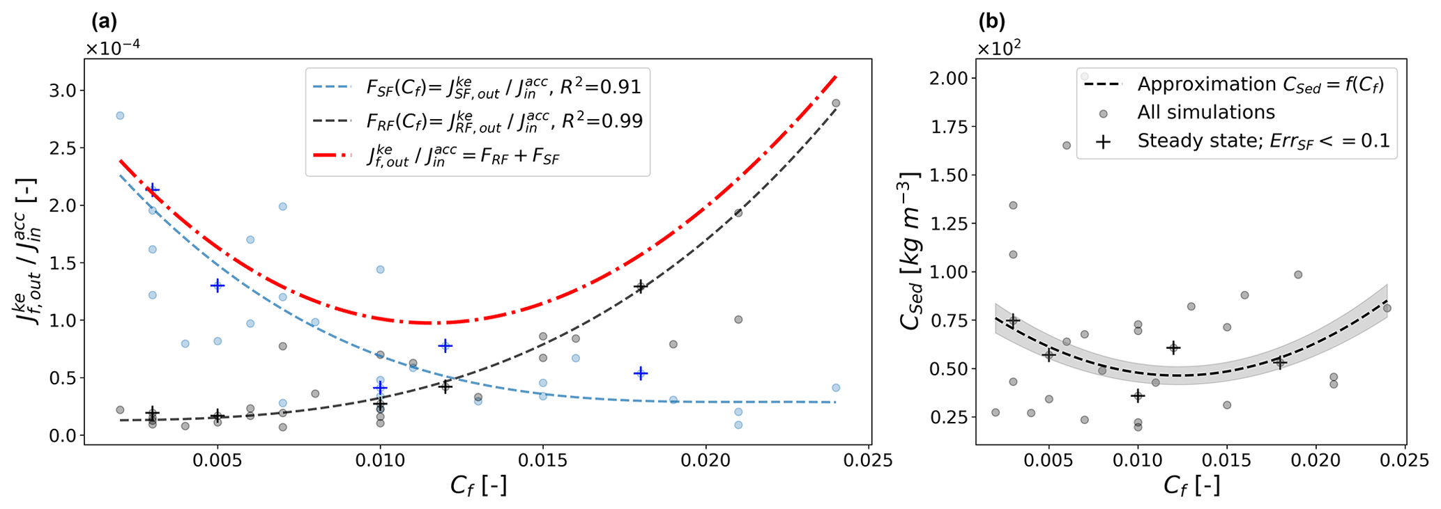
Figure 10(a) Relative flux of kinetic energy at the hillslope outlet as a function of flow accumulation for rill domain (FRF) and sheet domain (FSF) as well as total relative flux (FRF+FSF). (b) Measured sediment concentrations at hillslope outlet plotted against the flow accumulation parameter Cf; simulations with Err below 10 % and classified steady state are marked with “+”.

Figure 11Spatial distribution of (a) (maximum marked by black triangle) and (b) for calibrated rainfall runoff simulation lek_2, separated into sheet and rill flow.
4.3.2 Dissipation and erosion
In a similar fashion to the comparison of relative dissipation along the typical hillslope profiles in Sect. 3.3, we calculate the kinetic energy export at the hillslope end in relation to the potential energy influx by rainfall and compare the relative contributions of rill flow and sheet flow. However, we can only confidently evaluate this for simulated experiments which can be classified as steady state (for discharge and sediment concentrations; compare Fig. 6) and where vSF,sim matches vSF,obs sufficiently well (Fig. 9b). Considering all these requirements results in only 5 out of 31 simulations for which we can confidently compare relative dissipation rates to potential energy influx by rainfall as defined in Eq. (18). Consequently, as we analyse energy relative to hillslope outlet, potential energy is assumed to be completely dissipated or exported as kinetic energy at the hillslope end, so that Eq. (13) can be written as
implicitly incorporates rainfall intensity, slope and area of the hillslope and normalizes dissipation rates for comparison among the selected experiments. Figure 10a plots for the five trusted experiments (marked by “+”, high confidence) as well as for the 26 remaining simulations (marked by circle, low confidence). For each simulation we plotted the relative contribution of sheet flow FSF (blue) and rill flow FRF (black) against the flow accumulation coefficient, which sum up to total relative conversion rates of potential to kinetic energy. As the kinetic energy flux is proportional to Q3 (compare Eq. A4c, ), we analytically express FSF and FRF as cubic functions of accumulated discharge (), with Cf determining QRF and QSF. For each domain, Fig. 10a presents FRF and FSF of the fitted cubic function as well as their sum, which represents the total relative rate of kinetic energy export at the hillslope outlet as a function of flow accumulation in the rill domain. It is interesting to note that both functions also capture a significant portion of points which have been ruled out due to lower confidence and consequently were not included in the fit. As FSF declines and FRF increases with flow accumulation, total normalized kinetic energy export exhibits a distinct minimum value for Cf values in the range of 0.011 to 0.012 (Fig. 10a). This also corresponds to the region where relative kinetic energy export of rill flow and sheet flow are equal. According to Eq. (18), this equally means that the relative dissipation rate is maximized in this range of Cf values.
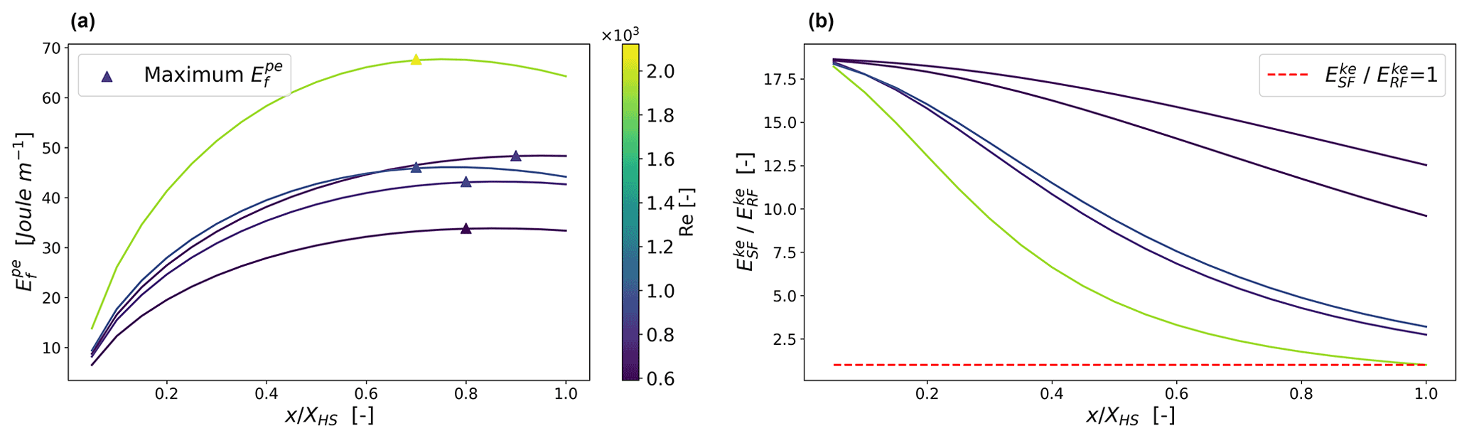
Figure 12Spatial distribution of (a) and (b) for considered experiments in the Weiherbach catchment (compare data in the Supplement); results are coloured by Re at hillslope distance of ).
4.3.3 Spatial distribution of energy and flow regimes
The calibrated Catflow–Rill models also provide an estimate of the spatial distribution of energy for the rill and the sheet domains. Figure 11a and b show the spatial distribution of potential energy (J m−1) and kinetic energy in each domain for an experiment with significant rill flow (lek_2; compare Fig. 8). First, we note that both approaches of runoff calculation (Cf=0 and Cf=Ccalib) result in a local maximum of potential energy and that most energy is stored within the sheet flow domain. The rill simulation increases potential energy within the rill domain and decreases in the sheet flow domain. This happens non-linearly, meaning relatively more energy is transferred from the sheet to the rill flow domain downslope than upslope. As a result, the location of maximum potential energy is shifted in an upslope direction and decreases in magnitude. The accumulation of runoff in rills leads to an increase in in the rill domain and contrarily a decrease in in the sheet domain in flow direction (Fig. 11b). For the calibrated experiment lek_2, kinetic energies of the two domains approach each other in a downslope direction and are almost equal at the hillslope end. As potential energy is up to 1000 times larger in magnitude than kinetic energy, the sum of free energies is essentially equivalent to . We further find that the accumulation of flow in a rill reduces the total amount of energy being stored on the hillslope.
By comparing five experiments classified as steady state (compare Fig. 10), we find that is shifted farther upslope for simulations with (a) higher maximum potential energy and (b) more runoff in rills (Fig. 12a). The latter becomes evident by estimation of Reynolds numbers of rill flow at the flow path length of maximum potential energy. The largest Re values are found for energy distributions with the maximum occurring farther upslope, and the smallest Re values are related to energy maxima appearing farther downslope. Computed Reynolds numbers at these maximum points range from 600 to 2100, which implies that the transition to a turbulent or at least a mixed-flow regime is possible.
Interestingly, the ratios of kinetic energy in a sheet to rill domain decline downslope, and the gradient of the curve increases (Fig. 12b) when the location and magnitude of is moving upslope. We observed that for one out of five experiments, the ratio reached unity (), while for the others, kinetic energy export in the sheet domain is dominant. We can therefore conclude that from the presented simulations, only experiments with significant rill flow approached unity within the 12 m plot lengths, while the plot length is too small for a final conclusion on experiments with less flow accumulation.
4.4 Discussion
Our approach to model the accumulation of surface runoff by a single rill and the calibration of a flow accumulation parameter resulted in partly good approximations of observed rill and sheet flow velocities and therefore justifies the presented simplification of surface runoff across two domains. Although the model uses a single friction coefficient (Manning's n), which is a simplification (compare Sect. 2.2), flow accumulation in a rill and the opposite flow dispersion of sheet flow led to spatially varying hydraulic radii, which imply variable friction along the hillslope. Manning's n, which was determined for each experiment (Gerlinger, 1997), is therefore closely related to flow accumulation and the ratio of sheet vs. rill flow velocity. Our results show that a larger friction coefficient leads to relatively more flow accumulation in rills, a phenomenon which was also observed in field experiments by Abrahams et al. (1990). Some of the simulations performed poorly on estimating sheet flow velocity (compare Fig. 9b and c); this can partly be explained by classification of experiments reaching steady-state discharge and sediment concentrations during the interval of rainfall simulation. Other outliers could be related to tilling, which is common on the hillslopes in the Weiherbach catchment. We conclude that for such conditions, experiments would have to be conducted for much longer durations, allowing for imprinted topographical structures of farming practices to be reversed and natural rill networks to emerge. Rieke-Zapp and Nearing (2005) applied rainfall with a maximum duration of 90 min to laboratory plots of 4 m by 4 m, and results suggested that rills had not reached an equilibrium steady state. Although the field plots have certainly been impacted by previous rain events and are therefore closer to an equilibrium state than a plane of laboratory sand, in retrospect it is not possible to judge the degree of perturbation due to farming. Nevertheless, the experiments clearly indicate that sheet and rill flow velocity are not a function of slope but depend on flow accumulation. The lowest flow velocities were observed for simulations with the lowest Cf coefficient and correlate up to the largest observed flow velocity and largest calibrated Cf (Fig. 9a; data in the Supplement). This is in line with the postulated slope–velocity theory on hillslopes (Govers et al., 2000; Nearing et al., 2005) and, according to our belief, is the result of a feedback between the friction coefficient and flow accumulation from sheet flow to flow in threads and then in rills.
Analysis of relative dissipation of energy per influx energy by rainfall reveals that surface runoff across the rill and sheet domain is related to the existence of a maximum power state. For the analysed experiments, we distinguished those which reached steady-state discharge and sediment concentrations and calculated the kinetic energy per influx energy that leaves the plot. For rill flow, it can be shown that kinetic energy export increases with flow accumulation, while kinetic energy of sheet flow decreases with growing Cf. As expected, kinetic energy flux of both domains can be approximated by cubic functions of Cf. The sum of both represents the total outflux of kinetic energy per potential energy input, which is characterized by a distinct range of flow accumulation that minimizes normalized kinetic energy export. Within this range, kinetic energy of both domains is approximately equal, and dissipation, expressed as the energy balance residual, is maximum (compare Fig. 10a). This finding is very similar to theoretical elaborations by Kleidon et al. (2013) on surface runoff and sediment export at the catchment scale, with an accumulation of channel flow from overland flow areas in a certain number of channels. As the number of channels grows, the distance of overland flow into the channel decreases, resulting in an optimal channel number with minimum dissipation. The difference between our argumentation and Kleidon's argumentation is that tectonic uplift and the depletion of slope gradient is negligible on the small hillslope plots in the Weiherbach catchment. In contrast to the study by Kleidon et al. (2013), sediment export should therefore not be maximized but minimized, with metastable hillslopes being related to hillslopes with minimum to no erosion. An assessment of observed sediment concentrations on the experimental plots indeed seems to indicate that minimum Csed might be related to minimum total kinetic energy per influx energy and therefore maximum relative dissipation (compare Fig. 10b). In this sense, the formation of rills is thermodynamically an expression of maximization of dissipation per influx energy from rainfall.
For the analysis of flow regime transitions (compare hypothesis 2), we plotted the Reynolds number of rill flow at the flow path distance where potential energy is maximum (compare Fig. 12a). While some Re values exceed the critical threshold for turbulence, others are below the value proposed by Emmett (). Yet, these low Re numbers might still relate to the onset of turbulent-flow regime as reported mean particle diameters are very small ( µm; compare data in the Supplement), resulting for very shallow runoff depths in high relative roughness and consequently a turbulent-flow regime at lower Re. Although spatially distributed mean water depths were not part of the experimental dataset, the results of the calibrated simulations clearly indicate that the distribution of potential energy relates to the transition from a laminar- to a turbulent-flow regime in a downslope direction.
Potential energy in this section is based on a relative calculation of potential energy with the null level of the 12 m plots at the outlet of the Weiherbach catchment, which makes the results (Fig. 12) comparable. We argue that surface runoff on hillslopes in its simplest case can be separated into sheet and rill flow and that the distribution of flow within both domains approaches a maximum power state over time (compare Fig. 10a). At this state dissipation per driving gradient is maximized, while the ratio of kinetic energies approach unity. We found that two of the truly steady-state sites as well as seven other experimental sites cluster in this area. In fact, we see very strong similarities to a maximum power state of an electrical circuit where the load resistance (in the case of surface runoff: the inverse of rill conveyance) has adjusted to meet the source resistance (the inverse of sheet flow conveyance; compare Appendix C). This finding can also be corroborated from Fig. 10a, with the minimum total flux of kinetic energy being related to equal fluxes of kinetic energy (and therefore also equal kinetic energies) across both surface runoff domains.
In this study we linked well-known processes of surface runoff (Shih and Yang, 2009) and erosion (Kirkby, 1971; Beven, 1996) to thermodynamic principles (Kleidon, 2016) and theories derived thereof (Leopold and Langbein, 1962; Rodriguez-Iturbe et al., 1992). The geomorphological development, surface runoff and the dominant erosion process co-evolve. We could show that an approach to account for the energy conversion and dissipation rates is a helpful unifying concept. The core of this concept is the residuals of the observable, free-energy fluxes and particularly their spatial distribution, which is key to evaluating empirical friction laws of surface runoff velocities in a thermodynamic framework. Although we do not provide a full closure of the energy balance of surface runoff, we were able to test and corroborate two hypotheses about the distribution of potential and kinetic energy of surface runoff and the related transition from laminar to turbulent flow, on two related hillslope scales. Hypothesis 1 states that surface runoff systems can be separated into an area of production and an area of depletion of energy. Our second hypothesis relates the typical transitioning of flow (laminar to turbulent) and erosion (diffusive to advective type) regime to these zones.
In line with our first hypothesis, we showed that hillslopes as mass-accumulating systems are characterized by a distinct energetic behaviour: the trade-off between downslope mass gain and geopotential loss along a runoff flow path leads to a maximum of potential energy. We found that the location and magnitude of this maximum are a function of hillslope form and accumulated surface runoff. Specifically, we analysed the influence of typical hillslope macro-topographical profiles with a fixed accumulated runoff on the spatial pattern of overland flow energy. We found that hillslope forms which relate to diffusive erosion processes (soil creep SC) have an energetic maximum located farther downslope than hillslope profiles related to advective erosion (soil wash SW). One might therefore be inclined to relate maximum dissipation rates to the former hillslope type SC as for our example more energy is depleted on a shorter flow path. However, in relative terms we see that SW forms have much larger dissipation rates than RS or SC forms, implying that dissipation is increased and even maximized as relative dissipation per unit flow path is close to unity. At the same time, SW forms also increase kinetic energy per influx energy, a criterion proposed by various authors for maximization of power (Kleidon et al., 2013) as well as maximum entropy production (Leopold and Langbein, 1962).
Referring to our second hypothesis, we interpret these findings as results of the transition of the dominant energy conversion process of surface runoff. Hereby we present a theory why laminar flow regime should be related to sheet flow and mixed/turbulent flow is related to concentrated flow in rills and channels. For the second application of this study, we create an extension to the numerical model Catflow, which allows for an adjustment of flow accumulation, by separating runoff into sheet and rill flow and dynamically linking both one dimensional flow domains. The calibration to observed rill and sheet flow velocities from rainfall simulation experiments in the Weiherbach catchments revealed distinct flow accumulation coefficients, which clearly relate to the distribution of kinetic energy of and the relative contribution to surface runoff from both domains. In fact, we showed that maximum relative dissipation rates are achieved when kinetic energy exports from both domains are equal. This can be interpreted as a maximum power state with minimum production of total kinetic energy, and related experiments therefore result in minimum sediment concentrations.
For those experiments that reached an energetic steady state, our simulations show that the build-up of potential energy on hillslopes is likely to occur under laminar flow conditions, while a decrease in potential energy along the flow path seems to be related to concentrated rill flow, with Re reaching values which classify as mixed- or turbulent-flow regime. We evaluated the Re at the flow path distance with maximum free energy in the simulated rill domain and found that values range between 600 and 2300, which is classified as the beginning of mixed and turbulent flow, depending on relative roughness. Although the rill model is a simplification of surface runoff, the well-matched rill and sheet flow velocities suggest that the model captures both runoff processes effectively. The results therefore present a valid estimate of the onset of mixed and turbulent flow by relating flow concentration to the distribution of energy production and depletion zones along the hillslope. The measurements at hand are certainly not comprehensive enough to allow for a final conclusion as to whether a maximum of free energy defines the onset of a turbulent-flow regime, but specifically designed and carefully measured experiments might reveal further insight on this. We would like to stress that the theory presented here applies to conditions where erosion is predominantly driven by surface runoff and not limited by vegetational and geological controls.
Our final comment is aimed at the common picture of runoff as a fixed volume of water losing energy by friction (e.g. Bagnold, 1966). We think that we have shown that this picture should be revised because a loss of mean flow energy does not necessarily imply an equal increase in production of heat but can also be translated into velocity fluctuations of turbulence or lift and accelerate sediment particles. All this affects real dissipation rates and needs to be considered if one ever attempts to depart from empirical friction laws of channel flow for estimation of surface runoff on hillslopes.
For each OTSsub we apply Eq. (4) where potential and kinetic energy of the system do not change with time, so that
For potential energy conversion, we obtain
while kinetic energy conversion is as follows:
To relate the spatial distribution of energy with energy fluxes, we recall that the downslope mass flux is associated with a downslope flux of kinetic and potential energy. The net fluxes correspond to the divergence of the kinetic and potential energy flow. in watts is defined here as the advective energy flux, which is the product of specific energy Esp, in joules per kilogram (J kg−1), and flow rate ρQ, in kilograms per second (kg s−1). As per the definition of Eq. (A4), Jf,net is positive for a decrease in energy flux over the control volume and therefore has the opposite sign to a change in energy:
Inserting the expressions for specific potential and kinetic energy (Eqs. A5 and A6) into Eqs. (A2) and (A3), we get power (Eq. A7) and dissipation (Eq. A8) of flow energy per unit length in watts per metre (W m−1):
Figures B1 to B4 are based on values derived from measurements (Manning's n, vRF, vSF, slope) and calibrated (Cf) values for all 31 analysed rainfall simulation experiments (see Gerlinger, 1997; data in the Supplement). Correlation was expressed by a power law which was fitted to mean bin values containing at least two values or more.

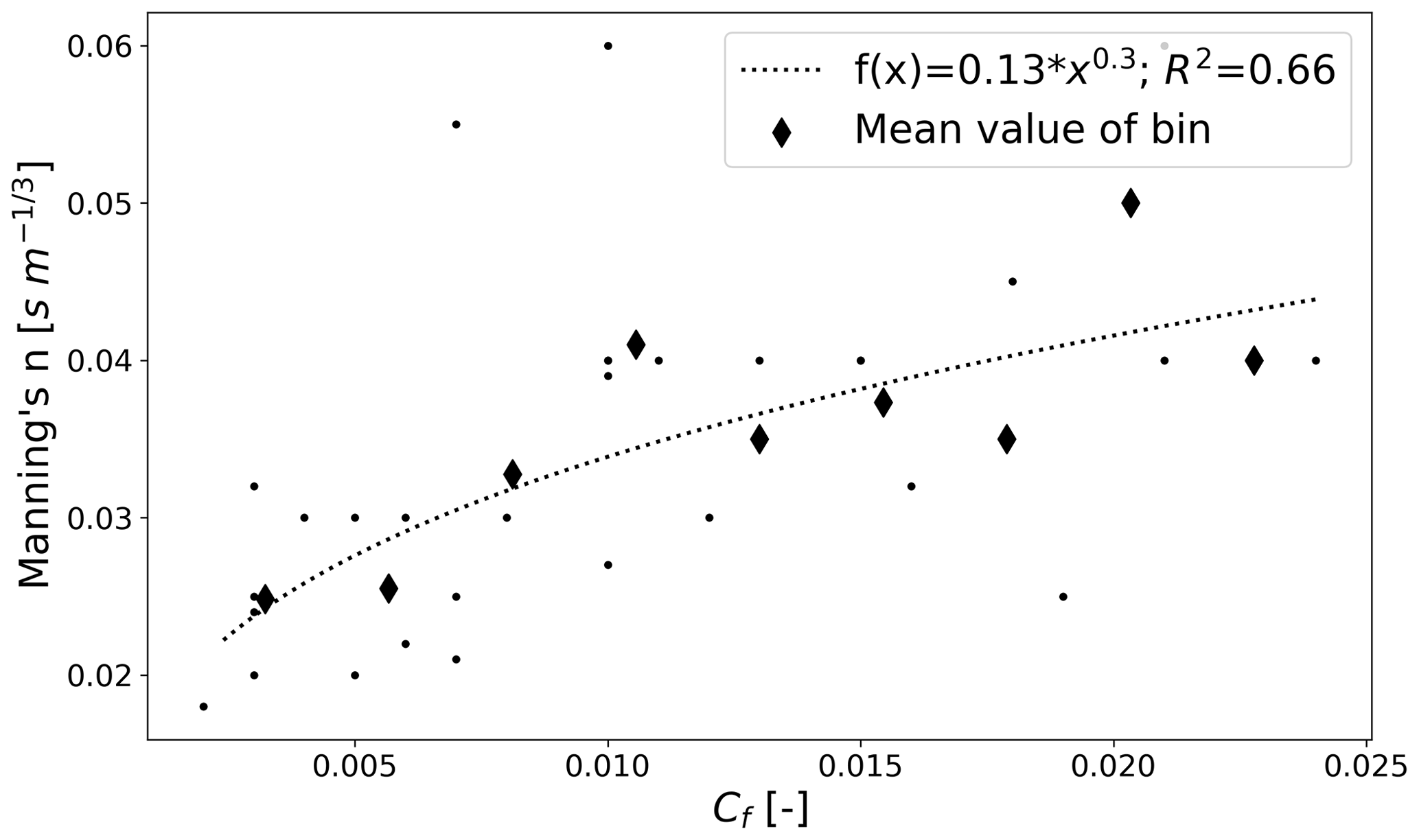
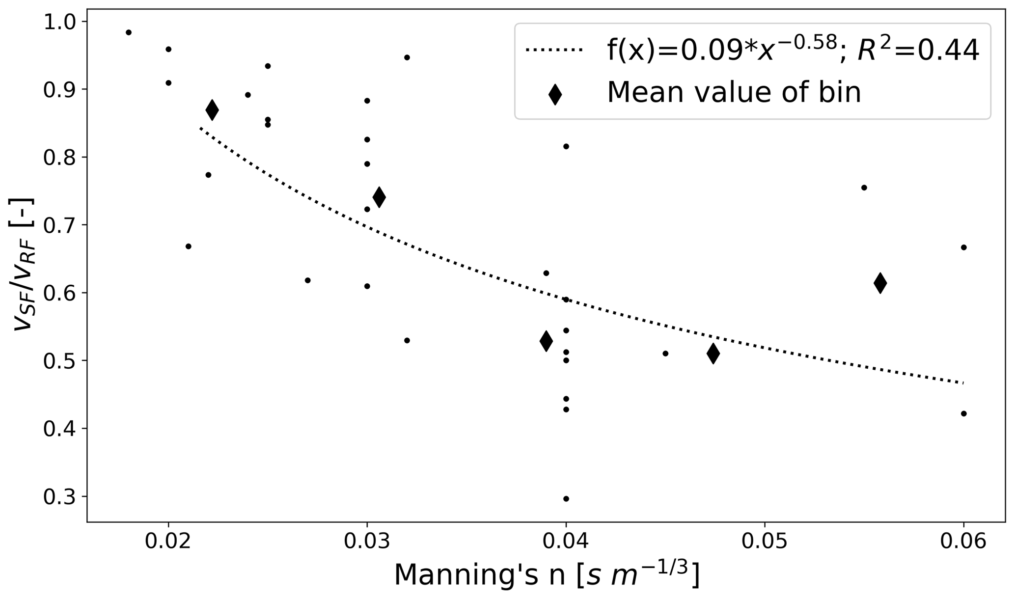
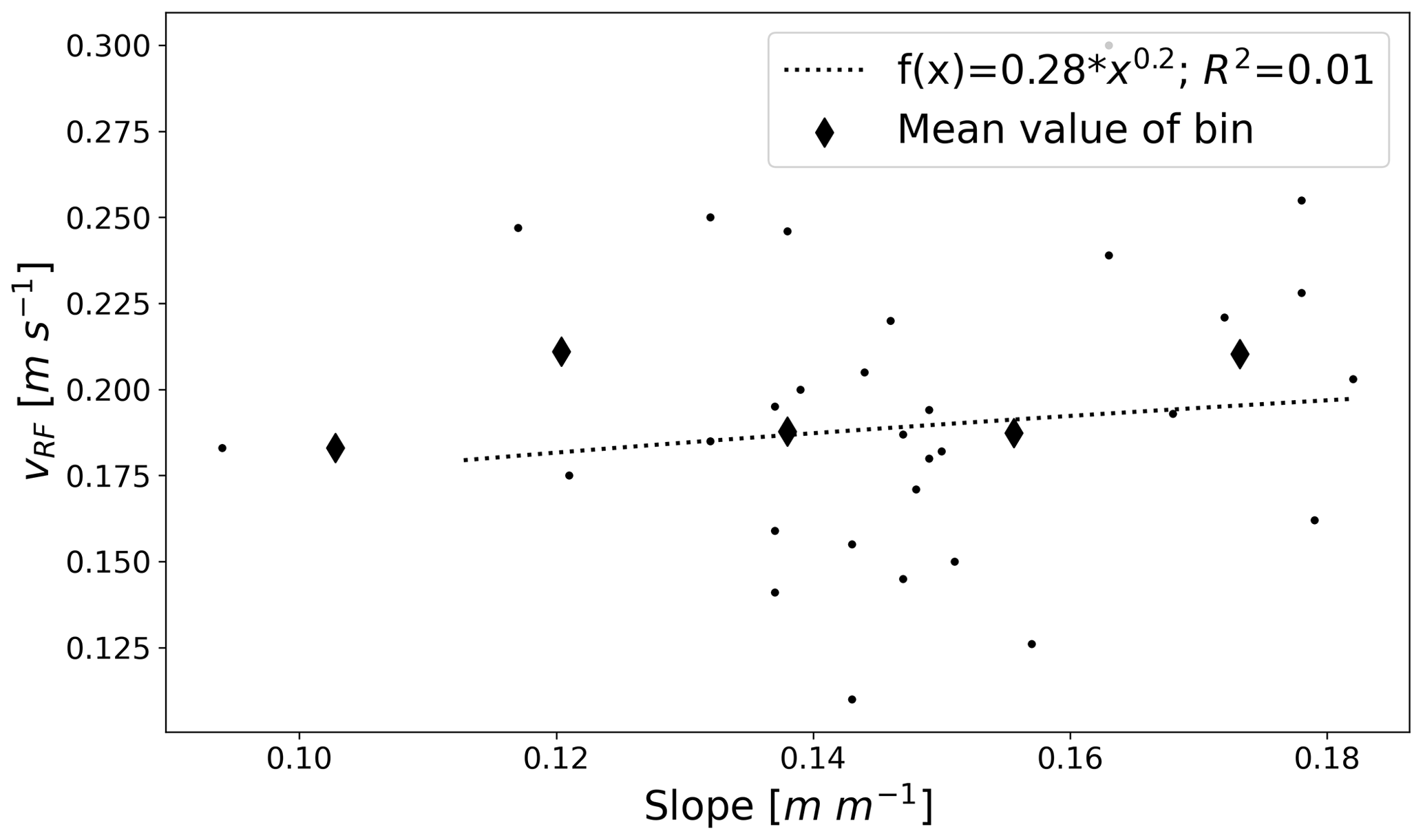
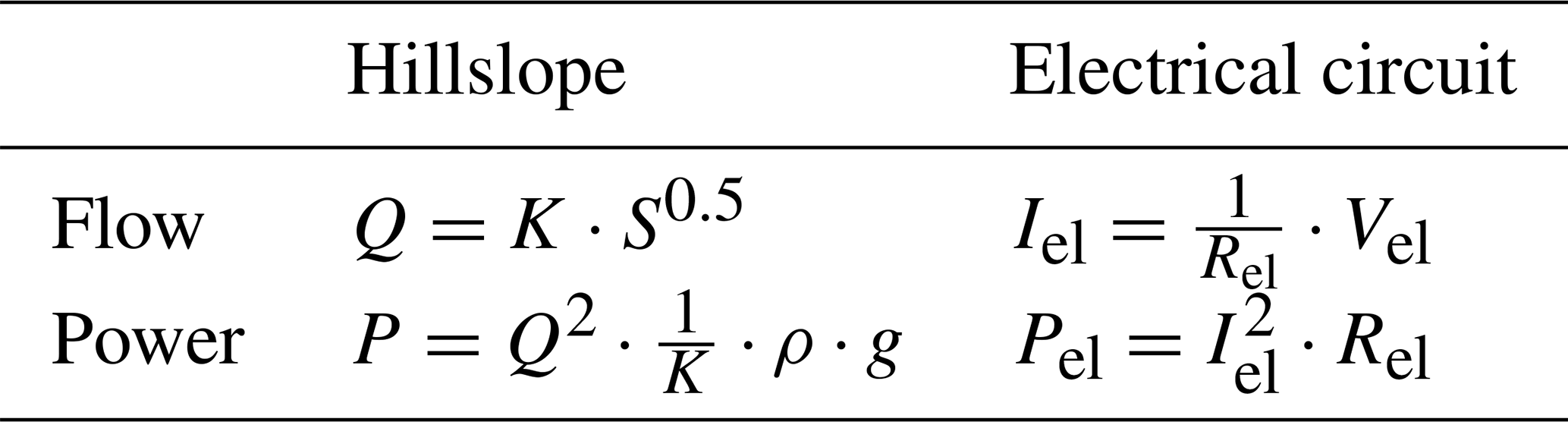
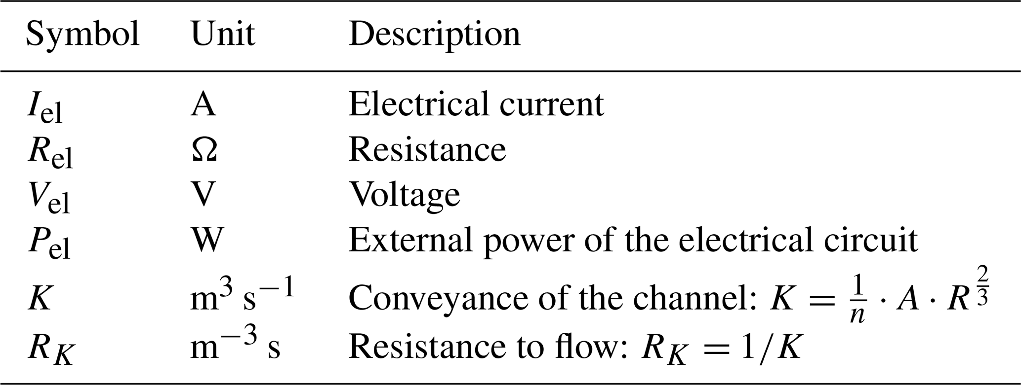
Therefore, channel conveyance is the inverse of the resistance of the channel to transport flow.
If water is mainly falling on the sheet flow area and flows therefore first onto the sheet flow area with and then accumulates in a channel with , the total resistance to flow is
Here we assume that is fixed and that mainly resistance to flow of the rill adapts.
Total power in the rill is then
Equation (C2) becomes maximum if the term “T” becomes minimum:
The derivative (Eq. C3) becomes zero if
or, equivalently,
The model code used is available upon request.
The used dataset (Gerlinger, 1997) has been published by the KIT and is accessible through its library. A summarized file is available on request.
The supplement related to this article is available online at: https://doi.org/10.5194/hess-26-3125-2022-supplement.
SSc conceptualized and implemented the Catflow–Rill extension, conducted the analysis and wrote the paper. OE conceptualized and supervised the hydraulic concepts. AK reviewed and edited the thermodynamic concepts. US provided the original Catflow setups and commented on surface runoff dynamics. JW contributed to paper writing and Catflow modelling. EZ oversaw the study and theory development as a mentor.
At least one of the (co-)authors is a member of the editorial board of Hydrology and Earth System Sciences. The peer-review process was guided by an independent editor, and the authors also have no other competing interests to declare.
Publisher's note: Copernicus Publications remains neutral with regard to jurisdictional claims in published maps and institutional affiliations.
We would like to thank the reviewers Keith Beven and Hubert Savenije for their valuable comments. Especially the discussion with Keith Beven was very appreciated and led to a substantial improvement of this paper.
The article processing charges for this open-access publication were covered by the Karlsruhe Institute of Technology (KIT).
This paper was edited by Roger Moussa and reviewed by Keith Beven, Hubert H. G. Savenije, and two anonymous referees.
Abrahams, A. D., Parsons, A. J., and Shiu-Hung, L.: Field experiments on the resistance to overland flow on desert hillslopes, in: Erosion, Transport and Deposition Processes, Proceedings of the Jerusalem Workshop, March–April 1987, Jerusalem, IAHS Publ. 189, 1990.
Abrahams, A. D., Parsons, J. D., and Wainwright, J.: Resistance to overland flow on semiarid grassland and shrubland hillslopes, Walnut Gulch, southern Arizona, J. Hydrol., 156, 431–446, 1994.
Achten, W. M. J., Dondeyne, S., Mugogo, S., Kafiriti, E., Poesen, J., Deckers, J., and Muys, B.: Gully erosion in South Eastern Tanzania: spatial distribution and topographic thresholds, Z. Geomorphol., 52, 225–235, https://doi.org/10.1127/0372-8854/2008/0052-0225, 2008.
Ali, M., Sterk, G., Seeger, M., Boersema, M., and Peters, P.: Effect of hydraulic parameters on sediment transport capacity in overland flow over erodible beds, Hydrol. Earth Syst. Sci., 16, 591–601, https://doi.org/10.5194/hess-16-591-2012, 2012.
Bagnold, R. A.: An approach to the sediment transport problem from general physics, US Geol. Surv. Prof. Paper 422-I, US Geological Survey, https://pubs.usgs.gov/pp/0422i/report.pdf (last access: 15 June 2022), 1966.
Bejan, A. and Lorente, S.: The constructal law of design and evolution in nature, Philos. T. Roy. Soc. Lond. B, 365, 1335–1347, https://doi.org/10.1098/rstb.2009.0302, 2010.
Berger, C., Schulze, M., Rieke-Zapp, D. H., and Schlunegger, F.: Rill development and soil erosion: a laboratory study of slope and rainfall intensity, Earth Surf. Proc. Land., 35, 1456–1467, 2010.
Berkowitz, B. and Zehe, E.: Surface water and groundwater: unifying conceptualization and quantification of the two “water worlds”, Hydrol. Earth Syst. Sci., 24, 1831–1858, https://doi.org/10.5194/hess-24-1831-2020, 2020.
Beven, K. J.: Equifinality and uncertainty in geomorphological modelling, in: The Scientific Nature of Geomorphology, edited by: Rhoads, B. L. and Thorn, C. E., Wiley, Chichester, 289–313, ISBN 0-471-96811-0, 1996.
Beven, K. J.: Robert E. Horton's perceptual model of infiltration processes, Hydrol. Process., 18, 3447–3460, https://doi.org/10.1002/hyp.5740, 2004.
Dunne, T. and Black, R. D.: An experimental investigation of runoff production in permeable soils, Water Resour. Res., 6, 478–490, https://doi.org/10.1029/WR006i002p00478, 1970.
Dunne, T. and Dietrich, W. E.: Experimental investigation of Horton overland flow on tropical hillslopes. Part II: Hydraulic characteristics and hillslope hydrographs, Z. Geomorphol., 35, 60–80, 1980.
Emmett, W. W.: The Hydraulics of Overland Flow on Hillslopes, US Geol. Surv. Prof. Paper 662, US Geological Survey, https://pubs.usgs.gov/pp/0662a/report.pdf (last access: 15 June 2022), 1970.
Engman, T. E.: Roughness coefficients for routing surface runoff, J. Irrig. Drain. Eng., 112, 39–53, 1986.
Evans, R. and Taylor, J.: Some methods of directly assessing water erosion of cultivated land – a comparison of measurements made on plots and in fields, Prog. Phys. Geogr., 19, 115–129, 1995.
Faulkner, H.: Connectivity as a crucial determinant of badland morphology and evolution, Geomorphology, 100, 91–103, https://doi.org/10.1016/j.geomorph.2007.04.039, 2008.
Gerlinger, K.: Erosionsprozesse auf Lössböden: Experimente und Modellierung, Dissertation, Nr. 194, Mitteilungen des Institutes für Wasserbau und Kulturtechnik der Universität Karlsruhe (TH), Karlsruhe, 1997.
Gómez, J. A., Darboux, F., and Nearing, M. A.: Development and evolution of rill networks under simulated rainfall, Water Resour. Res., 39, 1148, https://doi.org/10.1029/2002WR001437, 2003.
Govers, G.: Relationship between discharge, velocity and flow area for rills eroding loose, non-layered materials, Earth. Surf. Proc. Land., 17, 515–528, 1992.
Govers, G., Takken, I., and Helming, K.: Soil roughness and overland flow, Agronomie, 20, 131–146, https://doi.org/10.1016/0304-1131(75)90001-6, 2000.
Graeff, T., Zehe, E., Reusser, D., Lück, E., Schröder, B., Wenk, G., John, H., and Bronstert, A.: Process identification through rejection of model structures in a mid-mountainous rural catchment: observations of rainfall-runoff response, geophysical conditions and model inter-comparison, Hydrol. Process., 23, 702–718, https://doi.org/10.1002/hyp.7171, 2009.
Hooshyar, M., Bonetti, S., Singh, A.; Foufoula-Georgiou, E., and Porporato, A.: From turbulence to landscapes: Logarithmic mean profiles in bounded complex systems, Phys. Rev. E, 102, 33107, https://doi.org/10.1103/PhysRevE.102.033107, 2020.
Horton, R. E.: Erosional development of streams and their drainage basins; Hydrophysical approach to quantitive morphology, Bull. Geol. Soc. Am., 56, 275–370, 1945.
Howard, A. D.: Theoretical Model of Optimal Drainage Networks, Water Resour. Res., 9, 2107–2117, 1990.
Ijjasz Vasquez, E. J., Bras, R. L., Rodriguez-Iturbe, I., Rigon, R., and Rinaldo, A.: Are river basins optimal channel networks?, Adv. Water Resour., 16, 69–79, 1993.
Kirkby, M. J.: Hillslope process-response models based in the continuity equation, Spec. Publ. Inst. Brit. Geogr., 3, 15–30, 1971.
Kleidon, A.: Thermodynamic foundations of the Earth system, Cambridge University Press, New York, NY, ISBN 9781107029941, 2016.
Kleidon, A., Zehe, E., Ehret, U., and Scherer, U.: Thermodynamics, maximum power, and the dynamics of preferential river flow structures at the continental scale, Hydrol. Earth Syst. Sci., 17, 225–251, https://doi.org/10.5194/hess-17-225-2013, 2013.
Kleidon, A., Renner, M., and Porada, P.: Estimates of the climatological land surface energy and water balance derived from maximum convective power, Hydrol. Earth Syst. Sci., 18, 2201–2218, https://doi.org/10.5194/hess-18-2201-2014, 2014.
Lawrence, D. S. L.: Macroscale surface roughness and frictional resistance in overland flow, Earth. Surf. Proc. Land., 22, 365–382, 1997.
Leopold, L. B., Langbein, W. B., and Walter, B.: The concept of entropy in landscape evolution, US. Geol. Surv. Prof. Paper 500-A, US Geological Survey, https://doi.org/10.3133/pp500A, 1962.
Loritz, R., Hassler, S. K., Jackisch, C., Allroggen, N., van Schaik, L., Wienhöfer, J., and Zehe, E.: Picturing and modeling catchments by representative hillslopes, Hydrol. Earth Syst. Sci., 21, 1225–1249. https://doi.org/10.5194/hess-21-1225-2017, 2017.
Mualem, Y.: A new model for predicting the hydraulic conductivity of unsaturated porous media, Water Resour. Res., 12, 513–522, https://doi.org/10.1029/WR012i003p00513, 1976.
Nearing, M. A., Kimoto, A., Nichols, M. H., and Ritchie, J. C.: Spatial patterns of soil erosion and deposition in two small, semiarid watersheds, J. Geophys. Res., 110, F04020, https://doi.org/10.1029/2005JF000290, 2005.
Nearing, M. A., Polyakov, V. O., Nichols, M. H., Hernandez, M., Li, L., Zhao, Y., and Armendariz, G.: Slope–velocity equilibrium and evolution of surface roughness on a stony hillslope, Hydrol. Earth Syst. Sci., 21, 3221–3229, https://doi.org/10.5194/hess-21-3221-2017, 2017.
Paik, K. and Kumar, P.: Optimality approaches to describe characteristic fluvial patterns on landscapes, Philos. T. Roy. Soc. Lond. B, 365, 1387–1395, https://doi.org/10.1098/rstb.2009.0303, 2010.
Paltridge, G. W.: Climate and thermodynamic systems of maximum dissipation, Nature, 279, 630–631, https://doi.org/10.1038/279630a0, 1979.
Parsons, A. J., Abrahams, A. D., and Luk, S. H.: Hydraulics of interrill overland flow on a semi-arid hillslope, Arizona, J. Hydrol., 117, 255–273, 1990.
Phelps, H. O.: Friction coefficients for laminar sheet flow over rough surfaces, Proc. Inst. Civ. Eng., 59, 21–41, https://doi.org/10.1680/iicep.1975.3840, 1975.
Rieke-Zapp, D. H. and Nearing, M. A.: Slope shape effects on erosion: a laboratory study, Soil Sci. Soc. Am. J., 69, 1463–1471, 2005.
Rodriguez-Iturbe, I., Rinaldo, A., Rigon, R., Bras, R. L., Marani, A., and Ijjasz-Vasquez, E.: Energy dissipation, runoff production, and the threedimensional structure of river basins, Water Resour. Res., 4, 1095–1103, 1992.
Rodriguez-Iturbe, I., Marani, M., Rigon, R., and Rinaldo, A.: Self-organized river basin landscapes: Fractal and multifractal characteristics, Water Resour. Res., 30, 3531–3539, https://doi.org/10.1029/94WR01493, 1994.
Schäfer, D.: Bodenhydraulische Eigenschaften eines Kleineinzugsgebietes – Vergleich und Bewertung unterschiedlicher Verfahren, Dissertation, Dissertationsreihe am Institut für Hydromechanik, KIT – Karlsruher Institut für Technologie, Karlsruhe, 1999.
Scherer, U.: Prozessbasierte Modellierung der Bodenerosion in einer Lösslandschaft, Karlsruhe, Schriftenreihe SWW 129, Univ., Diss., https://publikationen.bibliothek.kit.edu/1000009238/433441 (last access: 15 June 2022), 2008.
Scherer, U., Zehe, E., Träbing, K., and Gerlinger, K.: Prediction of soil detachment in agricultural loess catchments: Model development and parameterisation, Catena, 90, 63–75, https://doi.org/10.1016/j.catena.2011.11.003, 2012.
Schierholz, I., Schäfer, D., and Kolle, O.: The Weiherbach data set: An experimental data set for pesticide model testing in the field scale, Agr. Water Manage., 44, 43–61, https://doi.org/10.1016/S0378-3774(99)00083-9, 2000.
Schlichting, H. and Gersten, K.: Boundary-Layer Theory, Springer, Berlin, Heidelberg, https://doi.org/10.1007/978-3-662-52919-5, 2017.
Schumm, S. A., Harvey, M. D., and Watson, C. C.: Incised Channels: Morphology, Dynamics and Control, Water Resources Publications, ISBN 978-1887201643, 1984.
Seibert, S., Auerswald, K., Fiener, P., Disse, M., Martin, W., Haider, A. M., and Gerlinger, K.: Surface runoff from arable land – a homogenized data base of 726 rainfall simulation experiments, CRC/TR32 Database (TR32DB), https://doi.org/10.1594/GFZ.TR32.2, 2011.
Shih, H. M. and Yang, C. T.: Estimating overland flow erosion capacity using unit stream power, Int. J. Sediment Res., 24, 46–62, https://doi.org/10.1016/S1001-6279(09)60015-9, 2009.
Singh, V. P.: On the Theories of Hydraulic Geometry, Int. J. Sediment Res., 18, 196–218, 2003.
Smart, J. S.: Channel networks, Adv. Hydrosci., 8, 305–346, 1972.
Tennekes, H. and Lumley, J. L.: A first course in turbulence, MIT Press, Cambridge, Mass., ISBN 978-0-262-20019-6, 1972.
van Genuchten, M. T.: A closed-form equation for predicting the hydraulic conductivity of unsaturated soils, Soil Sci. Soc. Am. J., 44, 892–898, https://doi.org/10.2136/sssaj1980.03615995004400050002x, 1980.
Wooding, R. A.: A hydraulic model for the catchment-stream problem, J. Hydrol., 3, 254–267, https://doi.org/10.1002/9781118925935.ch2, 1965.
Yang, C. T.: Potential Energy and Stream Morphology, Water Resour. Res., 7, 311–322, 1971.
Yang, C. T.: Minimum Unit Stream Power and Fluvial Hydraulics, J. Hydraul. Div., 102, 919–934, https://doi.org/10.1061/JYCEAJ.0004589, 1976.
Zehe, E. and Blöschl, G.: Predictability of hydrologic response at the plot and catchment scales: Role of initial conditions, Water Resour. Res., 40, W10202, https://doi.org/10.1029/2003WR002869, 2004.
Zehe, E. and Flühler, H.: Preferential transport of isoproturon at a plot scale and a field scale tile-drained site, J. Hydrol., 247, 100–115, https://doi.org/10.1016/S0022-1694(01)00370-5, 2001a.
Zehe, E. and Flühler, H.: Slope scale variation of flow patterns in soil profiles, J. Hydrol., 247, 116–132, https://doi.org/10.1016/S0022-1694(01)00371-7, 2001b.
Zehe, E. and Sivapalan, M.: Threshold behaviour in hydrological systems as (human) geo-ecosystems: manifestations, controls, implications, Hydrol. Earth Syst. Sci., 13, 1273–1297, https://doi.org/10.5194/hess-13-1273-2009, 2009.
Zehe, E., Maurer, T., Ihringer, J., and Plate, E.: Modeling water flow and mass transport in a loess catchment, Phys. Chem. Earth Pt. B, 26, 487–507, https://doi.org/10.1016/S1464-1909(01)00041-7, 2001.
Zehe, E., Becker, R., Bárdossy, A., and Plate, E.: Uncertainty of simulated catchment runoff response in the presence of threshold processes: Role of initial soil moisture and precipitation, J. Hydrol., 315, 183–202, https://doi.org/10.1016/j.jhydrol.2005.03.038, 2005.
Zehe, E., Blume, T., and Blöschl, G.: The principle of `maximum energy dissipation': a novel thermodynamic perspective on rapid water flow in connected soil structures, Philos. T.e Royal Soc. Lond. B, 365, 1377–1386, https://doi.org/10.1098/rstb.2009.0308, 2010.
Zehe, E., Ehret, U., Blume, T., Kleidon, A., Scherer, U., and Westhoff, M.: A thermodynamic approach to link self-organization, preferential flow and rainfall–runoff behaviour, Hydrol. Earth Syst. Sci., 17, 4297–4322, https://doi.org/10.5194/hess-17-4297-2013, 2013.
Zhang, Z. and Savenije, H. G.: Thermodynamics of saline and fresh water mixing in estuaries, Earth Syst. Dynam., 9, 241–247, https://doi.org/10.5194/esd-9-241-2018, 2018.
- Abstract
- Introduction
- Theory
- Topographic controls on the surface runoff energy balance terms – a first-order assessment
- Numerical simulation of overland flow experiments and their micro-topographic controls on distributed energy dynamics
- Summary and conclusion
- Appendix A: Energy flux between thermodynamic subsystems
- Appendix B: Correlation of Manning's n, ratio of sheet to rill velocity, slope and Cf
- Appendix C: Maximum power in rill domain
- Code availability
- Data availability
- Author contributions
- Competing interests
- Disclaimer
- Acknowledgements
- Financial support
- Review statement
- References
- Supplement